Predicting the Future with Simple World Models

Abstract

World models can represent potentially high-dimensional pixel observations in compact latent spaces, making it tractable to model the dynamics of the environment. However, the latent dynamics inferred by these models may still be highly complex. Abstracting the dynamics of the environment with simple models can have several benefits. If the latent dynamics are simple, the model may generalize better to novel transitions, and discover useful latent representations of environment states. We propose a regularization scheme that simplifies the world model’s latent dynamics. Our model, the Parsimonious Latent Space Model (PLSM), minimizes the mutual information between latent states and the dynamics that arise between them. This makes the dynamics softly state-invariant, and the effects of the agent’s actions more predictable. We combine the PLSM with three different model classes used for i) future latent state prediction, ii) video prediction, and iii) planning. We find that our regularization improves accuracy, generalization, and performance in downstream tasks.

1 Introduction

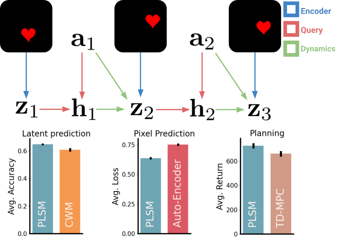
Figure 1: Overview: World models are commonly used to predict latent trajectories, predict sequences of pixel observations, and perform planning. We propose an architecture together with an information bottleneck for learning simple and parsimonious world models. Our method relies on a query network that extracts a sparse representation $\mathbf{h}_{t}$ for predicting latent transition dynamics. Combining our method with three different auxiliary loss functions for i) contrastive learning ii) pixel prediction and iii) planning, we see consistent performance improvement in all three domains. Bars show mean score statistics aggregated over evaluation environments and seeds. Error bars represent standard error of the mean.

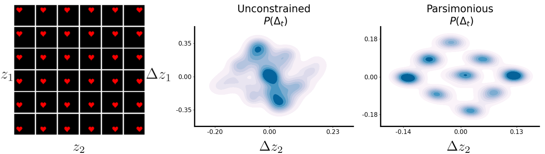
Figure 2: The heart (left) can appear on any $x,y$ coordinate in a two-dimensional latent space with boundaries, on which it can transition in 9 different ways (moving in eight directions and standing still, for instance when moving into a boundary). Encouraging dynamics to be parsimonious recovers these 9 different possible transitions (see right), whereas an unconstrained model (see center) does not.

To act adaptively in the high-dimensional dynamical system that is our world, humans build predictive models of their environment, capturing variation at various levels of complexity (Creutzig et al., 2009; Tishby & Polani, 2010). These world models allow us to forecast the future, imagine possibilities and counterfactuals, and plan to make desired outcomes more likely. Humans favor simple and parsimonious ways of describing and predicting the world (Chater & Vitányi, 2003; Rasmussen & Ghahramani, 2000). In the natural sciences, for example, we propose laws that allow us to predict events and natural phenomena not only accurately, but also succinctly. In a similar vein, compression lies at the heart of several modeling techniques in machine learning: World models (Ha & Schmidhuber, 2018; Kipf et al., 2019; Hafner et al., 2019a) represent the state of the world $\mathbf{s}_{t}$ at time $t$ and its dynamics in compact latent states $\mathbf{z}_{t}$. These latent state spaces abstract away from low-level details in $\mathbf{s}_{t}$, which makes it tractable to model how the environment changes over time $\Delta_{t}^{\mathbf{a}_{t}}=\mathbf{z}_{t+1}-\mathbf{z}_{t}$, given the agent’s actions $\mathbf{a}_{t}$. While latent state compression has been studied extensively (Ha & Schmidhuber, 2018; Micheli et al., 2022; Villegas et al., 2019; Watter et al., 2015), simple latent representations do not automatically give rise to simple latent dynamics of the sort humans create, say when formulating scientific theories: The inferred dynamics of the world model can still be very complex. By complex we mean that the precise nature of the dynamics $\Delta_{t}^{\mathbf{a}_{t}}$ varies substantially with the latent state variable $\mathbf{z}_{t}$, making the consequences of actions unpredictable without information about $\mathbf{z}_{t}$. In this paper, we therefore tackle the problem of learning world models whose latent dynamics are simple.

We introduce a regularization method that simplifies not only state representations but also the latent dynamics constructed by world models. Dynamics are simplified by minimizing the mutual information between two variables, the latent states $\mathbf{z}_{t}$ and the inferred dynamics $\Delta_{t}^{\mathbf{a}_{t}}$, conditioned on the agent’s actions $\mathbf{a}_{t}$.

Our regularization method is both general and simple: We combine it with three classes of world models (see Fig. 1), used for future latent state prediction (Kipf et al., 2019), future pixel prediction (Hafner et al., 2019b), and planning (Hansen et al., 2022; Tang et al., 2023). Across these three model classes, we show that our regularization scheme improves models’ latent prediction accuracy, reconstruction ability, generalization and robustness properties, and ability to solve high-dimensional continuous control problems.

2 Latent dynamics

We assume that sequences of states and actions (and possibly rewards) are observed in a Markov Decision Process (MDP). An MDP consists of a state space $\mathcal{S}$, an action space $\mathcal{A}$, and transition dynamics $\mathbf{s}_{t+1}\sim P(\mathbf{s}_{t+1}|\mathbf{s}_{t},\mathbf{a}_{t})$ determining how the state evolves with the actions the agent performs. In reinforcement learning (RL), we additionally care about the reward function $r(\mathbf{s}_{t},\mathbf{a}_{t})$, which maps state-action pairs to a scalar reward term. Here, the goal is to learn the optimal policy $\pi_{\theta}(\mathbf{a}_{t}|\mathbf{s}_{t})$ that maps states to the actions with the highest possible $Q$-values $Q_{\pi_{\theta}}(\mathbf{s}_{t},\mathbf{a}_{t})=\mathbb{E}_{\pi_{\theta}}\left[\sum_{t=1}^{T}\gamma^{t}r(\mathbf{s}_{t},\mathbf{a}_{t})\right]$, where $\gamma$ is a discount factor. In this paper, we consider latent dynamics learning both in reward-free and RL settings.

We consider world models that are trained to predict their future state representations. Instead of predicting the future in a potentially high-dimensional state-space, prediction happens in a compressed latent space: First, the current state $\mathbf{s}_{t}$ is transformed using an encoder into a latent state $\mathbf{z}_{t}$ that compactly represents the agent’s sensory observation (Eq. 1). Then, given the action, the world model predicts the change in its latent state, $\Delta_{t}^{\mathbf{a}_{t}}$ that is induced by action $\mathbf{a}_{t}$ (Eq. 2 & 3).

$$\mathbf{z}_{t}=e_{\theta}(\mathbf{s}_{t})$$ (1)

$$\Delta_{t}=d_{\theta}(\mathbf{z}_{t},\mathbf{a}_{t})$$ (2)

$$\tilde{\mathbf{z}}_{t+1}=\mathbf{z}_{t}+\Delta_{t}$$ (3)

We omit the action superscript from $\Delta_{t}$ for simplicity. Here, $e_{\theta}$ is the encoder network mapping states to latent states, and $d_{\theta}$ is the dynamics network mapping $\mathbf{z}_{t}$ and $\mathbf{a}_{t}$ to $\Delta_{t}$. Dynamics and latent representations are fully deterministic in our setup, but can easily be probabilistic by predicting the means and standard deviations of Gaussians.

2.1 Parsimonious latent dynamics

$\Delta_{t}$ captures the dynamics of the latent space that the world model has constructed. Consider the marginal probability distribution of state transitions $P(\Delta_{t}|\mathbf{a}_{t})$ given the agent’s actions. If an environment has simple transition dynamics, the entropy of $P(\Delta_{t}|\mathbf{a}_{t})$ will be low. More concretely, only a small set of different $\Delta_{t}$ will be necessary to describe how the states evolve, depending on the actions. The level of description is crucial here. An environment emitting pixel observations may not appear to have parsimonious dynamics when only considering transitions in pixel space. However, when represented in a compact latent space, $P(\Delta_{t}|\mathbf{a}_{t})$ may have much lower entropy. Moreover, since the latent space is constructed by the model’s encoder $e_{\theta}$, we can guide it to construct a latent space that is such that the entropy of $P(\Delta_{t}|\mathbf{a}_{t})$ is low.

To obtain a tractable way of minimizing the complexity of the latent dynamics while retaining an expressive world model, we propose to minimize the mutual information between the latent state $\mathbf{z}_{t}$ and the dynamics $\Delta_{t}$, conditioned on the agent’s action.

$$I(\mathbf{z}_{t};\Delta_{t}|\mathbf{a}_{t})=\mathcal{H}[\Delta_{t}|\mathbf{a}_{t}]-\mathcal{H}[\Delta_{t}|\mathbf{z}_{t},\mathbf{a}_{t}]$$ (4)

Here $\mathcal{H}[\cdot]$ denotes the Shannon entropy. The mutual information represents how many bits of information the latent state $\mathbf{z}_{t}$ carries about the latent dynamics $\Delta_{t}$, after conditioning on the action that was selected. If this quantity is 0, the latent dynamics $\Delta_{t}$ do not depend on $\mathbf{z}_{t}$ but vary only depending on the agent’s action $\mathbf{a}_{t}$. In this case, $e_{\theta}$ can be seen as an equivariant map between the states and latent states (Cohen & Welling, 2016; Shewmake et al., 2023). We propose to learn dynamics that are softly state-invariant, in that they depend only minimally on $\mathbf{z}_{t}$, and principally on $\mathbf{a}_{t}$. If the environment dynamics can indeed be expressed in simple terms on a particular level of description, having the inductive bias that the dynamics are simple can allow the model to discover this latent space more efficiently. Secondly, generalization about novel state transitions may be easier if the dynamics depend mostly on the action, and not the latent state.

3 Model

In this section, we introduce our Parsimonious Latent Space Model (PLSM). The PLSM learns an encoder and dynamics model $e_{\theta},d_{\theta}$ that captures environment dynamics as accurately as possible, while minimizing $I(\mathbf{z}_{t};\Delta_{t}|\mathbf{a}_{t})$. Since we are working in a latent space constructed by $e_{\theta}$, the mutual information term could be minimized by not giving the dynamics model any information about the latent state $\Delta_{t}=d_{\theta}(\mathbf{a}_{t})$. In this extreme, all $\Delta_{t}$ are predicted exclusively by the action. However, it is very rarely the case that the action can capture an environment’s full dynamics (see Fig. 2). In a grid world with walls, the action ’UP’ will move the agent along the grid’s y-axis, except when the agent is facing a wall. As such, a minimal amount of information about the state is necessary to successfully predict future latent states.

Instead, we propose to make the dynamics softly state-invariant: From $\mathbf{z}_{t}$ and $\mathbf{a}_{t}$, we infer a variable that contains the minimal amount of information needed to accurately predict the correct transition $\Delta_{t}$. We introduce a query network $f_{\theta}$ which maps latent state-action pairs to a latent code $\mathbf{h}_{t}$. We modify the next-step prediction components accordingly

$$\mathbf{h}_{t}=f_{\theta}(\mathbf{z}_{t},\mathbf{a}_{t})$$ (5)

$$\Delta_{t}=d_{\theta}(\mathbf{h}_{t},\mathbf{a}_{t})$$ (6)

We give the query network information about the action that the transition is conditioned on. This allows the network to attend to the relevant bits in $\mathbf{z}_{t}$ to output an appropriate $\mathbf{h}_{t}$. Finally, to make $\mathbf{h}_{t}$ represent only the minimal amount of information needed to predict the next state, provided that $\mathbf{a}_{t}$ is known, we penalize the norm of $\mathbf{h}_{t}$ (Ghosh et al., 2019; Yarats et al., 2021b). The strength of the penalization is controlled through a hyperparameter $\beta$. This regularization minimizes how much $\mathbf{h}_{t}$ can vary with $\mathbf{z}_{t}$ (up to noise) and hence their mutual information (see Appendix A). We then train our encoder $e_{\theta}$, query network $f_{\theta}$, and dynamics $d_{\theta}$ jointly to minimize the following information regularized loss function.

$$\mathcal{L}=||\mathbf{z}_{t}+d_{\theta}(\mathbf{h}_{t},\mathbf{a}_{t})-e_{\theta}(\mathbf{s}_{t+1})||_{2}^{2}+\beta||\mathbf{h}_{t}||_{2}^{2}$$ (7)

In contrast to information bottlenecks imposed on the latent states themselves, we apply an information bottleneck to the dynamics, making $\Delta_{t}$ easier to predict simply given $\mathbf{a}_{t}$. Notably, this can also lead to state compression, in that $e_{\theta}$ will be encouraged to omit features from $\mathbf{s}_{t+1}$ that cannot be predicted easily with little information from $\mathbf{z}_{t}$.

Unfortunately, the above loss function has a trivial solution: it can be minimized completely if $d_{\theta}$ and $e_{\theta}$ output a constant $\mathbf{0}$ vector for all states and state-action pairs (Tang et al., 2023). This issue is referred to as representational collapse. Representational collapse can be remedied in various ways. To show the generality of our information bottleneck, we combine it with three different auxiliary loss functions to avoid representational collapse and evaluate the resulting models on three different learning problems.

3.1 Representational collapse

Representational collapse can be avoided by encouraging the latent state to contain information about the original state. We present three popular methods for achieving this. In doing so, we recover three classes of sequential state-space models: Sequential Auto-Encoders (Kingma & Welling, 2013; Ghosh et al., 2019), Contrastive World Models (CWM) (Kipf et al., 2019), and Self Predictive Representation (SPR) models (Schwarzer et al., 2020; Tang et al., 2023). The PLSM can seamlessly be incorporated into any of these model classes. Across several experiments, we show that doing so increases i) models’ ability to accurately predict their encoding of future states, ii) their ability to accurately reconstruct future states from predicted latent, and iii) their viability as world models for use in planning and control.

Auto-Encoding models use a decoder network $g_{\theta}$ and train it, along with the encoder, to predict $\mathbf{s}_{t}$ from the encoded representation. Decoding the next state forces $\mathbf{z}_{t}$ to contain information about $\mathbf{s}_{t}$, preventing representational collapse. We make the Auto-Encoders sequential, training them to reconstruct the next state $\mathbf{s}_{t+1}$ from the predicted latent $\tilde{\mathbf{z}}_{t+1}=\mathbf{z}_{t}+\Delta_{t}$, and minimize the distance between predicted and encoded latents.

$$\mathcal{L}_{\text{AE}}=||\mathbf{z}_{t+1}-\tilde{\mathbf{z}}_{t+1}||_{2}^{2}+||\mathbf{s}_{t+1}-g_{\theta}(\tilde{\mathbf{z}}_{t+1})||_{2}^{2}\\$$ (8)

If the states are images, the last term in Eq. 8 can be replaced with a cross-entropy loss. An alternative to using a decoder is to augment the transition loss function with a contrastive objective. Contrastive objectives encourage that states are distinguishable in the latent space. That is, given a latent state and action, the model should maximize the distance between the correct future latent state $\mathbf{z}_{t+1}$, and other latent states in the training batch $\mathbf{z}^{-}$, up to a margin $\lambda$.

$$\mathcal{L}_{\text{C}}=||\mathbf{z}_{t+1}-\tilde{\mathbf{z}}_{t+1}||_{2}^{2}+\max(0,\lambda-||\mathbf{z}^{-}+\tilde{\mathbf{z}}_{t+1}||_{2}^{2})\\$$ (9)

The last class of models we consider, SPR models, avoids representational collapse by using a target encoder $e_{\theta}^{-}$ to obtain embeddings of the next state in Eq. 7. The stop-gradient operator $\mathrm{sg}(\cdot)$ is applied to the target representation, preventing $e_{\theta}^{-}$ from updating based on prediction errors. Instead, the target encoder weights are updated as an exponential moving average of the primary encoder’s weights at every other gradient step (Schwarzer et al., 2020). Even though this objective is minimized by trivial representations (e.g. $e_{\theta}(\mathbf{s}_{t})=e_{\theta}^{-}(\mathbf{s}_{t})=\mathbf{0}$), updating the target encoder with slower, semi-gradient methods prevents collapse in practice (Tang et al., 2023).

$$\mathcal{L}_{\text{SPR}}=||\mathbf{z}_{t}+d_{\theta}(\mathbf{z}_{t},\mathbf{a}_{t})-\mathrm{sg}(e_{\theta}^{-}(\mathbf{s}_{t+1}))||_{2}^{2}$$ (10)

SPR models have become prevalent in RL, where their ability to compress away information in the state that is irrelevant for value and policy learning makes them useful for representation learning and planning (Schwarzer et al., 2020; Hansen et al., 2022). In the following experiments, we evaluate the effect of applying our regularization to these different dynamics models.

4 Related work

Our approach introduces a mutual information constraint between the latent states $\mathbf{z}_{t}$ and the latent dynamics $\Delta_{t}$ inferred by the model. Several methods focus on state compression for dynamics modeling (Ha & Schmidhuber, 2018; Hafner et al., 2019b; Schwarzer et al., 2020; Hansen et al., 2022; Higgins et al., 2017): The Recurrent State Space Model (RSSM) (Hafner et al., 2019b, a, 2020), uses a variational Auto-Encoder in combination with a recurrent model (e.g. a GRU (Chung et al., 2014)) to infer compact latent states in partially observable environments. Latent consistency is enforced by minimizing the Kullback-Leibler (KL) divergence between latent states predicted by the model and latent states inferred from pixels. The KL term regularizes the latent not to contain more information than can be predicted by the dynamics model (Hafner et al., 2019a; Kingma & Welling, 2013). Unlike our approach, this information bottleneck is not applied to the dynamics $\Delta_{t}$ themselves, but to the representations $\mathbf{z}_{t}$. While simplified latents can make transition dynamics more tractable to model, they do not necessarily give rise to the simple, compressible dynamics that we are interested in.

Mutual information minimization is used in many deep learning frameworks more generally: Alemi et al. (2016) and Poole et al. (2019) use variational methods for minimizing the mutual information between the network’s inputs $X$ and latent representations $Z$ while maximizing the mutual information between representations $Z$ and outputs $Y$. Mutual information minimization also has links to generalization ability (Bassily et al., 2018; Achille & Soatto, 2018; Alemi, 2020), robustness in RL (Saanum et al., 2023; Eysenbach et al., 2021) and disentanglement (Higgins et al., 2016; Quessard et al., 2020).

Closest to our regularization method is the past-future information bottleneck (Creutzig et al., 2009; Bialek et al., 2001). Here the mutual information between sequences of past states and future states is minimized (Tishby & Polani, 2010; Amir et al., 2015). While this method simplifies dynamics, our approach differs in important ways: Rather than representing the environment’s dynamics, say, using a low number of its principal components (e.g. slow feature analysis), we treat the dynamics operator $\Delta_{t}$ itself as a random variable, and minimize its conditional dependence on $\mathbf{z}_{t}$. Furthermore, when $\Delta_{t}$ is fully disentangled from $\mathbf{z}_{t}$, each action can be seen as a transformation that acts on the latent state space in the same way, invariantly of $\mathbf{z}_{t}$ (Kondor, 2008; Quessard et al., 2020). We model the dynamics as softly state-invariant, allowing us to predict future latents both accurately and parsimoniously.

Lastly, striving for simplicity is a defining trait of human cognition (Chater & Vitányi, 2003; Solomonoff, 1964): We prefer simple explanations of data (Rasmussen & Ghahramani, 2000; Bramley et al., 2017), assume that entities and events are related to each other in simple ways (Garvert et al., 2023; Demircan et al., 2023), and solve tasks and control problems using simple sequential strategies (Saanum et al., 2023; Gigerenzer & Gaissmaier, 2011; Lai & Gershman, 2021).

5 Experiments

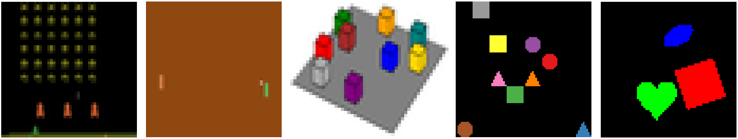
Figure 3: The five environments used to evaluate the accuracy of the latent dynamics. From left to right: Space Invaders, Pong, Cubes 9, Shapes 9, and dSprites.

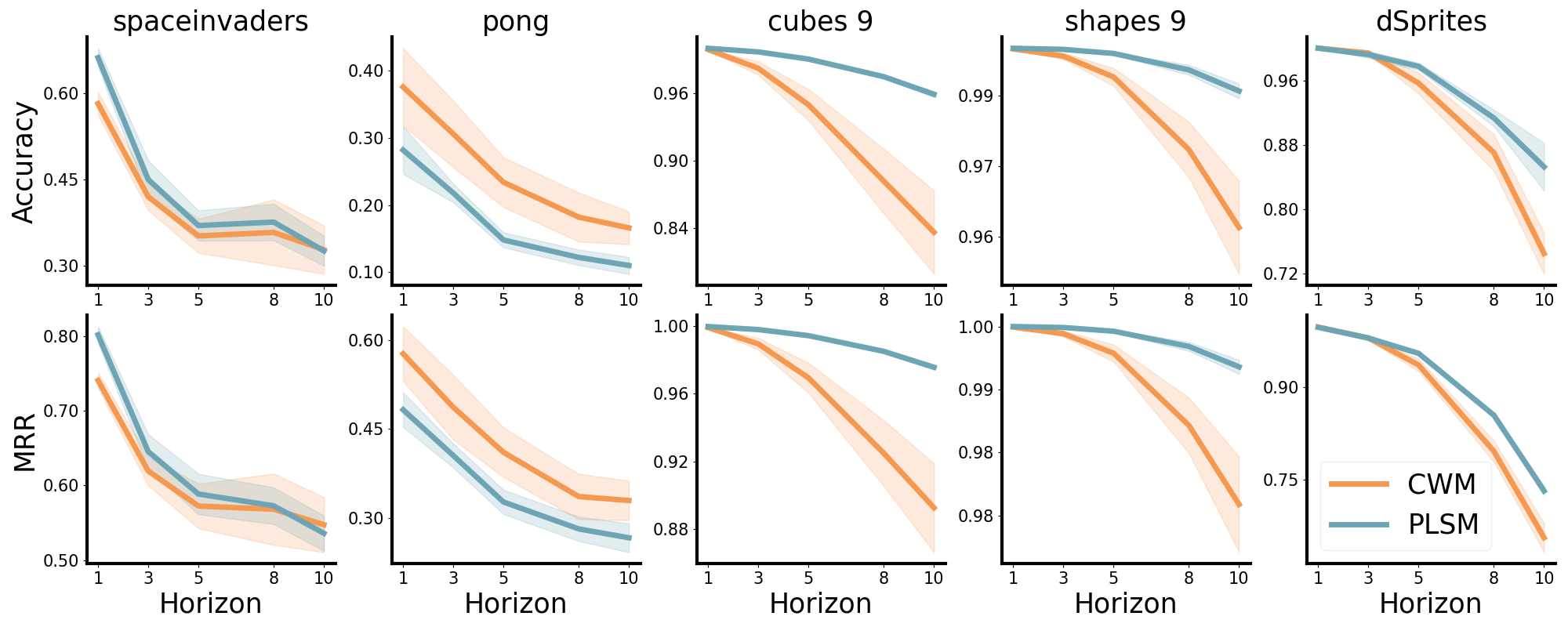
Figure 4: PLSM improves contrastive world models’ accuracy in long-horizon latent prediction in four out of five environments. In the cubes and shapes dataset, the PLSM is close to perfect even when predicting as far as 10 timesteps in the future. Lines show accuracy on entire test data averaged over five random seeds. The shaded region corresponds to the standard error of the mean.

We validated whether PLSM, when incorporated in the three model classes discussed in Section 3.1, can learn accurate latent transition models in complex, pixel-based environments. Using the evaluation framework and environments from Kipf et al. (2019) (see Fig. 3 for example observations), we generated datasets of image, action, next-image triplets from two Atari games (Pong and Space Invaders), and grid worlds with moving 3D cubes and 2D shapes, where each action corresponds to moving an object in one of four cardinal directions. Importantly, these objects are not allowed to occupy the same position on the grid. The models therefore have to use information about objects’ relative positions to predict if they will move in a particular direction or collide. To make the learning tasks more challenging, we increased the number of movable cubes and shapes from 5 to 9, producing 36-dimensional one-hot encoded action space $|\mathcal{A}|=4\times 9$. We also increased the size of the grid they could move on from $5\times 5$ to $8\times 8$, and reduced the amount of training data by 1/4th. We refer to these environments as cubes 9 and shapes 9, respectively.

We also created an environment based on the dSprite dataset (Matthey et al., 2017), with three sprites traversing latent generative factors on a random walk. The sprites had 6 generative factors: Spatial $x,y$ coordinates, scale, rotation, color, and shape. The sprites could vary in coordinates, scale, and rotation within episodes, and additionally vary in color across episodes. Using again a one-hot encoded action space per generative feature, we end up with an action space size of $|\mathcal{A}|=3\times 8$.

5.1 Future state prediction

We evaluated our reconstruction-based and contrastive models in their ability to capture the latent dynamics in the environments introduced above accurately. Due to the models being trained with different loss functions, we evaluated them using separate methods: Contrastive models were scored based on their ability to correctly distinguish between distinct future states (e.g. latent prediction accuracy), whereas Auto-Encoding models were scored according to their ability to predict pixels. Contrastive models were trained for 100 epochs except for in the Atari environments where they were trained for 200 epochs, like in Kipf et al. (2019). Reconstruction-based models were always trained for 200 epochs. We evaluated the contrastive models using the same metrics and methods used in Kipf et al. (2019): Given a state $\mathbf{s}_{t}$, a sequence of $N$ actions $\mathbf{a}_{t},...,\mathbf{a}_{t+N-1}$, and the resulting state $\mathbf{s}_{t+N}$, we make the model predict its latent representation of $\mathbf{s}_{t+N}$ from the initial state and action sequence. The models were evaluated at several prediction horizons. Finally, we report the Hits at Rank 1 accuracy and Mean Reciprocal Rank for left-out transition, which reflect the Euclidean distance between the predicted latent and the encoding of $\mathbf{s}_{t+N}$, relative to the other encoded states in the test set. Similarly, the Auto-Encoding models were evaluated based on how well they predicted future pixel observations in the test dataset, across several horizons. Here we report the mean pixel-wise cross-entropy error.

5.2 Baselines

As a baseline for the PLSM with the contrastive objective, we used the unregularized contrastive model from Kipf et al. (2019) without slots or a Graph Neural Network (GNN (Schlichtkrull et al., 2018; Kipf & Welling, 2016)). We refer to this model as CWM (for Contrastive World Model), and its dynamics are defined through Equation 1 - 3 and 9. The slot-based version of this model, C-SWM, performed close to perfectly on the original, easier cubes and shapes datasets. We also evaluate C-SWM on our more challenging version of the cubes dataset both with and without mutual information regularization (see Appendix D for results). For reconstruction, we used a sequential Auto-Encoder, whose dynamics are defined by Equation 1 - 3 and 8.

6 Results

We trained contrastive models both with and without our regularization. We fitted the regularization coefficient $\beta$ with a grid search and found a value of $0.1$ to work the best. PLSM could better predict its own representations further into the future in four of the five tasks (Fig. 4). We see the greatest gains in the cubes and shapes environments. Here, all 9 objects can interact with each other and the grid boundaries depending on their position. Always considering all possible interactions makes it challenging for a model to generalize to novel transitions. A more parsimonious solution is simply to represent whether or not the object in question would collide or not if moved in the direction specified by $\mathbf{a}_{t}$. Our results suggest that our regularization can help learn such representations, affording better generalization to left-out transitions.

The performance of the slotted model, C-SWM, decreased slightly in the more challenging cubes 9 dataset. However, applying our mutual information regularizer to its dynamics improved the accuracy back to near perfection, suggesting that the regularization can be beneficial for slotted models in complex multi-object environments. See Appendix D for details.

In one environment, Pong, we do not see an advantage in encouraging parsimonious dynamics. Here, various components are outside of the agent’s sphere of influence, for instance, the movement of the opponent’s paddle. This makes it challenging for the PLSM to capture all aspects of the environment state in its dynamics. In environments with non-controllable dynamics, we offer a remedy by only enforcing half of the latent space to be governed by parsimonious dynamics, and allowing the other half to be unconstrained. This hybrid model in turn shows the strongest performance in the Atari environments. See Appendix C for details.

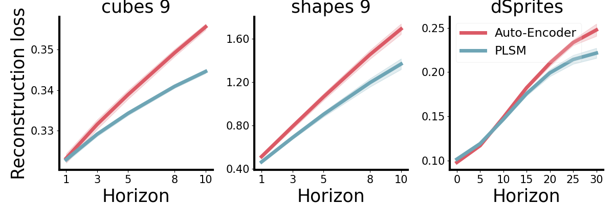
Figure 5: Regularization had a similar positive effect on Auto-Encoding models. Over longer horizons, pixel reconstruction was more accurate with mutual information-constrained dynamics. Lines show accuracy on entire test data averaged over five random seeds. The shaded region corresponds to the standard error of the mean.

For Auto-Encoding models we again fitted the regularization scale hyperparameter $\beta$ and found a value of $1$ to work the best. We saw similar accuracy gains for the Auto-Encoding models (Fig. 5): Regularizing the dynamics allowed for more accurate long-horizon pixel prediction in the cubes, shapes, and dSprite environment. In the dSprite environment, we evaluated the reconstruction-based models on longer prediction horizons to bring out differences in the models’ ability to predict environment dynamics accurately.

7 Generalization and robustness

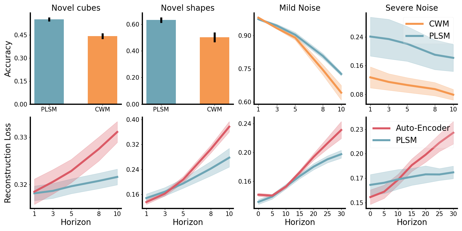
Figure 6: PLSM improves generalization and robustness of both contrastive (top) and Auto-Encoding models (bottom): When exposed to scenes with fewer objects than trained on, or corrupted data from the test set, PLSM improves both accuracy over the CWM and future pixel prediction ability over the Auto-Encoder. Lines represent the average of models trained across five seeds. Shaded regions and bars reflect the standard error of the mean.

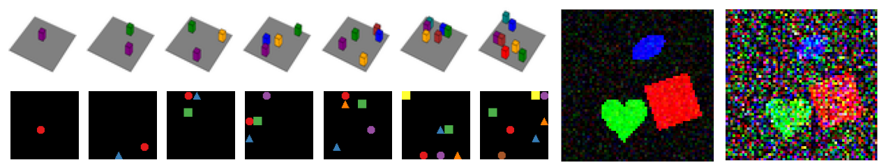
Figure 8: Datasets used to probe generalization and robustness. Left: Cubes and shapes data with varying numbers of objects. Right: dSprite images with mild and severe noise corruption.

Next, we evaluated the generalization and robustness properties of PLSM. For the cubes and shapes environments, we generated novel datasets where the number of moving objects was lower than in the original training data. In these datasets, the number of moving objects varied from 1 to 7. We also probed the models’ robustness to noise. We corrupted test data from the dSprite environment with noise sampled from Gaussian distributions. Models were tested both in a mild noise ($\sigma=0.1$) and a severe noise ($\sigma=0.5$) condition. See Supplementary Fig. 8 for example data.

We used the same evaluation methods for both contrastive and Auto-Encoding models to probe generalization and robustness properties. When tested on scenes with fewer objects than the training data, we see a general decrease in accuracy among contrastive models because of the domain shift. Still, with our information-theoretic dynamics bottleneck the model generalizes significantly better to the out-of-distribution transition data (Fig. 6). Since PLSM seeks to predict the next state using as little information from its latent representations as possible, it is more likely to learn that the blocks move in a way that is generally invariant to the number of other blocks in the scene. In the same vein, PLSM also allows for more accurate reconstruction of future pixel observations in the novel cube and shape environments.

Lastly, corrupting the observations with Gaussian noise had a stronger negative effect on the unconstrained dynamics models than on the PLSM: In the severe noise condition, the PLSM dynamics still accurately predict 1/5th of the transitions after 10 steps, whereas the unconstrained dynamics, more susceptible to rely on noisy information in the state, only predict 1/10th accurately.

In sum, parsimonious dynamics regularization improves both generalization and robustness properties in the three environments. The mutual information bottleneck on $\Delta_{t}$ therefore not only improves prediction accuracy for data in the training distribution, but may also allow the model to generalize better to out-of-distribution data, and improve its robustness to noisy observations.

8 Parsimonious dynamics for control

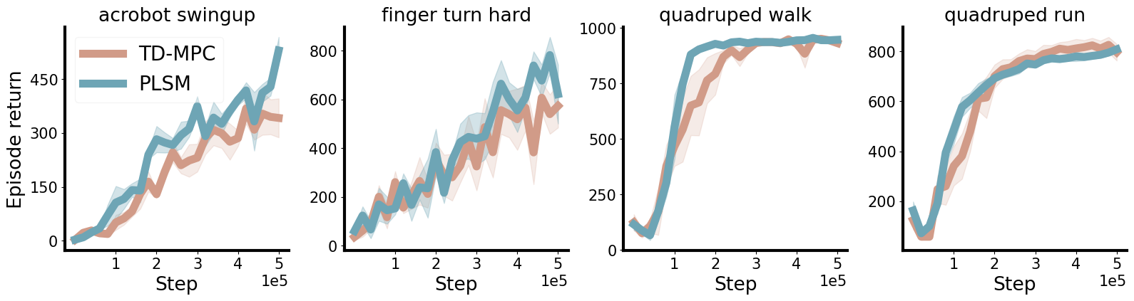
Figure 7: PLSM, when incorporated into the TD-MPC algorithm, improves planning in continuous control tasks with high-dimensional and complex dynamics, improving sample efficiency in Quadruped Walk and final performance in Acrobot Swingup and Finger Turn Hard. Lines show the average return attained across 15 evaluation episodes, averaged over five seeds. The shaded region represents the standard error of the mean over the five seeds.

Finally, we evaluated the PLSM’s effect on planning algorithms’ ability to learn policies in continuous control tasks. To do so, we built upon the TD-MPC algorithm (Hansen et al., 2022), an algorithm that jointly learns a latent dynamics model and performs policy search by planning in the model’s latent space.

TD-MPC makes use of a Task-Oriented Latent Dynamics (TOLD) model. This dynamics model is trained to predict its own future state representations from an initial state and action sequence while making sure that the controller’s policy $\pi_{\theta}$ and $Q$-value function are decodable from the latent state (hence the name task-oriented latent dynamics). Importantly, TOLD falls under the category of SPR models, since it uses an exponentially moving target encoder $e_{\theta}^{-}$ with the stop-gradient operator to learn to predict its own representations. For planning TD-MPC uses the Cross-Entropy Method (Rubinstein, 1999), searching for actions that maximize $Q$-values.

Only minimal adjustments to the TOLD model are necessary to attain parsimonious dynamics. Instead of predicting the next latent directly from the current latent and action $\tilde{\mathbf{z}}_{t+1}=d_{\theta}(\mathbf{z}_{t},\mathbf{a}_{t})$, we use a query network $f_{\theta}$, mapping latent state-action tuples to $\mathbf{h}_{t}$ and then minimize

$$\mathcal{L}=||\mathbf{z}_{t}+d_{\theta}(\mathbf{h}_{t},\mathbf{a}_{t})-\mathrm{sg}(e_{\theta}^{-}(\mathbf{s}_{t+1}))||_{2}^{2}$$

We evaluated the efficacy of parsimonious dynamics for control in four state-based continuous control tasks from the DeepMind Control Suite (Tassa et al., 2018). We chose the following environments: i) Acrobot Swingup, due to its challenging and chaotic dynamics. ii) Finger Turn Hard, which poses a challenging exploration problem that TD-MPC was found to struggle with. iii) Quadruped Walk and iv) Quadruped Run due to the high-dimensional dynamics. These tasks have dynamics that appear complex in the original state-space but could potentially be simplified in an appropriate latent space by introducing a dynamics bottleneck.

We trained the latent dynamics and planning models in the four tasks across 500k environment steps. Scores for TD-MPC are obtained from the original implementation provided by the authors. We again used $\beta=0.1$ for all tasks. We see clear performance gains due to the parsimonious dynamics in the Acrobot Swingup, Finger Turn Hard, and Quadruped Walk environments, with more subtle benefits in Quadruped Run (Fig. 7). In the Acrobot and Finger environments, the simplified dynamics led to significantly higher scores. In the Quadruped tasks, while the asymptotic performance is comparable, planning with parsimonious dynamics led to faster learning. In fact, in Quadruped Walk, PLSM achieves asymptotic performance roughly 100k environment steps before the original TD-MPC. In sum, our results suggest that modeling the world with simple dynamics could be beneficial for RL and trajectory optimization.

9 Conclusion

We have proposed a latent dynamics model that predicts future states while minimizing the dependence between the predicted dynamics $\Delta_{t}$ and the latent state representations $\mathbf{z}_{t}$. Optimizing this objective effectively simplifies the latent dynamics, lowering the conditional entropy of the dynamics given the actions $\mathcal{H}[\Delta_{t}|\mathbf{a}_{t}]$, and making the effect of the actions on the agent’s latent state more predictable.

Combining our objective with three different model classes – contrastive world models, sequential Auto-Encoders, and SPR models – we observed consistent improvements in models’ ability to accurately predict their own representations, predict future pixel observations, generalize to novel and noisy environments, and perform planning in high-dimensional environments with complex dynamics.

A promising future direction is to combine our mutual information regularization with recurrent models. In partially observable, non-Markovian environments, next-state prediction is often done with a recurrent model that uses the agent’s history as input. Using our bottleneck here would correspond to the assumption that, although the dynamics often depend in subtle ways on the agent’s history, we do not need to pay attention to all bits from the distant past to predict the impact of our actions on our state. Such a model would represent the dynamics as softly non-Markovian and could lead to stronger generalization for prediction and control. Future work could also investigate how our regularization impacts the structure of the latent state representations inferred by the model.

Lastly, we saw a positive effect of applying our regularization to the slot-based world model from Kipf et al. (2019). In the cubes and shapes environments, objects interact with each other in simple ways. However, the more objects there are the more possible interactions between them. Learning which interactions to pay attention to, for instance with our mutual information regularization, could be a promising avenue for object-centric learning (Johnson et al., 2017; Locatello et al., 2020; Buschoff et al., 2023).

Overall, our results suggest that the inductive bias that the world can be predicted with simple rules and laws offers consistent improvements in world models’ accuracy, generalization ability, and robustness.

Impact Statement

We present a method for regularizing world models. Our results suggest that simplifying world model dynamics can improve their accuracy and performance in downstream tasks. Improving the representational and predictive abilities of world models can have societal consequences, none of which we feel must be specifically discussed here.

Appendix A Mutual Information minimization

To simplify dynamics, our algorithm minimizes the mutual information between $\mathbf{z}_{t}$ and $\Delta_{t}$ conditioned on $\mathbf{a}_{t}$ (Eq. 7 & 2). With stochastic gradient descent, we search for parameters $\theta$ that optimize the following objective:

$$\min_{\theta}I(\mathbf{z}_{t};\Delta_{t}|\mathbf{a}_{t})$$ (11)

To do so, we introduce a new variable $\mathbf{h}_{t}$ that depends on $\mathbf{z}_{t}$ and $\mathbf{a}_{t}$ (Eq. 5). We use this variable, together with $\mathbf{a}_{t}$, to produce $\Delta_{t}$, instead of $\mathbf{z}_{t}$. For a specific $\mathbf{a}_{t}$, the Markov chain behind $\Delta_{t}^{\mathbf{a}_{t}}$ can be written as

$$\mathbf{z}_{t}\rightarrow\mathbf{h}_{t}\rightarrow\Delta_{t}^{\mathbf{a}_{t}}$$ (12)

Thus, to minimize the mutual information between $\mathbf{z}_{t}$ and $\Delta_{t}$, we can instead minimize the mutual information between $\mathbf{z}_{t}$ and $\mathbf{h}_{t}$: $\min_{\theta}I(\mathbf{z}_{t};\mathbf{h}_{t}|\mathbf{a}_{t})$. Following Alemi et al. (2016), we write the mutual information between $\mathbf{z}_{t}$ and $\mathbf{h}_{t}$ as follows:

$$I(\mathbf{z}_{t};\mathbf{h}_{t}|\mathbf{a}_{t})=\int d\mathbf{z}\>d\mathbf{h}\>d\mathbf{a}\>p(\mathbf{z},\mathbf{h},\mathbf{a})\log\dfrac{p(\mathbf{h}|\mathbf{z},\mathbf{a})}{p(\mathbf{h}|\mathbf{a})}$$ (13)

In our case, $p(\mathbf{h}|\mathbf{z},\mathbf{a})$ is deterministic. The marginal distribution conditioned on $\mathbf{a}$, $p(\mathbf{h}|\mathbf{a})$, is challenging to obtain. We instead use a variational approximation: With our variational distribution $q(\mathbf{h}|\mathbf{a})$, we can upper bound the mutual information as follows

$$I(\mathbf{z}_{t};\mathbf{h}_{t}|\mathbf{a}_{t})=\int d\mathbf{z}\>d\mathbf{h}\>d\mathbf{a}\>p(\mathbf{z},\mathbf{a})p(\mathbf{h}|\mathbf{z},\mathbf{a})\log\dfrac{p(\mathbf{h}|\mathbf{z},\mathbf{a})}{q(\mathbf{h}|\mathbf{a})}$$ (14)

First, this upper bound lets us see that the mutual information can be minimized by minimizing the number of bits of information $\mathbf{z}_{t}$ contains about $\mathbf{h}_{t}$ over and above $\mathbf{a}_{t}$. This could potentially be done by introducing a parameterized prior that depends on $\mathbf{a}_{t}$, $q_{\theta}(\mathbf{h}_{t}|\mathbf{a}_{t})$ and minimize the KL divergence between these two probability distributions

$$KL_{D}[p(\mathbf{h}_{t}|\mathbf{z}_{t},\mathbf{a}_{t})||q_{\theta}(\mathbf{h}_{t}|\mathbf{a}_{t})]$$ (15)

We opt for a simpler approach, that allows us to do this without introducing a new prior and parameterization. Following Ghosh et al. (2019), we assume that $q(\mathbf{h}_{t}|\mathbf{a}_{t})$ is a standard, $d$-dimensional, isotropic Gaussian distribution $\mathcal{N}(\mathbf{0},\mathbb{I})$. Assuming further that $\mathbf{h}_{t}$ is another $d$-dimensional isotropic Gaussian, the KL divergence is a function of the mean and standard deviation of $\mathbf{h}_{t}$ (Ghosh et al., 2019; Kingma & Welling, 2013):

$$2KL_{D}=||\mu(\mathbf{h}_{t})||_{2}^{2}+d+\sum_{i}^{d}\sigma(\mathbf{h}_{t})_{i}-\log\sigma(\mathbf{h}_{t})_{i}$$ (16)

Here $\mu(\cdot)$ and $\sigma(\cdot)$ return the mean and standard deviation of the Gaussian, respectively. Importantly, we can minimize the KL divergence by minimizing the first term in the above equation, which is simply the norm of the mean of $\mathbf{h}_{t}$. In our deterministic setup, we therefore simply minimize the norm of $\mathbf{h}_{t}$ itself.

Appendix B Generalization datasets

Appendix C Hybrid model

We propose a hybrid model for the Atari environments. The hybrid model splits the latent state in two, one parsimonious state space $\mathbf{z}_{t}^{1}$ and an unconstrained state space $\mathbf{z}_{t}^{2}$. To predict the next state, the model uses two dynamics MLPs $\tilde{\mathbf{z}}_{t+1}^{2}=\mathbf{z}_{t}^{2}+d_{\theta}^{1}(\mathbf{z}_{t}^{1},\mathbf{z}_{t}^{2},\mathbf{a}_{t})$ and $\tilde{\mathbf{z}}_{t+1}^{1}=\mathbf{z}_{t}^{1}+d_{\theta}^{2}(\mathbf{h}_{t},\mathbf{a}_{t})$. The next latent prediction is then defined as $\tilde{\mathbf{z}}_{t+1}=Concatenate(\tilde{\mathbf{z}}_{t+1}^{1},\tilde{\mathbf{z}}_{t+1}^{2})$. Results are shown in Fig. 9.

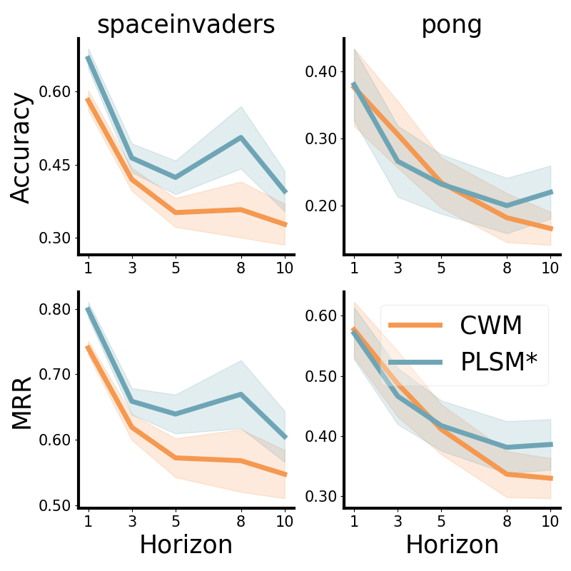
Figure 9: Our hybrid model, which splits the latent space into a parsimonious one and an unconstrained one, outperforms the baseline on long-horizon latent prediction in the Atari environments.

Appendix D Slots with information regularization

We evaluated the C-SWM on our cubes 9 task, both with and without our regularization. The performance of C-SWM dropper by a small amount due to the increased difficulty of the task for longer prediction horizons ($t=10$). Interestingly, using our regularization method proved beneficial for the slotted model, outperforming the unregularized C-SWM in long horizon latent prediction.

Table 1: PLSM with slots outperforms the C-SWM (Kipf et al., 2019) in latent prediction at prediction horizon $t=10$, averaged over five seeds, plus and minus standard error of the mean.

Accuracy	PLSM	C-SWM
Cubes 9	99.05% $\pm$0.18	97.45%$\pm$1.3

Appendix E Hyperparameters

E.1 Convolutional neural network architecture

To learn pixel representations we use a Convolutional Neural Network (CNN) architecture similar to the one used in Yarats et al. (2021b) and Yarats et al. (2021a). Auto-encoding models use an inverted version of this architecture for pixel reconstruction.

⬇

import torch

from torch import nn

encoder = nn.Sequential(

nn.Conv2d(num_channels, 32, 3, stride=2),

nn.ReLU(),

nn.Conv2d(32, 32, 3, stride=1),

nn.ReLU(),

nn.Conv2d(32, 32, 3, stride=1),

nn.ReLU(),

nn.Conv2d(32, 32, 3, stride=1),

nn.ReLU()

)

decoder = nn.Sequential(

nn.ConvTranspose2d(32, 32, 3, stride=1),

nn.ReLU(),

nn.ConvTranspose2d(32, 32, 3, stride=1),

nn.ReLU(),

nn.ConvTranspose2d(32, 32, 3, stride=1),

nn.ReLU(),

nn.ConvTranspose2d(32, num_channels, 4, stride=2),

nn.Sigmoid()

)

E.2 Contrastive models

Table 2: Contrastive model hyperparameters.

Hyperparameter	Value
Hidden units	512
Batch size	512
MLP hidden layers	2
Latent dimensions $|\mathbf{z}_{t}|$	50
Query dimensions $|\mathbf{h}_{t}|$	50
Regularization coefficient $\beta$	0.1
Margin $\lambda$	1
Learning rate	0.001
Activation function	ReLU (Nair & Hinton, 2010)
Optimizer	Adam (Kingma & Ba, 2014)

E.3 Reconstruction-based models

Table 3: Auto-Encoding model hyperparameters.

Hyperparameter	Value
Hidden units	512
Batch size	512
MLP hidden layers	2
Latent dimensions $|\mathbf{z}_{t}|$	50
Query dimensions $|\mathbf{h}_{t}|$	50
Regularization coefficient $\beta$	1.0
Learning rate	0.001
Activation function	ReLU (Nair & Hinton, 2010)
Optimizer	Adam (Kingma & Ba, 2014)
Reconstruction loss	Cross-entropy loss

E.4 DeepMind Control Suite

We use the same hyperparameters as Hansen et al. (2022) for the planning agents. The only addition is our PLSM regularization. We use a regularization coefficient of $0.1$ for all agents, and make the query net MLP $f_{\theta}$ the same size as the dynamics network $\mathbf{h}_{t}$, with $|\mathbf{h}_{t}|=|\mathbf{z}_{t}|$.

Table 4: Action repeat values in the DeepMind Control Suite tasks.

Task	Action repeat
Acrobot Swingup	4
Finger Turn Hard	2
Quadruped Walk	4
Quadruped Run	4

References

- Achille & Soatto (2018) Achille, A. and Soatto, S. Emergence of invariance and disentanglement in deep representations. The Journal of Machine Learning Research, 19(1):1947–1980, 2018.
- Alemi (2020) Alemi, A. A. Variational predictive information bottleneck. In Symposium on Advances in Approximate Bayesian Inference, pp. 1–6. PMLR, 2020.
- Alemi et al. (2016) Alemi, A. A., Fischer, I., Dillon, J. V., and Murphy, K. Deep variational information bottleneck. arXiv preprint arXiv:1612.00410, 2016.
- Amir et al. (2015) Amir, N., Tiomkin, S., and Tishby, N. Past-future information bottleneck for linear feedback systems. In 2015 54th IEEE Conference on Decision and Control (CDC), pp. 5737–5742. IEEE, 2015.
- Bassily et al. (2018) Bassily, R., Moran, S., Nachum, I., Shafer, J., and Yehudayoff, A. Learners that use little information. In Algorithmic Learning Theory, pp. 25–55. PMLR, 2018.
- Bialek et al. (2001) Bialek, W., Nemenman, I., and Tishby, N. Predictability, complexity, and learning. Neural computation, 13(11):2409–2463, 2001.
- Bramley et al. (2017) Bramley, N. R., Dayan, P., Griffiths, T. L., and Lagnado, D. A. Formalizing neurath’s ship: Approximate algorithms for online causal learning. Psychological review, 124(3):301, 2017.
- Buschoff et al. (2023) Buschoff, L. M. S., Schulz, E., and Binz, M. The acquisition of physical knowledge in generative neural networks. In International Conference on Machine Learning, pp. 30321–30341. PMLR, 2023.
- Chater & Vitányi (2003) Chater, N. and Vitányi, P. Simplicity: a unifying principle in cognitive science? Trends in cognitive sciences, 7(1):19–22, 2003.
- Chung et al. (2014) Chung, J., Gulcehre, C., Cho, K., and Bengio, Y. Empirical evaluation of gated recurrent neural networks on sequence modeling. arXiv preprint arXiv:1412.3555, 2014.
- Cohen & Welling (2016) Cohen, T. and Welling, M. Group equivariant convolutional networks. In International conference on machine learning, pp. 2990–2999. PMLR, 2016.
- Creutzig et al. (2009) Creutzig, F., Globerson, A., and Tishby, N. Past-future information bottleneck in dynamical systems. Physical Review E, 79(4):041925, 2009.
- Demircan et al. (2023) Demircan, C., Saanum, T., Pettini, L., Binz, M., Baczkowski, B. M., Kaanders, P., Doeller, C. F., Garvert, M. M., and Schulz, E. Language aligned visual representations predict human behavior in naturalistic learning tasks. arXiv preprint arXiv:2306.09377, 2023.
- Eysenbach et al. (2021) Eysenbach, B., Salakhutdinov, R. R., and Levine, S. Robust predictable control. Advances in Neural Information Processing Systems, 34:27813–27825, 2021.
- Garvert et al. (2023) Garvert, M. M., Saanum, T., Schulz, E., Schuck, N. W., and Doeller, C. F. Hippocampal spatio-predictive cognitive maps adaptively guide reward generalization. Nature Neuroscience, 26(4):615–626, 2023.
- Ghosh et al. (2019) Ghosh, P., Sajjadi, M. S., Vergari, A., Black, M., and Schölkopf, B. From variational to deterministic autoencoders. arXiv preprint arXiv:1903.12436, 2019.
- Gigerenzer & Gaissmaier (2011) Gigerenzer, G. and Gaissmaier, W. Heuristic decision making. Annual review of psychology, 62:451–482, 2011.
- Ha & Schmidhuber (2018) Ha, D. and Schmidhuber, J. Recurrent world models facilitate policy evolution. Advances in neural information processing systems, 31, 2018.
- Hafner et al. (2019a) Hafner, D., Lillicrap, T., Ba, J., and Norouzi, M. Dream to control: Learning behaviors by latent imagination. arXiv preprint arXiv:1912.01603, 2019a.
- Hafner et al. (2019b) Hafner, D., Lillicrap, T., Fischer, I., Villegas, R., Ha, D., Lee, H., and Davidson, J. Learning latent dynamics for planning from pixels. In International Conference on Machine Learning, pp. 2555–2565. PMLR, 2019b.
- Hafner et al. (2020) Hafner, D., Lillicrap, T., Norouzi, M., and Ba, J. Mastering atari with discrete world models. arXiv preprint arXiv:2010.02193, 2020.
- Hansen et al. (2022) Hansen, N., Wang, X., and Su, H. Temporal difference learning for model predictive control. arXiv preprint arXiv:2203.04955, 2022.
- Higgins et al. (2016) Higgins, I., Matthey, L., Pal, A., Burgess, C., Glorot, X., Botvinick, M., Mohamed, S., and Lerchner, A. beta-vae: Learning basic visual concepts with a constrained variational framework. Open Review, 2016.
- Higgins et al. (2017) Higgins, I., Pal, A., Rusu, A., Matthey, L., Burgess, C., Pritzel, A., Botvinick, M., Blundell, C., and Lerchner, A. Darla: Improving zero-shot transfer in reinforcement learning. In International Conference on Machine Learning, pp. 1480–1490. PMLR, 2017.
- Johnson et al. (2017) Johnson, J., Hariharan, B., Van Der Maaten, L., Fei-Fei, L., Lawrence Zitnick, C., and Girshick, R. Clevr: A diagnostic dataset for compositional language and elementary visual reasoning. In Proceedings of the IEEE conference on computer vision and pattern recognition, pp. 2901–2910, 2017.
- Kingma & Ba (2014) Kingma, D. P. and Ba, J. Adam: A method for stochastic optimization. arXiv preprint arXiv:1412.6980, 2014.
- Kingma & Welling (2013) Kingma, D. P. and Welling, M. Auto-encoding variational bayes. arXiv preprint arXiv:1312.6114, 2013.
- Kipf et al. (2019) Kipf, T., Van der Pol, E., and Welling, M. Contrastive learning of structured world models. arXiv preprint arXiv:1911.12247, 2019.
- Kipf & Welling (2016) Kipf, T. N. and Welling, M. Variational graph auto-encoders. arXiv preprint arXiv:1611.07308, 2016.
- Kondor (2008) Kondor, I. R. Group theoretical methods in machine learning. Columbia University, 2008.
- Lai & Gershman (2021) Lai, L. and Gershman, S. J. Policy compression: An information bottleneck in action selection. In Psychology of Learning and Motivation, volume 74, pp. 195–232. Elsevier, 2021.
- Locatello et al. (2020) Locatello, F., Weissenborn, D., Unterthiner, T., Mahendran, A., Heigold, G., Uszkoreit, J., Dosovitskiy, A., and Kipf, T. Object-centric learning with slot attention. Advances in Neural Information Processing Systems, 33:11525–11538, 2020.
- Matthey et al. (2017) Matthey, L., Higgins, I., Hassabis, D., and Lerchner, A. dsprites: Disentanglement testing sprites dataset, 2017.
- Micheli et al. (2022) Micheli, V., Alonso, E., and Fleuret, F. Transformers are sample efficient world models. arXiv preprint arXiv:2209.00588, 2022.
- Nair & Hinton (2010) Nair, V. and Hinton, G. E. Rectified linear units improve restricted boltzmann machines. In Icml, 2010.
- Poole et al. (2019) Poole, B., Ozair, S., Van Den Oord, A., Alemi, A., and Tucker, G. On variational bounds of mutual information. In International Conference on Machine Learning, pp. 5171–5180. PMLR, 2019.
- Quessard et al. (2020) Quessard, R., Barrett, T., and Clements, W. Learning disentangled representations and group structure of dynamical environments. In Larochelle, H., Ranzato, M., Hadsell, R., Balcan, M., and Lin, H. (eds.), Advances in Neural Information Processing Systems, volume 33, pp. 19727–19737. Curran Associates, Inc., 2020. URL https://proceedings.neurips.cc/paper/2020/file/e449b9317dad920c0dd5ad0a2a2d5e49-Paper.pdf.
- Rasmussen & Ghahramani (2000) Rasmussen, C. and Ghahramani, Z. Occam’s razor. Advances in neural information processing systems, 13, 2000.
- Rubinstein (1999) Rubinstein, R. The cross-entropy method for combinatorial and continuous optimization. Methodology and computing in applied probability, 1(2):127–190, 1999.
- Saanum et al. (2023) Saanum, T., Éltető, N., Dayan, P., Binz, M., and Schulz, E. Reinforcement learning with simple sequence priors. arXiv preprint arXiv:2305.17109, 2023.
- Schlichtkrull et al. (2018) Schlichtkrull, M., Kipf, T. N., Bloem, P., Van Den Berg, R., Titov, I., and Welling, M. Modeling relational data with graph convolutional networks. In The Semantic Web: 15th International Conference, ESWC 2018, Heraklion, Crete, Greece, June 3–7, 2018, Proceedings 15, pp. 593–607. Springer, 2018.
- Schwarzer et al. (2020) Schwarzer, M., Anand, A., Goel, R., Hjelm, R. D., Courville, A., and Bachman, P. Data-efficient reinforcement learning with self-predictive representations. arXiv preprint arXiv:2007.05929, 2020.
- Shewmake et al. (2023) Shewmake, C., Miolane, N., and Olshausen, B. Group equivariant sparse coding. In International Conference on Geometric Science of Information, pp. 91–101. Springer, 2023.
- Solomonoff (1964) Solomonoff, R. J. A formal theory of inductive inference. part i. Information and control, 7(1):1–22, 1964.
- Tang et al. (2023) Tang, Y., Guo, Z. D., Richemond, P. H., Pires, B. A., Chandak, Y., Munos, R., Rowland, M., Azar, M. G., Le Lan, C., Lyle, C., et al. Understanding self-predictive learning for reinforcement learning. In International Conference on Machine Learning, pp. 33632–33656. PMLR, 2023.
- Tassa et al. (2018) Tassa, Y., Doron, Y., Muldal, A., Erez, T., Li, Y., Casas, D. d. L., Budden, D., Abdolmaleki, A., Merel, J., Lefrancq, A., et al. Deepmind control suite. arXiv preprint arXiv:1801.00690, 2018.
- Tishby & Polani (2010) Tishby, N. and Polani, D. Information theory of decisions and actions. In Perception-action cycle: Models, architectures, and hardware, pp. 601–636. Springer, 2010.
- Villegas et al. (2019) Villegas, R., Pathak, A., Kannan, H., Erhan, D., Le, Q. V., and Lee, H. High fidelity video prediction with large stochastic recurrent neural networks. Advances in Neural Information Processing Systems, 32, 2019.
- Watter et al. (2015) Watter, M., Springenberg, J., Boedecker, J., and Riedmiller, M. Embed to control: A locally linear latent dynamics model for control from raw images. Advances in neural information processing systems, 28, 2015.
- Yarats et al. (2021a) Yarats, D., Fergus, R., Lazaric, A., and Pinto, L. Mastering visual continuous control: Improved data-augmented reinforcement learning. arXiv preprint arXiv:2107.09645, 2021a.
- Yarats et al. (2021b) Yarats, D., Zhang, A., Kostrikov, I., Amos, B., Pineau, J., and Fergus, R. Improving sample efficiency in model-free reinforcement learning from images. In Proceedings of the AAAI Conference on Artificial Intelligence, volume 35, pp. 10674–10681, 2021b.