An example

Supercloseness and asymptotic analysis of the Crouzeix-Raviart and enriched Crouzeix-Raviart elements for the Stokes problem

Abstract

For the Crouzeix-Raviart and enriched Crouzeix-Raviart elements, asymptotic expansions of eigenvalues of the Stokes operator are derived by establishing two pseudostress interpolations, which admit a full one-order supercloseness with respect to the numerical velocity and the pressure, respectively. The design of these interpolations overcomes the difficulty caused by the lack of supercloseness of the canonical interpolations for the two nonconforming elements, and leads to an intrinsic and concise asymptotic analysis of numerical eigenvalues, which proves an optimal superconvergence of eigenvalues by the extrapolation algorithm. Meanwhile, an optimal superconvergence of postprocessed approximations for the Stokes equation is proved by use of this supercloseness. Finally, numerical experiments are tested to verify the theoretical results.

65N30

1 Introduction

Extrapolation algorithm is an important tool to improve the accuracy of exact solutions, and attracts lots of interest, see for instance [2, 10, 14, 29, 31, 32, 33, 34, 35, 36, 37, 38, 40, 42], and the references therein. Asymptotic expansions provide the theoretical foundation for extrapolation algorithms, and the supercloseness of certain interpolation operator is the key ingredient in the classical asymptotic analysis. There exist many work on the supercloseness of conforming finite elements and mixed finite elements, see [5, 3, 4, 7, 16, 18]. However, for nonconforming elements, the numerical solutions may not admit the desired supercloseness with respect to the canonical interpolation because of the consistency error. This leads to a substantial difficulty in analyzing the supercloseness and therefore the asymptotic expansions of eigenvalues. A classic tool to resolve this difficulty is to design a corrected interpolation, to which the numerical solution admits the supercloseness. However, the design of such interpolations is elaborate and most of the existing results focus on rectangular-like meshes, see [8, 44, 46] for more details. For the widely used Crouzeix-Raviart (CR for short hereinafter) and enriched Crouzeix–Raviart (ECR for short hereinafter) element on triangular meshes, it is until recently that the first asymptotic expansion of eigenvalues for the Laplace operator is analyzed in [23] by employing the equivalence between CR, ECR and the lowest order Raviart–Thomas (RT for short hereinafte) elements. The application of the supercloseness of the mixed RT element, instead of proving the supercloseness of the nonconforming elements in consideration, leads to a highly technical theoretical analysis in [23]. Similar results for the Morley element can be found in [26, 33, 43]. However, the supercloseness of the nonconforming CR and ECR elements is still an issue.

For the asymptotic analysis of the Stokes eigenvalues, the mixed finite element methods by the Bernadi–Raugel element and the $Q_{2}-P_{1}$ element, the stream function-vorticity-pressure method by bilinear finite element and nonconforming $Q_{1}^{\rm rot}$ and $EQ_{1}^{\rm rot}$ is proved on rectangular meshes [47, 30, 9]. In the cases of nonconforming triangular CR and ECR element, a direct application of the equivalence between the CR, ECR and RT element in [6, 24], as the case in [23] for second-order elliptic problems, requires not only the asymptotic analysis of velocity, but also that of pressure. However, the canonical interpolation of pressure, just as that of velocity, does not admit the critical supercloseness, which brings in additional challenges to the asymptotic analysis.

In this paper, the key supercloseness of the nonconforming CR and ECR element for Stokes problem is established. To overcome the difficulty caused by the consistency error, two pseudostress interpolations are designed by employing the equivalence between the CR element, the ECR element and the RT element for the Stokes equation in [6, 24]. An optimal full one-order supercloseness is proved for these pseudostress interpolations with respect to both the approximate velocity and pressure on uniform triangular meshes, which is the first supercloseness result for the nonconforming CR and ECR elements. The design of pseudostress interpolations shows that the weak continuity of finite element space and the interaction within different variables play an important role in the supercloseness analysis. Moreover, a direct application of the supercloseness and a simple postprocess technique leads to a global $\mathcal{O}(h^{2})$-superconvergence result of CR element and ECR element for the Stokes equation.

Therefore, an asymptotic analysis of the nonconforming CR and ECR elements for the Stokes eigenvalue problem is conducted to prove the optimal convergence of eigenvalues by the extrapolation algorithm. Thanks to the supercloseness for both the velocity and the pressure, the asymptotic analysis in this paper only requires the expansion of the interpolation error of velocity. Compared to the analysis in [23, 43] for the Laplace and the biharmonic operator, the analysis of the Stokes operator in this paper is much more simple and intrinsic because of the supercloseness, and can also be extended to simplify the analysis significantly for the two cases in [23, 43]. In the new analysis, there is no need to conduct an optimal $\mathcal{O}(h^{4})$ analysis of many consistency error terms, or establish asymptotic expansion of the discrete pressure, while both of which are required if the technique in [23, 43] is applied.

The remaining paper is organized as follows. Some notations are introduced in Section 1.1. The supercloseness and superconvergence of the CR element and ECR element are analyzed for the Stokes equation in Section 2. The optimal asymptotic expansions of eigenvalues by the CR element and ECR element and therefore the optimal convergence by the extrapolation algorithm are investigated in Section 3. Some numerical tests are conducted to validate the theoretical results in Section 4.

1.1 Notations and preliminaries

Suppose that $\Omega\subset\mathbb{R}^{2}$ is a convex polygonal domain and the partition $\mathcal{T}_{h}$ of domain $\Omega$ is assumed to be uniform in the sense that any two adjacent triangles form a parallelogram. For any element $K\in\mathcal{T}_{h}$, let $|K|$ and $h_{K}$ be the area and the diameter of $K$, respectively, and $h=\max_{K\in\mathcal{T}_{h}}h_{K}$. Denote the set of all interior edges and boundary edges of $\mathcal{T}_{h}$ by $\mathcal{E}_{h}^{i}$ and $\mathcal{E}_{h}^{b}$, respectively, and $\mathcal{E}_{h}=\mathcal{E}_{h}^{i}\cup\mathcal{E}_{h}^{b}$. Let $|e|$ be the length of any edge $e$, $\bm{n}_{e}$ be the unit normal vector of the edge $e=K_{1}\cap K_{2}$ pointing from the element $K_{1}$ with smaller global index to the one with lager index.

For any element $K$ with vertices $\bm{p}_{i}=\left(p_{i1},p_{i2}\right)^{T},1\leq i\leq 3$ oriented counterclockwise, denote the corresponding barycentric coordinates, the perpendicular heights, the unit outward normal vectors and the centroid of the element by $\{\psi_{i}\}_{i=1}^{3}$, $\{h_{i}\}_{i=1}^{3}$, $\{\bm{n}_{i}\}_{i=1}^{3}$ and $\bm{M}_{K}=\left(M_{1},M_{2}\right)^{T}$, respectively. Let $\{e_{i}\}_{i=1}^{3}$ and $\{\bm{m}_{i}\}_{i=1}^{3}$ be the edges of element $K$, and the midpoints of edges $\{e_{i}\}_{i=1}^{3}$, respectively. There hold $h_{i}|e_{i}|=2|K|$ and $\nabla\psi_{i}=-\frac{\bm{n}_{i}}{h_{i}}$ in [27]. Let the finite-dimensional space ${\rm X}$ be either $\mathbb{R}$, $\mathbb{R}^{2}$ or $\mathbb{R}^{2\times 2}$. For any $a,b\in\mathbb{R}^{2}$, define $a\cdot b=a^{T}b\in\mathbb{R}$ and $a\otimes b=ab^{T}\in\mathbb{R}^{2\times 2}$. For any $\tau\in\mathbb{R}^{2\times 2}$, let $\tau_{i}$ be the $i$-th row of the matrix $\tau$. For any $\sigma,\tau\in\mathbb{R}^{2\times 2}$, define the Euclid product by $\sigma:\tau=\sum_{i,j=1}^{2}\sigma_{ij}\tau_{ij}$. For any matrixes $a,b,c,d\in\mathbb{R}^{2\times 2}$, define a tensor $a\circ b\in\mathbb{R}^{2\times 2\times 2\times 2}$ with $(a\circ b)_{ijkl}=a_{ij}b_{kl}.$ Let $\mathbf{I}_{2}$ be the unit matrix in $\mathbb{R}^{2\times 2}$, and denote the trace and the deviatoric part of any $\sigma\in\mathbb{R}^{2\times 2}$ by ${\rm tr}\ \sigma:=\sigma:\mathbf{I}_{2}$ and ${\rm dev\,}\sigma:=\sigma-\frac{1}{2}({\rm tr}\sigma)\mathbf{I}_{2},$ respectively.

Given a nonnegative integer $k$, let $L^{2}(G,{\rm X})$, $W^{k,\infty}(G,{\rm X}),H^{k}(G,{\rm X})$ be the usual Sobolev space consisting of functions taking values in ${\rm X}$ on a region $G\subset\mathbb{R}^{2}$, with the norms and semi-norm denoted by $\|\cdot\|_{k,\infty,G}$, $\|\cdot\|_{k,G}$ and $|\cdot|_{k,G}$, respectively. The standard $L^{2}$ inner products on the domain $\Omega$ and any region $G$ are denoted by $(\cdot,\cdot)$ and $(\cdot,\cdot)_{G}$, respectively. Define the mean-zero subspace of $L^{2}(\Omega,\mathbb{R})$ by $L^{2}_{0}(\Omega,\mathbb{R})=\{v\in L^{2}(\Omega,\mathbb{R}):(v,1)=0\}.$ Let $\nabla_{h}$ and ${\nabla_{h}\cdot\,}$ denote the piecewise gradient and the piecewise divergence with respect to the triangulation $\mathcal{T}_{h}$, respectively. For any point $\bm{x}=(x_{1},x_{2})^{T}$ and any index ${{\alpha}}=\left(\alpha_{1},\alpha_{2}\right)^{T}\in\mathbb{N}^{2},$ denote $\bm{x}^{{{\alpha}}}=x_{1}^{\alpha_{1}}x_{2}^{\alpha_{2}}$, $|{{{\alpha}}}|=\alpha_{1}+\alpha_{2}$, ${{\alpha}}!=\alpha_{1}!\alpha_{2}!$, $D^{{\alpha}}v=\partial_{x_{1}}^{\alpha_{1}}\partial_{x_{2}}^{\alpha_{2}}v,$ where $\mathbb{N}$ is the set of nonnegative integers. Let $\mathbb{P}_{k}(G)$ be the set of polynomials on $G$ with degrees not larger than $k$, and $\mathbb{P}_{k}(G,{\rm X})$ be the set of polynomials on ${\rm X}$ with each entry belongs to $\mathbb{P}_{k}(G)$. For ease of presentation, the symbol $A\lesssim B$ will be used to denote that $A\leq CB$ where $C$ is a positive constant independent of mesh size $h$.

2 Supercloseness and superconvergence for the nonconforming elements

For both the CR element and the ECR element, two pseudostress interpolations are designed and the discrete velocity and pressure are proved to be superclose to these two interpolations with $\mathcal{O}(h^{2})$, respectively. Furthermore, the superconvergence of both nonconforming elements are proved by use of this supercloseness property and a simple postprocessing algorithm.

2.1 Nonconforming and mixed element methods for the Stokes equation

Consider the Stokes problem with source term $f\in L^{2}(\Omega,\mathbb{R}^{2})$

$$\left\{\begin{aligned} -\Delta u^{f}-\nabla p^{f}&=f&\mbox{ in }&\Omega,\\ {\nabla\cdot\,}u^{f}&=0&\mbox{ in }&\Omega,\\ u^{f}&=0&\mbox{ on }&\partial\Omega.\\ \end{aligned}\right.$$ (1)

The weak form of the velocity-pressure formulation of (1) seeks $(u^{f},p^{f})\in V\times Q$ such that

$$\left\{\begin{aligned} (\nabla u^{f},\nabla v)+(\nabla\cdot v,p^{f})&=(f,v),\quad&\mbox{ for any }v\in V,\\ (\nabla\cdot u^{f},q)&=0,\quad&\mbox{ for any }q\in Q,\end{aligned}\right.$$

where $V:=H^{1}_{0}(\Omega,\mathbb{R}^{2})$ and $Q:=L^{2}_{0}(\Omega,\mathbb{R})$. Given the triangulation $\mathcal{T}_{h}$, let $V_{h}$ be a nonconforming finite element approximation of $V$, and ${\rm Q}_{h}$ be the piecewise constant subspace of $Q$. Consider two nonconforming elements: the CR element [13] and the ECR element [20, 39, 21] as follows.

The CR element space over $\mathcal{T}_{h}$ is defined in [13] by

$${\rm CR}(\mathcal{T}_{h}):=\{v\in L^{2}(\Omega,\mathbb{R}): ~{}v|_{K}\in\mathbb{P}_{1}(K,\mathbb{R})\mbox{ for any }K\in\mathcal{T}_{h},$$

$$\int_{e}[v]\,{\rm ds}=0,\mbox{ for any }e\in\mathcal{E}_{h}^{i},\int_{e}v\,{\rm ds}=0,\mbox{ for any }e\in\mathcal{E}_{h}^{b}\}.$$

Denote the approximation of the velocity space $V$ by the CR element by $V_{\rm CR}:={\rm CR}(\mathcal{T}_{h},\mathbb{R}^{2})$, and the corresponding canonical interpolation operator $\Pi_{\rm CR}:V\to V_{\rm CR}$ by $\int_{e}\Pi_{\rm CR}v\,{\rm ds}=\int_{e}v\,{\rm ds}$ for any $e\in\mathcal{E}_{h}.$ The CR element method of (1) finds $(u_{\rm CR}^{f},p_{\rm CR}^{f})\in V_{\rm CR}\times{\rm Q}_{h}$ such that

$$\left\{\begin{aligned} (\nabla_{h}u_{\rm CR}^{f},\nabla_{h}v_{h})+({\nabla_{h}\cdot\,}v_{h},p_{\rm CR}^{f})&=(f,v_{h}),\quad&\mbox{ for any }v_{h}\in V_{\rm CR},\\ ({\nabla_{h}\cdot\,}u_{\rm CR}^{f},q_{h})&=0,\quad&\mbox{ for any }q_{h}\in{\rm Q}_{h}.\end{aligned}\right.$$ (2)

The ECR element space over $\mathcal{T}_{h}$ is defined in [21] by

$${\rm ECR}(\mathcal{T}_{h}):=\{v\in L^{2}(\Omega,\mathbb{R}):~{}v|_{K}\in{\rm ECR}(K,\mathbb{R})\mbox{ for any }K\in\mathcal{T}_{h},$$

$$\int_{e}[v]\,{\rm ds}=0,\mbox{ for any }e\in\mathcal{E}_{h}^{i},\int_{e}v\,{\rm ds}=0,\mbox{ for any }e\in\mathcal{E}_{h}^{b}\},$$

where ${\rm ECR}(K,\mathbb{R}):=\mathbb{P}_{1}(K,\mathbb{R})+\mbox{span}\{x_{1}^{2}+x_{2}^{2}\}$. Denote the approximation of the velocity space $V$ by the ECR element by $V_{\rm ECR}:={\rm ECR}(\mathcal{T}_{h},\mathbb{R}^{2})$ and the corresponding canonical interpolation operator $\Pi_{\rm ECR}:V\to V_{\rm ECR}$ satisfies $\int_{e}\Pi_{\rm ECR}v\,{\rm ds}=\int_{e}v\,{\rm ds}$ and $\int_{K}\Pi_{\rm ECR}v\,{\rm dx}=\int_{K}v\,{\rm dx}$ for any $e\in\mathcal{E}_{h},~{}K\in\mathcal{T}_{h}.$The ECR element method of (1) finds $(u_{\rm ECR}^{f},p_{\rm ECR}^{f})\in V_{\rm ECR}\times{\rm Q}_{h}$ such that

$$\left\{\begin{aligned} (\nabla_{h}u_{\rm ECR}^{f},\nabla_{h}v_{h})+({\nabla_{h}\cdot\,}v_{h},p_{\rm ECR}^{f})&=(f,v_{h}),\quad&\mbox{ for any }v_{h}\in V_{\rm ECR},\\ ({\nabla_{h}\cdot\,}u_{\rm ECR}^{f},q_{h})&=0,\quad&\mbox{ for any }q_{h}\in{\rm Q}_{h}.\end{aligned}\right.$$ (3)

Define the pseudostress $\sigma^{f}=\nabla u^{f}+p^{f}\mathbf{I}_{2}$, it follows that

$$p^{f}=\frac{1}{2}{\rm tr}\sigma^{f},\quad\nabla u^{f}={\rm dev\,}\sigma^{f}.$$ (4)

This yields the equivalent pseudostress-velocity formulation of (1), which seeks $(\sigma^{f},u^{f})\in\Sigma\times U$ such that

$$\left\{\begin{aligned} ({\rm dev\,}\sigma^{f},{\rm dev\,}\tau)+({\nabla\cdot\,}\tau,u^{f})&=0,\qquad&\forall\tau\in\Sigma,\\ ({\nabla\cdot\,}\sigma^{f},v)&=-(f,v),\qquad&\forall v\in U,\end{aligned}\right.$$ (5)

with $U=L^{2}(\Omega,\mathbb{R}^{2})$, $H({\rm div},\Omega,\mathbb{R}^{2})=\{v\in L^{2}(\Omega,\mathbb{R}^{2}):\nabla\cdot v\in L^{2}(\Omega,\mathbb{R})\}$ and

$$\Sigma:=\left\{\tau\in L^{2}(\Omega,\mathbb{R}^{2\times 2}):\tau_{i}\in H({\rm div},\Omega,\mathbb{R}^{2}),~{}i=1,2,\text{ and }\int_{\Omega}{\rm tr}(\tau)\,{\rm dx}=0\right\}.$$

Consider the lowest order RT element [45] for the Stokes equation (1), where the shape function space is ${\rm RT}(K,\mathbb{R}^{2}):=\mathbb{P}_{0}(K,\mathbb{R}^{2})+\bm{x}\mathbb{P}_{0}(K,\mathbb{R}),$ and the corresponding finite element space ${\rm RT}(\mathcal{T}_{h}):=\left\{\tau\in H({\rm div},\Omega,\mathbb{R}^{2}):\tau|_{K}\in{\rm RT}(K,\mathbb{R}^{2}),\ \forall K\in\mathcal{T}_{h}\right\}.$ Define

$${\rm RT}(K,\mathbb{R}^{2\times 2}): =\{\tau\in L^{2}(K,\mathbb{R}^{2\times 2}):~{}\tau_{i}\in{\rm RT}(K,\mathbb{R}^{2}),\text{ for }i=1,2\},$$

and the approximation space of pseudostress by the RT element $\Sigma_{\rm RT}(\mathcal{T}_{h}):=\{\tau\in\Sigma:~{}\tau|_{K}\in{\rm RT}(K,\mathbb{R}^{2\times 2})\text{ for all }K\in\mathcal{T}_{h}\}.$ The canonical interpolation operator of the RT element in [15, 17] is defined by $\int_{e}(\Pi_{\rm RT}\tau-\tau)\bm{n}_{e}\,{\rm ds}=0$ for any edge $e\in\mathcal{E}_{h}$. For any $\tau\in\Sigma$,

$$\Pi_{\rm RT}\tau|_{K}=\displaystyle\sum_{i=1}^{3}\frac{1}{2\left|{K}\right|}\int_{e_{i}}\tau\bm{n}_{i}\,{\rm ds}\otimes\left(\bm{x}-\bm{p}_{i}\right).$$ (6)

The piecewise constant space $U_{\rm RT}$ is used to approximate the velocity and get a stable pair of spaces. The RT element method of the Stokes equation (1) seeks $(\sigma_{\rm RT}^{f},u_{\rm RT}^{f})\in\Sigma_{\rm RT}(\mathcal{T}_{h})\times U_{\rm RT}$ such that

$$\left\{\begin{aligned} \left({\rm dev\,}\sigma_{\rm RT}^{f},{\rm dev\,}\tau_{h}\right)+({\nabla\cdot\,}\tau_{h},u_{\rm RT}^{f})&=0,\quad&\mbox{ for any }\tau_{h}\in\Sigma_{\rm RT}(\mathcal{T}_{h}),\\ ({\nabla\cdot\,}\sigma_{\rm RT}^{f},v_{h})&=-(f,v_{h}),\quad&\mbox{ for any }v_{h}\in U_{\rm RT},\end{aligned}\right.$$ (7)

By the definition of $\Pi_{\rm RT}$, it holds that $\int_{K}{\nabla\cdot\,}(I-\Pi_{\rm RT})\tau\,{\rm dx}=0$ for any $K\in\mathcal{T}_{h}$. Then, by (5) and (7),

$${\nabla\cdot\,}(\Pi_{\rm RT}\sigma^{f}-\sigma_{\rm RT}^{f})=0,\quad\mbox{and}\quad(\Pi_{\rm RT}\sigma^{f}-\sigma_{\rm RT}^{f})|_{K}\in\mathbb{P}_{0}(K,\mathbb{R}^{2\times 2}).$$ (8)

As analyzed in [11, Theorem 3.1], the approximate pseudostress by the mixed formulation (7) admits the following superconvergence property on uniform triangulations.

Lemma 2.1.

Let $(\sigma^{f},u^{f})$ and $(\sigma_{\rm RT}^{f},u_{\rm RT}^{f})$ be the solutions of Problems (5) and (7), respectively, with $(\sigma^{f},u^{f})\in W^{2,\infty}(\Omega,\mathbb{R}^{2\times 2})\times H^{2}(\Omega,\mathbb{R}^{2})$. It holds on uniform triangulations with sufficiently small $h$

$$\left\|\Pi_{\rm RT}\sigma^{f}-\sigma_{\rm RT}^{f}\right\|_{0,\Omega}\lesssim h^{2}|\ln h|^{\frac{1}{2}}(\|{\sigma^{f}}\|_{W_{\infty}^{2}(\Omega)}+\|{u^{f}}\|_{2,\Omega}).$$ (9)

2.2 Supercloseness for the nonconforming elements

To begin with, define the $L^{2}$ projection operators $\Pi_{K}^{0}:L^{2}(K,X)\to\mathbb{P}_{0}(K,X)$ and $\Pi_{h}^{0}:L^{2}(\Omega,X)\to\mathbb{P}_{0}(\mathcal{T}_{h},X)$ by $\Pi_{K}^{0}w=\frac{1}{K}\int_{K}w\,{\rm dx}$ and $\Pi_{h}^{0}w|_{K}=\Pi_{K}^{0}w,$ respectively. It holds that $\|u-\Pi_{K}^{0}u\|_{0,K}\lesssim h|u|_{1,K}$ for any $u\in H^{1}(K,X)$. For the pseudostress $\sigma\in\Sigma$, define the following pseudostress interpolations

$$\Pi_{h}^{p}\sigma: =\frac{1}{2}\Pi_{h}^{0}{\rm tr}(\Pi_{\rm RT}\sigma),$$ (10)

$$\Pi_{\rm CR}^{u}\sigma: =\Pi_{h}^{0}{\rm dev\,}\Pi_{\rm RT}\sigma=\Pi_{h}^{0}\Pi_{\rm RT}\sigma-(\Pi_{h}^{p}\sigma)\mathbf{I}_{2},$$

$$\Pi_{\rm ECR}^{u}\sigma: =\Pi_{h}^{0}{\rm dev\,}\Pi_{\rm RT}\sigma+(I-\Pi_{h}^{0})\Pi_{\rm RT}\sigma=\Pi_{\rm RT}\sigma-(\Pi_{h}^{p}\sigma)\mathbf{I}_{2}.$$

There exists the following equivalence between the RT solution and the CR and the ECR solutions of the Stokes equation in [6] and [24], respectively.

Lemma 2.2.

Let $(u_{\rm CR}^{f},p_{\rm CR}^{f})$, $(u_{\rm ECR}^{f},p_{\rm ECR}^{f})$, and $(\sigma_{\rm RT}^{f},u_{\rm RT}^{f})$ be the solutions of problems (2), (3) and  (7) with piecewise constant $f$, respectively. It holds that

$$\sigma_{\rm RT}^{f}|_{K} =\nabla_{h}u_{\rm CR}^{f}|_{K}+p_{\rm CR}^{f}\mathbf{I}_{2}-\frac{f}{2}\otimes\left(\bm{x}-\bm{M}_{K}\right),\quad\bm{x}\in K,$$ (11)

$$\sigma_{\rm RT}^{f}|_{K} =\nabla_{h}u_{\rm ECR}^{f}|_{K}+p_{\rm ECR}^{f}\mathbf{I}_{2}.$$ (12)

By use of these equivalence, a full first-order supercloseness with respect to the pseudostress interpolations for both velocity and pressure is proved as follows.

Theorem 2.3.

Let $(\sigma^{f},u^{f})$, $(\sigma_{\rm RT}^{f},u_{\rm RT}^{f})$, $(u_{\rm CR}^{f},p_{\rm CR}^{f})$ and $(u_{\rm ECR}^{f},p_{\rm ECR}^{f})$ be the solution of problems (5), (7), (2) and (3) with source term $f$, respectively. Assume that $(\sigma^{f},u^{f})\in W^{2,\infty}(\Omega,\mathbb{R}^{2\times 2})\times H^{2}(\Omega,\mathbb{R}^{2})$ and the triangulation is uniform with sufficiently small $h$. Then,

$$\|p_{\rm CR}^{f}-\Pi_{h}^{p}\sigma^{f}\|_{0,\Omega}+\|p_{\rm ECR}^{f}-\Pi_{h}^{p}\sigma^{f}\|_{0,\Omega}+ \|\nabla_{h}u_{\rm CR}^{f}-\Pi_{\rm CR}^{u}\sigma^{f}\|_{0,\Omega}$$ (13)

$$+\|\nabla_{h}u_{\rm ECR}^{f}-\Pi_{\rm ECR}^{u}\sigma^{f}\|_{0,\Omega}\lesssim h^{2}|\ln h|^{\frac{1}{2}}(\|{\sigma^{f}}\|_{2,\infty,\Omega}+\|{u^{f}}\|_{2,\Omega}).$$

Proof 2.4.

It follows from (7) and the definition of $U_{\rm RT}$ that $\sigma_{\rm RT}^{f}=\sigma_{\rm RT}^{\Pi_{h}^{0}f}$. Applying $\Pi_{h}^{0}$ to both sides of (11) and (12), the fact that $p_{\rm CR}^{f}$ and $p_{\rm ECR}^{f}$ are piecewise constant indicates that

$$\Pi_{h}^{0}\sigma_{\rm RT}^{f}=\Pi_{h}^{0}\sigma_{\rm RT}^{\Pi_{h}^{0}f}=\nabla_{h}u_{\rm CR}^{\Pi_{h}^{0}f}+p_{\rm CR}^{\Pi_{h}^{0}f}\mathbf{I}_{2}=\Pi_{h}^{0}\nabla_{h}u_{\rm ECR}^{\Pi_{h}^{0}f}+p_{\rm ECR}^{\Pi_{h}^{0}f}\mathbf{I}_{2}.$$

The discrete divergence-free property in (2) and (3) implies that ${\nabla_{h}\cdot\,}u_{\rm CR}^{\Pi_{h}^{0}f}=\Pi_{h}^{0}{\nabla_{h}\cdot\,}u_{\rm ECR}^{\Pi_{h}^{0}f}=0.$ These two equations and (12) indicate that

$$p_{\rm CR}^{\Pi_{h}^{0}f}=p_{\rm ECR}^{\Pi_{h}^{0}f}=\frac{1}{2}\Pi_{h}^{0}{{\rm tr}}(\sigma_{\rm RT}^{f}),$$ (14)

$$\nabla_{h}u_{\rm CR}^{\Pi_{h}^{0}f}=\Pi_{h}^{0}{\rm dev\,}\sigma_{\rm RT}^{f},\qquad\nabla_{h}u_{\rm ECR}^{\Pi_{h}^{0}f}=\sigma_{\rm RT}^{f}-\frac{1}{2}\Pi_{h}^{0}{{\rm tr}}(\sigma_{\rm RT}^{f})\mathbf{I}_{2}.$$

Let the difference $e_{h}^{u}=u_{\rm CR}^{f}-u_{\rm CR}^{\Pi_{h}^{0}f}$ and $e_{h}^{p}=p_{\rm CR}^{f}-p_{\rm CR}^{\Pi_{h}^{0}f}$. Then,

$$\left\{\begin{aligned} (\nabla_{h}e_{h}^{u},\nabla_{h}v_{h})+({\nabla_{h}\cdot\,}v_{h},e_{h}^{p})&=((I-\Pi_{h}^{0})f,v_{h}),\quad&\mbox{ for any }v_{h}\in V_{\rm CR},\\ ({\nabla_{h}\cdot\,}e_{h}^{u},q_{h})&=0,\quad&\mbox{ for any }q_{h}\in{\rm Q}_{h},\end{aligned}\right.$$ (15)

where $(e_{h}^{u},e_{h}^{p})$ can be viewed as the CR approximation to the solution $(e_{u},e_{p})$ of problem (1) with source term $(I-\Pi_{h}^{0})f$. Then, $\|\nabla_{h}(e_{h}^{u}-e_{u})\|_{0,\Omega}+\|e_{h}^{p}-e_{p}\|_{0,\Omega}\lesssim h(\|e_{u}\|_{2,\Omega}+\|e_{p}\|_{1,\Omega})$ if the domain is convex (see [13, (5.11),(6.12)]). It follows from the inverse inequality that $\|e_{h}^{u}\|_{1,\Omega}+\|e_{h}^{p}\|_{0,\Omega}\lesssim\|e_{u}\|_{1,\Omega}+\|e_{p}\|_{0,\Omega}$. The wellposedness in [19] as follows

$$\|e_{u}\|_{1,\Omega}+\|e_{p}\|_{0,\Omega}\lesssim\|(I-\Pi_{h}^{0})f\|_{-1,\Omega}=\sup_{v\in H_{0}^{1}(\Omega)}\frac{|((I-\Pi_{h}^{0})f,(I-\Pi_{h}^{0})v)|}{\|v\|_{1,\Omega}}\lesssim h^{2}\|f\|_{1,\Omega},$$

indicates that $\|e_{h}^{u}\|_{1,\Omega}+\|e_{h}^{p}\|_{0,\Omega}\lesssim h^{2}$. A combination of this, (9) and (14) yields

$$\|p_{\rm CR}^{f}-\Pi_{h}^{p}\sigma^{f}\|_{0,\Omega} =\|e_{h}^{p}+\frac{1}{2}\Pi_{h}^{0}{\rm tr}(\sigma_{\rm RT}^{f}-\Pi_{\rm RT}\sigma^{f})\|_{0,\Omega}\lesssim h^{2}|\ln h|^{\frac{1}{2}},$$

$$\|\nabla_{h}u_{\rm CR}^{f}-\Pi_{h}^{u}\sigma^{f}\|_{0,\Omega} =\|\nabla_{h}e_{h}^{u}+\Pi_{h}^{0}{\rm dev\,}(\sigma_{\rm RT}^{f}-\Pi_{\rm RT}\sigma^{f})\|_{0,\Omega}\lesssim h^{2}|\ln h|^{\frac{1}{2}},$$

which completes the proof for the first and third estimates in (13) of the CR element. The same argument applies for the ECR element and completes the proof.

Remark 2.5.

For the Poisson equation, a similar interpolation to $\Pi_{\rm CR}^{u}$ can also be defined such that the numerical solution by the CR element admits a full first-order supercloseness with respect to the new interpolation of the exact solution.

2.3 Superconvergence for the nonconforming finite elements

By the supercloseness above, approximate pressure and velocity with a first-order superconvergence can be constructed by applying an appropriate postprocessing algorithm. For any piecewise function q taking values in ${\rm X}$, define $\bm{K}_{h}\textbf{q}\in{\rm CR}(\mathcal{T}_{h},{\rm X})$ as follows.

Definition 2.6.

1.For each interior edge $e\in\mathcal{E}_{h}^{i}$, the elements $K_{e}^{1}$ and $K_{e}^{2}$ are the pair of elements sharing $e$. Then the value of $K_{h}\textbf{q}$ at the midpoint m of $e$ is

$$K_{h}\textbf{q}(\textbf{m})={1\over 2}(\textbf{q}|_{K_{e}^{1}}(\textbf{m})+\textbf{q}|_{K_{e}^{2}}(\textbf{m})).$$

2.For each boundary edge $e\in\mathcal{E}_{h}^{b}$, let $K$ be the element having $e$ as an edge, and $K^{\prime}$ be an element sharing an edge $e^{\prime}\in\mathcal{E}_{h}^{i}$ with $K$. Let $e^{\prime\prime}$ denote the edge of $K^{\prime}$ that does not intersect with $e$, and m, $\textbf{m}^{\prime}$ and $\textbf{m}^{\prime\prime}$ be the midpoints of the edges $e$, $e^{\prime}$ and $e^{\prime\prime}$, respectively. Then the value of $K_{h}\textbf{q}$ at the point m is

$$K_{h}\textbf{q}(\textbf{m})=2K_{h}\textbf{q}(\textbf{m}^{\prime})-K_{h}\textbf{q}(\textbf{m}^{\prime\prime}).$$

As pointed out in [3, Theorem 5.1] for the Poisson equation, $\bm{K}_{h}\Pi_{\rm RT}\sigma$ is a higher order approximation of $\sigma$ than $\Pi_{\rm RT}\sigma$ itself. The lemma below shows that for an even less continuous function $\Pi_{h}^{0}\Pi_{\rm RT}\sigma$, an application of the postprocessing operator $K_{h}$ can still achieve a higher order approximation of $\sigma$, which is vital in analyzing the superconvergence for the Stokes equation.

Lemma 2.7.

Suppose $\sigma\in H^{2}(\Omega,\mathbb{R}^{2\times 2})$, it holds on uniform triangulations

$$\|\sigma-\bm{K}_{h}\Pi_{h}^{0}\Pi_{\rm RT}\sigma\|_{0,\Omega}\lesssim h^{2}|\sigma|_{2,\Omega}.$$

Proof 2.8.

For any element $K$ with edges $\{e_{i}\}_{i=1}^{3}$ , denote the triangle sharing edge $e_{i}$ with $K$ by $K_{i}$. Let $\tilde{K}$ be the union of triangles sharing vertices with $K$. For any $r\in\mathbb{P}_{1}(\tilde{K},\mathbb{R}^{2\times 2})$, it is proved in [3, Lemma 3.1] that $\int_{K\cup K_{i}}(r-\Pi_{\rm RT}r)\,{\rm dx}=0,$ which indicates that $\int_{K\cup K_{i}}(r-\Pi_{h}^{0}\Pi_{\rm RT}r)\,{\rm dx}=0.$ On the other hand,

$$\int_{K\cup K_{i}}(r-\Pi_{h}^{0}\Pi_{\rm RT}r)\,{\rm dx}=(|K|+|K_{i}|)\left(r(\bm{m}_{i})-\frac{1}{2}(\Pi_{K}^{0}\Pi_{\rm RT}r+\Pi_{K_{i}}^{0}\Pi_{\rm RT}r)\right),$$

which indicates that $r(\bm{m}_{i})=\bm{K}_{h}\Pi_{h}^{0}\Pi_{\rm RT}r(\bm{m}_{i})$ when $\bm{m}_{i}$ is the midpoint of an interior edge. If $\bm{m}$ is the midpoint of a boundary edge, $\bm{m}^{\prime}$ and $\bm{m}^{\prime\prime}$ are interior points, $\bm{K}_{h}\Pi_{h}^{0}\Pi_{\rm RT}r(\bm{m})=2\bm{K}_{h}\Pi_{h}^{0}\Pi_{\rm RT}r(\bm{m}^{\prime})-\bm{K}_{h}\Pi_{h}^{0}\Pi_{\rm RT}r(\bm{m}^{\prime\prime})=2r(\bm{m}^{\prime})-r(\bm{m}^{\prime\prime})=r(\bm{m})$ since $r$ is linear in $\tilde{K}$. Thus, for any $r\in\mathbb{P}_{1}(\tilde{K},\mathbb{R}^{2\times 2})$, $\bm{K}_{h}\Pi_{h}^{0}\Pi_{\rm RT}r=r$ on $K$, namely $\sigma-\bm{K}_{h}\Pi_{h}^{0}\Pi_{\rm RT}\sigma=(I-\bm{K}_{h}\Pi_{h}^{0}\Pi_{\rm RT})(\sigma-r)$ with $\sigma\in H^{2}(\Omega,\mathbb{R}^{2\times 2})$. Moreover,

$$\|\sigma-\bm{K}_{h}\Pi_{h}^{0}\Pi_{\rm RT}\sigma\|_{0,K}\lesssim h\inf_{r\in\mathbb{P}_{1}(\tilde{K},\mathbb{R}^{2\times 2})}\|(I-\bm{K}_{h}\Pi_{h}^{0}\Pi_{\rm RT})(\sigma-r)\|_{0,\infty,K}.$$ (16)

If $\bm{m}$ is the midpoint of an interior edge $e=\overline{K_{e}^{1}}\cap\overline{K_{e}^{2}}$, denote $\omega_{\bm{m}}=K_{e}^{1}\cup K_{e}^{2}$. Then,

$$|\bm{K}_{h}\Pi_{h}^{0}\Pi_{\rm RT}\sigma(\bm{m})|=\left|\frac{\Pi_{K_{e}^{1}}^{0}\Pi_{\rm RT}\sigma+\Pi_{K_{e}^{2}}^{0}\Pi_{\rm RT}\sigma}{2}\right|\leq\|\Pi_{\rm RT}\sigma\|_{0,\infty,\omega_{\bm{m}}}.$$

If $\bm{m}$ is the midpoint of a boundary edge, denote $\omega_{\bm{m}}=\omega_{\bm{m}^{\prime}}\cup\omega_{\bm{m}^{\prime\prime}}$. Then,

$$|\bm{K}_{h}\Pi_{h}^{0}\Pi_{\rm RT}\sigma(\bm{m})|=\left|2\bm{K}_{h}\Pi_{h}^{0}\Pi_{\rm RT}\sigma(\bm{m}^{\prime})-\bm{K}_{h}\Pi_{h}^{0}\Pi_{\rm RT}\sigma(\bm{m}^{\prime\prime})\right|\leq 3\|\Pi_{\rm RT}\sigma\|_{0,\infty,\omega_{\bm{m}}}.$$

It follows that

$$\|\bm{K}_{h}\Pi_{h}^{0}\Pi_{\rm RT}\sigma\|_{0,\infty,K}\leq 3\max_{1\leq i\leq 3}|\bm{K}_{h}\Pi_{h}^{0}\Pi_{\rm RT}\sigma(\bm{m}_{i})|\leq 9\|\Pi_{\rm RT}\sigma\|_{0,\infty,\tilde{K}}.$$ (17)

As proved in [3, Theorem 5.1], $\Pi_{\rm RT}$ is a bounded operator in $L^{\infty}$-norm, it holds that $\|\bm{K}_{h}\Pi_{h}^{0}\Pi_{\rm RT}\sigma\|_{0,\infty,K}\lesssim\|\sigma\|_{0,\infty,\tilde{K}}.$ A combination of this and (16) indicates that $\|\sigma-\bm{K}_{h}\Pi_{h}^{0}\Pi_{\rm RT}\sigma\|_{0,K}\lesssim h\|\sigma-r\|_{0,\infty,\tilde{K}}$ for any $r\in\mathbb{P}_{1}(\tilde{K},\mathbb{R}^{2\times 2})$. By the interpolation theory in Sobolev spaces ([12, Chapter 3]),

$$\|\sigma-\bm{K}_{h}\Pi_{h}^{0}\Pi_{\rm RT}\sigma\|_{0,K}\lesssim h^{2}\|\sigma\|_{2,\tilde{K}}.$$ (18)

By squaring (18) and summing over all triangles $K\in\mathcal{T}_{h}$, we complete the proof.

Thanks to the supercloseness (9) and Lemma 2.7, it holds the following superconvergence results for the Stokes equation.

Theorem 2.9.

Let $(u^{f},p^{f})$, $(u_{\rm CR}^{f},p_{\rm CR}^{f})$, $(u_{\rm ECR}^{f},p_{\rm ECR}^{f})$, $(\sigma^{f},u^{f})$ and $(\sigma_{\rm RT}^{f},u_{\rm RT}^{f})$ be the solution of problems (1), (2), (3), (5) and (7) with source term $f$, respectively. Assume that $(\sigma^{f},u^{f})\in W^{2,\infty}(\Omega,\mathbb{R}^{2\times 2})\times H^{2}(\Omega,\mathbb{R}^{2})$ and the triangulation is uniform with sufficiently small $h$. Then,

$$\|\sigma^{f}-\bm{K}_{h}\Pi_{h}^{0}\sigma_{\rm RT}^{f}\|_{0,\Omega}+\|\nabla u^{f}-\bm{K}_{h}\nabla_{h}u_{\rm CR}^{f}\|_{0,\Omega}+\|\nabla u^{f}-\bm{K}_{h}\nabla_{h}u_{\rm ECR}^{f}\|_{0,\Omega}$$

$$\quad+\|p^{f}-\bm{K}_{h}p_{\rm CR}^{f}\|_{0,\Omega}+\|p^{f}-\bm{K}_{h}p_{\rm ECR}^{f}\|_{0,\Omega}\lesssim h^{2}|\ln h|^{\frac{1}{2}}(\|{\sigma^{f}}\|_{W_{\infty}^{2}(\Omega)}+\|{u^{f}}\|_{2,\Omega}).$$

Proof 2.10.

The same argument for (17) proves $\|\bm{K}_{h}\Pi_{h}^{0}(\Pi_{\rm RT}\sigma^{f}-\sigma_{\rm RT}^{f})\|_{0,\infty,K}\leq 9\|\Pi_{h}^{0}(\Pi_{\rm RT}\sigma^{f}-\sigma_{\rm RT}^{f})\|_{0,\infty,\tilde{K}}.$ On a uniform triangulation $\mathcal{T}_{h}$,

$$\|\bm{K}_{h}\Pi_{h}^{0}(\Pi_{\rm RT}\sigma^{f}-\sigma_{\rm RT}^{f})\|_{0,\Omega}\leq(\sum_{K\in\mathcal{T}_{h}}81\|\Pi_{h}^{0}(\Pi_{\rm RT}\sigma^{f}-\sigma_{\rm RT}^{f})\|_{0,\tilde{K}}^{2})^{\frac{1}{2}}.$$

It follows from this and the triangular inequality that

$$\|\sigma^{f}-\bm{K}_{h}\Pi_{h}^{0}\sigma_{\rm RT}^{f}\|_{0,\Omega}\lesssim\|\sigma^{f}-\bm{K}_{h}\Pi_{h}^{0}\Pi_{\rm RT}\sigma^{f}\|_{0,\Omega}+\|\Pi_{h}^{0}(\Pi_{\rm RT}\sigma^{f}-\sigma_{\rm RT}^{f})\|_{0,\Omega}.$$ (19)

A combination of this, the superconvergence property in Lemma 2.1 and 2.7 leads to the proof for the first term. By (4),

$$\nabla u^{f}-\bm{K}_{h}\nabla_{h}u_{\rm CR}^{f}=(\sigma^{f}-\bm{K}_{h}\Pi_{h}^{0}\Pi_{\rm RT}\sigma^{f})-\frac{1}{2}{\rm tr}(\sigma^{f}-\bm{K}_{h}\Pi_{h}^{0}\Pi_{\rm RT}\sigma^{f})\mathbf{I}_{2}$$

which, together with Lemma 2.7, yields the estimates for the CR element. A similar procedure without the projection $\Pi_{h}^{0}$ as applied in [3, Theorem 5.1] leads to the estimate for the ECR element and completes the proof.

3 Asymptotic analysis for the Stokes eigenvalue problem

In this section, an asymptotic expansion of eigenvalues of the Stokes problem is established to prove an optimal superconvergence rate of the extrapolation algorithm.

The Stokes eigenvalue problem seeks $(\lambda,u,p)$ with $\|{u}\|_{0,\Omega}=1$, $\int_{\Omega}p\,{\rm dx}=0$ and

$$\left\{\begin{aligned} -\Delta u-\nabla p&=\lambda u&\mbox{ in }&\Omega,\\ {\nabla\cdot\,}u&=0&\mbox{ in }&\Omega,\\ u&=0&\mbox{ on }&\partial\Omega.\\ \end{aligned}\right.$$ (20)

The weak form of the corresponding velocity-pressure formulation of (20) seeks $(\lambda,u,p)\in\mathbb{R}\times V\times Q$ with $\left\|{u}\right\|_{0,\Omega}=1$ such that

$$\left\{\begin{aligned} a(u,v)+b(v,p)&=\lambda(u,v)&\forall v\in V,\\ b(u,q)&=0&\forall q\in{\rm Q},\end{aligned}\right.$$ (21)

where the bilinear forms $a(w,v):=\int_{\Omega}\nabla w:\nabla v\,{\rm dx}$ and $b(v,q):=\int_{\Omega}{\nabla\cdot\,}v~{}q\,{\rm dx}.$ Let $Z:=\left\{v\in V:~{}{\nabla\cdot\,}v=0\right\}$. Weak form (21) indicates that $(\lambda,u)\in\mathbb{R}\times Z$ satisfies

$$a(u,v)=\lambda(u,v)\qquad\forall v\in Z.$$ (22)

The eigenvalue problems (21) and (22) have the same eigenvalue sequence $0<\lambda_{1}\leq\lambda_{2}\leq\lambda_{3}\leq\cdots\nearrow+\infty,$ and the corresponding eigenfunctions of (21) read $\left(u_{1},p_{1}\right),\left(u_{2},p_{2}\right),\left(u_{3},p_{3}\right),\cdots$ with $\left(u_{i},u_{j}\right)=\delta_{ij}\mbox{ with }\delta_{ij}$ is the Kronecker symbol. See [1] for more details. For an eigenvalue $\lambda$ of (21), define the eigenfunction space $M(\lambda)=\left\{(w,q)\in V\times{\rm Q}:~{}(\lambda,w,q)\mbox{ is a solution of \eqref{sto2} }\right\}.$

The finite element approximation of (21) is to find $\left(\lambda_{h},u_{h},p_{h}\right)\in\mathbb{R}\times V_{h}\times{\rm Q}_{h}$ with $\left\|{u_{h}}\right\|_{0,\Omega}=1$ such that

$$\left\{\begin{aligned} a_{h}\left(u_{h},v_{h}\right)+b_{h}\left(v_{h},p_{h}\right)&=\lambda_{h}(u_{h},v_{h})&\forall v_{h}\in V_{h},\\ b_{h}\left(u_{h},q_{h}\right)&=0&\forall q_{h}\in{\rm Q}_{h},\end{aligned}\right.$$ (23)

where $\displaystyle a_{h}(w_{h},v_{h}):=\sum_{K\in\mathcal{T}_{h}}\int_{K}\nabla_{h}w_{h}:\nabla_{h}v_{h}\,{\rm dx}$, $b_{h}(v_{h},q_{h}):=\sum_{K\in\mathcal{T}_{h}}\int_{K}{\nabla_{h}\cdot\,}v_{h}q_{h}\,{\rm dx}.$ Then the discrete eigenpair $(\lambda_{h},u_{h})\in\mathbb{R}\times Z_{h}$ satisfies that

$$a_{h}(u_{h},v_{h})=\lambda_{h}(u_{h},v_{h})\qquad\forall v_{h}\in Z_{h},$$ (24)

where $Z_{h}:=\left\{v_{h}\in V_{h}:~{}b_{h}(v_{h},p_{h})=0,\mbox{ for all }p_{h}\in{\rm Q}_{h}\right\}$ with $N=\mbox{dim}Z_{h}$. Denote $(\lambda_{h},u_{h},p_{h},Z_{h})$ in the CR element space $V_{\rm CR}$ by $(\lambda_{\rm CR},u_{\rm CR},p_{\rm CR},Z_{\rm CR})$, and those in the ECR element space $V_{\rm ECR}$ by $(\lambda_{\rm ECR},u_{\rm ECR},p_{\rm ECR},Z_{\rm ECR})$. A subscript $i$ is added to distinguish the approximate eigenpairs related to different eigenvalues. For example, $\left(u_{\mathrm{CR},i},p_{\mathrm{CR},i}\right)$ is the discrete solution by the CR element related to the $i$-th eigenvalue $\lambda_{\mathrm{CR},i}$. It follows from the theory of nonconforming eigenvalue approximations in [28, 41] that if the domain is convex and $M(\lambda)\subset\left(V\cap H^{2}(\Omega)\right)\times({\rm Q}\cap H^{1}(\Omega))$, there exists $\left(u,p\right)\in M(\lambda)$ with $\lambda=\lambda_{i}$ such that

$$|\lambda-\lambda_{h}|+\|u-u_{h}\|_{0,\Omega}+\|u-\Pi_{h}u\|_{0,\Omega}+h\|\nabla_{h}(u-u_{h})\|_{0,\Omega}\lesssim h^{2}(\|u\|_{2,\Omega}+\|p\|_{1,\Omega}),$$ (25)

where $\left(\lambda_{h},u_{h},p_{h},\Pi_{h}\right)=\left(\lambda_{\mathrm{CR},i},u_{\mathrm{CR},i},p_{\mathrm{CR},i},\Pi_{\rm CR}\right)$ or $\left(\lambda_{\mathrm{ECR},i},u_{\mathrm{ECR},i},p_{\mathrm{ECR},i},\Pi_{\rm ECR}\right)$ are the solutions and the canonical interpolations of (23) by the CR element or the ECR element, respectively. Whenever there is no ambiguity, $\left(\lambda,u,p\right)$ defined this way is called the corresponding eigenpair to $\left(\lambda_{\mathrm{CR}\!,i},u_{\mathrm{CR}\!,i},p_{\mathrm{CR}\!,i}\right)$ and $\left(\lambda_{\mathrm{ECR}\!,i},u_{\mathrm{ECR}\!,i},p_{\mathrm{ECR}\!,i}\right)$ of problem (23) if the estimate (25) holds.

There holds the following commuting property for both nonconforming elements,

$$\int_{K}\nabla_{h}\left(w-\Pi_{h}w\right):\nabla_{h}v_{h}\,{\rm dx}=0 \quad\mbox{ for any }w\in V,v_{h}\in V_{h},$$ (26)

$$\int_{K}{\nabla_{h}\cdot\,}(w-\Pi_{h}w)q_{h}~{}\,{\rm dx}=0 \quad\mbox{ for any }q_{h}\in{\rm Q}_{h},$$ (27)

where $(\Pi_{h},V_{h})=(\Pi_{\rm CR},V_{\rm CR})$ or $(\Pi_{\rm ECR},V_{\rm ECR})$. See [13, 21] for more details. Note that the eigenpair $(\lambda,u)\in\mathbb{R}\times Z$ satisfies (22), and the discrete eigenpair $(\lambda_{h},u_{h})\in\mathbb{R}\times Z_{h}$ by both elements satisfies (24). By the commuting property (26) and the analysis in [22, 23], there exists the following expansion of approximate eigenvalues

$$\lambda-\lambda_{h}=\left\|{\nabla_{h}(u-u_{h})}\right\|^{2}_{0,\Omega}-2\lambda_{h}(u-\Pi_{h}u,u_{h})-\lambda_{h}\left\|{u-u_{h}}\right\|^{2}_{0,\Omega},$$ (28)

where the commuting property (27) is required here to ensure that $\Pi_{h}u\in Z_{h}$.

3.1 Error expansions for eigenvalues

By the commuting property (26) of $\Pi_{\rm CR}$, a similar analysis to that in [23, Theorem 3.2] yields

$$\lambda-\lambda_{\rm CR}=\left\|\nabla_{h}(u-u_{\rm CR})\right\|^{2}_{0,\Omega}-2\lambda(u-\Pi_{\rm CR}u,u)+\mathcal{O}(h^{4}).$$ (29)

The key for an optimal asymptotic analysis of eigenvalues is to establishing the expansion of $\left\|\nabla_{h}(u-u_{\rm CR})\right\|_{0,\Omega}$ with accuracy $\mathcal{O}(h^{4})$.

As presented in the lemma below, the difference of approximate solutions with different source terms converges at a higher rate, where the omitted analysis is similar to that in [23] and [43].

Lemma 3.1.

Let $(u_{\rm CR}^{\lambda\Pi_{h}^{0}u},p_{\rm CR}^{\lambda\Pi_{h}^{0}u})$ and $(u_{\rm CR}^{\lambda u},p_{\rm CR}^{\lambda u})$ be the solutions of problem (2) with $f=\lambda\Pi_{h}^{0}u$ and $\lambda u$, respectively, $(u_{\rm ECR}^{\lambda\Pi_{h}^{0}u},p_{\rm ECR}^{\lambda\Pi_{h}^{0}u})$ and $(u_{\rm ECR}^{\lambda u},p_{\rm ECR}^{\lambda u})$ be the solutions of problem (3) with $f=\lambda\Pi_{h}^{0}u$ and $\lambda u$, respectively, $(\lambda_{\rm CR},u_{\rm CR},p_{\rm CR})$ and $(\lambda_{\rm ECR},u_{\rm ECR},p_{\rm ECR})$ be the solutions of problem (23) by $\rm CR$ element and $\rm ECR$ element, respectively. It holds that

$$\|\nabla_{h}(u_{\rm CR}^{\lambda\Pi_{h}^{0}u}-u_{\rm CR}^{\lambda u})\|_{0,\Omega}+\left\|{\nabla_{h}\left(u_{\rm CR}^{\lambda\Pi_{h}^{0}u}-u_{\rm CR}\right)}\right\|_{0,\Omega}\lesssim h^{2}(\left\|{u}\right\|_{2,\Omega}+\|p\|_{1,\Omega}),$$ (30)

$$\|\nabla_{h}(u_{\rm ECR}^{\lambda\Pi_{h}^{0}u}-u_{\rm ECR}^{\lambda u})\|_{0,\Omega}+\|\nabla_{h}(u_{\rm ECR}^{\lambda\Pi_{h}^{0}u}-u_{\rm ECR})\|_{0,\Omega}\lesssim h^{2}(\left\|{u}\right\|_{2,\Omega}+\|p\|_{1,\Omega}).$$ (31)

By use of the supercloseness (13) of the CR element, the discrete eigenvalues can be expressed in terms of the interpolation error as proved in the lemma below, which is vital in the asymptotic analysis of eigenvalue.

Lemma 3.2.

Let $(\lambda,u,p)$ and $(\lambda_{\rm CR},u_{\rm CR},p_{\rm CR})$ be the solutions of problem (20) and (23) by the $\rm CR$ element, respectively, and $\sigma=\nabla u+p\mathbf{I}_{2}$. Assume that $(\sigma,u)\in W^{2,\infty}(\Omega,\mathbb{R}^{2\times 2})\times H^{2}(\Omega,\mathbb{R}^{2})$. On a uniform triangulation with sufficiently small $h$,

$$\lambda-\lambda_{\rm CR}=\left\|\nabla u-\Pi_{\rm CR}^{u}\sigma\right\|^{2}_{0,\Omega}-2\lambda(u-\Pi_{\rm CR}u,u)+\mathcal{O}(h^{4}|\ln h|(\|{\sigma}\|^{2}_{2,\infty,\Omega}+\|{u}\|^{2}_{2,\Omega})).$$

Proof 3.3.

Consider the first term on the right-hand side of (29). Note that

$$\nabla_{h}(u-u_{\rm CR})= (\nabla u-\Pi_{\rm CR}^{u}\sigma)+(\Pi_{\rm CR}^{u}\sigma-\nabla_{h}u_{\rm CR}^{\lambda\Pi_{h}^{0}u})+\nabla_{h}(u_{\rm CR}^{\lambda\Pi_{h}^{0}u}-u_{\rm CR}),$$ (32)

where $\Pi_{\rm CR}^{u}\sigma-\nabla_{h}u_{\rm CR}^{\lambda\Pi_{h}^{0}u}={\rm dev\,}\xi_{h}$ by (14) with $\xi_{h}=\Pi_{\rm RT}\sigma-\sigma_{\rm RT}^{\lambda u}$ is piecewise constant by (8). By the supercloseness in Theorem 2.3 and (30), the $L^{2}$ norm of the last two terms converge at the rate two. A substitution of (32) into (29) leads to

$$\lambda-\lambda_{\rm CR}= \left\|\nabla u-\Pi_{\rm CR}^{u}\sigma\right\|^{2}_{0,\Omega}-2\lambda(u-\Pi_{\rm CR}u,u)+2\left({\rm dev\,}(I-\Pi_{\rm RT})\sigma,{\rm dev\,}\xi_{h}\right)$$ (33)

$$+2(\nabla u-\Pi_{\rm CR}^{u}\sigma,\nabla_{h}(u_{\rm CR}^{\lambda\Pi_{h}^{0}u}-u_{\rm CR}))+\mathcal{O}(h^{4}),$$

where $\nabla u-\Pi_{\rm CR}^{u}\sigma={\rm dev\,}\Pi_{h}^{0}(I-\Pi_{\rm RT})\sigma+{\rm dev\,}(I-\Pi_{h}^{0})\sigma$. By (5), (7), the superconvergence (9) and the divergence free property of $\xi_{h}$ in (8),

$$\left|\left({\rm dev\,}(I-\Pi_{\rm RT})\sigma,{\rm dev\,}\xi_{h}\right)\right|\leq \left({\rm dev\,}(\sigma-\sigma_{\rm RT}),{\rm dev\,}\xi_{h}\right)+Ch^{4}|\ln h|$$ (34)

$$\leq \left|(\nabla\cdot\xi_{h},u-u_{\rm RT}^{\lambda u})\right|+Ch^{4}|\ln h|\lesssim h^{4}|\ln h|.$$

Since ${\rm dev\,}\sigma=\nabla u$ and $\Pi_{\rm CR}^{u}\sigma=\Pi_{h}^{0}{\rm dev\,}\Pi_{\rm RT}\sigma$, a combination of the commuting property in (26), the supercloseness property in Theorem 2.3 and (30) yields

$$(\nabla u-\Pi_{\rm CR}^{u}\sigma,\nabla_{h}(u_{\rm CR}^{\lambda\Pi_{h}^{0}u}-u_{\rm CR}))$$

$$= (\nabla_{h}(u-u_{\rm CR}^{\lambda\Pi_{h}^{0}u})+(\nabla_{h}u_{\rm CR}^{\lambda\Pi_{h}^{0}u}-\Pi_{\rm CR}^{u}\sigma),\nabla_{h}(u_{\rm CR}^{\lambda\Pi_{h}^{0}u}-u_{\rm CR}))$$

$$= (\nabla_{h}s_{h},\nabla_{h}(u_{\rm CR}^{\lambda\Pi_{h}^{0}u}-u_{\rm CR}))+\mathcal{O}(h^{4}|\ln h|^{\frac{1}{2}}),$$

where $s_{h}=\Pi_{\rm CR}u-u_{\rm CR}^{\lambda\Pi_{h}^{0}u}$. It follows from eigenvalue problem (23) by the ${\rm CR}$ element, the source problem (2) and the fact that ${\nabla_{h}\cdot\,}s_{h}=0$ by (27) that

$$(\nabla_{h}s_{h},\nabla_{h}(u_{\rm CR}^{\lambda\Pi_{h}^{0}u}-u_{\rm CR}))=\lambda_{\rm CR}(s_{h},(\Pi_{h}^{0}-I)u_{\rm CR})+(s_{h},\Pi_{h}^{0}(\lambda u-\lambda_{\rm CR}u_{\rm CR})).$$

By $\lambda u-\lambda_{\rm CR}u_{\rm CR}=\lambda(u-u_{\rm CR})+(\lambda-\lambda_{\rm CR})u_{\rm CR}$ and $\left\|{s_{h}}\right\|_{0,\Omega}+h\left|{\nabla_{h}s_{h}}\right|_{0,\Omega}\lesssim h^{2}\left|{u}\right|_{2,\Omega}$,

$$(\nabla u-\Pi_{\rm CR}^{u}\sigma,\nabla_{h}(u_{\rm CR}^{\lambda\Pi_{h}^{0}u}-u_{\rm CR}))=-\lambda_{\rm CR}((I-\Pi_{h}^{0})s_{h},(I-\Pi_{h}^{0})u_{\rm CR})+\mathcal{O}\left(h^{4}\left|{\ln h}\right|\right).$$

A substitution of [23, Lemma 3.11] into the identity above proves

$$|(\nabla u-\Pi_{\rm CR}^{u}\sigma,\nabla_{h}(u_{\rm CR}^{\lambda\Pi_{h}^{0}u}-u_{\rm CR}))|\lesssim h^{4}|\ln h|.$$ (35)

A combination of (33), (34) and (35) completes the proof.

Lemma 3.4.

Let $(\lambda,u,p)$ and $(\lambda_{\rm ECR},u_{\rm ECR},p_{\rm ECR})$ be the solutions of (20) and (23) by the ECR element, respectively, and $\sigma=\nabla u+p\mathbf{I}_{2}$. Assume that $(\sigma,u)\in W^{2,\infty}(\Omega,\mathbb{R}^{2\times 2})\times H^{3}(\Omega,\mathbb{R}^{2})$. On a uniform triangulation with sufficiently small $h$,

$$\lambda-\lambda_{\rm ECR}= \left\|\nabla u-\Pi_{\rm ECR}^{u}\sigma\right\|^{2}_{0,\Omega}+\mathcal{O}(h^{4}|\ln h|(\|{\sigma}\|^{2}_{2,\infty,\Omega}+\|{u}\|^{2}_{3,\Omega}).$$ (36)

Proof 3.5.

Note that

$$\nabla_{h}(u-u_{\rm ECR})=(\nabla u-\Pi_{\rm ECR}^{u}\sigma)+(\Pi_{\rm ECR}^{u}\sigma-\nabla_{h}u_{\rm ECR}^{\lambda\Pi_{h}^{0}u})+\nabla_{h}(u_{\rm ECR}^{\lambda\Pi_{h}^{0}u}-u_{\rm ECR}),$$ (37)

where it follows from (10) and (14) with piecewise constant $\xi_{h}=\Pi_{\rm RT}\sigma-\sigma_{\rm RT}^{\lambda u}$ that

$$\Pi_{\rm ECR}^{u}\sigma-\nabla_{h}u_{\rm ECR}^{\lambda\Pi_{h}^{0}u}={\rm dev\,}\xi_{h}.$$

Since $\nabla u-\Pi_{\rm ECR}^{u}\sigma={\rm dev\,}\Pi_{h}^{0}(I-\Pi_{\rm RT})\sigma+(I-\Pi_{h}^{0})({\rm dev\,}\sigma-\Pi_{\rm RT}\sigma)$, a combination of (34) and the fact that $\xi_{h}$ is piecewise constant leads to

$$|(\nabla u-\Pi_{\rm ECR}^{u}\sigma,\Pi_{\rm ECR}^{u}\sigma-\nabla_{h}u_{\rm ECR}^{\lambda\Pi_{h}^{0}u})|=|({\rm dev\,}(I-\Pi_{\rm RT})\sigma,{\rm dev\,}\xi_{h})|\lesssim h^{4}|\ln h|.$$ (38)

Thanks to the commuting property in (26), the supercloseness property in Theorem 2.3 and (31), it holds that

$$\left(\nabla u-\Pi_{\rm ECR}^{u}\sigma,\nabla_{h}(u_{\rm ECR}^{\lambda\Pi_{h}^{0}u}-u_{\rm ECR})\right)$$ (39)

$$= \left(\nabla_{h}(u-u_{\rm ECR}^{\lambda\Pi_{h}^{0}u})+(\nabla_{h}u_{\rm ECR}^{\lambda\Pi_{h}^{0}u}-\Pi_{\rm ECR}^{u}\sigma),\nabla_{h}(u_{\rm ECR}^{\lambda\Pi_{h}^{0}u}-u_{\rm ECR})\right)$$

$$= (\nabla_{h}w_{h},\nabla_{h}(u_{\rm ECR}^{\lambda\Pi_{h}^{0}u}-u_{\rm ECR}))+\mathcal{O}(h^{4}|\ln h|^{\frac{1}{2}}),$$

where $w_{h}=\Pi_{\rm ECR}u-u_{\rm ECR}^{\lambda\Pi_{h}^{0}u}$. By (23), commuting property (27) and ${\nabla\cdot\,}u=0$, it holds that $\Pi_{h}^{0}{\nabla_{h}\cdot\,}w_{h}=0$. Thus, it follows from (3) with source term $f=\lambda\Pi_{h}^{0}u$, (23), (25), the orthogonal property of $\Pi_{h}^{0}$, and [23, Lemma 4.3] that

$$|(\nabla_{h}w_{h},\nabla_{h}(u_{\rm ECR}^{\lambda\Pi_{h}^{0}u}-u_{\rm ECR}))|$$ (40)

$$= |\lambda_{\rm ECR}((I-\Pi_{h}^{0})u_{\rm ECR},(I-\Pi_{h}^{0})w_{h})|+\mathcal{O}(h^{4}))\lesssim h^{4}(\|u\|^{2}_{2,\Omega}+\|p\|^{2}_{1,\Omega}).$$

By the supercloseness in Theorem 2.3 and (31), the $L^{2}$ norm of the last two terms in (37) converge at the rate two. A substitution of (37), (38), (39) and (40) into (28) leads to

$$\lambda-\lambda_{\rm ECR}=\left\|\nabla u-\Pi_{\rm ECR}^{u}\sigma\right\|^{2}_{0,\Omega}-2\lambda(u-\Pi_{\rm ECR}u,u)+\mathcal{O}(h^{4}),$$

which, together with $|(u-\Pi_{\rm ECR}u,u)|=|(u-\Pi_{\rm ECR}u,u-\Pi_{h}^{0}u)|\lesssim h^{4}|u|_{3,\Omega}^{2}$ by the estimate in [23, Lemma 4.2], completes the proof.

According to Lemma 3.2 and 3.4, the asymptotic analysis for problem (23) by the CR element and the ECR element requires the asymptotic expansion of the interpolation error terms $\left\|\nabla u-\Pi_{\rm CR}^{u}\sigma\right\|^{2}_{0,\Omega}$, $(u-\Pi_{\rm CR}u,u),$ and $\left\|\nabla u-\Pi_{\rm ECR}^{u}\sigma\right\|^{2}_{0,\Omega}$.

3.2 Asymptotic expansion of interpolation error terms

According to [23, Lemma 3.8], it holds that $|(u-\Pi_{\rm CR}u,u-\Pi_{h}^{0}u)|\lesssim h^{4}|u|^{2}_{3,\Omega}$ if the triangulation is uniform. By $\nabla u={\rm dev\,}\sigma$,

$$\|\nabla u\!-\!\Pi_{\rm CR}^{u}\sigma\|^{2}_{0,\Omega} =\!\|({\rm dev\,}\!-\!\Pi_{\rm CR}^{u})\sigma\|_{0,\Omega}^{2},$$ (41)

$$\|\nabla u\!-\!\Pi_{\rm ECR}^{u}\sigma\|^{2}_{0,\Omega} =\!\|({\rm dev\,}\!-\!\Pi_{\rm ECR}^{u})\sigma\|_{0,\Omega}^{2}.$$

$$(u-\Pi_{\rm CR}u,u) =(u-\Pi_{\rm CR}u,\Pi_{h}^{0}u)+\mathcal{O}(h^{4}|u|^{2}_{3,\Omega}).$$

To begin with the analysis of the right hand sides of (41), define the following eight short-hand notations with $i=1$ and $2$,

$$\phi_{\rm RT}^{i}(\bm{x}) =r_{i}\otimes\left(x_{2}-M_{2},\,x_{1}-M_{1}\right)^{T},\ \quad\phi_{\rm RT}^{2+i}(\bm{x})=r_{i}\otimes\left(x_{2}-M_{2},\,-(x_{1}-M_{1})\right)^{T},$$

$$\phi_{\rm RT}^{4+i}(\bm{x}) =r_{i}\otimes\left(x_{1}-M_{1},\,-(x_{2}-M_{2})\right)^{T},\quad\phi_{\rm RT}^{6+i}(\bm{x})=r_{i}\otimes\left(x_{1}-M_{1},\,x_{2}-M_{2}\right)^{T},$$

where $r_{1}=(1,0)^{T}$ and $r_{2}=(0,1)^{T}$, and also eight differential operators for any matrix-valued function $\sigma=(\sigma_{jk})$ with $i=1$ and $2$

$$\operatorname{D}_{i}\sigma=\frac{1}{2}(\partial_{x_{2}}\sigma_{i1}+\partial_{x_{1}}\sigma_{i2}),\quad\operatorname{D}_{2+i}\sigma=\frac{1}{2}(\partial_{x_{2}}\sigma_{i1}-\partial_{x_{1}}\sigma_{i2}),$$

$$\operatorname{D}_{4+i}\sigma=\frac{1}{2}(\partial_{x_{1}}\sigma_{i1}-\partial_{x_{2}}\sigma_{i2}),\quad\operatorname{D}_{6+i}\sigma=\frac{1}{2}(\partial_{x_{1}}\sigma_{i1}+\partial_{x_{2}}\sigma_{i2}).$$

For the CR element, define quadratic functions $\phi_{\rm CR}^{i}=(2\psi_{i-1}-1)(2\psi_{i+1}-1)-\frac{2}{3}\psi_{i}+\frac{1}{3}$ with $1\leq i\leq 3,$ where the barycentric coordinates $\{\psi_{i}\}_{i=1}^{3}$ with indices modulo 3. For each element $K$, define three types of constants

$$\gamma_{\rm RT}^{ij}: =\frac{1}{h^{2}|{K}|}(({\rm dev\,}-\Pi_{\rm CR}^{u})\phi_{\rm RT}^{i},({\rm dev\,}-\Pi_{\rm CR}^{u})\phi_{\rm RT}^{j})_{K},\quad 1\leq i,j\leq 8,$$ (42)

$$\eta_{\rm RT}^{ij}: =\frac{1}{h^{2}|{K}|}(({\rm dev\,}-\Pi_{\rm ECR}^{u})\phi_{\rm RT}^{i},({\rm dev\,}-\Pi_{\rm ECR}^{u})\phi_{\rm RT}^{j})_{K},\quad 1\leq i,j\leq 8,$$

$$\zeta_{\rm CR}^{i}: =\frac{|e_{i}|^{2}}{h^{2}|K|}\int_{K}\phi_{\rm CR}^{i}\,{\rm dx},\quad 1\leq i\leq 3.$$

Lemma 3.6.

Constants $\gamma_{\rm RT}^{ij}$, $\eta_{\rm RT}^{ij}$ and $\zeta_{\rm CR}^{i}$ in (42) take the same value on different elements on uniform triangulations, and are independent of mesh size $h$. Furthermore, for any $w\in\mathbb{P}_{1}(K,\mathbb{R}^{2\times 2})$, $v\in\mathbb{P}_{2}(K,\mathbb{R}^{2})$, it holds that

$$\|({\rm dev\,}-\Pi_{\rm CR}^{u})w\|^{2}_{0,K}=h^{2}F_{1}(w,K),\quad\|({\rm dev\,}-\Pi_{\rm ECR}^{u})w\|^{2}_{0,K}=h^{2}F_{2}(w,K),$$ (43)

$$(v-\Pi_{\rm CR}v,\Pi_{h}^{0}v)_{K}=h^{2}F_{3}(v,K),$$

where for any element $K$ and unit tangential vector $\bm{t}_{j}$ corresponding to edge $e_{j}$ of $K$,

$$F_{1}(w,K)\!:=\!\sum_{i,j=1}^{8}\gamma_{\rm RT}^{ij}\int_{K}\operatorname{D}_{i}w\operatorname{D}_{j}w\,{\rm dx},~{}F_{2}(w,K)\!:=\!\sum_{i,j=1}^{8}\eta_{\rm RT}^{ij}\int_{K}\operatorname{D}_{i}w\operatorname{D}_{j}w\,{\rm dx},$$ (44)

$$F_{3}(v,K)\!:=\!\frac{1}{8}\sum_{i=1}^{3}\zeta_{\rm CR}^{i}\int_{K}\left(\frac{\partial^{2}v}{\partial\bm{t}_{i}^{2}}\right)^{T}v\,{\rm dx}.$$

Proof 3.7.

By the scaling argument and a direct calculation, constant $\zeta_{\rm CR}^{i}$ has the same value on different elements of a uniform triangulation and is independent of $h$. By the expansion (6), $\Pi_{\rm RT}\phi_{\rm RT}^{i}=\sum_{j=1}^{3}a_{\rm RT}^{ij}\otimes(\bm{x}-\bm{p}_{j})\mbox{ with }a_{\rm RT}^{ij}=\frac{1}{2|{K}|}\int_{e_{j}}\phi_{\rm RT}^{i}\bm{n}_{j}\,{\rm ds}.$ For linear $\phi_{\rm RT}^{i}$, constants $a^{ij}_{\rm RT}=\frac{|{e_{j}}|}{2|{K}|}\phi_{\rm RT}^{i}(\mathbf{m}_{j})\bm{n}_{j}$ where $\mathbf{m}_{j}$ is the midpoint of $e_{j}$, which implies that constants $a^{ij}_{\rm RT}$ are independent of $h$ and take the same value on different elements. Recall $\Pi_{\rm CR}^{u}$ and $\Pi_{\rm ECR}^{u}$ in (10). By $\Pi_{h}^{0}(\bm{x}-\bm{M}_{K})=0$,

$$\Pi_{\rm CR}^{u}\phi_{\rm RT}^{i}=\sum_{j=1}^{3}{\rm dev\,}(a_{\rm RT}^{ij}\otimes(\bm{M}_{K}-\bm{p}_{j})),\ \Pi_{\rm ECR}^{u}\phi_{\rm RT}^{i}=\Pi_{\rm CR}^{u}\phi_{\rm RT}^{i}+(I-\Pi_{h}^{0})\Pi_{\rm RT}\phi_{\rm RT}^{i},$$ (45)

where $(I-\Pi_{h}^{0})\Pi_{\rm RT}\phi_{\rm RT}^{i}=\sum_{j=1}^{3}a_{\rm RT}^{ij}\otimes(\bm{x}-\bm{M}_{K})$. By the scaling argument and the fact that $\Pi_{h}^{0}\phi_{\rm RT}^{i}=0$, all the terms on the right-hand side of the equation below on uniform triangulations are independent of $h$.

$$\gamma_{\rm RT}^{ij} =\frac{1}{h^{2}|K|}({\rm dev\,}\phi_{\rm RT}^{i},{\rm dev\,}\phi_{\rm RT}^{j})_{K}+\frac{1}{h^{2}|K|}(\Pi_{\rm CR}^{u}\phi_{\rm RT}^{i},\Pi_{\rm CR}^{u}\phi_{\rm RT}^{j})_{K},$$

$$\eta_{\rm RT}^{ij} =\gamma_{\rm RT}^{ij}+\frac{1}{h^{2}|K|}((I-\Pi_{h}^{0})\Pi_{\rm RT}\phi_{\rm RT}^{i},(I-\Pi_{h}^{0})\Pi_{\rm RT}\phi_{\rm RT}^{j})_{K}$$

$$+\frac{1}{h^{2}|K|}({\rm dev\,}\phi_{\rm RT}^{i},(I-\Pi_{h}^{0})\Pi_{\rm RT}\phi_{\rm RT}^{j})_{K}+\frac{1}{h^{2}|K|}((I-\Pi_{h}^{0})\Pi_{\rm RT}\phi_{\rm RT}^{i},{\rm dev\,}\phi_{\rm RT}^{j})_{K}.$$

Thus, $\gamma_{\rm RT}^{ij}$ and $\eta_{\rm RT}^{ij}$ stay the same on different elements of a uniform triangulation and are independent of $h$.

Since $P_{1}(K,\mathbb{R}^{2\times 2})\!=\!P_{0}(K,\mathbb{R}^{2\times 2})+\operatorname{span}\left\{\phi_{\rm RT}^{1},\phi_{\rm RT}^{2},\!\cdots\!,\phi_{\rm RT}^{8}\right\}$, and $\operatorname{D}_{i}\phi_{\rm RT}^{j}(x)\!=\!\delta_{ij}$, there exists $c\in P_{0}(K,\mathbb{R}^{2\times 2})$ such that $w=c+\sum_{i=1}^{8}a_{i}\phi_{\rm RT}^{i}$ with $a_{i}=\operatorname{D}_{i}w$. By $({\rm dev\,}-\Pi_{\rm CR}^{u})c=({\rm dev\,}-\Pi_{\rm ECR}^{u})c=0$,

$$({\rm dev\,}\!-\!\Pi_{\rm CR}^{u})w=\sum_{i=1}^{8}a_{i}({\rm dev\,}-\Pi_{\rm CR}^{u})\phi_{\rm RT}^{i},~{}({\rm dev\,}\!-\!\Pi_{\rm ECR}^{u})w=\sum_{i=1}^{8}a_{i}({\rm dev\,}-\Pi_{\rm ECR}^{u})\phi_{\rm RT}^{i}.$$

A combination of this and (42) leads to the first and second equation in (43). By [23, (3.38)], $(I-\Pi_{\rm CR})v=-\frac{1}{8}\sum_{i=1}^{3}|e_{i}|^{2}\frac{\partial^{2}v}{\partial\bm{t}_{j}^{2}}\phi_{\rm CR}^{i}$. A combination of this and (42) leads to the last equation in (43), which completes the proof.

Let ${\rm X}$ be $\mathbb{R}^{2}$ or $\mathbb{R}^{2\times 2}$. For any function $\tau$ taking values in ${\rm X}$, and positive integer $l$, define $\Pi_{K}^{l}\tau\in\mathbb{P}_{l}(K,{\rm X})$ as in [25] by $\int_{K}D^{\alpha}\Pi_{K}^{l}\tau dx=\int_{K}D^{\alpha}\tau dx\mbox{ with }|{\alpha}|\leq l.$ Let $\Pi_{h}^{l}\tau|_{K}=\Pi_{K}^{l}\tau$. There exists the following error estimate of the interpolation error

$$\left|\left(I-\Pi_{K}^{l}\right)\tau\right|_{m,K}\lesssim h^{l-m+1}|\tau|_{l+1,K},\quad\forall\ 0\leq m\leq l.$$ (46)

Following [43], define $\phi_{\alpha}=\frac{1}{\alpha!}\left(\bm{x}-\bm{M}_{K}\right)^{\alpha}\in\mathbb{P}_{|\alpha|}(K)$ and

$$\tilde{\phi}_{\alpha}=\begin{cases}\phi_{\alpha}&|\alpha|\leq 1,\\ \phi_{\alpha}-\sum_{|\beta|\leq|\alpha|-2}C_{\alpha}^{\beta}\phi_{\beta}&|\alpha|\geq 2,\end{cases}$$

where $C_{\alpha}^{\beta}=\frac{1}{\alpha!|K|}\int_{K}D^{\beta}\left(\bm{x}-\bm{M}_{K}\right)^{\alpha}\,{\rm dx}$. There exists the following lemma in [43].

Lemma 3.8.

For any nonnegative integer $l$, $\sigma\in H^{l}(K,\mathbb{R}^{2\times 2})$ and $u\in H^{l}(K,\mathbb{R}^{2})$,

$$\Pi_{K}^{l}\sigma =\sum_{|\alpha|\leq l}\mathbf{A}_{K}^{\alpha}\tilde{\phi}_{\alpha},\quad\Pi_{K}^{l}u =\sum_{|\alpha|\leq l}\mathbf{a}_{K}^{\alpha}\tilde{\phi}_{\alpha},$$ (47)

where $(\mathbf{A}_{K}^{\alpha})_{ij}=\frac{1}{|K|}\int_{K}D^{\alpha}\sigma_{ij}\,{\rm dx}$ and $(\mathbf{a}_{K}^{\alpha})_{i}=\frac{1}{|K|}\int_{K}D^{\alpha}u_{j}\,{\rm dx}$. Moreover, for $l\leq~{}3$, $(I-\Pi_{K}^{l-1})\Pi_{K}^{l}\sigma=\sum_{|\alpha|=l}\mathbf{A}_{K}^{\alpha}\tilde{\phi}_{\alpha},$ and $(I-\Pi_{K}^{l-1})\Pi_{K}^{l}u=\sum_{|\alpha|=l}\mathbf{a}_{K}^{\alpha}\tilde{\phi}_{\alpha}.$

Since $({\rm dev\,}\!-\!\Pi_{\rm CR}^{u})\phi_{(0,0)}\!=\!({\rm dev\,}\!-\!\Pi_{\rm ECR}^{u})\phi_{(0,0)}=0$, and $(I-\Pi_{\rm CR})\phi_{\beta}=0$ for $|\beta|=1$. Lemma 3.8 indicates that the interpolation errors of $\sigma$ and $u$ can be expressed in terms of the basis $\mathbf{A}_{K}^{\beta}\phi_{\beta}$ and $\mathbf{a}^{\beta}_{K}\phi_{\beta}$ as below, respectively

$$({\rm dev\,}-\Pi_{\rm CR}^{u})\Pi_{h}^{1}\sigma=\sum_{|\beta|=1}({\rm dev\,}-\Pi_{\rm CR}^{u})(\mathbf{A}_{K}^{\beta}\phi_{\beta}),$$ (48)

$$({\rm dev\,}-\Pi_{\rm CR}^{u})(I-\Pi_{h}^{1})\Pi_{h}^{2}\sigma=\sum_{|\alpha|=2}({\rm dev\,}-\Pi_{\rm CR}^{u})(\mathbf{A}_{K}^{\alpha}\phi_{\alpha}),$$

$$({\rm dev\,}-\Pi_{\rm ECR}^{u})\Pi_{h}^{1}\sigma=\sum_{|\beta|=1}({\rm dev\,}-\Pi_{\rm ECR}^{u})(\mathbf{A}_{K}^{\beta}\phi_{\beta}),$$

$$({\rm dev\,}-\Pi_{\rm ECR}^{u})(I-\Pi_{h}^{1})\Pi_{h}^{2}\sigma=\sum_{|\alpha|=2}({\rm dev\,}-\Pi_{\rm ECR}^{u})(\mathbf{A}_{K}^{\alpha}\phi_{\alpha}),$$

$$(I-\Pi_{\rm CR})(I-\Pi_{h}^{2})\Pi_{h}^{3}u=\sum_{|\alpha|=3}(I-\Pi_{\rm CR})(\mathbf{a}_{K}^{\alpha}\phi_{\alpha}).$$

By the triangle inequality and estimates in (46), the interpolation error terms in Lemma 3.2 and 3.4 can be rewritten in a compact form using the particular basis functions in Lemma 3.8, namely

$$\|({\rm dev\,}-\Pi_{\rm CR}^{u})\sigma\|_{\Omega}^{2}=h^{2}F_{1}(\sigma,\Omega)+2\sum_{K\in\mathcal{T}_{h}}\sum_{|{\alpha}|=2}\sum_{|{\beta}|=1}I_{K}^{\alpha\beta}+\mathcal{O}(h^{4}),$$ (49)

$$\|({\rm dev\,}-\Pi_{\rm ECR}^{u})\sigma\|_{\Omega}^{2}=h^{2}F_{2}(\sigma,\Omega)+2\sum_{K\in\mathcal{T}_{h}}\sum_{|{\alpha}|=2}\sum_{|{\beta}|=1}J_{K}^{\alpha\beta}+\mathcal{O}(h^{4}),$$

$$((I-\Pi_{\rm CR})u,\Pi_{h}^{0}u)=h^{2}F_{3}(u,\Omega)+2\sum_{K\in\mathcal{T}_{h}}\sum_{|\alpha|=3}\sum_{|\beta|=0}T_{K}^{\alpha\beta}+\mathcal{O}(h^{4}),$$

where cross terms

$$I_{K}^{\alpha\beta}= (({\rm dev\,}-\Pi_{\rm CR}^{u})(\mathbf{A}_{K}^{\beta}\phi_{\beta}),({\rm dev\,}-\Pi_{\rm CR}^{u})(\mathbf{A}_{K}^{\alpha}\phi_{\alpha}))_{K},$$

$$J_{K}^{\alpha\beta}= (({\rm dev\,}-\Pi_{\rm ECR}^{u})(\mathbf{A}_{K}^{\beta}\phi_{\beta}),({\rm dev\,}-\Pi_{\rm ECR}^{u})(\mathbf{A}_{K}^{\alpha}\phi_{\alpha}))_{K},$$

$$T_{K}^{\alpha\beta}= ((I-\Pi_{\rm CR})(\mathbf{a}_{K}^{\alpha}\phi_{\alpha}),\mathbf{a}_{K}^{\beta}\phi_{\beta})_{K}.$$

Lemma 3.9.

For $\sigma\in H^{2}(K,\mathbb{R}^{2\times 2})$ and $u\in H^{3}(K,\mathbb{R}^{2})$, it holds that

$$I_{K}^{\alpha\beta}= (\mathbf{A}^{\alpha}_{K})^{T}\mathbf{A}^{\beta}_{K}:\mathbf{C}_{K}^{\alpha\beta}-\frac{1}{2}((\mathbf{A}^{\alpha}_{K})^{T}\circ\mathbf{A}^{\beta}_{K}):\mathbf{D}_{K}^{\alpha\beta},$$

$$J_{K}^{\alpha\beta}= (\mathbf{A}^{\alpha}_{K})^{T}\mathbf{A}^{\beta}_{K}:\mathbf{E}_{K}^{\alpha\beta}-\frac{1}{2}((\mathbf{A}^{\alpha}_{K})^{T}\circ\mathbf{A}^{\beta}_{K}):\mathbf{F}_{K}^{\alpha\beta},\qquad T_{K}^{\alpha\beta}=(\mathbf{a}^{\alpha}_{K})^{T}\mathbf{a}^{\beta}_{K}c_{K}^{\alpha\beta},$$

where $c^{\alpha\beta}_{K}=\int_{K}((I-\Pi_{\rm CR})\phi_{\alpha})\phi_{\beta}\,{\rm dx}$, $\mathbf{C}_{K}^{\alpha\beta}\!=\!\int_{K}R_{\alpha}^{2}(R_{\beta}^{2})^{T}\,{\rm dx}$, $\mathbf{D}_{K}^{\alpha\beta}\!=\!\int_{K}R_{\alpha}^{2}\circ(R_{\beta}^{2})^{T}\,{\rm dx}$, $\mathbf{E}^{\alpha\beta}_{K}\!=\!\int_{K}R_{\alpha}^{2}(R_{\beta}^{2})^{T}+R_{\alpha}^{1}(R_{\beta}^{2})^{T}\,{\rm dx}+R_{\alpha}^{2}(R_{\beta}^{1})^{T}+R_{\alpha}^{1}(R_{\beta}^{1})^{T}$, $\mathbf{F}^{\alpha\beta}_{K}\!=\!\int_{K}R_{\alpha}^{2}\circ(R_{\beta}^{2})^{T}+R_{\alpha}^{1}\circ(R_{\beta}^{2})^{T}+R_{\alpha}^{2}\circ(R_{\beta}^{1})^{T}\,{\rm dx}$ with $R_{\alpha}^{1}=(I\!-\!\Pi_{h}^{0})\Pi_{\rm RT}(\phi_{\alpha}\mathbf{I}_{2})$ and $R_{\alpha}^{2}=(I-\Pi_{h}^{0}\Pi_{\rm RT})(\phi_{\alpha}\mathbf{I}_{2})$.

Proof 3.10.

Since $(I-\Pi_{\rm CR})(\mathbf{a}_{K}^{\alpha}\phi_{\alpha})=\mathbf{a}_{K}^{\alpha}(I-\Pi_{\rm CR})\phi_{\alpha}$, this and the definition of $c_{K}^{\alpha\beta}$ lead to the last equation in Lemma 3.6.

Note that $\mathbf{A}_{K}^{\alpha}\phi_{\alpha}\bm{n}=\mathbf{A}_{K}^{\alpha}((\phi_{\alpha}\mathbf{I}_{2})\bm{n})$ and $\mathbf{A}_{K}^{\alpha}\in\mathbb{P}_{0}(K,\mathbb{R}^{2\times 2})$. By (6),

$$\Pi_{\rm RT}(\mathbf{A}_{K}^{\alpha}\phi_{\alpha})=\mathbf{A}_{K}^{\alpha}\sum_{i=1}^{d}\frac{1}{2\left|{K}\right|}\int_{e_{i}}(\phi_{\alpha}\mathbf{I}_{2})\bm{n}_{i}\,{\rm ds}\otimes\left(\bm{x}-\bm{p}_{i}\right)=\mathbf{A}_{K}^{\alpha}\Pi_{\rm RT}(\phi_{\alpha}\mathbf{I}_{2}).$$

Thus, by the definition of $R_{\alpha}^{i}$ above,

$$({\rm dev\,}-\Pi_{\rm ECR}^{u})(\mathbf{A}_{K}^{\alpha}\phi_{\alpha})+\mathbf{A}_{K}^{\alpha}R_{\alpha}^{1}=({\rm dev\,}-\Pi_{\rm CR}^{u})(\mathbf{A}_{K}^{\alpha}\phi_{\alpha})={\rm dev\,}(\mathbf{A}_{K}^{\alpha}R_{\alpha}^{2}).$$

For any matrices $A$, $B$, $C$, $D\in\mathbb{R}^{2\times 2}$, it holds that ${\rm dev\,}(AB):{\rm dev\,}(CD)=(AB):(CD)-\frac{1}{2}{\rm tr}(AB){\rm tr}(CD)$, $(AB):(CD)=(C^{T}A):(DB^{T})$, and ${\rm tr}(AB){\rm tr}(CD)=(C^{T}\circ A):(D\circ B^{T})$. Let $A=\mathbf{A}_{K}^{\beta}$, $B=R_{\beta}^{2}$, $C=\mathbf{A}_{K}^{\alpha}$, and $D=R_{\alpha}^{2}$. Then

$$I_{K}^{\alpha\beta}= \int_{K}(\mathbf{A}_{K}^{\alpha})^{T}(\mathbf{A}_{K}^{\beta}):R_{\alpha}^{2}(R_{\beta}^{2})^{T}\,{\rm dx}-\frac{1}{2}\int_{K}(\mathbf{A}_{K}^{\alpha})^{T}\circ\mathbf{A}_{K}^{\beta}:R_{\alpha}^{2}\circ(R_{\beta}^{2})^{T}\,{\rm dx},$$

$$J_{K}^{\alpha\beta}= I_{K}^{\alpha\beta}+\int_{K}(\mathbf{A}_{K}^{\alpha})^{T}\mathbf{A}_{K}^{\beta}:(R_{\alpha}^{1}(R_{\beta}^{2})^{T}+R_{\alpha}^{2}(R_{\beta}^{1})^{T}+R_{\alpha}^{1}(R_{\beta}^{1})^{T})\,{\rm dx}$$

$$-\frac{1}{2}\int_{K}(\mathbf{A}_{K}^{\alpha})^{T}\circ(\mathbf{A}_{K}^{\beta}):(R_{\alpha}^{1}\circ(R_{\beta}^{2})^{T}+R_{\alpha}^{2}\circ(R_{\beta}^{1})^{T})\,{\rm dx},$$

which completes the proof of the first two equations in Lemma 3.9, which completes the proof.

Lemma 3.11.

It holds on uniform triangulations that

$$\sum_{K\in\mathcal{T}_{h}}(\sum_{|{\alpha}|=2}\sum_{|{\beta}|=1}(I_{K}^{\alpha\beta}+J_{K}^{\alpha\beta})+\sum_{|\alpha|=3}\sum_{|\beta|=0}T_{K}^{\alpha\beta}) \lesssim h^{4}(\|{\sigma}\|_{3,\Omega}^{2}+\|u\|_{4,\Omega}^{2}),$$ (50)

provided that $\sigma\in H^{3}(\Omega,\mathbb{R}^{2\times 2})$, and $u\in H^{4}(\Omega,\mathbb{R}^{2})$.

Proof 3.12.

The partition $\mathcal{T}_{h}$ of domain $\Omega$ includes the set of parallelograms $\mathcal{N}_{1}$ and that of a few remaining boundary triangles $\mathcal{N}_{2}$. Let $\kappa=\left|\mathcal{N}_{2}\right|$ denote the number of the elements in $\mathcal{N}_{2}$.

Consider $\sum_{K\subset\mathcal{N}_{1}}I_{K}^{\alpha\beta}$. Let $\mathbf{c}$ be the centroid of a parallelogram formed by two adjacent elements $K_{1}$ and $K_{2}$. Define a mapping $T:\bm{x}\to\tilde{\bm{x}}=2\mathbf{c}-\bm{x}$. It is obvious that $T$ maps $K_{1}$ onto $K_{2}$ and $\bm{x}-\mathbf{M}_{K_{1}}=-(\tilde{\bm{x}}-\mathbf{M}_{K_{2}})$. Similar to the analysis of Lemma 3.5 in [43], it follows from $|\alpha|=2$, $|\beta|=1$ and the geometric symmetry that

$$\mathbf{C}_{K_{2}}^{\alpha\beta}=-\mathbf{C}_{K_{1}}^{\alpha\beta},\quad\mathbf{D}_{K_{2}}^{\alpha\beta}=-\mathbf{D}_{K_{1}}^{\alpha\beta},\quad\mathbf{E}_{K_{2}}^{\alpha\beta}=-\mathbf{E}_{K_{1}}^{\alpha\beta},\quad\mathbf{F}_{K_{2}}^{\alpha\beta}=-\mathbf{F}_{K_{1}}^{\alpha\beta}.$$

There follows the decomposition below, which also works for $J_{K}^{\alpha\beta}$ and $T_{K}^{\alpha\beta}$,

$$I_{K_{1}}^{\alpha\beta}+I_{K_{2}}^{\alpha\beta} =(\mathbf{A}^{\alpha}_{K_{1}}-\mathbf{A}^{\alpha}_{K_{2}})^{T}\mathbf{A}^{\beta}_{K_{1}}:\mathbf{C}_{K_{1}}^{\alpha\beta}+(\mathbf{A}^{\alpha}_{K_{2}})^{T}(\mathbf{A}^{\beta}_{K_{1}}-\mathbf{A}^{\beta}_{K_{2}}):\mathbf{C}_{K_{1}}^{\alpha\beta}$$ (51)

$$-\frac{1}{2}((\mathbf{A}^{\alpha}_{K_{1}}-\mathbf{A}^{\alpha}_{K_{2}})^{T}\circ\mathbf{A}^{\beta}_{K_{1}}):\mathbf{D}_{K_{1}}^{\alpha\beta}$$

$$-\frac{1}{2}((\mathbf{A}^{\alpha}_{K_{2}})^{T}\circ(\mathbf{A}^{\beta}_{K_{1}}-\mathbf{A}^{\beta}_{K_{2}})):\mathbf{D}_{K_{1}}^{\alpha\beta}+\mathcal{O}(h^{4}\|{\sigma}\|_{3,K_{1}\cup K_{2}}^{2}).$$

Note that $\frac{1}{\left|K_{1}\right|}\int_{K_{1}}\operatorname{D}^{\gamma}\sigma dx-\frac{1}{\left|K_{2}\right|}\int_{K_{2}}\operatorname{D}^{\gamma}\sigma\,{\rm dx}=~{}0$ for all $\sigma\in\mathbb{P}_{|\gamma|}(K_{1}\cup K_{2},\mathbb{R}^{2\times 2})$. By Bramble–Hilbert lemma, for any $|\alpha|=2$ and $|\beta|=1$,

$$|(\mathbf{A}^{\alpha}_{K_{1}}-\mathbf{A}^{\alpha}_{K_{2}})_{ij}|+|(\mathbf{A}^{\beta}_{K_{1}}-\mathbf{A}^{\beta}_{K_{2}})_{ij}|\lesssim\|\sigma_{ij}\|_{3,K_{1}\cup K_{2}}.$$ (52)

Recall $\mathbf{A}_{K}^{\gamma}=\frac{1}{|K|}\int_{K}\operatorname{D}^{\gamma}\sigma\,{\rm dx}$ in (47). Thus, for any $1\leq i,j\leq 2$,

$$|{(\mathbf{A}_{K}^{\gamma})_{ij}}|\leq\frac{1}{|{K}|}\left\|{\operatorname{D}^{\gamma}\sigma_{ij}}\right\|_{0,K}\|{1}\|_{0,K}\lesssim h^{-1}\|{\sigma_{ij}}\|_{|\gamma|,K}.$$ (53)

By the definition of $\phi_{\alpha}$, it holds that

$$|{\mathbf{C}_{K}^{\alpha\beta}}|+|{\mathbf{D}_{K}^{\alpha\beta}}|+|{\mathbf{E}_{K}^{\alpha\beta}}|+|{\mathbf{F}_{K}^{\alpha\beta}}| \lesssim h^{3}|K|.$$ (54)

A substitution of (52), (53) and (54) to (51) gives

$$\sum_{K\subset\mathcal{N}_{1}}I_{K}^{\alpha\beta}\lesssim h^{4}\sum_{K\in\mathcal{N}_{1}}\left\|{\sigma}\right\|_{3,K}^{2}\lesssim h^{4}\left\|{\sigma}\right\|^{2}_{3,\Omega}$$ (55)

Note that $\mathcal{N}_{2}\subset\partial_{h}\Omega:=\{\bm{x}\in\Omega:\exists\mathbf{y}\in\partial\Omega\mbox{ such that }\operatorname{dist}(\bm{x},\mathbf{y})\leq h\}$, it follows from [23, Lemma 3.7], the Cauchy-Schwarz inequality, (53) and (54) that

$$|{\sum_{K\subset\mathcal{N}_{2}}I_{K}^{\alpha\beta}}| \lesssim h^{3}(\sum_{K\in\mathcal{N}_{2}}|{\sigma}|_{1,K}^{2})^{\frac{1}{2}}(\sum_{K\in\mathcal{N}_{2}}|{\sigma}|_{2,K}^{2})^{\frac{1}{2}}\lesssim h^{4}\|\sigma\|_{3,\Omega}^{2}.$$

A combination of this and (55) leads to the estimate of $I_{K}^{\alpha\beta}$ in (50). Similar analysis can yield the other estimates in (50), which completes the proof.

Thanks to Lemma 3.11 and (49), there exists the following fourth order accurate expansion of $\|\nabla u-\Pi_{\rm CR}^{u}\sigma\|^{2}_{0,\Omega}$, $(u-\Pi_{\rm CR}u,u)$ and $\|\nabla u-\Pi_{\rm ECR}^{u}\sigma\|^{2}_{0,\Omega}$.

Lemma 3.13.

It holds for $\sigma\!\in\!H^{3}(\Omega,\mathbb{R}^{2\times 2})$ and $u\!\in\!H^{4}(\Omega,\mathbb{R}^{2})$ with $\nabla u\!=\!{\rm dev\,}\sigma$ that

$$\left\|{\nabla u-\Pi_{\rm CR}^{u}\sigma}\right\|^{2}=h^{2}F_{1}(\sigma,\Omega)+\mathcal{O}(h^{4}(\|{\sigma}\|_{3,\Omega}^{2}+\|u\|_{4,\Omega}^{2})),$$

$$\left\|{\nabla u-\Pi_{\rm ECR}^{u}\sigma}\right\|^{2}=h^{2}F_{2}(\sigma,\Omega)+\mathcal{O}(h^{4}(\|{\sigma}\|_{3,\Omega}^{2}+\|u\|_{4,\Omega}^{2})),$$

$$(u-\Pi_{\rm CR}u,u)=h^{2}F_{3}(u,\Omega)+\mathcal{O}(h^{4}(\|{\sigma}\|_{3,\Omega}^{2}+\|u\|_{4,\Omega}^{2})),$$

where, for $i=1,2,3$, $F_{i}(\cdot,\Omega):=\sum_{K\in\mathcal{T}_{h}}F_{i}(\cdot,K)$, and $F_{i}(\cdot,K)$ is defined in (44).

3.3 ​Asymptotic expansions of eigenvalues and extrapolation algorithm

A combination of Lemma 3.2, 3.4 and 3.13 yields the following asymptotic expansions of eigenvalues by the CR element and the ECR element.

Theorem 3.14.

Let $(\lambda,u,p)$, $(\lambda_{\rm CR},u_{\rm CR},p_{\rm CR})$ and $(\lambda_{\rm ECR},u_{\rm ECR},p_{\rm ECR})$ be the solutions of (20) and (23) by the CR element and the ECR element, respectively, and $\sigma=\nabla u+p\mathbf{I}_{2}$. Assume that $(\sigma,u)\in H^{3}(\Omega,\mathbb{R}^{2\times 2})\times H^{4}(\Omega,\mathbb{R}^{2})$. On a uniform triangulation with sufficiently small $h$, it holds that

$$\lambda-\lambda_{\rm CR} =h^{2}(F_{1}(\sigma,\Omega)-2\lambda F_{3}(u,\Omega))+\mathcal{O}(h^{4}|\ln h|(\|{\sigma}\|_{3,\Omega}^{2}+\|u\|_{4,\Omega}^{2})),$$

$$\lambda-\lambda_{\rm ECR} =h^{2}F_{2}(\sigma,\Omega)+\mathcal{O}(h^{4}|\ln h|(\|{\sigma}\|_{3,\Omega}^{2}+\|u\|_{4,\Omega}^{2})).$$

Denote the approximate eigenvalues on $\mathcal{T}_{h}$ by $\lambda_{h}$, which are either $\lambda_{\rm CR}$ by the CR element or $\lambda_{\rm ECR}$ by the ECR element. Define eigenvalues by extrapolation algorithm

$$\lambda^{\mathrm{EXP}}_{h}=\frac{4\lambda_{h}-\lambda_{2h}}{3}.$$ (56)

Since $F_{1}(\sigma,\Omega)$, $F_{2}(\sigma,\Omega)$ and $F_{3}(u,\Omega)$ are independent of $h$ when the solution is smooth enough. A direct application of Theorem 3.14 proves the optimal convergence of eigenvalues by extrapolation algorithm as presented below.

Theorem 3.15.

If $\lambda$ is a simple eigenvalue, extrapolation eigenvalues converge at a higher rate 4, namely,

$$\left|\lambda_{\mathrm{CR}}^{\mathrm{EXP}}-\lambda\right|+\left|\lambda_{\mathrm{ECR}}^{\mathrm{EXP}}-\lambda\right|\lesssim h^{4}|\ln h|(\|{\sigma}\|_{3,\Omega}^{2}+\|u\|_{4,\Omega}^{2}),$$

where $\lambda_{\rm CR}^{\mathrm{EXP}}$ and $\lambda_{\rm ECR}^{\mathrm{EXP}}$ are extrapolation eigenvalues in (56) by the CR element and the ECR element, respectively.

Remark 3.16.

If $\lambda$ is a multiple eigenvalue, approximate eigenfunctions on triangulations with different mesh size may approximate to different functions in eigenfunction space $M(\lambda)$. Then, the asymptotic expansion of eigenvalues in Theorem 3.14 cannot lead to a theoretical estimate of extrapolation eigenvalues in (56). Some numerical tests in Section 5 show that extrapolation algorithm can also improve the accuracy of multiple eigenvalues to $\mathcal{O}\left(h^{4}\right)$ if the eigenfunction is smooth enough.

4 Numerical examples

In this section, we aim to verify the superconvergence of CR and ECR element for Stokes source problem, and the efficiency of extrapolation algorithm (56) for Stokes eigenvalue problem.

In the following numerical experiments, the unit domain $\Omega:=(0,1)^{2}$ is always used. Initial triangulation $\mathcal{T}_{1}$ consists of two isosceles right triangles. And we refine triangulation $\mathcal{T}_{i}~{}(i\geq 1)$ into a half-sized triangulation uniformly to get $\mathcal{T}_{i+1}$. For brevity, we abbreviate the norm $\|\cdot\|_{0,\Omega}$ as $\|\cdot\|$ in the following.

4.1 Example 1

Consider Stokes source problem (1) with the source term $f$ determined by the exact solution $u^{f}\!=\!(-\frac{\partial\varphi}{\partial y},\frac{\partial\varphi}{\partial x})^{T}$, $p^{f}\!=\!\cos(\pi x)\sin(\pi y)$ and $\varphi(x,y)=(\sin\pi x)^{2}(\sin\pi y)^{2}\exp(x+2y)$. Define $\|\cdot\|_{f}=\|\cdot\|/\|f\|$, which is equivalent to $\|\cdot\|$ as $f$ is determined. Figure 1a plots the error of the approximate pressure $\|p-p_{\rm CR}^{f}\|_{f}$ and the velocity $\|\nabla_{h}(u-u_{\rm CR}^{f})\|_{f}$, the postprocessed pressure $\|p-\bm{K}_{h}p_{\rm CR}^{f}\|_{f}$ and the postprocessed velocity $\|\nabla_{h}(u-\bm{K}_{h}u_{\rm CR}^{f})\|_{f}$, and also the error of the approximate pressure and the velocity with respect to the corresponding pseudostress interpolation $\|p_{\rm CR}^{f}-\Pi_{\rm CR}^{u}\sigma^{f}\|_{f}$ and $\|\nabla_{h}u-\Pi_{h}^{p}\sigma^{f})\|_{f}$ for the CR element, and Figure 1b plots those for the ECR element. The numerical results in Figure 1 coincide with the optimal supercloseness and optimal superconvergence in Theorem 2.3 and Theorem 2.9, respectively.

(a) CR element

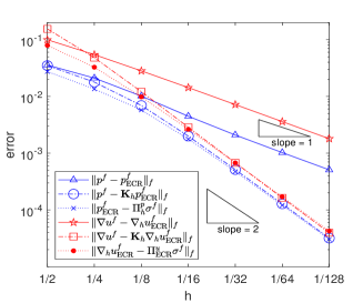
(b) ECR element

Figure 1: Errors of CR element and ECR element for the Stokes source problem.

4.2 Example 2

Consider the stokes eigenvalue problem (20) on unit domain. Since the exact eigenvalues are not known, we use element pair $(P_{3},P_{2})$ on $\mathcal{T}_{10}~{}(h=1/512)$ to compute the reference eigenvalues $\lambda_{1}=52.344691169,$ $\lambda_{2}=92.124393972$ and $\lambda_{3}=92.124393972,$ where $\lambda_{2}=\lambda_{3}$ are multiple eigenvalues. The relative errors of the first approximate eigenvalues of CR element, ECR element and their corresponding extrapolation eigenvalues on uniform triangulations $\mathcal{T}_{i}$ are presented in Table 1, and the error results of multiple eigenvalues are shown in Figure 2. Table 1 and Figure 2 show that extrapolation algorithm for the CR element and ECR element improves the convergence rate of both single eigenvalues and multiple eigenvalues to a higher rate 4. The numerical observation above directly verify the conclusions in Theorem 3.15 and its remark.

Table 1: The relative errors of the first eigenvalues and the extrapolation eigenvalues.

	$\lambda_{\mathrm{CR},1}$	rate	$\lambda_{\mathrm{CR},1}^{\mathrm{EXP}}$	rate	$\lambda_{\mathrm{ECR},1}$	rate	$\lambda_{\mathrm{ECR},1}^{\mathrm{EXP}}$	rate
$\mathcal{T}_{3}$	1.1808e-01	–	–	–	3.5002e-01	–	–	–
$\mathcal{T}_{4}$	3.2962e-02	1.84	4.5893e-03	–	9.0697e-02	1.95	4.2548e-03	–
$\mathcal{T}_{5}$	8.9271e-03	1.88	9.1544e-04	2.33	2.2723e-02	2.00	6.4759e-05	6.04
$\mathcal{T}_{6}$	2.3015e-03	1.96	9.3015e-05	3.30	5.7247e-03	1.99	5.8595e-05	0.14
$\mathcal{T}_{7}$	5.8063e-04	1.99	6.9912e-06	3.73	1.4354e-03	2.00	5.6166e-06	3.38
$\mathcal{T}_{8}$	1.4551e-04	2.00	4.7022e-07	3.89	3.5915e-04	2.00	4.0567e-07	3.79
$\mathcal{T}_{9}$	3.6400e-05	2.00	3.0000e-08	3.97	8.9807e-05	2.00	2.6000e-08	3.96

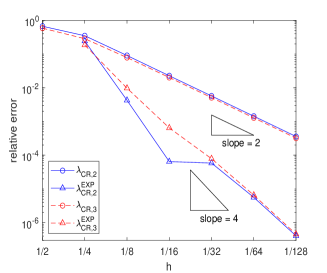
(a) CR element

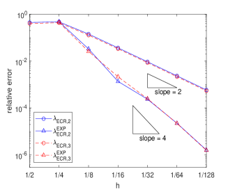
(b) ECR element

Figure 2: The relative errors of the multiple eigenvalues from CR element and ECR element.

References

• [1] Ivo M. Babuška and John E. Osborn. Eigenvalue problems. In Handbook of numerical analysis, Vol. II, volume II of Handb. Numer. Anal., pages 641–787. North-Holland, Amsterdam, 1991.
• [2] Heribert Blum and Rolf Rannacher. Finite element eigenvalue computation on domains with reentrant corners using Richardson extrapolation. J. Comput. Math., 8(4):321–332, 1990.
• [3] Jan H. Brandts. Superconvergence and a posteriori error estimation for triangular mixed finite elements. Numer. Math., 68(3):311–324, 1994.
• [4] Jan H. Brandts. Superconvergence for triangular order $k=1$ Raviart-Thomas mixed finite elements and for triangular standard quadratic finite element methods. Appl. Numer. Math., 34(1):39–58, 2000.
• [5] Jan H. Brandts and Michal Křížek. Gradient superconvergence on uniform simplicial partitions of polytopes. IMA J. Numer. Anal., 23(3):489–505, 2003.
• [6] Carsten Carstensen, Dietmar Gallistl, and Mira Schedensack. Quasi-optimal adaptive pseudostress approximation of the Stokes equations. SIAM J. Numer. Anal., 51(3):1715–1734, 2013.
• [7] Chuanmiao Chen and Yungqing Huang. High Accuracy Theory of Finite Element Methods. Hunan Science and Technology Press, Changsha, 1995.
• [8] Hongsen Chen and Bo Li. Superconvergence analysis and error expansion for the Wilson nonconforming finite element. Numer. Math., 69(2):125–140, 1994.
• [9] Wei Chen and Qun Lin. Approximation of an eigenvalue problem associated with the Stokes problem by the stream function-vorticity-pressure method. Appl. Math., 51(1):73–88, 2006.
• [10] Wei Chen and Qun Lin. Asymptotic expansion and extrapolation for the eigenvalue approximation of the biharmonic eigenvalue problem by Ciarlet-Raviart scheme. Adv. Comput. Math., 27(1):95–106, 2007.
• [11] Xi Chen and Yuwen Li. Superconvergent pseudostress-velocity finite element methods for the Oseen equations. J. Sci. Comput., 92(1):Paper No. 17, 27, 2022.
• [12] Philippe G. Ciarlet. The finite element method for elliptic problems, volume Vol. 4 of Studies in Mathematics and its Applications. North-Holland Publishing Co., Amsterdam-New York-Oxford, 1978.
• [13] Michel Crouzeix and Pierre-Arnaud Raviart. Conforming and nonconforming finite element methods for solving the stationary Stokes equations. I. Rev. Française Automat. Informat. Recherche Opérationnelle Sér. Rouge, 7:33–75, 1973.
• [14] Yanheng Ding and Qun Lin. Quadrature and extrapolation for the variable coefficient elliptic eigenvalue problem. Systems Sci. Math. Sci., 3(4):327–336, 1990.
• [15] Jim Douglas, Jr. and Jean E. Roberts. Global estimates for mixed methods for second order elliptic equations. Math. Comp., 44(169):39–52, 1985.
• [16] Jim Douglas, Jr. and Junping Wang. Superconvergence of mixed finite element methods on rectangular domains. Calcolo, 26(2-4):121–133, 1989.
• [17] Ricardo Durán. Superconvergence for rectangular mixed finite elements. Numer. Math., 58(3):287–298, 1990.
• [18] Hagen Eichel, Lutz Tobiska, and Hehu Xie. Supercloseness and superconvergence of stabilized low-order finite element discretizations of the Stokes problem. Math. Comp., 80(274):697–722, 2011.
• [19] Giovanni Paolo Galdi, Christian G. Simader, and Hermann Sohr. On the Stokes problem in Lipschitz domains. Ann. Mat. Pura Appl. (4), 167:147–163, 1994.
• [20] Jun Hu, Yunqing Huang, and Qun Lin. Lower bounds for eigenvalues of elliptic operators: by nonconforming finite element methods. J. Sci. Comput., 61(1):196–221, 2014.
• [21] Jun Hu, Yunqing Huang, and Quan Shen. The lower/upper bound property of approximate eigenvalues by nonconforming finite element methods for elliptic operators. J. Sci. Comput., 58(3):574–591, 2014.
• [22] Jun Hu and Limin Ma. Asymptotically exact a posteriori error estimates of eigenvalues by the Crouzeix-Raviart element and enriched Crouzeix-Raviart element. SIAM J. Sci. Comput., 42(2):A797–A821, 2020.
• [23] Jun Hu and Limin Ma. Asymptotic expansions of eigenvalues by both the Crouzeix-Raviart and enriched Crouzeix-Raviart elements. Math. Comp., 91(333):75–109, 2021.
• [24] Jun Hu and Rui Ma. The enriched Crouzeix-Raviart elements are equivalent to the Raviart-Thomas elements. J. Sci. Comput., 63(2):410–425, 2015.
• [25] Jun Hu and Zhongci Shi. A lower bound of the $L^{2}$ norm error estimate for the Adini element of the biharmonic equation. SIAM J. Numer. Anal., 51(5):2651–2659, 2013.
• [26] Hungtsai Huang, Zicai Li, and Qun Lin. New expansions of numerical eigenvalues by finite elements. J. Comput. Appl. Math., 217(1):9–27, 2008.
• [27] Yunqing Huang and Jinchao Xu. Superconvergence of quadratic finite elements on mildly structured grids. Math. Comp., 77(263):1253–1268, 2008.
• [28] Shanghui Jia, Fusheng Luo, and Hehu Xie. A posterior error analysis for the nonconforming discretization of Stokes eigenvalue problem. Acta Math. Sin. (Engl. Ser.), 30(6):949–967, 2014.
• [29] Shanghui Jia, Hehu Xie, Xiaobo Yin, and Shaoqin Gao. Approximation and eigenvalue extrapolation of biharmonic eigenvalue problem by nonconforming finite element methods. Numer. Methods Partial Differential Equations, 24(2):435–448, 2008.
• [30] Shanghui Jia, Hehu Xie, Xiaobo Yin, and Shaoqin Gao. Approximation and eigenvalue extrapolation of Stokes eigenvalue problem by nonconforming finite element methods. Appl. Math., 54(1):1–15, 2009.
• [31] Jiafu Lin and Qun Lin. Extrapolation of the Hood-Taylor elements for the Stokes problem. Adv. Comput. Math., 22(2):115–123, 2005.
• [32] Qun Lin, Hungtsai Huang, and Zicai Li. New expansions of numerical eigenvalues for $-\Delta u=\lambda\rho u$ by nonconforming elements. Math. Comp., 77(264):2061–2084, 2008.
• [33] Qun Lin, Hungtsai Huang, and Zicai Li. New expansions of numerical eigenvalues by Wilson’s element. J. Comput. Appl. Math., 225(1):213–226, 2009.
• [34] Qun Lin and Jiafu Lin. Finite Element Methods: Accuracy and Improvement. China Science Press, Beijing, 2006.
• [35] Qun Lin and Tao Lü. Asymptotic expansions for finite element eigenvalues and finite element solution. In Extrapolation procedures in the finite element method (Bonn, 1983), volume 158 of Bonner Math. Schriften, pages 1–10. Univ. Bonn, Bonn, 1984.
• [36] Qun Lin and Dongsheng Wu. High-accuracy approximations for eigenvalue problems by the Carey non-conforming finite element. Comm. Numer. Methods Engrg., 15(1):19–31, 1999.
• [37] Qun Lin and Hehu Xie. Asymptotic error expansion and Richardson extrapolation of eigenvalue approximations for second order elliptic problems by the mixed finite element method. Appl. Numer. Math., 59(8):1884–1893, 2009.
• [38] Qun Lin and Hehu Xie. New expansions of numerical eigenvalue for $-\Delta u=\lambda\rho u$ by linear elements on different triangular meshes. Int. J. Inf. Syst. Sci., 6(1):10–34, 2010.
• [39] Qun Lin, Hehu Xie, Fusheng Luo, Yu Li, and Yidu Yang. Stokes eigenvalue approximations from below with nonconforming mixed finite element methods. Math. Pract. Theory, 40(19):157–168, 2010.
• [40] Qun Lin, Junming Zhou, and Hongtao Chen. Extrapolation of three-dimensional eigenvalue finite element approximation. Math. Pract. Theory, 41(11):132–139, 2011.
• [41] Carlo Lovadina, Mikko Lyly, and Rolf Stenberg. A posteriori estimates for the Stokes eigenvalue problem. Numer. Methods Partial Differential Equations, 25(1):244–257, 2009.
• [42] Ping Luo and Qun Lin. High accuracy analysis of the Adini’s nonconforming element. Computing, 68(1):65–79, 2002.
• [43] Limin Ma and Shudan Tian. New fourth order postprocessing techniques for plate bending eigenvalues by Morley element. SIAM J. Sci. Comput., 44(4):B910–B937, 2022.
• [44] Shipeng Mao and Zhongci Shi. High accuracy analysis of two nonconforming plate elements. Numer. Math., 111(3):407–443, 2009.
• [45] Pierre-Arnaud Raviart and Jean-Marie Thomas. A mixed finite element method for 2nd order elliptic problems. In Mathematical aspects of finite element methods (Proc. Conf., Consiglio Naz. delle Ricerche (C.N.R.), Rome, 1975), volume Vol. 606 of Lecture Notes in Math., pages 292–315. Springer, Berlin-New York, 1977.
• [46] Zhongci Shi, Bin Jiang, and Weimin Xue. A new superconvergence property of Wilson nonconforming finite element. Numer. Math., 78(2):259–268, 1997.
• [47] Xiaobo Yin, Hehu Xie, Shanghui Jia, and Shaoqin Gao. Asymptotic expansions and extrapolations of eigenvalues for the Stokes problem by mixed finite element methods. J. Comput. Appl. Math., 215(1):127–141, 2008.