Joint Transceiver Optimization for MmWave/THz MU-MIMO ISAC Systems

Abstract

In this paper, we consider the problem of joint transceiver design for millimeter wave (mmWave)/Terahertz (THz) multi-user MIMO integrated sensing and communication (ISAC) systems. Such a problem is formulated into a nonconvex optimization problem, with the objective of maximizing a weighted sum of communication users’ rates and the passive radar’s signal-to-clutter-and-noise-ratio (SCNR). By exploring a low-dimensional subspace property of the optimal precoder, a low-complexity block-coordinate-descent (BCD)-based algorithm is proposed. Our analysis reveals that the hybrid analog/digital beamforming structure can attain the same performance as that of a fully digital precoder, provided that the number of radio frequency (RF) chains is no less than the number of resolvable signal paths. Also, through expressing the precoder as a sum of a communication-precoder and a sensing-precoder, we develop an analytical solution to the joint transceiver design problem by generalizing the idea of block-diagonalization (BD) to the ISAC system. Simulation results show that with a proper tradeoff parameter, the proposed methods can achieve a decent compromise between communication and sensing, where the performance of each communication/sensing task experiences only a mild performance loss as compared with the performance attained by optimizing exclusively for a single task.

I Introduction

The sixth generation (6G) wireless network is envisioned to support not only full-dimensional wireless connectivity but also enhanced sensing capabilities [1, 2]. Wireless communication and radar sensing have flourished as different disciplines due to their different objectives. Recently, with the development of millimeter-wave (mmWave)/terahertz (THz) communications as well as large-scale antenna arrays, mmWave/THz communication systems and radar sensing systems are now sharing many similarities in hardware structures, channel characteristics and signal processing techniques. Consequently, integrated sensing and communication (ISAC) is emerging as a paradigm-shifting concept with a great potential in revolutionizing both fields [3, 4].

Joint transceiver design is a key problem in mmWave/THz ISAC systems due to the inevitable competition for communication and sensing resources and the subsequent interference management [3, 5]. For mmWave and THz communications, massive antennas are employed at the base station (BS) and/or user equipments (UE) to compensate for the severe path loss incurred by mmWave/THz signals. Moreover, due to hardware and power constraints, hybrid analog and digital structures with a small number of radio frequency (RF) chains are usually adopted [6, 7, 8, 1, 2]. The large-scale antenna array along with a hybrid precoder/combiner structure makes joint transceiver design for ISAC systems a challenging problem. In addition, as the joint transceiver design has to be performed for each interval of channel coherence time that could be less than several milliseconds [9], low-complexity transceiver optimization algorithms are highly desirable in practical systems.

A plethora of studies [10, 11, 12, 13, 14, 15, 16, 17, 18] have been made to jointly devising transmit precoder and receive combiner for mmWave/THz ISAC systems. The existing body of literature can be roughly classified into three categories based on their design criteria. Communication-oriented approaches put their priority on communication tasks and try to improve the sensing accuracy given that the communication performance is guaranteed. Meanwhile, sensing-oriented approaches [14, 15] attempt to optimize the communication performance given that a certain sensing performance is attained. In addition to these approaches, some other works [16, 17, 19, 18] attempt to achieve a decent tradeoff between communication and sensing performance without explicitly considering any performance constraints on sensing or communication. Among them, [16, 17] proposed to find a precoder for mmWave/THz ISAC systems such that the precoder is as close as possible to the optimal precoder for communication and also as close as possible to the optimal precoder for sensing. Other tradeoffs between communication and sensing were also exploited. For instance, [19] proposed to optimize the tradeoff between the weighted sum rate (WSR) and the radar beam pattern matching error, while [18] aimed to maximize the sum of communication and sensing signal-to-noise-ratios (SNRs).

In this paper, we consider the problem of joint transceiver design for mmWave/THz multi-user MIMO ISAC systems, where a multi-antenna base station (BS) serves multiple users and a passive radar receiver is deployed to detect targets by processing reflections from BS’s downlink communication signals. Our objective is to optimize the transmit precoder along with the receive combiner such that the communication and sensing performance can be well compromised. To more accurately characterize the communication and sensing performance, a metric in terms of users’ weighted sum rate is used to evaluate the communication performance and a metric in terms of the signal-to-clutter-and-noise-ratio (SCNR) is used to evaluate the sensing performance. We aim at maximizing the sum of communication users’ sum rate and the radar’s received SCNR subject to a certain unit modulus and transmit power constraints. To tackle such a non-convex optimization problem, we propose two solutions, namely, a block-coordinate-descent (BCD)-based method which alternatively optimizes each block variable given other variables fixed, and an analytical solution that generalizes the block-diagonalization (BD) idea to the ISAC systems for joint transceiver design. Both methods enjoy a low computational complexity that scales linearly with the number of antennas at the BS. Specifically, a low-dimensional subspace property associated with the optimal precoder is explored to reduce the complexity of the BCD method. In addition, this low-dimensional subspace property also sheds light on the minimum number of RF chains that is required to achieve a fully-digital precoding performance for ISAC systems.

The rest of paper is organized as follows. In Section II, the system model and the problem formulation are discussed. In Section III, by exploring the low-dimensional subspace property, the BCD-based method is developed for joint transceiver design. Next, a simple analytical joint transceiver design method is proposed in Section IV. Simulation results are provided in Section V, followed by concluding remarks in Section VI.

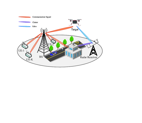
Figure 1: Illustration of mmWave/THz MU-MIMO ISAC systems

II System Model

In this paper, we consider an ISAC system where a multi-antenna BS serves $K$ multi-antenna UEs, and a passive radar receiver is deployed to detect a point-like target by processing reflections from BS’s downlink communication signals. To avoid self-interference, we consider a bistatic setup where the BS and the radar receiver are geographically separated (see Fig. 1). The BS and the radar are cable-connected such that they can exchange necessary information to facilitate detection and tracking of the target.

To reduce the hardware cost, we consider a hybrid analog and digital structure at both the BS and UEs. Specifically, the BS is equipped with $N_{t}$ antennas and $N_{t}^{\rm RF}$ radio frequency (RF) chains, and each UE is equipped with $N_{r}$ antennas and $N_{r}^{\rm RF}$ RF chains. The BS first employs a digital precoder $\boldsymbol{F}_{{\rm BB},k}\in\mathbb{C}^{N_{t}^{\rm RF}\times N_{s}}$ to precode the $k$th user’s transmitted symbol $\boldsymbol{s}_{k}\in\mathbb{C}^{N_{s}}$, where $N_{s}$ denotes the number of data streams and the transmitted symbol $\boldsymbol{s}_{k}$ is assumed to satisfy $\mathbb{E}[\boldsymbol{s}_{k}\boldsymbol{s}_{k}^{H}]=\boldsymbol{I}_{N_{s}}$. The signal is then processed by an analog precoder $\boldsymbol{F}_{\rm RF}\in\mathbb{C}^{N_{t}\times N_{t}^{\rm RF}}$ with its elements satisfying unit modulus constraints. The baseband signal forwarded to the $k$th user can be written as $\boldsymbol{x}_{k}=\boldsymbol{F}_{\rm RF}\boldsymbol{F}_{{\rm BB},k}\boldsymbol{s}_{k}$, and the transmitted signal can be expressed as

$$\boldsymbol{x}=\sum_{k=1}^{K}\boldsymbol{F}_{k}\boldsymbol{s}_{k},$$ (1)

where $\boldsymbol{F}_{k}\triangleq\boldsymbol{F}_{\rm RF}\boldsymbol{F}_{{\rm BB},k}$, and the transmit power constraint is given by $\mathbb{E}[\|\boldsymbol{x}\|_{2}^{2}]=\sum_{k=1}^{K}\text{Tr}(\boldsymbol{F}_{k}\boldsymbol{F}_{k}^{H})\leq P_{t}$ with $P_{t}$ denoting the maximum transmit power.

II-A MU-MIMO Communication Performance

The transmitted signal arrives at the $k$th user via propagating through the channel between the BS and the $k$th UE $\boldsymbol{H}_{k}\in\mathbb{C}^{N_{r}\times N_{t}}$. Due to the small wavelength, mmWave/THz channels exhibit sparse scattering characteristics and can be characterized by the Saleh-Valenzuela (S-V) model [9, 1]. Suppose both the BS and the UE are equipped with uniform linear arrays (ULA), $\boldsymbol{H}_{k}$ can be modeled as

$$\boldsymbol{H}_{k}=\sum_{l_{k}=1}^{L_{k}}\beta_{l_{k}}\boldsymbol{a}_{r}(\gamma_{l_{k}})\boldsymbol{a}_{t}^{H}(\varphi_{l_{k}}),$$ (2)

where $L_{k}$ denotes the total number of signal paths, $\beta_{l_{k}}$ is the complex gain associated with the $l_{k}$th path, $\varphi_{l_{k}}$ and $\gamma_{l_{k}}$ respectively denote the angle-of-departure (AoD) and the angle-of-arrival (AoA) associated with the $l_{k}$th path, $\boldsymbol{a}_{r}(\cdot)$ and $\boldsymbol{a}_{t}(\cdot)$ denote the normalized receive and transmit array steering vectors at the UE and the BS, respectively.

The signal received by the $k$th UE is given by

$$\bar{\boldsymbol{y}}_{k}=\boldsymbol{H}_{k}\boldsymbol{F}_{k}\boldsymbol{s}_{k}+\sum_{j\neq k}^{K}\boldsymbol{H}_{k}\boldsymbol{F}_{j}\boldsymbol{s}_{j}+\boldsymbol{n}_{k},$$ (3)

where $\boldsymbol{n}_{k}\sim\mathcal{CN}(0,\sigma_{k}^{2}\boldsymbol{I})$ is the additive white Gaussian noise (AWGN). The received signal is first processed by an analog combiner $\boldsymbol{W}_{{\rm RF},k}\in\mathbb{C}^{N_{r}\times N_{r}^{\rm RF}}$ and then followed by a lower-dimensional digital combiner $\boldsymbol{W}_{{\rm BB},k}\in\mathbb{C}^{N_{r}^{\rm RF}\times N_{s}}$. Define $\boldsymbol{W}_{k}\triangleq\boldsymbol{W}_{{\rm RF},k}\boldsymbol{W}_{{\rm BB},k}\in\mathbb{C}^{N_{r}\times N_{s}}$, the received baseband signal is thus given as

$$\boldsymbol{y}_{k}=\boldsymbol{W}_{k}^{H}\boldsymbol{H}_{k}\boldsymbol{F}_{k}\boldsymbol{s}_{k}+\sum_{j\neq k}^{K}\boldsymbol{W}_{k}^{H}\boldsymbol{H}_{k}\boldsymbol{F}_{j}\boldsymbol{s}_{j}+\boldsymbol{W}_{k}^{H}\boldsymbol{n}_{k}.$$ (4)

Accordingly, the achievable rate of the $k$th user is given by

$$R_{k}=\log_{2}{\rm det}\left(\boldsymbol{I}+\boldsymbol{W}_{k}^{H}\boldsymbol{H}_{k}\boldsymbol{F}_{k}\boldsymbol{F}_{k}^{H}\boldsymbol{H}_{k}^{H}\boldsymbol{W}_{k}\boldsymbol{J}_{k}^{-1}\right),$$ (5)

where

$$\boldsymbol{J}_{k}\triangleq\sum_{j\neq k}^{K}\boldsymbol{W}_{k}^{H}\boldsymbol{H}_{k}\boldsymbol{F}_{j}\boldsymbol{F}_{j}^{H}\boldsymbol{H}_{k}^{H}\boldsymbol{W}_{k}+\sigma_{k}^{2}\boldsymbol{W}_{k}^{H}\boldsymbol{W}_{k}.$$ (6)

The WSR can be calculated as

$$R(\boldsymbol{F}_{k},\boldsymbol{W}_{k})=\sum_{k=1}^{K}w_{k}R_{k},$$ (7)

where $w_{k}$ denotes a weight characterizing the priority of the $k$th UE. Note that the system parameters satisfy $KN_{s}\leq N_{t}^{\rm RF}\leq N_{t}$ and $N_{s}\leq N_{r}^{\rm RF}\leq N_{r}$.

II-B MIMO Sensing Performance

The radar receiver is equipped with $N_{\rm sen}$ antennas. Assuming a point-like target is located at angle $\theta_{0}$ with respect to (w.r.t.) the BS and angle $\varphi_{0}$ w.r.t the radar receiver, the target response matrix is expressed as

$$\boldsymbol{H}_{A}=\alpha_{0}\boldsymbol{a}_{s}(\varphi_{0})\boldsymbol{a}_{t}^{H}(\theta_{0}),$$ (8)

where $\boldsymbol{a}_{s}(\cdot)\in\mathbb{C}^{N_{\rm sen}}$ denotes the normalized receive array steering vector at the radar receiver, $\alpha_{0}$ is the complex gain incorporating the target radar cross section (RCS) as well as the path loss. Here, $\alpha_{0}$ is assumed to be a zero mean complex Gaussian random variable with variance $\sigma_{A}^{2}$ [5]. In addition to the echo back-scattered from the target, the radar receiver also receives echoes from the environment [5, 20], i.e., the clutter. Suppose there are $I$ clutter patches . The response matrix associated with the $i$th clutter is given as

$$\boldsymbol{H}_{B,i}=\alpha_{i}\boldsymbol{a}_{s}(\varphi_{i})\boldsymbol{a}_{t}^{H}(\theta_{i}),$$ (9)

where $\alpha_{i}\sim\mathcal{CN}(0,\sigma_{B_{i}}^{2})$ is the complex gain associated with the $i$th clutter patch, $\varphi_{i}$ and $\theta_{i}$ denote the AoA and AoD at the radar receiver and BS, respectively. The received signal at the radar receiver is given by

$$\boldsymbol{y}_{0}= \boldsymbol{H}_{A}\boldsymbol{x}+\sum_{i=1}^{I}\boldsymbol{H}_{B,i}\boldsymbol{x}+\boldsymbol{n}_{0},$$ (10)

where $\boldsymbol{x}$ is the communication signal defined in (1), and $\boldsymbol{n}_{0}\in\mathbb{C}^{N_{\rm sen}\times 1}$ is the AWGN satisfying $\mathcal{CN}(0,\sigma^{2}\boldsymbol{I})$.

Let $\boldsymbol{w}\in\mathbb{C}^{N_{\rm sen}}$ denote the radar receive beamforming vector. The output of the radar receiver is given by

$$r=\boldsymbol{w}^{H}\boldsymbol{y}_{0}=\boldsymbol{w}^{H}\boldsymbol{H}_{A}\boldsymbol{x}+\boldsymbol{w}^{H}\sum_{i=1}^{I}\boldsymbol{H}_{B,i}\boldsymbol{x}+\boldsymbol{w}^{H}\boldsymbol{n}_{0}.$$ (11)

For sensing tasks, the SCNR determines both detection and localization performance [5, 20]. Therefore we use SCNR as a metric to evaluate the sensing performance. Specifically, the SCNR is defined as the ratio of the average received signal power to the average received clutter power plus the noise power [5, 14], i.e.,

$${\text{SCNR}}(\boldsymbol{w},\boldsymbol{F}_{k})\stackrel{{\scriptstyle(a)}}{{=}} \frac{\mathbb{E}[|\boldsymbol{w}^{H}\boldsymbol{H}_{A}\boldsymbol{x}|^{2}]}{\mathbb{E}[|\boldsymbol{w}^{H}\sum_{i=1}^{I}\boldsymbol{H}_{B,i}\boldsymbol{x}+\boldsymbol{w}^{H}\boldsymbol{n}_{0}|^{2}]}$$

$$= \frac{\boldsymbol{w}^{H}\boldsymbol{A}\boldsymbol{F}\boldsymbol{F}^{H}\boldsymbol{A}^{H}\boldsymbol{w}}{\boldsymbol{w}^{H}\left(\sum_{i=1}^{I}\boldsymbol{B}_{i}\boldsymbol{F}\boldsymbol{F}^{H}\boldsymbol{B}_{i}^{H}+\sigma^{2}\boldsymbol{I}\right)\boldsymbol{w}},$$ (12)

where the expectation in $(a)$ is taken over the transmitted signal $\boldsymbol{x}$ as well as the random target/clutter response matrices, and $\boldsymbol{A}$, $\boldsymbol{B}_{i}$ and $\boldsymbol{F}$ are respectively defined as

$$\boldsymbol{A}= \sigma_{A}\boldsymbol{a}_{s}(\varphi_{0})\boldsymbol{a}_{t}^{H}(\theta_{0}),$$ (13)

$$\boldsymbol{B}_{i}= \sigma_{B_{i}}\boldsymbol{a}_{s}(\varphi_{i})\boldsymbol{a}_{t}^{H}(\theta_{i}),\forall i$$ (14)

$$\boldsymbol{F}= [\boldsymbol{F}_{1}\phantom{0}\boldsymbol{F}_{2}\ldots\boldsymbol{F}_{K}]\in\mathbb{C}^{N_{t}\times KN_{s}}.$$ (15)

Note that the statistical information of the target and the clutter patches $\{\sigma_{A}^{2},\sigma_{B,i}^{2}\}$ are assumed known a priori. In practice, they can be estimated based on a cognitive paradigm [21].

II-C Problem Formulation

As discussed earlier, the communication performance is measured by the WSR while the sensing performance is determined by the SCNR. In this paper, we hope to achieve a tradeoff between the communication and sensing performance by jointly optimizing the hybrid precoder/combiner $\{\boldsymbol{F}_{k},\boldsymbol{W}_{k}\}$ and the radar receive beamforming vector $\boldsymbol{w}$. The optimization problem can be formulated as

$$\max_{\{\boldsymbol{F}_{k},\boldsymbol{W}_{k}\}_{k=1}^{K},\boldsymbol{w}}\quad \rho_{c}R(\boldsymbol{F}_{k},\boldsymbol{W}_{k})+\rho_{s}\text{SCNR}(\boldsymbol{w},\boldsymbol{F}_{k})$$

s.t. $$\sum_{k=1}^{K}{\rm tr}(\boldsymbol{F}_{k}\boldsymbol{F}_{k}^{H})\leq P_{t},$$

$$\boldsymbol{F}_{k}=\boldsymbol{F}_{\rm RF}\boldsymbol{F}_{{\rm BB},k},$$

$$\boldsymbol{W}_{k}=\boldsymbol{W}_{{\rm RF},k}\boldsymbol{W}_{{\rm BB},k},$$

$$|(\boldsymbol{F}_{\rm RF})_{i,j}|=1,$$

$$|(\boldsymbol{W}_{\rm RF})_{i,j}|=1,$$ (16)

where $R(\boldsymbol{F}_{k},\boldsymbol{W}_{k})$ is defined in (7), ${\text{SCNR}}(\boldsymbol{w},\boldsymbol{F}_{k})$ is defined in (12). The weighting coefficients $\rho_{c}=\frac{\eta}{\text{cons}_{1}},\rho_{s}=\frac{1-\eta}{\text{cons}_{2}}$ are used to control the tradeoff between communication and sensing performance, in which $\text{cons}_{1}$ and $\text{cons}_{2}$ are predefined constants used to reduce the weighting effects caused by the large difference in values between SCNR and WSR. When $\eta=1$, the system focuses only on the communication performance. On the contrary, when $\eta=0$, the sensing performance is exclusively optimized. As $\eta$ varies from 0 to 1, the performance tradeoff can be characterized by the optimal solution of (16).

The optimization problem (16) is challenging due to its nonconvexity as well as coupling among optimization variables. In the following, we propose a low-complexity block-coordinated descent-based method to solve (16).

III Proposed BCD-Based Method

For simplicity, we first ignore the constraints placed by the hybrid structure at the transceiver and consider a fully digital precoder/combiner $\boldsymbol{F}_{k}$/$\boldsymbol{W}_{k}$. After the optimal fully digital precoder/combiner is obtained, an efficient manifold optimization-based algorithm is employed to find hybrid precoder/combiner to approximate the optimal digital precoder/combiner.

III-A Problem Reformulation

By ignoring the constraint imposed by hybrid structures, the problem (16) is simplified as

$$\max_{\{\boldsymbol{F}_{k},\boldsymbol{W}_{k}\}_{k=1}^{K},\boldsymbol{w}}\quad \rho_{c}R(\boldsymbol{F}_{k},\boldsymbol{W}_{k})+\rho_{s}\text{SCNR}(\boldsymbol{w},\boldsymbol{F}_{k})$$

s.t. $$\sum_{k=1}^{K}{\rm tr}(\boldsymbol{F}_{k}\boldsymbol{F}_{k}^{H})\leq P_{t}.$$ (17)

Before proceeding, we consider the problem of optimizing $\{\boldsymbol{F}_{k}\}_{k=1}^{K}$, given fixed $\{\boldsymbol{W}\}_{k=1}^{K}$ and $\boldsymbol{w}$, in which case the problem becomes

$$\max_{\{\boldsymbol{F}_{k}\}_{k=1}^{K}}\quad \rho_{c}R(\boldsymbol{F}_{k},\boldsymbol{W}_{k})+\rho_{s}\text{SCNR}(\boldsymbol{w},\boldsymbol{F}_{k})$$

s.t. $$\sum_{k=1}^{K}{\rm tr}(\boldsymbol{F}_{k}\boldsymbol{F}_{k}^{H})\leq P_{t}.$$ (18)

We first obtain an interesting and useful result regarding the low-dimensional subspace property of $\{\boldsymbol{F}_{k}\}_{k=1}^{K}$ by exploiting the sparse characteristics of mmWave/THz channels.

Proposition 1

Denote

$$\boldsymbol{V}= [\boldsymbol{a}_{t}(\varphi_{1})\ldots\boldsymbol{a}_{t}(\varphi_{L_{K}})\phantom{0}\boldsymbol{a}_{t}(\theta_{0})\phantom{0}\boldsymbol{a}_{t}(\theta_{1})\ldots\boldsymbol{a}_{t}(\theta_{I})]\in\mathbb{C}^{N_{t}\times r}$$ (19)

as the matrix consisting of the steering vectors from the BS to all UEs, the steering vectors from the BS to the target and the steering vectors from the BS to all clutter patches, where we have $r\triangleq\sum_{k=1}^{K}L_{k}+I+1$. Then, any non-trivial Karush-Kuhn-Tucker (KKT) point of (18) can be expressed as

$$\boldsymbol{F}_{k}=\boldsymbol{V}\boldsymbol{X}_{k},\quad\forall k$$ (20)

where $\boldsymbol{X}_{k}\in\mathbb{C}^{r\times N_{s}}$.

Proof:

See Appendix A. ∎

Define

$$\boldsymbol{H}\triangleq [\boldsymbol{H}_{1}^{T}\phantom{0}\ldots\phantom{0}\boldsymbol{H}_{K}^{T}\phantom{0}\boldsymbol{A}^{T}\phantom{0}\boldsymbol{B}_{1}^{T}\phantom{0}\ldots\phantom{0}\boldsymbol{B}_{I}^{T}]^{T}\in\mathbb{C}^{M\times N_{t}},$$ (21)

where $M=KN_{r}+(I+1)N_{\rm sen}$. It can be readily verified that $\boldsymbol{V}$ and $\boldsymbol{H}^{H}$ have the same range space, i.e., $\mathcal{R}(\boldsymbol{V})=\mathcal{R}(\boldsymbol{H}^{H})$. The low-dimensional subspace property for communication systems has been verified by classical linear precoders [22], e.g., the maximum-ratio-transmission (MRT) precoder $\boldsymbol{F}_{\rm MRT}=\boldsymbol{H}^{H}$ and the zero-forcing (ZF) precoder $\boldsymbol{F}_{\rm ZF}=\boldsymbol{H}^{H}(\boldsymbol{H}\boldsymbol{H}^{H})^{-1}$. Here, we show that the precoder $\boldsymbol{F}$ for ISAC systems also exhibits this intriguing low-dimensional subspace property.

Define $\bar{\boldsymbol{H}}_{k}\triangleq\boldsymbol{H}_{k}\boldsymbol{V}\in\mathbb{C}^{N_{r}\times r}$, $\bar{\boldsymbol{A}}\triangleq\boldsymbol{A}\boldsymbol{V}\in\mathbb{C}^{N_{\rm sen}\times r}$, $\bar{\boldsymbol{B}}_{i}\triangleq\boldsymbol{B}_{i}\boldsymbol{V}\in\mathbb{C}^{N_{\rm sen}\times r}$, $\tilde{\boldsymbol{H}}\triangleq\boldsymbol{V}^{H}\boldsymbol{V}\in\mathbb{C}^{r\times r}$. By invoking Proposition 1, the problem (17) can be rewritten as

$$\max_{\{\boldsymbol{X}_{k},\boldsymbol{W}_{k}\}_{k=1}^{K},\boldsymbol{w}}\quad \rho_{c}R(\boldsymbol{X}_{k},\boldsymbol{W}_{k})+\rho_{s}\text{SCNR}(\boldsymbol{w},\boldsymbol{X}_{k})$$

s.t. $$\sum_{k=1}^{K}{\rm tr}(\tilde{\boldsymbol{H}}\boldsymbol{X}_{k}\boldsymbol{X}_{k}^{H})\leq P_{t}.$$ (22)

where

$$R(\boldsymbol{X}_{k},\boldsymbol{W}_{k})$$

$$= \sum_{k=1}^{K}w_{k}\log_{2}{\rm det}\bigg{(}\boldsymbol{I}+\boldsymbol{W}_{k}^{H}\bar{\boldsymbol{H}}_{k}\boldsymbol{X}_{k}\boldsymbol{X}_{k}^{H}\bar{\boldsymbol{H}}_{k}^{H}\boldsymbol{W}_{k}$$

$$\times\big{(}\sum_{j\neq k}^{K}\boldsymbol{W}_{k}^{H}\bar{\boldsymbol{H}}_{k}\boldsymbol{X}_{j}\boldsymbol{X}_{j}^{H}\bar{\boldsymbol{H}}_{k}^{H}\boldsymbol{W}_{k}+\sigma_{k}^{2}\boldsymbol{W}_{k}^{H}\boldsymbol{W}_{k}\big{)}^{-1}\bigg{)},$$ (23)

and

$${\text{SCNR}}(\boldsymbol{w},\boldsymbol{X}_{k})=\frac{\boldsymbol{w}^{H}\bar{\boldsymbol{A}}\boldsymbol{X}\boldsymbol{X}^{H}\bar{\boldsymbol{A}}^{H}\boldsymbol{w}}{\boldsymbol{w}^{H}\left(\sum_{i=1}^{I}\bar{\boldsymbol{B}}_{i}{\boldsymbol{X}}\boldsymbol{X}^{H}\bar{\boldsymbol{B}}_{i}^{H}+\sigma^{2}\boldsymbol{I}\right)\boldsymbol{w}}$$ (24)

in which $\boldsymbol{X}\triangleq[\boldsymbol{X}_{1}\phantom{0}\ldots\phantom{0}\boldsymbol{X}_{K}]\in\mathbb{C}^{r\times KN_{s}}$.

In (22), the optimization variable $\boldsymbol{F}\in\mathbb{C}^{N_{t}\times KN_{s}}$ is replaced by $\boldsymbol{X}\in\mathbb{C}^{r\times KN_{s}}$. Note that, due to limited scattering characteristics of mmWave/THz signals, the dimension $r$ is usually smaller than the number of antennas $N_{t}$ at the BS. As a result, Proposition 1 allows us to remarkably reduce the complexity of the proposed algorithm, as will be elaborated in Section III-B.

Furthermore, it should be noted that the optimal solution to (22) will always be on the boundary of the quadratic constraint, which is known as the full power property. Using this property, the constraint in (22) can be removed and absorbed into the objective function, which yields

$$\max_{\{\boldsymbol{X}_{k},\boldsymbol{W}_{k}\}_{k=1}^{K},\boldsymbol{w}}\quad \rho_{c}\bar{R}(\boldsymbol{X}_{k},\boldsymbol{W}_{k})+\rho_{s}\overline{\text{SCNR}}(\boldsymbol{w},\boldsymbol{X}_{k}),$$ (25)

where

$$\bar{R}(\boldsymbol{X}_{k},\boldsymbol{W}_{k})$$

$$= \sum_{k=1}^{K}w_{k}\log_{2}{\rm det}\bigg{(}\boldsymbol{I}+\boldsymbol{W}_{k}^{H}\bar{\boldsymbol{H}}_{k}\boldsymbol{X}_{k}\boldsymbol{X}_{k}^{H}\bar{\boldsymbol{H}}_{k}^{H}\boldsymbol{W}_{k}$$

$$\times\bigg{(}\sum_{j\neq k}^{K}\boldsymbol{W}_{k}^{H}\bar{\boldsymbol{H}}_{k}\boldsymbol{X}_{j}\boldsymbol{X}_{j}^{H}\bar{\boldsymbol{H}}_{k}^{H}\boldsymbol{W}_{k}$$

$$+\frac{\sigma_{k}^{2}}{P_{t}}\sum_{i=1}^{K}{\rm tr}(\tilde{\boldsymbol{H}}\boldsymbol{X}_{i}\boldsymbol{X}_{i}^{H})\boldsymbol{W}_{k}^{H}\boldsymbol{W}_{k}\bigg{)}^{-1}\bigg{)},$$ (26)

and

$$\overline{\text{SCNR}}(\boldsymbol{w},\boldsymbol{X}_{k})$$

$$= \frac{\boldsymbol{w}^{H}\bar{\boldsymbol{A}}\boldsymbol{X}\boldsymbol{X}^{H}\bar{\boldsymbol{A}}^{H}\boldsymbol{w}}{\boldsymbol{w}^{H}\left(\sum_{i=1}^{I}(\bar{\boldsymbol{B}}_{i}{\boldsymbol{X}}\boldsymbol{X}^{H}\bar{\boldsymbol{B}}_{i}^{H})+\frac{\sigma^{2}}{P_{t}}\sum_{i=1}^{K}{\rm tr}(\tilde{\boldsymbol{H}}\boldsymbol{X}_{i}\boldsymbol{X}_{i}^{H})\boldsymbol{I}_{r}\right)\boldsymbol{w}}.$$ (27)

Next, we show that the optimal solution of (22) can be obtained by solving (25).

Proposition 2

Denote $(\{\boldsymbol{W}_{k}^{\rm opt_{1}},\boldsymbol{X}_{k}^{\rm opt_{1}}\}_{k=1}^{K},\boldsymbol{w}^{\rm opt_{1}})$ as the optimal solution to (22) and $(\{\boldsymbol{W}_{k}^{\rm opt_{2}},\boldsymbol{X}_{k}^{\rm opt_{2}}\}_{k=1}^{K},\boldsymbol{w}^{\rm opt_{2}})$ as the optimal solution to (25). Then, we have

$$\boldsymbol{W}_{k}^{\rm opt_{1}}=\boldsymbol{W}_{k}^{\rm opt_{2}},\boldsymbol{w}^{\rm opt_{1}}=\boldsymbol{w}^{\rm opt_{2}},\boldsymbol{X}_{k}^{\rm opt_{1}}=\alpha\boldsymbol{X}_{k}^{\rm opt_{2}},\forall k,$$ (28)

where

$$\alpha=\sqrt{\frac{P_{t}}{\sum_{k=1}^{K}{\rm tr}(\tilde{\boldsymbol{H}}\boldsymbol{X}_{k}^{\rm opt_{2}}(\boldsymbol{X}_{k}^{\rm opt_{2}})^{H})}}.$$ (29)

Proof:

See Appendix B. ∎

So far we have converted the problem (17) into a low-dimensional unconstrained problem (25). Nevertheless, it is still difficult to solve (25) due to coupling among optimization variables. To address this issue, we use the following tricks to simplify the WSR term and the SCNR term. Specifically, by resorting to the WMMSE technique[22], the WSR term $\bar{R}(\boldsymbol{X}_{k},\boldsymbol{W}_{k})$ in (26) can be formulated into the following optimization:

$$\bar{R}(\boldsymbol{X}_{k},\boldsymbol{W}_{k})$$

$$= \max_{\boldsymbol{\Lambda}_{k}\succ 0,\boldsymbol{E}_{k}}\quad\sum_{k=1}^{K}w_{k}\bigg{(}\log_{2}{\rm det}(\boldsymbol{\Lambda}_{k})-{\rm tr}(\boldsymbol{\Lambda}_{k}\boldsymbol{E}_{k})\bigg{)}+KN_{s},$$ (30)

where $\{\boldsymbol{\Lambda}_{k}\}_{k=1}^{K}$ are auxiliary variables and

$$\boldsymbol{E}_{k}= (\boldsymbol{I}-\boldsymbol{W}_{k}^{H}\bar{\boldsymbol{H}}_{k}\boldsymbol{X}_{k})(\boldsymbol{I}-\boldsymbol{W}_{k}^{H}\bar{\boldsymbol{H}}_{k}\boldsymbol{X}_{k})^{H}$$

$$+\boldsymbol{W}_{k}\bar{\boldsymbol{J}_{k}}\boldsymbol{W}_{k}^{H},$$ (31)

in which

$$\bar{\boldsymbol{J}_{k}}= \sum_{j=1,j\neq k}^{K}\bar{\boldsymbol{H}}_{k}\boldsymbol{X}_{j}\boldsymbol{X}_{j}^{H}\bar{\boldsymbol{H}}_{k}^{H}+\frac{\sigma_{k}^{2}}{P_{t}}\sum_{i=1}^{K}{\rm tr}(\tilde{\boldsymbol{H}}\boldsymbol{X}_{i}\boldsymbol{X}_{i}^{H})\boldsymbol{I}.$$ (32)

On the other hand, the SCNR term can be written as

$$\frac{\boldsymbol{w}^{H}\bar{\boldsymbol{A}}\boldsymbol{X}\boldsymbol{X}^{H}\bar{\boldsymbol{A}}\boldsymbol{w}}{\boldsymbol{w}^{H}\left(\sum_{i=1}^{I}(\bar{\boldsymbol{B}}_{i}{\boldsymbol{X}}\boldsymbol{X}^{H}\bar{\boldsymbol{B}}_{i}^{H})+\frac{\sigma^{2}}{P_{t}}\sum_{i=1}^{K}{\rm tr}(\tilde{\boldsymbol{H}}\boldsymbol{X}_{i}\boldsymbol{X}_{i}^{H})\boldsymbol{I}\right)\boldsymbol{w}}$$

$$\triangleq \frac{f_{1}({\boldsymbol{X}},\boldsymbol{w})}{f_{2}({\boldsymbol{X}},\boldsymbol{w})}.$$ (33)

By introducing an auxiliary vector $\boldsymbol{u}=[\boldsymbol{u}_{1}^{T}\phantom{0}\boldsymbol{u}_{2}^{T}\phantom{0}\ldots\phantom{0}\boldsymbol{u}_{K}^{T}]^{T}\in\mathbb{C}^{KN_{s}}$ with $\boldsymbol{u}_{k}\in\mathbb{C}^{N_{s}}$, the SCNR term is equivalent to solving the following optimization [23]

$$\overline{\text{SCNR}}(\boldsymbol{w},\boldsymbol{X}_{k})=\max_{\boldsymbol{u}}\;2\Re\{\boldsymbol{w}^{H}\bar{\boldsymbol{A}}\boldsymbol{X}\boldsymbol{u}\}-\|\boldsymbol{u}\|_{2}^{2}f_{2}({\boldsymbol{X}},\boldsymbol{w}).$$ (34)

Combining (30) and (34), the problem (25) is finally simplified as

$$\min_{\{\boldsymbol{\Lambda}_{k},\boldsymbol{W}_{k},\boldsymbol{X}_{k}\}_{k=1}^{K},\boldsymbol{w},\boldsymbol{u}}\; \sum_{k=1}^{K}\rho_{c}w_{k}\left({\rm tr}\left(\boldsymbol{\Lambda}_{k}\boldsymbol{E}_{k}\right)-\log{\rm det}(\boldsymbol{\Lambda}_{k})\right)$$

$$-\rho_{s}\left(2\Re\{\boldsymbol{w}^{H}\bar{\boldsymbol{A}}\boldsymbol{X}\boldsymbol{u}\}-\|\boldsymbol{u}\|_{2}^{2}f_{2}(\boldsymbol{X},\boldsymbol{w})\right).$$ (35)

Although the objective function of (35) is nonconvex, it is convex over each individual optimization variable when the other variables are fixed. Hence, a block-coordinate-descent (BCD) method can be applied to solve the problem (35).

III-B The Proposed BCD-Based Algorithm

In the sequel, we update each block variable while fixing the others. Since each subproblem is convex, its optimal solution can be obtained in a closed-form by checking the first-order optimality condition. The details are given as follows.

III-B1 Update $\boldsymbol{w}$

Given other variables fixed, the optimization of $\boldsymbol{w}$ can be formulated as

$$\min_{\boldsymbol{w}}\quad-2\Re\{\boldsymbol{w}^{H}\boldsymbol{A}\boldsymbol{X}\boldsymbol{u}\}+\|\boldsymbol{u}\|_{2}^{2}f_{2}(\boldsymbol{X},\boldsymbol{w}),$$ (36)

where $f_{2}(\boldsymbol{X},\boldsymbol{w})$ is defined in (33). By checking its first-order optimality condition, we can update $\boldsymbol{w}$ via

$$\boldsymbol{w}= \frac{1}{\|\boldsymbol{u}\|_{2}^{2}}\left(\sum_{i=1}^{I}(\bar{\boldsymbol{B}}_{i}{\boldsymbol{X}}\boldsymbol{X}^{H}\bar{\boldsymbol{B}}_{i}^{H})+\frac{\sigma^{2}}{P_{t}}\sum_{k=1}^{K}{\rm tr}(\tilde{\boldsymbol{H}}\boldsymbol{X}_{k}\boldsymbol{X}_{k}^{H})\boldsymbol{I}\right)^{-1}$$

$$\times\bar{\boldsymbol{A}}\boldsymbol{X}\boldsymbol{u}.$$ (37)

III-B2 Update $\boldsymbol{W}_{k}$

Given other variables fixed, the optimization of $\boldsymbol{W}_{k}$ is simplified as

$$\min_{\boldsymbol{W}_{k}}\quad{\rm tr}(\boldsymbol{\Lambda}_{k}\boldsymbol{E}_{k}),$$ (38)

where $\boldsymbol{E}_{k}$ is defined in (31). Hence, the update of $\boldsymbol{W}_{k}$ is given by

$$\boldsymbol{W}_{k}= {\left(\sum_{i=1}^{K}\bar{\boldsymbol{H}}_{k}\boldsymbol{X}_{i}\boldsymbol{X}_{i}^{H}\bar{\boldsymbol{H}}_{k}^{H}+\frac{\sigma_{k}^{2}}{P_{t}}\sum_{i=1}^{K}{\rm tr}(\tilde{\boldsymbol{H}}\boldsymbol{X}_{i}\boldsymbol{X}_{i}^{H})\boldsymbol{I}\right)^{-1}}$$

$$\times\bar{\boldsymbol{H}}_{k}\boldsymbol{X}_{k}.$$ (39)

III-B3 Update $\boldsymbol{\Lambda}_{k}$

Given other variables fixed, the update of $\boldsymbol{\Lambda}_{k}$ is given by

$$\boldsymbol{\Lambda}_{k}=(\boldsymbol{I}-\boldsymbol{W}_{k}^{H}\bar{\boldsymbol{H}}_{k}\boldsymbol{X}_{k})^{-1}.$$ (40)

III-B4 Update $\boldsymbol{X}_{k}$

Given other variables fixed, the optimization of $\boldsymbol{X}_{k}$ is formulated as

$$\min_{\boldsymbol{X}_{k}}\; \sum_{k=1}^{K}\left(\rho_{c}w_{k}{\rm tr}\left(\boldsymbol{\Lambda}_{k}\boldsymbol{E}_{k}\right)\right)+\rho_{s}\|\boldsymbol{u}\|_{2}^{2}{\rm tr}(\boldsymbol{X}^{H}{\tilde{\boldsymbol{B}}}\boldsymbol{X})$$

$$-2\rho_{s}\Re\{\boldsymbol{w}^{H}\bar{\boldsymbol{A}}\boldsymbol{X}\boldsymbol{u}\}+\frac{\rho_{s}\sigma^{2}}{P_{t}}\|\boldsymbol{u}\|_{2}^{2}\|\boldsymbol{w}\|_{2}^{2}\sum_{i=1}^{K}{\rm tr}(\tilde{\boldsymbol{H}}\boldsymbol{X}_{i}\boldsymbol{X}_{i}^{H}),$$ (41)

where $\boldsymbol{E}_{k}$ is defined in (31) and $\tilde{\boldsymbol{B}}=\sum_{i=1}^{I}\bar{\boldsymbol{B}}_{i}^{H}\boldsymbol{w}\boldsymbol{w}^{H}\bar{\boldsymbol{B}}_{i}$. Similarly, by checking its first-order optimality condition, the update of $\boldsymbol{X}_{k}$ is given by

$$\boldsymbol{X}_{k}$$

$$= \bigg{(}\rho_{c}\sum_{i=1}^{K}w_{i}\bar{\boldsymbol{H}}_{i}^{H}\boldsymbol{W}_{i}\boldsymbol{\Lambda}_{i}\boldsymbol{W}_{i}^{H}\bar{\boldsymbol{H}}_{i}+\rho_{s}\|\boldsymbol{u}\|_{2}^{2}{\tilde{\boldsymbol{B}}}$$

$$+\bigg{(}\rho_{c}\sum_{i=1}^{K}\frac{w_{i}\sigma_{i}^{2}}{P_{t}}{\rm tr}(\boldsymbol{\Lambda}_{i}\boldsymbol{W}_{i}^{H}\boldsymbol{W}_{i})+\frac{\rho_{s}\sigma^{2}}{P_{t}}\|\boldsymbol{u}\|_{2}^{2}\|\boldsymbol{w}\|_{2}^{2}\bigg{)}\tilde{\boldsymbol{H}}\bigg{)}^{-1}$$

$$\times\left(\rho_{c}w_{k}\bar{\boldsymbol{H}}_{k}^{H}\boldsymbol{W}_{k}\boldsymbol{\Lambda}_{k}+\rho_{s}\bar{\boldsymbol{A}}^{H}\boldsymbol{w}\boldsymbol{u}_{k}^{H}\right).$$ (42)

III-B5 Update $\boldsymbol{u}_{k}$

Given other variables fixed, we can update $\boldsymbol{u}_{k}$ by solving

$$\min_{\boldsymbol{u}_{k}}\quad-2\Re\{\boldsymbol{w}^{H}\boldsymbol{A}\boldsymbol{X}\boldsymbol{u}\}+\|\boldsymbol{u}\|_{2}^{2}f_{2}(\boldsymbol{X},\boldsymbol{w})$$ (43)

where $f_{2}(\boldsymbol{X},\boldsymbol{w})$ is defined in (33). The optimal solution can be calculated as

$$\boldsymbol{u}_{k}=\frac{{\boldsymbol{X}_{k}^{H}}\bar{\boldsymbol{A}}^{H}\boldsymbol{w}}{\boldsymbol{w}^{H}\mathring{\boldsymbol{B}}\boldsymbol{w}+\frac{\sigma^{2}}{P_{t}}\sum_{i=1}^{K}{\rm tr}(\tilde{\boldsymbol{H}}\boldsymbol{X}_{i}\boldsymbol{X}_{i}^{H})\boldsymbol{w}^{H}\boldsymbol{w}},$$ (44)

where $\mathring{\boldsymbol{B}}=\sum_{i=1}^{I}(\bar{\boldsymbol{B}}_{i}{\boldsymbol{X}}\boldsymbol{X}^{H}\bar{\boldsymbol{B}}_{i}^{H})$.

Finally, let $(\{\boldsymbol{W}_{k}^{\star},\boldsymbol{X}_{k}^{\star},\boldsymbol{\Lambda}_{k}^{\star}\}_{k=1}^{K},\boldsymbol{w}^{\star},\boldsymbol{u}^{\star})$ denote the solution to problem (35). Then the solution to problem (17) is given as $(\{\boldsymbol{W}_{k}^{\star},\boldsymbol{F}_{k}^{\star}\}_{k=1}^{K},\boldsymbol{w}^{\star})$, where

$$\boldsymbol{F}_{k}^{\star}={\alpha}^{\star}\boldsymbol{V}\boldsymbol{X}_{k},\quad\alpha^{\star}=\sqrt{\frac{P_{t}}{\sum_{k=1}^{K}{\rm tr}(\tilde{\boldsymbol{H}}\boldsymbol{X}_{i}^{\star}(\boldsymbol{X}_{i}^{\star})^{H})}}.$$ (45)

For clarity, we summarize the proposed BCD-based method in Algorithm 1. Since the BCD generates a non-decreasing sequence, the proposed algorithm is guaranteed to converge to a stationary point of the optimization problem.

Now, we analyze the computational complexity of the proposed BCD-based method. Calculating $\tilde{\boldsymbol{H}}$ in (22) has complexity $\mathcal{O}(N_{t}r^{2})$, which is linear in $N_{t}$. By examining each iteration of the proposed BCD-based method, we see that the complexity of one iteration is dominated by the matrix inverse operation involved in (37), (39), (40), and (42). Among them, the dominant term lies in (42), where the matrix inverse operation involves a computation complexity in the order of $\mathcal{O}(r^{3})$, where $r$, defined in Proposition 1, represents the total number of signal paths from the BS to terminals (including UEs and radar receiver) as well as clutter patches. As a comparison, the traditional BCD-based framework requires to perform $N_{t}$-dimensional matrix inverse, resulting in a computational complexity in the order of $\mathcal{O}(N_{t}^{3})$. Note that for mmWave/THz systems, the number of antennas at the BS, i.e., $N_{t}$, could be up to hundreds or even thousands in order to compensate for the severe path loss, whereas $r$ is usually small due to sparse scattering characteristic of mmWave/THz channels. As a result, the proposed BCD method can achieve a remarkable computational complexity reduction as compared to traditional BCD-based method, while achieving the same performance.

Algorithm 1 Proposed BCD-based algorithm for digital transceiver design

0:  Any initial point $\boldsymbol{X}$ satisfying the power constraint in (22), $\boldsymbol{\Lambda}_{k}=\boldsymbol{I},\boldsymbol{W}_{k}=\boldsymbol{I},\forall k$, and $\boldsymbol{w}$. Set the tolerance of accuracy $\epsilon$;

1:  repeat

2:     Update the radar receive beamforming vector $\boldsymbol{w}$ via (37);

3:     update the combiner $\boldsymbol{W}_{k},\forall k$ via (39);

4:     update the auxiliary variable $\boldsymbol{\Lambda}_{k},\forall k$ via (40);

5:     update the auxiliary precoder $\boldsymbol{X}_{k},\forall k$ via (42);

6:     update the auxiliary varible $\boldsymbol{u}_{k},\forall k$ via (44);

7:  until  The absolute difference of objective function value in two consecutive iterations are smaller than $\epsilon$ ;

8:  Normalize the digital precoder $\boldsymbol{F}_{k}^{\star},\forall k$ via (45)

9:  return  The optimized point $(\{\boldsymbol{W}_{k}^{\star},\boldsymbol{F}_{k}^{\star}\}_{k=1}^{K},\boldsymbol{w}^{\star})$

III-C Hybrid Precoder/Combiner Design

In this section, we employ a classical least square-based approach to find hybrid precoder/combiner to approximate the fully-digital precoder/combiner. Here, we focus on the precoder design. The idea can be straightforwardly extended to the combiner design. A natural approach is to directly minimize the Euclidean distance between the hybrid precoder and the optimal digital precoder obtained in Section III-B. The problem can be formulated as

$$\min_{\boldsymbol{F}_{\rm RF},\{\boldsymbol{F}_{{\rm BB},k}\}_{k=1}^{K}}\quad \sum_{k=1}^{K}\|\boldsymbol{F}_{k}^{\star}-\boldsymbol{F}_{{\rm RF}}\boldsymbol{F}_{{\rm BB},k}\|_{F}^{2}$$

s.t. $$|\boldsymbol{F}_{{\rm RF}}(i,j)|=1$$

$$\sum_{k=1}^{K}\|\boldsymbol{F}_{{\rm RF}}\boldsymbol{F}_{{\rm BB},k}\|_{F}^{2}\leq P_{t}.$$ (46)

III-C1 Initialization

A good initial point is essential for expediting the convergence speed of the algorithm. For hybrid precoding, we have $\boldsymbol{F}_{k}=\boldsymbol{F}_{{\rm RF}}\boldsymbol{F}_{{\rm BB},k},\forall k$. This formulation implies that all hybrid precoders lie in the range space of $\boldsymbol{F}_{{\rm RF}}$, i.e., $\mathcal{R}(\boldsymbol{F}_{k})\subset\mathcal{R}(\boldsymbol{F}_{{\rm RF}}),\forall k$. Denote $\boldsymbol{F}^{\star}=[\boldsymbol{F}^{\star}_{1}\phantom{0}\boldsymbol{F}^{\star}_{2}\ldots\boldsymbol{F}^{\star}_{K}]\in\mathbb{C}^{N_{t}\times KN_{s}}$ as the matrix comprising all optimized digital precoders, where each $\boldsymbol{F}_{k}^{\star}$ is given in (45). The analog precoder $\boldsymbol{F}_{\rm RF}$ is supposed to satisfy $\mathcal{R}(\boldsymbol{F}^{\star})\subset\mathcal{R}(\boldsymbol{F}_{\rm RF})$ to achieve optimal performance. Nevertheless, such a condition may not be satisfied due to the limited number of RF chains. To obtain a decent approximation performance, we hope to choose $\mathcal{R}(\boldsymbol{F}_{\rm RF})$ to maximize the dimension of $\mathcal{R}(\boldsymbol{F}^{\star})\cap\mathcal{R}(\boldsymbol{F}_{\rm RF})$. To this goal, denote the ordered SVD of $\boldsymbol{F}^{\star}=\tilde{\boldsymbol{U}}\tilde{\boldsymbol{\Sigma}}\tilde{\boldsymbol{V}}^{H}$, the initial point of $(\boldsymbol{F}_{\rm RF}^{\rm ini},\{\boldsymbol{F}_{{\rm BB},k}\}_{k=1}^{K})$ is given by

$$\boldsymbol{F}_{\rm RF}^{\rm ini}=\exp(j\angle(\tilde{\boldsymbol{U}}(:,1:N_{t}^{\rm RF})),\boldsymbol{F}_{{\rm BB},k}=c_{k}(\boldsymbol{F}_{\rm RF}^{\rm ini})^{\dagger}\boldsymbol{F}_{k}^{\star},\forall k,$$ (47)

where $\angle(\cdot)$ denotes the element-wise argument operator, $\tilde{\boldsymbol{U}}(:,1:N_{t}^{\rm RF})$ denotes the submatrix formed by extracting the first $N_{t}^{\rm RF}$ columns of $\tilde{\boldsymbol{U}}$, $(\boldsymbol{F}_{\rm RF}^{\rm ini})^{\dagger}$ is the Moore-Penrose pseudo-inverse of $\boldsymbol{F}_{\rm RF}^{\rm ini}$, and $c_{k}$ is a normalization factor accounting for the transmit power constraint.

III-C2 Manifold Optimization-Based Algorithm

The problem in (46) can be solved by a fast manifold optimization-based algorithm [6, 24], in which we optimize $\boldsymbol{F}_{\rm RF}$ and $\boldsymbol{F}_{{\rm BB},k},\forall k$ in an alternating manner. In particular, optimization of $\boldsymbol{F}_{\rm RF}$ is solved on a complex circle manifold which is the product of $N_{t}KN_{s}$ complex circles. The reader may refer to [24] for more details. It should be mentioned that the algorithm in [24] is guaranteed to converge to a critical point with a computational complexity at the order of $\mathcal{O}(N_{t}N_{t}^{\rm RF}KN_{s})$.

III-C3 How Many RF Chains Are Required?

As discussed earlier, the performance of employing a hybrid precoder $\boldsymbol{F}_{k}=\boldsymbol{F}_{{\rm RF}}\boldsymbol{F}_{{\rm BB},k},\forall k$ is inherently constrained by the number of RF chains available at the BS. A fundamental question is: for the considered ISAC system, how many RF chains are required in order to achieve the same performance attained by the fully-digital precoder. We have the following result concerning the above question.

Proposition 3

For hybrid precoder ISAC systems, it is sufficient that the number of RF chains satisfies

$$N_{t}^{\rm RF}\geq r$$ (48)

in order to achieve a performance of a fully digital precoder. Here $r$, defined in Proposition 1, denotes the total number of resolvable paths from the BS to terminals as well as clutters. Specifically, if the clutter nulling is achieved by radar receive beamforming, then this condition can be further relaxed as $N_{t}^{\rm RF}\geq\tilde{r}=r-I$ .

Proof:

As shown in Proposition 1, the optimized digital precoder can be expressed as $\boldsymbol{F}_{k}^{\star}=\boldsymbol{V}\boldsymbol{X}_{k}^{\star},\forall k$ with $\boldsymbol{V}\in\mathbb{C}^{N_{t}\times r}$ and $\boldsymbol{X}_{k}^{\star}\in\mathbb{C}^{r\times N_{s}},\forall k$. Note that $\boldsymbol{V}$ is a matrix comprising steering vectors from the BS to all $K$ UEs, the target and all clutters. As a result, all elements in $\boldsymbol{V}$ satisfy the unit modulus constraint. If $N_{t}^{\rm RF}\geq r$, then we simply set the analog precoder $\boldsymbol{F}_{\rm RF}$ as

$$\boldsymbol{F}_{\rm RF}=[\boldsymbol{V}^{T}\phantom{0}\boldsymbol{U}^{T}]^{T}\in\mathbb{C}^{N_{t}\times N_{t}^{\rm RF}},$$ (49)

where $\boldsymbol{U}\in\mathbb{C}^{N_{t}\times(N_{t}^{\rm RF}-r)}$ is an arbitrary matrix satisfying the unit modulus constraint. With $\boldsymbol{F}_{\rm RF}$ defined above, the optimal precoder $\boldsymbol{F}_{k}^{\star}$ can always be attained by the hybrid precoder via searching for an appropriate $\boldsymbol{F}_{{\rm BB},k}$ for each user.

On the other hand, if the radar receiver beamforming $\boldsymbol{w}$ can effectively null those clutter patches, i.e., $\|\boldsymbol{w}^{H}\sum_{i=1}^{I}\boldsymbol{B}_{i}\|_{2}^{2}=0$, the SCNR term in (75) simplifies to $\nabla_{\boldsymbol{F}_{k}}\text{SCNR}=\frac{1}{f_{2}}\boldsymbol{A}^{H}\boldsymbol{w}\boldsymbol{w}^{H}\boldsymbol{A}\boldsymbol{F}_{k}$. Consequently, the paths associated with these nulled clutter patches become insignificant for SCNR optimization and can be eliminated from $\boldsymbol{V}$. This leads to the optimized digital precoder of the form $\boldsymbol{F}_{k}=\boldsymbol{V}_{r}\boldsymbol{X}_{r}$ with $\boldsymbol{V}_{r}\in\mathbb{C}^{N_{t}\times(r-I)}$ and $\boldsymbol{X}_{r}\in\mathbb{C}^{(r-I)\times N_{s}}$. We can then define the hybrid precoder as before using $\boldsymbol{V}_{r}$ instead of $\boldsymbol{V}$. This completes the proof. ∎

Since mmWave/THz channels typically exhibits a sparse scattering characteristic, we usually have $r\ll N_{t}$. Hence a small number of RF chains are adequate for fully exploiting the multiplexing gains of mmWave/THz MU-MIMO ISAC systems.

IV A Simple Sub-Optimal Solution for Transceiver Design

The algorithm proposed in Section III-B involves an iterative procedure for updates of block variables, thereby posing challenges in deriving clear insights. In this section, we propose a simple sub-optimal solution to the optimization problem (17). The proposed solution is inspired by the traditional BD scheme. Note that the precoder $\boldsymbol{F}_{k},\forall k$ should be optimized to maximize the communication as well as sensing performance. Naturally we can express the precoder $\boldsymbol{F}_{k}$ as a sum of two terms, one for communication and the other for sensing, i.e.

$$\boldsymbol{F}_{k}={\boldsymbol{F}}_{c,k}+{\boldsymbol{F}}_{s,k},$$ (50)

where ${\boldsymbol{F}}_{c,k}$ denotes the precoder matrix used for the $k$th UE, and ${\boldsymbol{F}}_{s,k}$ is the precoder used for sensing. Let $p_{c,k}=\|{\boldsymbol{F}}_{c,k}\|_{2}^{2},\forall k$ denote the transmit power for communication and $p_{s,k}=\|{\boldsymbol{F}}_{s,k}\|_{2}^{2},\forall k$ the transmit power for sensing.

IV-A Communication-Oriented Precoder Design

Firstly, we introduce the basic idea of designing the precoder ${\boldsymbol{F}}_{c,k}$. The design of ${\boldsymbol{F}}_{c,k}$ is primarily based on the following two criteria:

1. The precoder ${\boldsymbol{F}}_{c,k}$ is designed to cause no interference to other UEs. Also, it should not illuminate any clutter patches to deteriorate the sensing performance.

2. The precoder is designed to maximize the achievable rate for the $k$th UE.

The above two criteria are introduced to ensure that the communication-oriented precoder ${\boldsymbol{F}}_{c,k}$ enhances the WSR while without compromising the sensing performance. Specifically, the first criterion leads to

$$\boldsymbol{H}_{j}\boldsymbol{F}_{c,k}=\boldsymbol{0},\forall j\neq k,\quad\boldsymbol{B}_{i}\boldsymbol{F}_{c,k}=\boldsymbol{0},\forall i=1,2,\ldots,I.$$ (51)

To satisfy the above constraints, the precoder $\boldsymbol{F}_{c,k}$ should lie in the null space of the channel from the BS to all other UEs and all clutter patches, i.e.,

$$\hat{\boldsymbol{H}}_{k}= [\boldsymbol{H}_{1}^{T}\phantom{0}\ldots\phantom{0}\boldsymbol{H}_{k-1}^{T}\phantom{0}\boldsymbol{H}_{k+1}^{T}\phantom{0}\ldots\phantom{0}\boldsymbol{H}_{K}^{T}\phantom{0}\boldsymbol{B}_{1}^{T}\phantom{0}\ldots\phantom{0}\boldsymbol{B}_{I}^{T}]^{T},$$

$$\stackrel{{\scriptstyle(a)}}{{=}} \hat{\boldsymbol{U}}\hat{\boldsymbol{\Sigma}}[\hat{\boldsymbol{V}}_{k}^{(1)}\phantom{0}\hat{\boldsymbol{V}}_{k}^{(0)}]^{H},$$ (52)

where $(a)$ denotes the SVD of $\hat{\boldsymbol{H}}_{k}$, and $\hat{\boldsymbol{V}}_{k}^{(0)}$ is a submatrix consisting of $N_{t}-{\rm rank}(\hat{\boldsymbol{H}}_{k})$ right singular vectors which form an orthogonal basis for the null space of $\hat{\boldsymbol{H}}_{k}$. Therefore, the precoder $\boldsymbol{F}_{c,k}$ can be represented as $\boldsymbol{F}_{c,k}=\hat{\boldsymbol{V}}_{k}^{(0)}\hat{\boldsymbol{X}}_{c,k}$, where $\hat{\boldsymbol{X}}_{c,k}$ is to be determined.

It is noted that the interference-nulling technique enables us to express the WSR term in (7) as a sum of $K$ independent rate functions. As a result, the problem of designing ${\boldsymbol{F}}_{c,k}$ can be simplified as

$$\max_{\boldsymbol{X}_{c,k}}\quad \log_{2}{\rm det}(\boldsymbol{I}+\sigma_{k}^{-2}(\boldsymbol{W}_{k}^{H}\boldsymbol{W}_{k})^{-1}\boldsymbol{W}_{k}^{H}\boldsymbol{H}_{k}^{\rm BD}\hat{\boldsymbol{X}}_{c,k}$$

$$\times\hat{\boldsymbol{X}}_{c,k}^{H}(\boldsymbol{H}_{k}^{\rm BD})^{H}\boldsymbol{W}_{k})$$

s.t. $${\rm tr}(\boldsymbol{X}_{c,k}\boldsymbol{X}_{c,k}^{H})\leq p_{c,k},$$ (53)

where $\boldsymbol{H}_{k}^{\rm BD}\triangleq\boldsymbol{H}_{k}\hat{\boldsymbol{V}}_{k}^{(0)}$ denotes the effective channel between the BS and the $k$th UE, and its ordered SVD is given as

$$\boldsymbol{H}_{k}^{\rm BD}=\boldsymbol{U}_{{\rm BD},k}\boldsymbol{\Sigma}_{{\rm BD},k}\boldsymbol{V}_{{\rm BD},k}^{H},$$ (54)

where $\boldsymbol{\Sigma}_{{\rm BD},k}={\rm diag}(\varrho_{k,i},\ldots,\varrho_{k,N_{s}})$. According to the traditional MIMO theory[25], the optimal solution to (53) can be obtained as

$$\boldsymbol{X}_{c,k}= \boldsymbol{V}_{{\rm BD},k}(:,1:N_{s})\boldsymbol{\Gamma}_{k}^{1/2},$$ (55)

$$\boldsymbol{W}_{k}= \boldsymbol{U}_{{\rm BD},k}(:,1:N_{s}),$$ (56)

where $\boldsymbol{V}_{\rm BD}(:,1:N_{s})$ denotes the matrix consisting of the first $N_{s}$ columns of $\boldsymbol{V}_{\rm BD}$, $\boldsymbol{\Gamma}_{k}={\rm diag}(p_{k,1},\ldots,p_{k,N_{s}})$ is a diagonal matrix with the $i$th diagonal element $p_{k,i}$ being the power allocated to the corresponding data stream. Also, we have $\sum_{i=1}^{N_{s}}p_{k,i}=p_{c,k}$. The corresponding precoder $\boldsymbol{F}_{c,k}$ is thus given by

$$\boldsymbol{F}_{c,k}= \hat{\boldsymbol{V}}_{k}^{(0)}\boldsymbol{V}_{{\rm BD},k}(:,1:N_{s})\boldsymbol{\Gamma}_{k}^{1/2},$$ (57)

We will discuss the power allocation $p_{k,i},\forall k,\forall i$ in the next subsection.

IV-B Sensing-Oriented Precoder Design

We express the sensing-oriented precoder as

$$\boldsymbol{F}_{s,k}=\sqrt{p_{s,k}}\boldsymbol{F}_{\rm sen},\quad\|\boldsymbol{F}_{\rm sen}\|_{F}^{2}=1,$$ (58)

where $p_{s,k}$ denotes the power allocated to the sensing precoder $\boldsymbol{F}_{\rm sen}$. The design of $\boldsymbol{F}_{\rm sen}$ is based on the following two criteria

1. The precoder does not cause any interference to UEs. Meanwhile, it should not illuminate any clutter patches to deteriorate the sensing performance.

2. The precoder should maximize the received signal power at the target.

Since the design criteria prevents the transmitter from illujminating the clutters, the radar receiver $\boldsymbol{w}$ reduces to a simple beamformer that points to the target, i.e., $\boldsymbol{w}=\boldsymbol{a}_{s}(\varphi_{0})$. Consequently, the target’s received signal power due to the sensing precoder $\boldsymbol{F}_{\rm sen}$ is given by ${\rm tr}(\boldsymbol{w}^{H}\boldsymbol{A}\boldsymbol{F}_{\rm sen}\boldsymbol{F}_{\rm sen}^{H}\boldsymbol{A}\boldsymbol{w})=\sigma_{A}^{2}\|\boldsymbol{a}_{t}^{H}(\theta_{0})\boldsymbol{F}_{\rm sen}\|_{2}^{2}$. Hence the above two criteria can be formulated into the following optimization

$$\max_{\boldsymbol{F}_{\rm sen}}\quad \|\boldsymbol{a}_{t}^{H}(\theta_{0})\boldsymbol{F}_{\rm sen}\|_{2}^{2}$$

s.t. $$\bar{\boldsymbol{H}}\boldsymbol{F}_{\rm sen}=\boldsymbol{0},$$

$$\|\boldsymbol{F}_{\rm sen}\|_{F}^{2}=1,$$ (59)

where $\bar{\boldsymbol{H}}=[\boldsymbol{H}_{1}^{T}\phantom{0}\ldots\phantom{0}\boldsymbol{H}_{K}^{T}\phantom{0}\boldsymbol{B}_{1}^{T}\ldots\boldsymbol{B}_{I}^{T}]^{T}$ denotes the matrix containing all UEs’ channels and clutter response matrices. The optimal solution to problem (59) can be easily obtained by choosing the columns in $\boldsymbol{F}_{\rm sen}$ as the orthogonal projection of $\boldsymbol{a}_{t}(\theta_{0})$ onto the null space of $\bar{\boldsymbol{H}}$, i.e.,

$$\boldsymbol{F}_{\rm sen}= \boldsymbol{f}_{\rm sen}\times\boldsymbol{1}_{N_{s}}^{T},$$

$$\boldsymbol{f}_{\rm sen}= c_{\rm sen}(\boldsymbol{a}_{t}(\theta_{0})-\bar{\boldsymbol{V}}\bar{\boldsymbol{V}}^{H}\boldsymbol{a}_{t}(\theta_{0})),$$ (60)

where $\bar{\boldsymbol{V}}$ is the right singular matrix of the truncated SVD of $\bar{\boldsymbol{H}}=\bar{\boldsymbol{U}}\bar{\boldsymbol{\Sigma}}\bar{\boldsymbol{V}}^{H}$, and $c_{\rm sen}$ is a scalar to ensure that $\|\boldsymbol{F}_{\rm sen}\|_{F}=1$.

Remarks: When $\boldsymbol{a}_{t}(\theta_{0})$ lies in the range space of $\bar{\boldsymbol{H}}^{H}$, $\boldsymbol{a}_{t}(\theta_{0})$ is orthogonal to the null space of $\bar{\boldsymbol{H}}$, resulting in $\boldsymbol{f}_{\rm sen}=\boldsymbol{0}$. This is consistent with the intuition that when the target subspace overlaps with the communication subspace, the communication power itself suffices for target illumination. Consequently, no additional power needs to be allocated for sensing.

IV-C Combining Communication- and Sensing-Oriented Precoder

To obtain the final precoder, it remains to determine the power coefficients that are allocated to $\boldsymbol{F}_{c,k}$ and $\boldsymbol{F}_{s,k}$.

Define $\mathcal{P}\triangleq\{\{p_{k,i}\}_{k=1,i=1}^{K,N_{s}},\;\{p_{s,k}\}_{k=1}^{K}\}$ as the set containing all power coefficients. Substituting the combiner $\boldsymbol{W}_{k}$ in (56) and the precoder in (58) into the WSR term in (7), we arrive at

$$R(\mathcal{P})= \sum_{k=1}^{K}w_{k}\log_{2}{\rm det}(\boldsymbol{I}+\sigma_{k}^{-2}(\boldsymbol{W}_{k}^{H}\boldsymbol{W}_{k})^{-1}\boldsymbol{W}_{k}^{H}\boldsymbol{H}_{k}{\boldsymbol{F}}_{k}$$

$$\times{\boldsymbol{F}}_{k}^{H}(\boldsymbol{H}_{k})^{H}\boldsymbol{W}_{k})$$

$$= \sum_{k=1}^{K}w_{k}\sum_{i=1}^{N_{s}}\log_{2}(1+\sigma_{k}^{-2}\varrho_{k,i}^{2}p_{k,i}),$$ (61)

where $\varrho_{k,i}$ is defined in (54). Fixing $\boldsymbol{w}=\boldsymbol{a}_{s}(\phi_{0})$, the SCNR term in (12) can be expressed as

$$\text{SCNR}= \frac{\boldsymbol{w}^{H}\boldsymbol{A}\boldsymbol{F}\boldsymbol{F}^{H}\boldsymbol{A}^{H}\boldsymbol{w}}{\boldsymbol{w}^{H}\left(\sum_{i=1}^{I}\boldsymbol{B}_{i}\boldsymbol{F}\boldsymbol{F}^{H}\boldsymbol{B}_{i}^{H}+\sigma^{2}\boldsymbol{I}\right)\boldsymbol{w}}$$

$$= \frac{1}{\sigma^{2}}\sum_{k=1}^{K}{\rm tr}(\boldsymbol{F}_{k}^{H}\boldsymbol{A}^{H}\boldsymbol{w}\boldsymbol{w}^{H}\boldsymbol{A}\boldsymbol{F}_{k})$$

$$= \sum_{k=1}^{K}\sum_{i=1}^{N_{s}}d_{k,i}p_{k,i}+g\sum_{k=1}^{K}p_{s,k}$$

$$+\sum_{k=1}^{K}\sum_{i=1}^{N_{s}}e_{k,i}\sqrt{p_{k,i}p_{s,k}}$$

$$\stackrel{{\scriptstyle(a)}}{{\approx}} \sum_{k=1}^{K}\sum_{i=1}^{N_{s}}d_{k,i}p_{k,i}+g\sum_{k=1}^{K}p_{s,k},$$ (62)

where

$$d_{k,i}\triangleq \sigma^{-2}\sigma_{A}^{2}[\boldsymbol{F}_{c,k}^{H}\boldsymbol{a}_{t}(\theta_{0})\boldsymbol{a}_{t}^{H}(\theta_{0})\boldsymbol{F}_{c,k}]_{i,i},$$ (63)

$$e_{k,i}\triangleq 2\sigma^{-2}\sigma_{A}^{2}\Re\{[\boldsymbol{F}_{\rm sen}^{H}\boldsymbol{a}_{t}(\theta_{0})\boldsymbol{a}_{t}^{H}(\theta_{0})\boldsymbol{F}_{c,k}]_{i,i}\},$$ (64)

$$g\triangleq \sigma^{-2}\sigma_{A}^{2}{\rm tr}\left(\boldsymbol{F}_{\rm sen}^{H}\boldsymbol{a}_{t}(\theta_{0})\boldsymbol{a}_{t}^{H}(\theta_{0})\boldsymbol{F}_{{\rm sen}}\right),$$ (65)

with $[\boldsymbol{R}]_{i,j}$ denoting the $(i,j)$th element of the matrix $\boldsymbol{R}$. By examining (63) to (65), we see that $d_{k,i}$ characterizes the SCNR gain resulting from the energy leakage from communication-oriented precoder, $g$ only depends on $\boldsymbol{F}_{\rm sen}$, and $e_{k,i}$ is a cross term that describes the correlation between the communication-oriented precoder $\boldsymbol{F}_{c,k}$ and the sensing-oriented precoder $\boldsymbol{F}_{\rm sen}$. It should be noted that $e_{k,i}$ is usually much smaller than $d_{k,i}$ or $g$ because of the following two reasons:

• when $\boldsymbol{a}_{t}(\theta_{0})$ lies in the communication subspace, we have $\boldsymbol{F}_{\rm sen}=\boldsymbol{0}$ and thus $e_{k,i}=0$;

• when $\boldsymbol{a}_{t}(\theta_{0})$ does not lie in the communication subspace, the sensing-oriented precoder $\boldsymbol{F}_{\rm sen}$ lies in the null space of $\boldsymbol{H}_{k}$ while the communication-oriented precoder $\boldsymbol{F}_{c,k}$ should be as far away as possible from the null space of $\boldsymbol{H}_{k}$ to ensure communication performance. Specifically, when $\boldsymbol{f}_{\rm sen}^{H}\boldsymbol{F}_{c,k}=\boldsymbol{0}$, we have $e_{k,i}=0$.

Since the cross term $e_{k,i}\sqrt{p_{k,i}p_{s,k}}$ makes it difficult to optimize, we turn to maximize the sum of the WSR and the approximate expression of SCNR derived in (62). The problem can be formulated as a simple power allocation problem

$$\max_{\mathcal{P}}\quad \rho_{c}\sum_{k=1}^{K}w_{k}\sum_{i=1}^{N_{s}}\log_{2}(1+\sigma_{k}^{-2}\varrho_{k,i}^{2}p_{k,i})$$

$$+\rho_{s}\sum_{k=1}^{K}\sum_{i=1}^{N_{s}}d_{k,i}p_{k,i}+\rho_{s}g\sum_{k=1}^{K}p_{s,k}$$

s.t. $$\sum_{k=1}^{K}\sum_{i=1}^{N_{s}}p_{k,i}+\sum_{k=1}^{K}p_{s,k}\leq P_{t},$$ (66)

which is convex and admits a closed-form solution akin to traditional water-filling scheme.

Proposition 4

The optimal solution of (66) is given as

$$p_{k,i}= \max\{0,\frac{\rho_{c}w_{k}}{(\ln 2)(\mu-\rho_{s}d_{k,i})}-\frac{\sigma_{k}^{2}}{\varrho_{k,i}^{2}}\},\mu\geq\rho_{s}g,$$ (67)

$$p_{s,k}= \begin{cases}0,&\text{if }\mu>\rho_{s}g,\\ \frac{P_{t}}{K}-\frac{1}{K}(\sum_{k=1}^{K}\sum_{i=1}^{I}p_{k,i}),&\text{if }\mu=\rho_{s}g,\end{cases}$$ (68)

where $\mu$ is the auxiliary variable satisfying the total transmit power constraint in (66).

Proof:

The solution can be obtained directly by solving the KKT condition of the problem (66) and is thus omitted for brevity. ∎

Here we gain insights into the proposed solution. Firstly, it is observed that, when either $\rho_{s}=0$ or $g=0$, the power allocated to sensing becomes zero and the power allocated to different data streams for different UEs admits the optimal water-filling solution. The result for $\rho_{s}=0$ is intuitive since all the power should be allocated to improve the communication performance in such a case. On the other hand, in cases where $\rho_{s}>0$, the power allocated to sensing may still be zero. This occurs if $\boldsymbol{a}_{t}(\theta_{0})$ lies in the range space of $\bar{\boldsymbol{H}}^{H}$, leading to $g=0$, as discussed earlier in Section IV-B.

Next, we delve into the scenario where $p_{s,k}>0$, i.e., $\mu=\rho_{s}g$. It is interesting to observe that the power allocated to different streams of communication users still admits a solution akin to water-filling scheme. However, instead using a fixed water level as in traditional MIMO capacity optimization problems, the water level in (66), i.e., $\frac{\rho_{c}w_{k}}{(\ln 2)(\rho_{s}g-\rho_{s}d_{k,i})}$, is dependent on $d_{k,i}$ which can be considered as a metric characterizing the amount of power leakage from communication to sensing. When $d_{k,i}$ gets larger, the water level rises, resulting in an increased power allocated to the $k$th communication UE. This result is quite natural as increasing the power to this UE can also help increase the sensing performance. In contrast, when $d_{k,i},\forall k,i$ is relatively small, i.e., UEs and target are separated in spatial domain, and the communication users have a high receive SNR, Proposition 4 suggests that the equal power allocation among different UEs is an approximately optimal solution.

Remarks: The proposed method for the problem (66) can be easily adapted to the case where the objective is to maximize the sensing (or communication) performance subject to a communication (or sensing) constraint. In particular, we can use a line search-based method to find a suitable value of $(\rho_{c},\rho_{s})$ to satisfy the communication (or sensing) constraint and meanwhile maximize the sensing (or communication) performance. After obtaining the optimal digital precoder/combiner, we can resort to the manifold-optimization method in Section III-C to obtain a hybrid precoder/combiner.

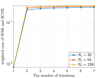
Figure 2: Convergence behaviour of the proposed BCD-based method.

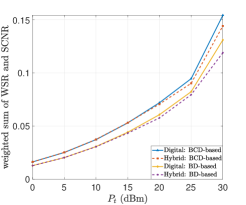
(a) Weighted sum of WSR and SCNR v.s. the transmit power $P_{t}$.

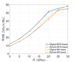
(b) WSR v.s. the transmit power $P_{t}$.

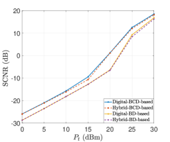
(c) SCNR v.s. the transmit power $P_{t}$.

Figure 3: Weighted sum of WSR and SCNR, WSR, and SCNR v.s. the transmit power $P_{t}$.

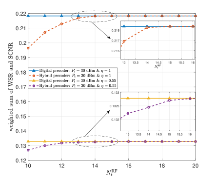
Figure 4: Weighted sum of WSR and SCNR v.s. $N_{t}^{\rm RF}$.

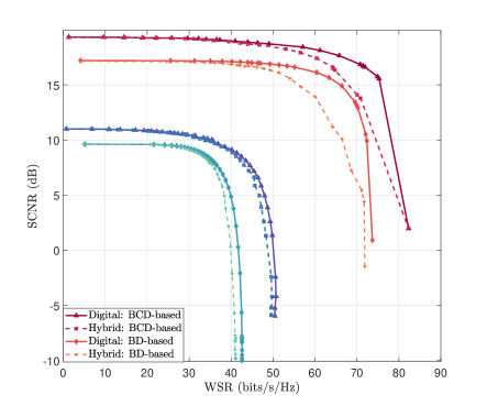
Figure 5: SCNR-WSR performance region by varying $\eta$ in $[0,1]$.

V Simulation Results

In this section, we evaluate the performance of the proposed BCD-based method and the BD-based sub-optimal solution. Unless otherwise stated, the simulation parameters are set as follows. The BS, which is equipped with a uniform linear array (ULA) of $N_{t}=64$ antennas, serves $K=5$ UEs. Each UE is equipped with a ULA of $N_{r}=4$ antennas. The number of data streams is set to $N_{s}=2$. The number of RF chains at the BS and the UE is set to $N_{t}^{\rm RF}=KN_{s}=5\times 2=10$ and $N_{r}^{\rm RF}=N_{s}=2$. The BS and the radar receiver are located at coordinates $[20,30]^{T}$ and $[15,15]^{T}$, respectively. The angular parameters associated with the UEs and the clutter patches are uniformly generated from $[-\pi/2,\pi/2]$. The carrier frequency is set to $28$ GHz. The noise power at each UE and the radar receiver is set to $\sigma^{2}=-90$ dBm.

For communication channels, the complex path gain of the LOS path follows $\beta_{l_{k}}\sim\mathcal{CN}(0,10^{-0.1\kappa})$, where $\kappa=a+10b\log_{10}(d)+\epsilon$, with $d$ being the distance between the BS and the $k$th UE and $\epsilon\in\mathcal{CN}(0,\sigma_{\epsilon}^{2})$ [26]. Here we set $a=61.4$, $b=2$, $\sigma_{\epsilon}=5.8$ dB as suggested in [26]. For non-line-of-sight (NLOS) paths, the complex gain follows a complex Gaussian distribution $\beta_{k,i}\sim\mathcal{CN}(0,10^{-0.1(\kappa+\mu)})$ with $\mu=7$ dB denoting the Rician factor [5]. For sensing response matrices, we set $\sigma_{A}^{2}/\sigma^{2}=20$ dB and $\frac{1}{I}\sum_{i=1}^{I}\sigma_{B_{i}}^{2}/\sigma^{2}=40$ dB for the target and clutter patches, respectively. The weighting coefficient for each UE is set to $w_{k}=1$.

V-A System Performance

Fig. 2 depicts the convergence behaviour of our proposed BCD-based method, where we set the transmit power $P_{t}=30$ dBm and the weighting coefficient $\eta=0.5$. It can be seen that the proposed BCD-based method has a relatively fast convergence rate and attains the maximum objective function value within only $7$ iterations. Moreover, we observe that the convergence rate is independent of the number of antennas at the BS, i.e., $N_{t}$, which is a desirable characteristic for large-scale mmWave systems.

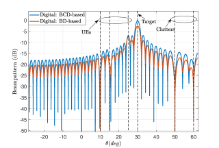
(a) Beam pattern for the first UE.

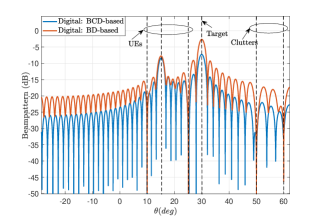
(b) Beam pattern for the second UE.

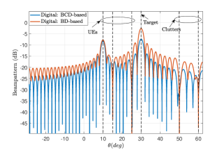
(c) Beam pattern for the third UE.

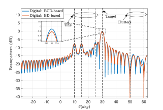
(d) Overall beam pattern.

Figure 6: Transmit beam pattern for different UEs.

In Fig. 3(a), we plot the overall communication-sensing performance as a function of the transmit power $P_{t}$, where the weighting coefficient $\eta$ is set to $0.5$. Also, we depict the WSR and SCNR in Fig. 3(b) and Fig. 3(c), respectively. We see that, as expected, the performance increases as the transmit power $P_{t}$ grows. Also, it is observed that the performance of using the hybrid precoder/combiner is close to the performance attained by fully digital precoder/combiner. Furthermore, the proposed BCD-based method can deliver a better communication/sensing performance than the BD-based solution, and the performance improvement is more pronounced as the transmit power increases.

In Fig. 4, we depict the overall communication-sensing performance of the proposed BCD method versus the number of RF chains $N_{t}^{\rm RF}$, where the transmit power is set to $P_{t}=30$ dBm. To better illustrate the performance, the weighting coefficient is set to $\eta=1$ and $\eta=0.55$, respectively. The total number of resolvable paths at the BS is set to $r=18$, in which the number of clutter patches is set to $I=2$. To illustrate how many RF chains are required, the performance attained by the BCD method with a fully digital precoder is also included for a comparison. We see that when $\eta=1$, which implies only communication performance is concerned, the BCD method with a hybrid precoder achieves the same performance as that of a fully digital precoder using only $N_{t}^{\rm RF}=r-I-1=15$ RF chains. When $\eta=0.55$, the BCD method with a hybrid precoder requires $\tilde{r}=r-I=16$ RF chains to achieve a performance similar to that of a fully digital precoder. This result is attributed to the fact that the radar receive beamforming vector $\boldsymbol{w}$ has effectively eliminate the interference caused by the clutter patches. These results corroborate our theoretical result in Proposition 3 which states that $\tilde{r}$ RF chains are sufficient to achieve the same performance as that of a fully digital precoder.

Fig. 5 illustrates the tradeoff between the communication and sensing performance by varying the weighting coefficient $\eta$ in $[0,1]$, where the transmit power is set to $P_{t}=20$ and $P_{t}=30$ dBm, respectively. From Fig. 5, we see that by choosing a proper weighting coefficient $\eta^{\ast}$, a good balance between the communication and sensing performance can be achieved. Specifically, for such a value of $\eta^{\ast}$, both communication and sensing achieve a decent performance that incurs only a mild performance loss (less than $20\%$) as compared with the performance attained by optimizing exclusively for a single task. Also, a further increase (resp. decrease) of $\eta^{\ast}$ only leads to a small improvement in communication (resp. sensing) performance, but results in a substantial sensing (resp. communication) performance degradation.

V-B Beam Pattern Analysis

To gain insight into the optimized precoder, we examine their transmit beam patterns. In our simulations, we set $\eta=0.5$, $K=3$ and $N_{s}=1$. For simplicity of illustration, the directions of UEs, target and the clutter patches are fixed as $\{10^{\circ},15^{\circ},25^{\circ}\}$, $30^{\circ}$, and $\{50^{\circ},60^{\circ}\}$, respectively. Fig.6(a)-Fig.6(c) depict the beam pattern for each UE, in which the beam pattern for the $k$th UE is defined as $P_{k}(\theta)=\|\boldsymbol{a}_{t}^{H}(\phi_{0})\boldsymbol{F}_{k}\|^{2}$. The transmit power is set to $P_{t}=30$ dBm.

It can be observed in Fig. 6 that for both methods, the optimized radiation pattern forms directional beams towards the target and the served user, and creates nulls in directions pointing to other users as well as the clutter patches. Such a beam pattern can effectively increase the desired communication/radar signal while suppressing interference caused by other users and clutter patches, which is beneficial for improving both sensing and communication performance. We also observe that, despite similar beam patterns, these two methods are slightly different in their power allocation strategies. For the BCD-based method, it tends to allocate more power to the user that is near to the target. Apparently, assigning more power to this user not only helps increase the communication performance, but also improve the sensing accuracy. In contrast, the BD-based analytical solution tends to allocate nearly the same power to each UE. This phenomenon is consistent with the results reported in Proposition 4.

VI Conclusion

In this paper, we studied the problem of joint transceiver design for mmWave/THz ISAC systems. Such a problem was formulated into a non-convex optimization problem whose objective is to maximize the sum of all communication users’ rates and the radar’s received SCNR. By exploring the low-dimensional subspace property of the optimal precoder, we developed a computationally efficient BCD-based algorithm for joint transceiver design. In addition, by generalizing the BD idea to the ISAC system, we proposed an analytical solution to the joint transceiver design problem. Simulation results were provided to illustrate the effectiveness of the proposed methods. Specifically, we showed that by choosing a proper weighting coefficient, the communication and sensing performance can be well balanced, with the performance of each task incurring only a mild performance degradation as compared with the performance attained by optimizing exclusively for a single task.

Appendix A Proof of Proposition 1

$$\sum_{k=1}^{K}\sum_{i=1}^{K}\rho_{c}\alpha_{k}(\boldsymbol{F}_{i}^{\star})^{H}\boldsymbol{H}_{k}^{H}\boldsymbol{W}_{k}\bigg{(}\sum_{j=1}^{K}\boldsymbol{W}_{k}^{H}\boldsymbol{H}_{k}\boldsymbol{F}_{j}^{\star}(\boldsymbol{F}_{j}^{\star})^{H}\boldsymbol{H}_{k}^{H}\boldsymbol{W}_{k}+\sigma_{k}^{2}\boldsymbol{W}_{k}^{H}\boldsymbol{W}_{k}\bigg{)}^{-1}\boldsymbol{W}_{k}^{H}\boldsymbol{H}_{k}\boldsymbol{F}_{i}^{\star}+\frac{\rho_{s}}{f_{2}^{2}}\sum_{i=1}^{K}f_{2}{\rm tr}\left((\boldsymbol{F}_{i}^{\star})^{H}\boldsymbol{A}^{H}\boldsymbol{w}\boldsymbol{w}^{H}\boldsymbol{A}\boldsymbol{F}_{i}^{\star}\right)$$

$$= \sum_{k=1}^{K}\sum_{i\neq k}^{K}\rho_{c}\alpha_{k}(\boldsymbol{F}_{i}^{\star})^{H}\boldsymbol{H}_{k}^{H}\boldsymbol{W}_{k}\bigg{(}\sum_{j\neq k}^{K}\boldsymbol{W}_{k}^{H}\boldsymbol{H}_{k}\boldsymbol{F}_{j}^{\star}(\boldsymbol{F}_{j}^{\star})^{H}\boldsymbol{H}_{k}^{H}\boldsymbol{W}_{k}+\sigma_{k}^{2}\boldsymbol{W}_{k}^{H}\boldsymbol{W}_{k}\bigg{)}^{-1}\boldsymbol{W}_{k}^{H}\boldsymbol{H}_{k}\boldsymbol{F}_{i}^{\star}$$

$$+\frac{\rho_{s}}{f_{2}^{2}}\sum_{i=1}^{K}f_{1,i}{\rm tr}\left((\boldsymbol{F}_{i}^{\star})^{H}\sum_{m=1}^{I}\boldsymbol{B}_{m}^{H}\boldsymbol{w}\boldsymbol{w}^{H}\boldsymbol{B}_{m}\boldsymbol{F}_{i}^{\star}\right)$$ (77)

$$\sum_{k=1}^{K}\rho_{c}w_{k}\sigma_{k}^{2}{\rm tr}\bigg{(}(\boldsymbol{W}_{k}^{H}\boldsymbol{W}_{k})^{-1}\big{(}\sum_{j=1}^{K}\boldsymbol{W}_{k}^{H}\boldsymbol{H}_{k}\boldsymbol{F}_{j}^{\star}(\boldsymbol{F}_{j}^{\star})^{H}\boldsymbol{H}_{k}^{H}\boldsymbol{W}_{k}+\sigma_{k}^{2}\boldsymbol{W}_{k}^{H}\boldsymbol{W}_{k}\big{)}^{-1}\bigg{)}+\frac{\rho_{s}}{f_{2}^{2}}\sum_{i=1}^{K}f_{1,i}\sum_{m=1}^{M}{\rm tr}\left((\boldsymbol{F}_{i}^{\star})^{H}\boldsymbol{B}_{m}^{H}\boldsymbol{w}\boldsymbol{w}^{H}\boldsymbol{B}_{m}\boldsymbol{F}_{i}^{\star}\right)$$

$$= \sum_{k=1}^{K}\rho_{c}w_{k}\sigma_{k}^{2}{\rm tr}\bigg{(}(\boldsymbol{W}_{k}^{H}\boldsymbol{W}_{k})^{-1}\big{(}\sum_{j\neq k}^{K}\boldsymbol{W}_{k}^{H}\boldsymbol{H}_{k}\boldsymbol{F}_{j}^{\star}(\boldsymbol{F}_{j}^{\star})^{H}\boldsymbol{H}_{k}^{H}\boldsymbol{W}_{k}+\sigma_{k}^{2}\boldsymbol{W}_{k}^{H}\boldsymbol{W}_{k}\big{)}^{-1}\bigg{)}+\frac{\rho_{s}}{f_{2}^{2}}\sum_{i=1}^{K}f_{2}{\rm tr}\left((\boldsymbol{F}_{i}^{\star})^{H}\boldsymbol{A}^{H}\boldsymbol{w}\boldsymbol{w}^{H}\boldsymbol{A}\boldsymbol{F}_{i}^{\star}\right)$$ (78)

To demonstrate the low-dimensional subspace property, we first introduce the definition of trivial points and then analyze the KKT conditions of problem (18). Specifically, if a point $\{\boldsymbol{F}_{k}\}_{k=1}^{K}$ satisfying $\boldsymbol{H}_{k}\boldsymbol{F}_{k}=\boldsymbol{0}$ and $\boldsymbol{A}\boldsymbol{F}_{k}=\boldsymbol{0}$, which results in a zero WSR and a zero SCNR, we say it is a trivial point of problem (18). Intuitively, any effective optimized solution to problem (18) should be a non-trivial KKT point. Then, we have the following proposition regarding the dual variable $\lambda^{\star}$.

Proposition 5

For any non-trivial KKT point of problem (18), the dual variable $\lambda^{\star}$ associated with the transmit power constraint must be positive, i.e., $\lambda^{\star}>0$.

Proof:

Denote $\{\boldsymbol{F}_{k}^{\star}\}_{k=1}^{K}$ as the KKT point of the problem (18), which satisfies

$$\rho_{c}w_{k}\nabla_{\boldsymbol{F}_{k}^{\star}}R_{k}(\boldsymbol{F}^{\star})+\rho_{c}\sum_{i\neq k}^{K}w_{i}\nabla_{\boldsymbol{F}_{k}^{\star}}R_{i}(\boldsymbol{F}^{\star})$$

$$+\rho_{s}\nabla_{\boldsymbol{F}_{k}^{\star}}\text{SCNR}(\boldsymbol{F}^{\star})-\lambda^{\star}\boldsymbol{F}_{k}^{\star}=\boldsymbol{0},\forall k,$$ (69)

$$\left(\sum_{k=1}^{K}\operatorname{Tr}\left(\boldsymbol{F}_{k}^{\star}\left(\boldsymbol{F}_{k}^{\star}\right)^{H}\right)-P_{t}\right)\cdot\lambda^{\star}=0,$$ (70)

$$\sum_{k=1}^{K}\operatorname{Tr}\left(\boldsymbol{F}_{k}^{\star}\left(\boldsymbol{F}_{k}^{\star}\right)^{H}\right)\leq P_{\max},$$ (71)

$$\lambda^{\star}\geq 0,$$ (72)

where $R_{k}(\boldsymbol{F}^{\star})$ and $\text{SCNR}(\boldsymbol{F}^{\star})$ are defined in (5) and (12) in terms of $\boldsymbol{F}^{\star}=[\boldsymbol{F}_{1}^{\star}\phantom{0}\ldots\phantom{0}\boldsymbol{F}_{K}^{\star}]\in\mathbb{C}^{N_{t}\times KN_{s}}$, respectively.

We prove $\lambda^{\star}>0$ by contradiction. We first assume $\lambda^{\star}=0$. Note that the gradient of $\nabla_{\boldsymbol{F}_{k}}R_{k}(\boldsymbol{F}^{\star})$, $\nabla_{\boldsymbol{F}_{k}}R_{i}(\boldsymbol{F}^{\star})$, and $\nabla_{\boldsymbol{F}_{k}^{\star}}\text{SCNR}(\boldsymbol{F}^{\star})$ can be respectively calculated as

$$\nabla_{\boldsymbol{F}_{k}^{\star}}R_{k}(\boldsymbol{F}^{\star})= \boldsymbol{H}_{k}^{H}\boldsymbol{W}_{k}\boldsymbol{Z}_{k}^{-1}\boldsymbol{W}_{k}^{H}\boldsymbol{H}_{k}\boldsymbol{F}_{k}^{\star},$$ (73)

$$\nabla_{\boldsymbol{F}_{k}^{\star}}R_{i}(\boldsymbol{F}^{\star})= \boldsymbol{H}_{i}^{H}\boldsymbol{W}_{i}(\boldsymbol{Z}_{i}^{-1}-\tilde{\boldsymbol{Z}}_{i}^{-1})\boldsymbol{W}_{i}^{H}\boldsymbol{H}_{i}\boldsymbol{F}_{k}^{\star},$$ (74)

$$\nabla_{\boldsymbol{F}_{k}^{\star}}\text{SCNR}(\boldsymbol{F}^{\star})= \frac{1}{f_{2}^{2}}(f_{2}\boldsymbol{A}^{H}\boldsymbol{w}\boldsymbol{w}^{H}\boldsymbol{A}\boldsymbol{F}_{k}^{\star}$$

$$-f_{1,k}\sum_{i=1}^{I}\boldsymbol{B}_{i}^{H}\boldsymbol{w}\boldsymbol{w}^{H}\boldsymbol{B}_{i}\boldsymbol{F}_{k}^{\star}),$$ (75)

where

$$\boldsymbol{Z}_{k}= \sum_{j=1}^{K}\boldsymbol{W}_{k}^{H}\boldsymbol{H}_{k}\boldsymbol{F}_{j}^{\star}(\boldsymbol{F}_{j}^{\star})^{H}\boldsymbol{H}_{k}^{H}\boldsymbol{W}_{k}+\sigma_{k}^{2}\boldsymbol{W}_{k}^{H}\boldsymbol{W}_{k},\forall k,$$

$$\tilde{\boldsymbol{Z}}_{i}= \sum_{j\neq i}^{K}\boldsymbol{W}_{i}^{H}\boldsymbol{H}_{i}\boldsymbol{F}_{j}^{\star}(\boldsymbol{F}_{j}^{\star})^{H}\boldsymbol{H}_{i}^{H}\boldsymbol{W}_{i}+\sigma_{i}^{2}\boldsymbol{W}_{i}^{H}\boldsymbol{W}_{i},\forall i,$$

$f_{1,k}=\boldsymbol{w}^{H}\boldsymbol{A}\boldsymbol{F}_{k}^{\star}(\boldsymbol{F}_{k}^{\star})^{H}\boldsymbol{A}^{H}\boldsymbol{w}$ and $f_{2}=\boldsymbol{w}^{H}(\sum_{i=1}^{I}\boldsymbol{B}_{i}\boldsymbol{F}^{\star}(\boldsymbol{F}^{\star})^{H}\boldsymbol{B}_{i}^{H}+\sigma^{2}\boldsymbol{I})\boldsymbol{w}$. Left-multiplying the first-order optimality condition in (69) by $(\boldsymbol{F}_{k}^{\star})^{H}$, we arrive at

$$\rho_{c}w_{k}(\boldsymbol{F}_{k}^{\star})^{H}\nabla_{\boldsymbol{F}_{k}^{\star}}R_{k}(\boldsymbol{F}^{\star})+\rho_{c}\sum_{i\neq k}^{K}w_{i}(\boldsymbol{F}_{k}^{\star})^{H}\nabla_{\boldsymbol{F}_{k}^{\star}}R_{i}(\boldsymbol{F}^{\star})$$

$$+\rho_{s}(\boldsymbol{F}_{k}^{\star})^{H}\nabla_{\boldsymbol{F}_{k}^{\star}}\text{SCNR}(\boldsymbol{F}^{\star})=\boldsymbol{0}.$$ (76)

Taking summation over all $k=1,2,\ldots,K$ gradients in (76) and re-arranging the terms, we could obtain (A) at the top of this page. Using the identities ${\rm tr}(\boldsymbol{A}\boldsymbol{B})={\rm tr}(\boldsymbol{B}\boldsymbol{A})$ and ${\rm tr}(\boldsymbol{A}(\boldsymbol{A}+\boldsymbol{I})^{-1})={\rm tr}(\boldsymbol{I})-{\rm tr}(\boldsymbol{A}+\boldsymbol{I})^{-1}$, we can further obtain (A).

Comparing each term in the left-hand-side and right-hand-side of (A), it can be seen that the equality holds iff $\boldsymbol{H}_{k}\boldsymbol{F}_{k}^{\star}=\boldsymbol{0},\forall k$ and $\boldsymbol{A}\boldsymbol{F}_{k}^{\star}=\boldsymbol{0},\forall k$, which contradicts the fact that $\boldsymbol{F}_{k}^{\star}$ is a non-trivial point. Therefore, we conclude that for any given non-trivial point, the corresponding dual variable $\lambda^{\star}>0$. Also, the full power property can thus be deduced by checking the slack-complementary condition in (70).

Given $\lambda^{\star}>0$, we then prove that the corresponding $\boldsymbol{F}_{k}^{\star}$ must be a non-trivial point. Similarly, we prove it by contradiction. If $\boldsymbol{H}_{k}\boldsymbol{F}_{k}^{\star}=\boldsymbol{0},\forall k$ and $\boldsymbol{A}\boldsymbol{F}_{k}^{\star}=\boldsymbol{0},\forall k$, the gradients in (73) to (75) are equal to zero. In this case, the first-order optimality condition in (69) reduces to $\lambda^{\star}\boldsymbol{F}_{k}^{\star}=\boldsymbol{0}$, which implies $\boldsymbol{F}_{k}^{\star}=\boldsymbol{0}$. This contradicts (70). Therefore, we can conclude that for a non-trivial point $\{\boldsymbol{F}_{k}^{\star}\}_{k=1}^{K}$, the corresponding dual variable $\lambda^{\star}>0$. ∎

Looking back on (69) and noting $\lambda^{\star}>0$, the precoder $\boldsymbol{F}_{k}^{\star}$ can be represented as

$$\boldsymbol{F}_{k}^{\star}= \frac{1}{\lambda}\bigg{(}\rho_{c}w_{k}\nabla_{\boldsymbol{F}_{k}^{\star}}R_{k}(\boldsymbol{F}^{\star})+\sum_{i\neq k}^{K}\rho_{c}w_{i}\nabla_{\boldsymbol{F}_{k}^{\star}}R_{i}(\boldsymbol{F}^{\star})$$

$$+\rho_{s}\nabla_{\boldsymbol{F}_{k}^{\star}}{\text{SCNR}}(\boldsymbol{F}^{\star})\bigg{)}=\boldsymbol{H}^{H}\boldsymbol{G}_{k}$$ (79)

with

$$\boldsymbol{H}\triangleq[\boldsymbol{H}_{1}^{T}\phantom{0}\ldots\phantom{0}\boldsymbol{H}_{K}^{T}\phantom{0}\boldsymbol{A}^{T}\phantom{0}\boldsymbol{B}_{1}^{T}\phantom{0}\ldots\phantom{0}\boldsymbol{B}_{I}^{T}]^{T}\in\mathbb{C}^{M\times N_{t}},$$

$$\boldsymbol{G}_{k}\in\mathbb{C}^{M\times N_{s}},\quad M=KN_{r}+(I+1)N_{\rm sen},$$

It is seen that $\boldsymbol{F}_{k}^{\star}$ must lie in the range space of $\boldsymbol{H}^{H}$. Let $\boldsymbol{V}\in\mathbb{C}^{N_{t}\times r}$ denote the matrix comprising the steering vectors from the BS to all $K$ UEs, the target and all clutters with $r=\sum_{k=1}^{K}L_{k}+I+1$, it is easy to verify that $\boldsymbol{V}$ and $\boldsymbol{H}^{H}$ have the same range space. In other words, the digital precoder $\boldsymbol{F}_{k}^{\star},\forall k$ can be represented by

$$\boldsymbol{F}_{k}^{\star}=\boldsymbol{V}\boldsymbol{X}_{k},$$ (80)

This completes the proof.

Appendix B Proof of Proposition 2

Firstly, it is easy to see that $(\{\boldsymbol{W}_{k}^{\rm opt_{2}},\alpha\boldsymbol{X}_{k}^{\rm opt_{2}}\}_{k=1}^{K},\boldsymbol{w}^{\rm opt_{2}})$ satisfies the transmit power constraint in (22), which shows it is a feasible solution of (22). Next, we show that $(\{\boldsymbol{W}_{k}^{\rm opt_{2}},\alpha\boldsymbol{X}_{k}^{\rm opt_{2}}\}_{k=1}^{K},\boldsymbol{w}^{\rm opt_{2}})$ attains the maximum objective function value in (22). Substituting $(\{\boldsymbol{W}_{k}^{\rm opt_{2}},\alpha\boldsymbol{X}_{k}^{\rm opt_{2}}\}_{k=1}^{K},\boldsymbol{w}^{\rm opt_{2}})$ into the objective function of (22), we arrive at

$$\rho_{c}R(\alpha\boldsymbol{X}_{k}^{\rm opt_{2}},\boldsymbol{W}_{k}^{\rm opt_{2}})+\rho_{s}\text{SCNR}(\boldsymbol{w}^{\rm opt_{2}},\alpha\boldsymbol{X}_{k}^{\rm opt_{2}}),$$

$$= \rho_{c}\bar{R}(\boldsymbol{X}_{k}^{\rm opt_{2}},\boldsymbol{W}_{k}^{\rm opt_{2}})+\rho_{s}\overline{\text{SCNR}}(\boldsymbol{w}^{\rm opt_{2}},\boldsymbol{X}_{k}^{\rm opt_{2}}),$$

$$\geq \rho_{c}\bar{R}(\boldsymbol{X}_{k},\boldsymbol{W}_{k})+\rho_{s}\overline{\text{SCNR}}(\boldsymbol{w},\boldsymbol{X}_{k}),$$

$$\stackrel{{\scriptstyle(a)}}{{=}} \rho_{c}{R}(\tilde{\alpha}\boldsymbol{X}_{k},\boldsymbol{W}_{k})+\rho_{s}{\text{SCNR}}(\boldsymbol{w},\tilde{\alpha}\boldsymbol{X}_{k}),$$ (81)

where $\tilde{\alpha}$ is a scaling factor to satisfy the transmit power constraint and is defined as

$$\tilde{\alpha}=\sqrt{\frac{P_{t}}{\sum_{k=1}^{K}{\rm tr}(\tilde{\boldsymbol{H}}\boldsymbol{X}_{k}(\boldsymbol{X}_{k}^{H})}}.$$ (82)

Hence, the point $(\{\boldsymbol{W}_{k}^{\rm opt_{2}},\alpha\boldsymbol{X}_{k}^{\rm opt_{2}}\}_{k=1}^{K},\boldsymbol{w}^{\rm opt_{2}})$ is the optimal solution to (22). This completes the proof.

References

• [1] Z. Chen, C. Han, Y. Wu, L. Li, C. Huang, Z. Zhang, G. Wang, and W. Tong, “Terahertz Wireless Communications for 2030 and Beyond: A Cutting-Edge Frontier,” IEEE Commun. Mag., vol. 59, no. 11, pp. 66–72, Nov. 2021.
• [2] J. Tan and L. Dai, “THz Precoding for 6G: Challenges, Solutions, and Opportunities,” IEEE Wireless Commun., pp. 1–8, 2022.
• [3] A. Liu, Z. Huang, M. Li, Y. Wan, W. Li, T. X. Han, C. Liu, R. Du, D. K. P. Tan, J. Lu, Y. Shen, F. Colone, and K. Chetty, “A Survey on Fundamental Limits of Integrated Sensing and Communication,” IEEE Commun. Surv. Tutorials, vol. 24, no. 2, pp. 994–1034, 2022.
• [4] F. Liu, C. Masouros, and Y. C. Eldar, Eds., Integrated Sensing and Communications.   Singapore: Springer Nature Singapore, 2023.
• [5] L. Xie, P. Wang, S. Song, and K. B. Letaief, “Perceptive Mobile Network With Distributed Target Monitoring Terminals: Leaking Communication Energy for Sensing,” IEEE Trans. Wireless Commun., vol. 21, no. 12, pp. 10 193–10 207, Dec. 2022.
• [6] P. Wang, J. Fang, L. Dai, and H. Li, “Joint transceiver and large intelligent surface design for massive MIMO mmwave systems,” IEEE Trans. Wireless Commun., vol. 20, no. 2, pp. 1052–1064, Feb. 2021.
• [7] A. Ghosh, T. A. Thomas, M. C. Cudak, R. Ratasuk, P. Moorut, F. W. Vook, T. S. Rappaport, G. R. MacCartney, S. Sun, and S. Nie, “Millimeter-wave enhanced local area systems: a high-data-rate approach for future wireless networks,” IEEE J. Sel. Areas Commun., vol. 32, no. 6, pp. 1152–1163, Jun. 2014.
• [8] S. Rangan, T. S. Rappaport, and E. Erkip, “Millimeter-wave cellular wireless networks: Potentials and challenges,” Proc. IEEE, vol. 102, no. 3, pp. 366–385, Mar. 2014.
• [9] A. Adhikary, E. Al Safadi, M. K. Samimi, R. Wang, G. Caire, T. S. Rappaport, and A. F. Molisch, “Joint spatial division and multiplexing for mm-wave channels,” IEEE J. Sel. Areas Commun., vol. 32, no. 6, pp. 1239–1255, June 2014.
• [10] C. Qi, W. Ci, J. Zhang, and X. You, “Hybrid Beamforming for Millimeter Wave MIMO Integrated Sensing and Communications,” IEEE Commun. Lett., vol. 26, no. 5, pp. 1136–1140, May 2022.
• [11] Z. Cheng and B. Liao, “QoS-Aware Hybrid Beamforming and DOA Estimation in Multi-Carrier Dual-Function Radar-Communication Systems,” IEEE J. Sel. Areas Commun., vol. 40, no. 6, pp. 1890–1905, June 2022.
• [12] X. Wang, Z. Fei, J. A. Zhang, and J. Xu, “Partially-Connected Hybrid Beamforming Design for Integrated Sensing and Communication Systems,” IEEE Trans. Commun., vol. 70, no. 10, pp. 6648–6660, Oct. 2022.
• [13] C. B. Barneto, T. Riihonen, S. D. Liyanaarachchi, M. Heino, N. Gonzalez-Prelcic, and M. Valkama, “Beamformer Design and Optimization for Joint Communication and Full-Duplex Sensing at mm-Waves,” IEEE Trans. Commun., vol. 70, no. 12, pp. 8298–8312, Dec. 2022.
• [14] Z. Cheng, L. Wu, B. Wang, M. R. B. Shankar, and B. Ottersten, “Double-Phase-Shifter Based Hybrid Beamforming for mmWave DFRC in the Presence of Extended Target and Clutters,” IEEE Trans. Wireless Commun., vol. 22, no. 6, pp. 3671–3686, June 2023.
• [15] Z. Cheng, Z. He, and B. Liao, “Hybrid Beamforming for Multi-Carrier Dual-Function Radar-Communication System,” IEEE Trans. Cogn. Commun. Netw., vol. 7, no. 3, pp. 1002–1015, Sept. 2021.
• [16] F. Liu and C. Masouros, “Hybrid Beamforming with Sub-arrayed MIMO Radar: Enabling Joint Sensing and Communication at mmWave Band,” in Proc. IEEE Int. Conf. Acoustics, Speech. Signal Process., Brighton, United Kingdom, May 2019, pp. 7770–7774.
• [17] A. M. Elbir, K. V. Mishra, and S. Chatzinotas, “Terahertz-Band Joint Ultra-Massive MIMO Radar-Communications: Model-Based and Model-Free Hybrid Beamforming,” IEEE J. Sel. Top. Signal Process., vol. 15, no. 6, pp. 1468–1483, Nov. 2021.
• [18] M. A. Islam, G. C. Alexandropoulos, and B. Smida, “Integrated Sensing and Communication with Millimeter Wave Full Duplex Hybrid Beamforming,” in Proc. IEEE Int. Conf. Commun., Seoul, Korea, May 2022, pp. 4673–4678.
• [19] Z. Cheng, Z. He, and B. Liao, “Hybrid Beamforming Design for OFDM Dual-Function Radar-Communication System,” IEEE J. Sel. Top. Signal Process., vol. 15, no. 6, pp. 1455–1467, Nov. 2021.
• [20] L. Chen, Z. Wang, Y. Du, Y. Chen, and F. R. Yu, “Generalized transceiver beamforming for DFRC with MIMO radar and MU-MIMO communication,” IEEE J. Sel. Areas Commun., vol. 40, no. 6, pp. 1795–1808, 2022.
• [21] S. M. Karbasi, A. Aubry, V. Carotenuto, M. M. Naghsh, and M. H. Bastani, “Knowledge-based design of space–time transmit code and receive filter for a multiple-input–multiple-output radar in signal-dependent interference,” IET Radar, Sonar & Navigation, vol. 9, no. 8, pp. 1124–1135, 2015.
• [22] X. Zhao, S. Lu, Q. Shi, and Z.-Q. Luo, “Rethinking WMMSE: Can Its Complexity Scale Linearly With the Number of BS Antennas?” IEEE Trans. Signal Process., vol. 71, pp. 433–446, 2023.
• [23] K. Shen and W. Yu, “Fractional programming for communication systems—part I: Power control and beamforming,” IEEE Trans. Signal Process., vol. 66, no. 10, pp. 2616–2630, 2018.
• [24] H. Kasai, “Fast optimization algorithm on complex oblique manifold for hybrid precoding in millimeter wave MIMO systems,” in Proc. IEEE Global Conf. Signal Info. Process. (GlobalSIP), 2018, pp. 1266–1270.
• [25] D. Tse and P. Viswanath, Fundamentals of wireless communication.   Cambridge university press, 2005.
• [26] S. Sun, T. S. Rappaport, M. Shafi, P. Tang, J. Zhang, and P. J. Smith, “Propagation models and performance evaluation for 5G millimeter-wave bands,” IEEE Trans. Veh. Technol., vol. 67, no. 9, pp. 8422–8439, Sep. 2018.