From Sparse to Dense Functional Data: Phase Transitions from a Simultaneous Inference Perspective

Abstract

We aim to develop simultaneous inference tools for the mean function of functional data from sparse to dense. First, we derive a unified Gaussian approximation to construct simultaneous confidence bands of mean functions based on the B-spline estimator. Then, we investigate the conditions of phase transitions by decomposing the asymptotic variance of the approximated Gaussian process. As an extension, we also consider the orthogonal series estimator and show the corresponding conditions of phase transitions. Extensive simulation results strongly corroborate the theoretical results, and also illustrate the variation of the asymptotic distribution via the asymptotic variance decomposition we obtain. The developed method is further applied to body fat data and traffic data.

Keywords: Phase transitions, Simiultaneous confidence band, Nonparamteric smoothing, Uniform convergence.

1 Introduction

Over the past two decades, functional data analysis has evolved significantly, gaining prominence in diverse fields such as environmental science, industry, and neuroscience. Key resources for foundational concepts in this area include [4], [17], and [21].

Central to functional data analysis is the nonparametric estimation of mean and covariance functions from discretely sampled curves with noise. These estimations are crucial not just as standalone analysis, but also as key components in dimension reduction and further modeling of functional data. This includes applications in functional principal component analysis; see [35], [29], and [6], functional linear regression; see [36], and change point analysis; see [3].

In standard functional data scenarios, we typically encounter $n$ random curves, each representing a subject, with measurement errors at $N_{i}$ random time points for the $i$-th subject. The sampling frequency, denoted as $N_{i}$, plays a pivotal role in the selection of appropriate estimation procedures. Research in this area generally falls into two primary categories: sparse and dense functional data. For sparse functional data, marked by boundedness of $N_{i}$, one often pools data across subjects to gain efficiency, as discussed in [35] and [29], since pre-smoothing is not feasible. On the other hand, for dense functional data, characterized by $N_{i}$ significantly surpassing a certain threshold relative to $n$, one typically adopts nonparametric smoothing for each subject’s data to reduce noise and reconstruct individual curves, as seen in [34] and [28].

Furthermore, [39] performed an in-depth analysis of phase transitions and meticulously investigated convergence rates from sparse to dense functional data, introducing additional subcategories like “semi-dense” and “ultra-dense”. These are based on whether achieving the $\sqrt{n}$ rate and ignoring the asymptotic bias. Also, [33] investigated the estimation of mean derivatives in longitudinal and functional data from sparse to dense. Studies such as [8] and [2] have explored the optimal rates for estimating the mean function in the $\mathcal{L}^{2}$-norm and sup-norm, respectively. More recent work by [37] delved into unified principal component analysis for sparse and dense functional data, especially under spatial dependency conditions. Lastly, [19] achieved significant breakthroughs in non-asymptotic mean and covariance estimation within high-dimensional functional time series. Their contribution is particularly noteworthy for establishing rates for both $\mathcal{L}^{2}$ convergence and uniform convergence, offering powerful tools for convergence analysis when the dimensionality of functional data grows exponentially compared to the sample size.

However, existing asymptotic results mainly address consistency issues, including $\mathcal{L}^{2}$ and uniform convergence, or local asymptotic normality. Simultaneous confidence inference is a vital aspect of functional data analysis. It focuses on the distribution of uniform deviations rather than pointwise asymptotic distributions for constructing confidence intervals. Nonparametric simultaneous confidence bands (SCBs) are essential for simultaneous inference on functions. In dense data contexts, SCBs have been constructed for mean functions; see [11], [28], [24], [23], [26], covariance functions; see [10], [34], [22], and functional principal components; see [6], [5]. [7] introduced a multi-step smoothing method for SCBs of distribution functions of FPC scores. In contrast, the sparse data setting poses challenges for simultaneous inference due to issues like non-tightness of estimators and lack of weak convergence. To the best of our knowledge, [40] is the only work providing the SCBs of mean function on interval $[h,1-h]$ with bandwidth $h$ under sparse sampling, while their method assume the distribution of FPC scores are i.i.d. and follow Gaussian distribution, and the local linear estimator will suffer the boundary problem leading to the SCBs cannot hold on the entire interval $[0,1]$.

This paper introduces a novel methodology for simultaneous inference of the mean function under arbitrary sampling strategies. We propose a B-spline estimator to overcome the shortcomings of kernel smoothing, such as boundary problems and low computational efficiency. Our approach includes a unified Gaussian approximation, facilitating constructing SCBs for mean functions of functional data from sparse to dense. By decomposing asymptotic variance, we observe phase transitions in the approximated Gaussian process. As the number of observation points increases with sample size, we identify three stages of transition, namely “sparse”, “semi-dense”, and “dense”, similar to [39]’s findings. For sparse data, the covariance function of the Gaussian process involves the diagonal of the covariance function of trajectories and the variance function of observation errors. The estimator itself is lack of asymptotic equicontinuity, resulting in no limiting distribution in $C[0,1]$. In dense scenarios, the effect of measurement errors becomes negligible. There exists an intermediate regime between the sparse and dense cases, referred as “semi-dense”, dominated by the contribution of both trajectories and errors, which coincides with results in [2]. Our findings align with those of [39] under specific assumptions, offering more general results relying on the moment of trajectories and the smoothness of the mean function. Furthermore, we establish a sufficient condition for “ultra-dense” sampling, achieving “oracle” efficiency as described in [11], where the estimator is asymptotically equivalent to all the trajectories that can be completely recorded without errors. Additionally, we extend our methodology to general orthogonal series estimators, presenting novel results for simultaneous inference of mean functions from sparse to dense.

The remainder of the paper is structured as follows: Section 2 details the B-spline estimator and its asymptotic properties. Section 3 expands on this framework for orthogonal series estimators. Sections 4 and 5 present implementation details and simulation results, respectively. Application for two real world datasets is illustrated in Section 6, and all proofs of main results are included in supplemental material.

2 Main results

2.1 Notations

Before we describe our methodology, some notations are introduced first. For any vector $\bm{a}=\left(a_{1},\ldots,a_{s}\right)^{\top}\in\mathbb{R}^{s}$, take $\left\|\bm{a}\right\|_{r}=\left(\left|a_{1}\right|^{r}+\ldots+\left|a_{s}\right|^{r}\right)^{1/r}$ for $1\leq r<\infty$, and $\left\|\bm{a}\right\|_{\infty}=\max_{1\leq j\leq s}|a_{j}|$. For any $n\times n$ matrix $\mathbf{A}=(a_{ij})_{i,j=1}^{n}$, denote its $L_{r}$-norm as $\left\|\mathbf{A}\right\|_{r}=\sup_{\left\|x\right\|_{r}=1}\left\|\mathbf{A}x\right\|_{r}$ for $1\leq r\leq\infty$, and particularly $\left\|\mathbf{A}\right\|_{op}=\left\|\mathbf{A}\right\|_{2}$ and $\left\|\mathbf{A}\right\|_{\max}=\max_{1\leq i,j\leq n}|a_{ij}|$. For any function $f(\cdot)$ defined on domain $\mathcal{D}$, denote its sup-norm as $\left\|f\right\|_{\infty}=\sup_{x\in\mathcal{D}}\left|f(x)\right|$, and denote its $\mathcal{L}^{2}$-norm as $\left\|f\right\|_{\mathcal{L}^{2}}=\left\{\int_{\mathcal{D}}f^{2}(x)dx\right\}^{1/2}$. For a real number $\nu\in(0,1]$ and integer $q\in\mathbb{N}$, write $\mathcal{H}_{q,\nu}(\mathcal{D})$ as the space of $(q,\nu)$-Hölder continuous functions on $\mathcal{D}$, that is,

$$\mathcal{H}_{q,\nu}(\mathcal{D})=\left\{h:\mathcal{D}\to\mathbb{R},\leavevmode\nobreak\ \left\|h\right\|_{q,\nu}=\sup_{t,s\in\mathcal{D},t\neq s,\left\|\bm{\alpha}\right\|_{1}=q}\frac{\left|\partial^{\bm{\alpha}}h(t)-\partial^{\bm{\alpha}}h(s)\right|}{\left\|t-s\right\|_{2}^{\nu}}<\infty\right\}.$$

For real numbers $a$ and $b$, $a\wedge b$, $a\vee b$, $\lfloor a\rfloor$ and denote $\min\{a,b\}$, $\max\{a,b\}$ and largest integer that is smaller or equal to $a$, respectively. For two sequences $\{a_{n}\}$ and $\{b_{n}\}$, we write $a_{n}\asymp b_{n}$, $a_{n}\lesssim b_{n}$, $a_{n}\gtrsim b_{n}$, $a_{n}\ll b_{n}$ and $a_{n}\gg b_{n}$ to mean that there exist $c$, $C>0$ such that $0<c\leq|a_{n}/b_{n}|\leq C<\infty$, $a_{n}\leq Cb_{n}$, $b_{n}\leq Ca_{n}$, $a_{n}={\scriptstyle{\mathcal{O}}}(b_{n})$, and $b_{n}={\scriptstyle{\mathcal{O}}}(a_{n})$, respectively. For random variables $X$ and $Y$, we say $X\overset{d}{=}Y$ if they have the same distribution.

2.2 B-spline estimator

For illustration, and without loss of generality, we assume that the domain of the functional data $\eta(x)$ is the unit interval $[0,1]$, which is a square-integrable continuous stochastic process: specifically, $\eta\left(x\right)\in\mathcal{L}^{2}[0,1]$ almost surely, satisfying $\mathbb{E}\int_{0}^{1}\eta^{2}(x)dx<\infty$, with mean function $m(x)$ and covariance function $G(x,x^{\prime})$. According to [21], there exist eigenvalues $\lambda_{1}\geq\lambda_{2}\geq\cdots\geq 0$ with $\sum_{k=1}^{\infty}\lambda_{k}<\infty$, and corresponding eigenfunctions $\left\{\psi_{k}\right\}_{k=1}^{\infty}$ of $G\left(x,x^{\prime}\right)$ being an orthonormal basis of $\mathcal{L}^{2}\left[0,1\right]$, such that $G\left(x,x^{\prime}\right)=\sum_{k=1}^{\infty}\lambda_{k}\psi_{k}(x)\psi_{k}\left(x^{\prime}\right)$, $\int G\left(x,x^{\prime}\right)\psi_{k}\left(x^{\prime}\right)dx^{\prime}=\lambda_{k}\psi_{k}(x)$. The demeaned process $\chi_{i}(x)=\eta_{i}(x)-m(x)$, then allows the well-known Karhunen-Loève representation $\chi_{i}(x)=\sum_{k=1}^{\infty}\xi_{ik}\phi_{k}(x)$, in which the random coefficients $\left\{\xi_{ik}\right\}_{k=1}^{\infty}$, called functional principal component (FPC) scores, are uncorrelated with mean $0$ and variance $1$. The rescaled eigenfunctions $\phi_{k}(x)$, called FPCs, satisfy that $\phi_{k}(x)=\sqrt{\lambda_{k}}\psi_{k}(x)$, for $k\in\mathbb{Z}_{+}$.

Consider the following model:

$$Y_{ij} =\eta_{i}(X_{ij})+\sigma(X_{ij})\epsilon_{ij},\quad 1\leq i\leq n,\,\,1\leq j\leq N_{i}.$$ (2.1)

where covariates $X_{ij}$’s are i.i.d. with density $f(\cdot)$, $\epsilon_{ij}$’s are independent random variables with $\mathbb{E}\left(\epsilon_{ij}\right)=0$ and ${\rm{Var}}\left(\epsilon_{ij}\right)=1$, and $\sigma(\cdot)$ is the variance function of measurement errors. According to the Karhunen-Loève representation, one could further rewrite model (2.1) as

$$Y_{ij}=m(X_{ij})+\sum_{k=1}^{\infty}\xi_{ik}\phi_{k}(X_{ij})+\sigma(X_{ij})\epsilon_{ij},\,\,1\leq i\leq n,\,\,1\leq j\leq N_{i},$$ (2.2)

and $\{\xi_{ik}\}_{i=1,k=1}^{n,\infty}$, $\{\epsilon_{ij}\}_{i=1,j=1}^{n,N_{i}}$ and $\{X_{ij}\}_{i=1,j=1}^{n,N_{i}}$ are mutually independent.

We first consider a B-spline approach to estimate and conduct simultaneous inference for the mean function $m(x)$. To describe the spline functions, let $\{t_{l}\}_{l=0}^{J_{n}+1}$ be a sequence of equally-spaced points, where $t_{l}=l/(J_{n}+1)$ for $0\leq l\leq J_{n}+1$, which divide $[0,1]$ into $J_{n}+1$ equal sub-intervals, denoted as $I_{l}=[t_{l},t_{l+1})$ for $l=0,\ldots,J_{n}-1$, and $I_{J_{n}}=[t_{J_{n}},1]$. Let $\mathcal{S}^{p}_{J_{n}}=\mathcal{S}^{p}_{J_{n}}[0,1]$ be the polynomial spline space of order $p$ over $\left\{I_{l}\right\}_{l=0}^{J_{n}}$, consisting of all functions that are $(p-2)$ times continuously differentiable on $[0,1]$ and are polynomials of degree $(p-1)$ within the sub-intervals $I_{l}$, $l=0,\ldots,J_{n}$. With a little abuse of notation, let $\{B_{l,p}(x)\}_{1\leq l\leq J_{n}+p}$ be the $p$-th order B-spline basis functions of $\mathcal{S}_{J_{n}}^{p}$, then $\mathcal{S}_{J_{n}}^{p}=\left\{\sum_{l=1}^{J_{n}+p}\lambda_{l}B_{l,p}(x):\lambda_{l}\in\mathbb{R}\right\}$.

The mean function $m(x)$ can be estimated by solving the following spline regression, defined as:

$$\hat{m}(x)=\mathop{\arg\min}\limits_{g(\cdot)\in\mathcal{S}_{J_{n}}^{p}}\sum_{i=1}^{n}\sum_{j=1}^{N_{i}}\left\{Y_{ij}-g(X_{ij})\right\}^{2}.$$ (2.3)

Denote $\bar{N}=n^{-1}\sum_{i=1}^{n}N_{i}$, and $p$-th order B-spline basis by $\bm{B}(x)=\bm{B}_{J_{n},p}(x)=\left(B_{1,p}(x),\ldots,B_{J_{n}+p,p}(x)\right)^{\top}$ . The solution to (2.3) is $\hat{m}(x)=\bm{B}^{\top}(x)\hat{\bm{\theta}}$, in which

$$\hat{\bm{\theta}}=\hat{\mathbf{V}}^{-1}\left\{\frac{1}{n\bar{N}}\sum_{i=1}^{n}\sum_{j=1}^{N_{i}}\bm{B}(X_{ij})Y_{ij}\right\},\quad\hat{\mathbf{V}}=\frac{1}{n\bar{N}}\sum_{i=1}^{n}\sum_{j=1}^{N_{i}}\bm{B}(X_{ij})\bm{B}^{\top}(X_{ij}).$$

2.3 Strong approximation by Gaussian processes

In this subsection, we investigate asymptotic properties of the B-spline estimator in (2.3). Without loss of generality, we assume that $N_{i}\geq 2$ for convenience to describe and estimate the covariance structure in the following. Some technical assumptions are introduced for theoretical development.

• Assume that $m(\cdot)\in\mathcal{H}_{q,\nu}[0,1]$ for some integer $q>0$ and some positive real number $\nu\in(0,1]$. In the following, denote by $q^{\ast}=q+\nu$.

• The density function $f(\cdot)$ is bounded above and away from zero, i.e., $c_{f}\leq\inf_{x\in[0,1]}f(x)\leq\sup_{x\in[0,1]}f(x)\leq C_{f}$ for some positive constants $c_{f}$ and $C_{f}$.

• The variance function $\sigma(\cdot)$ of measurement error is uniformly bounded, and $\mathbb{E}|\epsilon_{i}|^{r_{1}}<\infty$ for some integer $r_{1}\geq 3$.

• The covariance function $G(\cdot,\cdot)\in\mathcal{H}_{0,\beta}[0,1]^{2}$ for some $\beta\in(0,1]$, $\inf_{x\in[0,1]}\\ G(x,x)\geq c_{G}$ for some positive constant $c_{G}$, and $\sup_{x\in[0,1]}\mathbb{E}|\eta(x)|^{r_{2}}<\infty$ for some integer $r_{2}\geq 3$.

• Suppose that the spline order $p\geq q^{\ast}$. Let $r=\min\{r_{1},r_{2}\}$, When $\bar{N}\lesssim J_{n}$, $J_{n}^{-q^{\ast}-1/2}n^{1/2}\bar{N}^{1/2}\log^{1/2}(n)={\scriptstyle{\mathcal{O}}}(1),$

  $$J_{n}^{3-2/r}n^{-2+2/r}\bar{N}^{-1}\log^{2}(n)\sum_{i=1}^{n}\left(\sum_{s=1}^{r}N_{i}^{s}J_{n}^{-s}\right)^{2/r}={\scriptstyle{\mathcal{O}}}(1).$$

  When $\bar{N}\gg J_{n}$, $J_{n}^{-q^{\ast}}n^{1/2}\log^{1/2}(n)={\scriptstyle{\mathcal{O}}}(1),$

  $$J_{n}^{4-2/r}n^{-2+2/r}\bar{N}^{-2}\log^{2}(n)\sum_{i=1}^{n}\left(\sum_{s=1}^{r}N_{i}^{s}J_{n}^{-s}\right)^{2/r}={\scriptstyle{\mathcal{O}}}(1).$$

• Let $r=r_{2}$ in (A5).

These assumptions are rather mild. Assumptions (A1) and (A4) are standard conditions to ensure the smoothness of the mean and covariance function in functional data analysis; see [11], [10], [37] and many others. Assumption (A2) is common in the literature for random design; for example, in [8], [39]. Assumptions (A3) and (A4) include some moment conditions on process $\eta_{i}(\cdot)$ and stochastic error $\epsilon_{ij}$. Similar moment conditions are also adopted in [39], [37] and [19]. The range of parameters specified in Assumptions (A1), (A3) and (A4) is given in Assumption (A5). It is worth noting that we do not impose the independence assumption or Gaussian assumption of FPC scores $\xi_{ik}$’s over $k$ or smoothness of FPCs, compared to that in [11], [10], [28] and [40], respectively.

Define $\mathbf{\Sigma}=\mathbf{\Sigma}_{1}+\mathbf{\Sigma}_{2}$, where

$$\mathbf{\Sigma}_{1}=\mathbf{V}^{-1}\mathbb{E}\left\{\frac{\sum_{i=1}^{n}N_{i}(N_{i}-1)}{n\bar{N}^{2}}\bm{B}(X)\bm{B}^{\top}(X^{\prime})G(X,X^{\prime})\right\}\mathbf{V}^{-1},$$

$$\mathbf{\Sigma}_{2}=\mathbf{V}^{-1}\mathbb{E}\left\{\frac{1}{\bar{N}}\bm{B}(X)\bm{B}^{\top}(X)\left(G(X,X)+\sigma^{2}(X)\right)\right\}\mathbf{V}^{-1}.$$

Here, $X$ and $X^{\prime}$ are i.i.d. copies of $X_{ij}$, and $\mathbf{V}=\left\{\mathbb{E}B_{l,p}(X)B_{l^{\prime},p}(X)\right\}_{l,l^{\prime}=1}^{J_{n}+p}$ is the theoretical inner product matrix. Define a Gaussian process $\mathcal{G}_{n}(x)$ with mean zero and covariance structure as follows

$${\text{Cov}}\left(\mathcal{G}_{n}(x),\mathcal{G}_{n}(x^{\prime})\right)=\left\|{\mathbf{\Sigma}}^{1/2}\bm{B}(x)\right\|_{2}^{-1}\bm{B}^{\top}(x){\mathbf{\Sigma}}\bm{B}(x^{\prime})\left\|{\mathbf{\Sigma}}^{1/2}\bm{B}(x^{\prime})\right\|_{2}^{-1}.$$

Theorem 1.

Under Assumptions (A1)-(A5), for some Gaussian vector $\bm{Z}_{n}\sim N(\bm{0},\mathbf{I}_{J_{n}+p})$, as $n\to\infty$,

$$\frac{\sqrt{n}\left\{\hat{m}(x)-m(x)\right\}}{\left\|\mathbf{\Sigma}^{1/2}\bm{B}(x)\right\|_{2}}\overset{d}{=}\frac{\bm{B}^{\top}(x)\mathbf{\Sigma}^{1/2}\bm{Z}_{n}}{\left\|\mathbf{\Sigma}^{1/2}\bm{B}(x)\right\|_{2}}+R_{n}(x)\,\,{\text{in}}\,\,C[0,1],$$

where $\sup_{x\in[0,1]}|R_{n}(x)|={\scriptstyle{\mathcal{O}}}_{p}\left(\log^{-1/2}(n)\right)$. We also have that

$$\sup_{t\in\mathbb{R}}\left|\mathbb{P}\left(\sup_{x\in[0,1]}\frac{\sqrt{n}\left|\hat{m}(x)-m(x)\right|}{\left\|{\mathbf{\Sigma}}^{1/2}\bm{B}(x)\right\|_{2}}\leq t\right)-\mathbb{P}\left(\sup_{x\in[0,1]}\left|\mathcal{G}_{n}(x)\right|\leq t\right)\right|\to 0.$$ (2.4)

We emphasize that we do not restrict the relationship between $n$ and $N_{i}$ in Assumptions (A1)-(A5). In other words, $N_{i}$ can be either fixed, or diverge to infinity at any rate of the sample size $n$. Hence, Theorem 1 provides an approximation of the process $\sqrt{n}\left\|{\mathbf{\Sigma}}^{1/2}\bm{B}(x)\right\|_{2}^{-1}\left\{\hat{m}(x)-m(x)\right\}$ by a sequence of zero-mean Gaussian processes $\mathcal{G}_{n}(\cdot)$ under arbitrary sampling schemes, whether sparse or dense. It can also be construed to assert that, in large samples, the distribution of the process $\hat{m}(\cdot)-m(\cdot)$ depends on the distribution of the data only via matrix $\mathbf{\Sigma}$.

We remark that, one might hope to obtain a result of the following form in Theorem 1,

$$\frac{\sqrt{n}\left\{\hat{m}(x)-m(x)\right\}}{\left\|\mathbf{\Sigma}^{1/2}\bm{B}(x)\right\|_{2}}\xrightarrow{d}\mathcal{G}(x)\,\,{\text{in}}\,\,C[0,1].$$ (2.5)

where $\mathcal{G}(\cdot)$ is some fixed zero-mean Gaussian process. However, the left hand side of (2.5) might not be asymptotically equicontinuous, and so it does not have a limiting distribution. A similar phenomenon has also been discussed in [1]. To address this issue, we provide a sufficient condition to ensure that $\sqrt{n}\left\{\hat{m}(\cdot)-m(\cdot)\right\}$ is asymptotically tight in Section 2.4. Besides, it is noted that the constraints on the value of $J_{n}$ in Assumption (A5) become increasingly loose as $r$ increases. This is because the existence of higher-order moments reduces the dimensional restrictions for strong approximation in [30], which aligns with intuition.

When the order of $\bar{N}$ is higher (lower) than the order of $J_{n}$, one could observe that the matrix $\mathbf{\Sigma}_{2}$ converges to $0$ (diverges to infinity) in the spectral norm sense. Therefore, by introducing additional conditions regarding the comparison of orders between $\bar{N}$ and $J_{n}$, we could obtain phase transitions of strong approximation in the following Theorem 2, which shows that the distribution of the process $\hat{m}(\cdot)-m(\cdot)$ asymptotically depends on the distribution of the data only via matrix $\mathbf{\Sigma}_{2}$ in sparse case, and via matrix $\mathbf{\Sigma}_{1}$ in dense case. Further define Gaussian processes $\mathcal{G}_{1n}(x)$, $\mathcal{G}_{2n}(x)$ with mean zero and covariance structure as follows respectively

$${\text{Cov}}\left(\mathcal{G}_{1n}(x),\mathcal{G}_{1n}(x^{\prime})\right)=\left\|{\mathbf{\Sigma}}_{1}^{1/2}\bm{B}(x)\right\|_{2}^{-1}\bm{B}^{\top}(x){\mathbf{\Sigma}}_{1}\bm{B}(x^{\prime})\left\|{\mathbf{\Sigma}}_{1}^{1/2}\bm{B}(x^{\prime})\right\|_{2}^{-1},$$

$${\text{Cov}}\left(\mathcal{G}_{2n}(x),\mathcal{G}_{2n}(x^{\prime})\right)=\left\|{\mathbf{\Sigma}}_{2}^{1/2}\bm{B}(x)\right\|_{2}^{-1}\bm{B}^{\top}(x){\mathbf{\Sigma}}_{2}\bm{B}(x^{\prime})\left\|{\mathbf{\Sigma}}_{2}^{1/2}\bm{B}(x^{\prime})\right\|_{2}^{-1}.$$

Theorem 2.

Suppose that Assumptions (A1)-(A4) hold and let $\bm{Z}_{n}\sim N(\bm{0},\mathbf{I}_{J_{n}+p})$.

• Under Assumption (A5) and further assume that $\sum_{i=1}^{n}N_{i}^{2}=\mathcal{O}\left(n\bar{N}^{2}\right)$, $\bar{N}\ll J_{n}\log^{-2}(n)$, as $n\to\infty$,

  $$\frac{\sqrt{n}\left\{\hat{m}(x)-m(x)\right\}}{\left\|\mathbf{\Sigma}_{2}^{1/2}\bm{B}(x)\right\|_{2}}\overset{d}{=}\frac{\bm{B}^{\top}(x)\mathbf{\Sigma}_{2}^{1/2}\bm{Z}_{n}}{\left\|\mathbf{\Sigma}_{2}^{1/2}\bm{B}(x)\right\|_{2}}+R_{2n}(x)\,\,{\text{in}}\,\,C[0,1],$$

  where $\sup_{x\in[0,1]}|R_{2n}(x)|={\scriptstyle{\mathcal{O}}}_{p}\left(\log^{-1/2}(n)\right)$. Besides, We have that

  $$\sup_{t\in\mathbb{R}}\left|\mathbb{P}\left(\sup_{x\in[0,1]}\frac{\sqrt{n}\left|\hat{m}(x)-m(x)\right|}{\left\|\mathbf{\Sigma}_{2}^{1/2}\bm{B}(x)\right\|_{2}}\leq t\right)-\mathbb{P}\left(\sup_{x\in[0,1]}\left|\mathcal{G}_{2n}(x)\right|\leq t\right)\right|\to 0.$$ (2.6)

• Under Assumptions (A1)-(A4) and (A5’), and assume $\bar{N}\gg J_{n}\log^{2}(n)$, as $n\to\infty$,

  $$\frac{\sqrt{n}\left\{\hat{m}(x)-m(x)\right\}}{\left\|\mathbf{\Sigma}_{1}^{1/2}\bm{B}(x)\right\|_{2}}\overset{d}{=}\frac{\bm{B}^{\top}(x)\mathbf{\Sigma}_{1}^{1/2}\bm{Z}_{n}}{\left\|\mathbf{\Sigma}_{1}^{1/2}\bm{B}(x)\right\|_{2}}+R_{1n}(x)\,\,{\text{in}}\,\,C[0,1],$$

  where $\sup_{x\in[0,1]}|R_{1n}(x)|={\scriptstyle{\mathcal{O}}}_{p}\left(\log^{-1/2}(n)\right)$. Then, We have that

  $$\sup_{t\in\mathbb{R}}\left|\mathbb{P}\left(\sup_{x\in[0,1]}\frac{\sqrt{n}\left|\hat{m}(x)-m(x)\right|}{\left\|\mathbf{\Sigma}_{1}^{1/2}\bm{B}(x)\right\|_{2}}\leq t\right)-\mathbb{P}\left(\sup_{x\in[0,1]}\left|\mathcal{G}_{1n}(x)\right|\leq t\right)\right|\to 0.$$ (2.7)

Recall that [39] establishes the critical boundary between sparse, semi-dense, and dense by comparing the bias and variance term (lower-order, same-order, higher-order), when discussing the phase transition in uniform convergence and local asymptotic normality. Therefore, the key to distinguishing between sparse and dense lies in two factors: whether the bias term is asymptotically negligible and whether the randomness introduced by measurement error affects the asymptotic variance, which involves the relationship among $n$, $\bar{N}$ and the non-parametric smoothing parameter.

In our discussion of phase transitions in simultaneous inference for the mean function, an essential requirement is that the bias term must be asymptotically negligible. If this condition is not met, conducting simultaneous statistical inference becomes challenging. This is because the bias term in the B-spline estimator, or other orthogonal series estimators introduced in Section 3, does not have an explicit form and cannot be consistently estimated. To satisfy this requirement, a lower bound for $J_{n}$ in relation to $n$ and $\bar{N}$ is necessary. We further note that the phase transition in simultaneous inference primarily depends on the behavior of the variance component $\mathbf{\Sigma}_{2}$, which requires comparing the orders of $J_{n}$ and $\bar{N}$. However, in existing literature, phase transition results are usually described in terms of the relationship between $n$ and $\bar{N}$, as it provides a more intuitive understanding. Following this convention, we predetermine the relationship among $J_{n}$, $n$, and $\bar{N}$ and then translate the relationship between $J_{n}$ and $\bar{N}$ into one between $n$ and $\bar{N}$.

To achieve the optimal convergence rate discussed in [8], we set $J_{n}$ close to its lower bound as outlined in Assumption (A5). This allows us to attain the optimal convergence rate, up to a logarithmic term, and establish phase transitions that vary depending on the smoothness of the mean function. Notably, when $q^{\ast}=2$, our findings align with the phase transition of uniform convergence in [39], differing only by a logarithmic term.

COROLLARY 1.

Suppose that Assumptions (A1)-(A4) hold. Further assume that $\sum_{i=1}^{n}N_{i}^{2s/r}=\mathcal{O}\left(n\bar{N}^{2s/r}\right)$ for each $s=1,2,\ldots,r$. For any fixed $b>1/(2q^{\ast})$,

• Under Assumption (A5), when $\bar{N}\ll n^{1/(2q^{\ast})}\log^{b-(2q^{\ast}+1)/q^{\ast}}(n)$, and $J_{n}\asymp(n\bar{N})^{1/(2q^{\ast}+1)}\log^{2bq^{\ast}/(2q^{\ast}+1)}(n)$, (2.6) holds, referred as “sparse”.

• Under Assumption (A5), when $n^{1/(2q^{\ast})}\log^{b-(2q^{\ast}+1)/q^{\ast}}(n)\lesssim\bar{N}\lesssim n^{1/(2q^{\ast})}\\ \log^{b+2}(n)$, and $J_{n}\asymp n^{1/(2q^{\ast})}\log^{b}(n)$, (2.4) holds, referred as “semi-dense”.

• Under Assumption (A5’), when $\bar{N}\gg n^{\frac{1}{2q^{\ast}}}\log^{b+2}n$, $J_{n}\gg n^{\frac{1}{2q^{\ast}}}\log^{\frac{1}{2q^{\ast}}}(n)$, and $J_{n}\ll\bar{N}\log^{-2}(n)$, (2.7) holds, referred as “dense”.

2.4 The oracle property

In the following, we provide a sufficient condition, known as the oracle property, to ensure the tightness of the process on the left side of (2.5). In functional data analysis, we often say an estimator enjoys oracle efficiency when it is asymptotically indistinguishable from the estimator derived from completely observed trajectories up to order $\sqrt{n}$. To investigate the oracle property of the proposed B-spline estimator, we introduce the following assumptions.

• The rescaled FPCs satisfies $\sum_{k=1}^{\infty}\left\|\phi_{k}(x)\right\|_{\infty}<\infty$, $\sum_{k=1}^{\infty}\left\|\phi_{k}(x)\right\|_{0,\varpi}<\infty$ for some small $\varpi\in(0,1]$.

• Suppose that $p\geq q^{\ast}$, $J_{n}^{-q^{\ast}}n^{1/2}={\scriptstyle{\mathcal{O}}}(1)$, $n^{-1}\bar{N}^{-1}J_{n}^{2}\log(n)={\scriptstyle{\mathcal{O}}}(1)$ and $\bar{N}\gg J_{n}\log(n)$.

Assumption (B1) is a common condition; see [11], [34] for instance, ensuring the boundedness and Hölder continuity of FPCs. The range of parameters is involved in Assumption (B2).

Theorem 3.

Under Assumptions (A1)-(A4) and (B1)-(B2), as $n\to\infty$, we have

$$\sup_{x\in[0,1]}\sqrt{n}\left|\hat{m}(x)-\frac{1}{n}\sum_{i=1}^{n}\frac{N_{i}}{\bar{N}}\eta_{i}(x)\right|={\scriptstyle{\mathcal{O}}}_{p}(1).$$

If $r=\lim_{n\to\infty}n^{-1}\bar{N}^{-2}\sum_{i=1}^{n}N_{i}^{2}$ and $\sum_{i=1}^{n}N_{i}^{2+\delta}=\mathcal{O}\left(n\bar{N}^{2+\delta}\right)$ for some small $\delta>0$, we derive that $\sqrt{n}\left(\hat{m}(x)-m(x)\right)\xrightarrow{d}\sqrt{r}\mathcal{G}_{1}(x)$, where $\mathcal{G}_{1}(x)$ is a mean-zero Gaussian process with covariance function ${\text{Cov}}\left(\mathcal{G}_{1}(x),\mathcal{G}_{1}(x^{\prime})\right)=G(x,x^{\prime})$, and the weak convergence is in the topology of $C[0,1]$.

For regular fixed design ($N_{i}\equiv N$ and $X_{ij}=j/N$), one needs $J_{n}^{-q^{\ast}}n^{1/2}={\scriptstyle{\mathcal{O}}}(1)$, and $J_{n}N^{-1}\log(n)={\scriptstyle{\mathcal{O}}}(1)$ to ensure the oracle property holds, as demonstrated in [11]. These conditions match the parameter ranges required in Theorem 3. However, when $J_{n}\gg N$, the design matrix may not be full rank, which could result in the spline regression in (2.3) having no solution. Therefore, discussing the sparse scenario under regular designs is challenging.

To delve deeper into our findings, it’s crucial to integrate the insights from Theorems 1, 2, 3, and Corollary 1. Let’s start by considering two extreme scenarios. In the first case, imagine each curve has only a single observation point, i.e., $N_{i}\equiv 1$. Under these circumstances, our model (2.2) simplifies to

$$Y_{i}=m(X_{i})+\sum_{k=1}^{\infty}\xi_{ik}\phi_{k}(X_{i})+\sigma(X_{i})\epsilon_{i},\quad 1\leq i\leq n,$$

which resembles a nonparametric regression with independent error and the variance function $G(x,x)+\sigma^{2}(x)$. If $\phi_{k}\equiv 0$ for all $k\in\mathbb{N}$, then our proposed SCBs align with the results in [1]. Conversely, in the scenario of complete trajectory collection, i.e., $N_{i}\equiv\infty$, the inference about the mean function essentially applies the Central Limit Theorem in $C[0,1]$.

For sparse cases like those in [40], where $N_{i}$’s are expectation-finite random variables, they constructed SCBs with a rate $\mathcal{O}_{p}((nh/\log h^{-1})^{-1/2})$, with bandwidth $h$. Our SCBs exhibit a similar rate $\mathcal{O}_{p}((n/J_{n}\log n)^{-1/2})$, aligning with [40] due to $J_{n}\asymp h^{-1}$ and Assumption (A5). The intermediate regime “semi-dense”, situated between the sparse and dense scenarios, is characterized by the combined influence of variation of trajectories and errors, aligning with the findings presented in [2]. In semi-dense and dense cases, our convergence rate is $\mathcal{O}_{p}((n/\log n)^{-1/2})$, identical to that in [39]. In the ultra-dense scenario, where our estimator achieves oracle efficiency, the convergence rate of our SCBs is $\mathcal{O}_{p}(n^{-1/2})$, matching the results in [11].

The phase transition we discuss hinges on the trade-off between ${\rm{Var}}(Y_{ij})$ and ${\rm{Cov}}(Y_{ij},Y_{ij^{\prime}})$. This is evident in the relationship between $\Sigma_{1}$ and $\Sigma_{2}$: $\Sigma_{1}\ll\Sigma_{2}$ in sparse cases, $\Sigma_{1}\asymp\Sigma_{2}$ up to a logarithmic term in semi-dense cases, and $\Sigma_{1}\gg\Sigma_{2}$ in dense cases. Figure 1 visually illustrates our developed boundary, providing an intuitive understanding of these concepts.

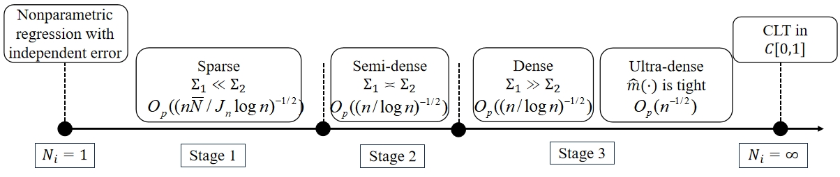
Figure 1: The schema of phase transition phenomena from sparse to dense.

3 Extension to orthogonal series estimators

Let $\{\varphi_{l}(x)\}_{l=1}^{J_{n}}$ be some orthogonal basis functions satisfying $\left\|\varphi_{l}\right\|_{L^{2}}=1$. The mean function $m(x)$ can be also estimated by solving the following orthogonal series regression, defined as:

$$\hat{m}(x)=\mathop{\arg\min}\limits_{\bm{b}\in\mathbb{R}^{J_{n}}}\sum_{i=1}^{n}\sum_{j=1}^{N_{i}}\left\{Y_{ij}-\bm{b}^{\top}\bm{\varphi}(X_{ij})\right\}^{2},$$ (3.1)

in which $\bm{\varphi}(x)=\bm{\varphi}_{n}(x)=\left(\varphi_{1}(x),\ldots,\varphi_{J_{n}}(x)\right)^{\top}$. The solution to (3.1) is $\hat{m}(x)=\bm{\varphi}^{\top}(x)\hat{\bm{\vartheta}}$, where

$$\hat{\bm{\vartheta}}=\hat{\mathbf{Q}}^{-1}\left\{\frac{1}{n\bar{N}}\sum_{i=1}^{n}\sum_{j=1}^{N_{i}}\bm{\varphi}(X_{ij})Y_{ij}\right\},\quad\hat{\mathbf{Q}}=\frac{1}{n\bar{N}}\sum_{i=1}^{n}\sum_{j=1}^{N_{i}}\bm{\varphi}(X_{ij})\bm{\varphi}^{\top}(X_{ij}).$$

The properties of the estimator $\hat{m}(\cdot)$ depend on the characteristics of the adopted basis. To illustrate the approximation power of the basis, which has impact on the convergence rate, we introduce the following two quantities.

$$\kappa^{\bm{\varphi}}_{1,\infty}=\sup_{m\in\mathcal{H}_{q,\nu}[0,1]}\inf_{\bm{b}\in\mathbb{R}^{J_{n}}}\left\|m(\cdot)-\bm{b}^{\top}\bm{\varphi}(\cdot)\right\|_{\infty},$$

$$\kappa^{\bm{\varphi}}_{2,\infty}=\sup_{G\in\mathcal{H}_{s,\beta}[0,1]^{2}}\inf_{\mathbf{A}\in\mathbb{R}^{J_{n}\times J_{n}}}\left\|G(\cdot,\star)-\bm{\varphi}^{\top}(\cdot)\mathbf{A}\bm{\varphi}(\star)\right\|_{\infty}.$$

Another vital feature of the basis associated with uniform asymptotic behaviors of $\hat{m}(\cdot)$ is the linear operators $\Pi^{\bm{\varphi}}_{1}(\cdot)$ and $\Pi^{\bm{\varphi}}_{2}(\cdot)$ defined below,

$$\Pi_{1}^{\bm{\varphi}}(g)=\bm{\varphi}^{\top}(\cdot)\mathbf{Q}^{-1}\mathbb{E}\left\{\bm{\varphi}(X)g(X)\right\},$$

$$\Pi_{2}^{\bm{\varphi}}(h)=\bm{\varphi}^{\top}(\cdot)\mathbf{Q}^{-1}\mathbb{E}\left\{\bm{\varphi}(X)\bm{\varphi}^{\top}(X^{\prime})h(X,X^{\prime})\right\}\mathbf{Q}^{-1}\bm{\varphi}(\star),$$

for any univariate function $g:[0,1]\to\mathbb{R}$ with $\left\|g\right\|_{\infty}<\infty$ and bivariate function $h:[0,1]^{2}\to\mathbb{R}$ with $\left\|h\right\|_{\infty}<\infty$. Define the $L^{\infty}$ operator norm of $\Pi_{1}^{\bm{\varphi}}$ and $\Pi_{2}^{\bm{\varphi}}$ by

$$\left\|\Pi_{1}^{\bm{\varphi}}\right\|_{L^{\infty}}=\sup_{\left\|g\right\|_{\infty}<\infty}\left\|\Pi_{1}^{\bm{\varphi}}(g)\right\|_{\infty}\left\|g\right\|_{\infty}^{-1},\quad\left\|\Pi_{2}^{\bm{\varphi}}\right\|_{L^{\infty}}=\sup_{\left\|h\right\|_{\infty}<\infty}\left\|\Pi_{2}^{\bm{\varphi}}(h)\right\|_{\infty}\left\|h\right\|_{\infty}^{-1}.$$

Below are some examples of orthogonal basis and their relevant features.

Example 1: The Fourier basis functions are defined by $\varphi_{1}(x)=1$, $\varphi_{2k}(x)=\cos(2k\pi x)$ and $\varphi_{2k+1}(x)=\sin(2k\pi x)$ for $k\in\mathbb{Z}_{+}$, forming an orthonormal basis of $\mathcal{L}^{2}[0,1]$. According to discussions in section 3.1 of [1], $\kappa_{1,\infty}^{\varphi}\lesssim J_{n}^{-q-\nu}$ and $\kappa_{2,\infty}^{\varphi}\lesssim J_{n}^{-s-\beta}$ if $m(\cdot)$ and $G(\cdot,\cdot)$ can be extended to periodic functions; see [12] and Corollary 2.4 in Chapter 7 of [16] for reference. From Example 3.7 of [1], $\left\|\Pi_{1}^{\varphi}\right\|_{L^{\infty}}\lesssim\log(J_{n})$ when the density of $X$ is the uniform distribution; see also [41].

Example 2: Cohen-Deubechies-Vial (CDV) wavelet series of order $s_{0}$, described in Example 3.4 of [1], form an orthonormal basis of $\mathcal{L}^{2}[0,1]$. See [14] for more details on CDV wavelet. According to Example 3.9 and Section 3.1 of [1], Example 1 of [32], and Theorem 5.1 of [13], $\kappa_{1,\infty}^{\varphi}\lesssim J_{n}^{-q-\nu}$, $\kappa_{2,\infty}^{\varphi}\lesssim J_{n}^{-s-\beta}$ if the order $s_{0}\geq\max\{q+\nu,s+\beta\}$, and $\left\|\Pi_{1}^{\varphi}\right\|_{L^{\infty}}\lesssim 1$ if the density of $X$ is bounded away from zero and infinity.

Example 3: Legendre polynomial series is the orthonormalizd polynomial series $(1,x,x^{2},\ldots)$ with respect to the Lebesgue measure on $[0,1]$, i.e., $(\varphi_{1},\varphi_{2},\varphi_{3},\ldots)=(1,\sqrt{3}x,\sqrt{5/4}(3x^{2}-1),\ldots)$. From (3.7) in [1] and Theorem 6.2 in Chapter 7 of [16], one obtains $\kappa^{\bm{\varphi}}_{1,\infty}\lesssim J_{n}^{-q-\nu}$ and $\kappa^{\bm{\varphi}}_{2,\infty}\lesssim J_{n}^{-s-\beta}$.

Some technical assumptions are imposed for theoretical development.

• The covariance function $G(\cdot,\cdot)\in\mathcal{H}_{s,\beta}[0,1]^{2}$ for some integar $s\geq 0$ and some $\beta\in(0,1]$.

• Assume that $\left\|\varphi_{l}\right\|_{\infty}\lesssim l^{\rho}$ and $\left\|\varphi_{l}^{\prime}\right\|_{\infty}\lesssim l^{\rho+a}$ for some non-negative real number $\rho,a\geq 0$.

• Assume that $J_{n}^{2\rho+1}n^{-1/2}\bar{N}^{-1/2}\log(n)={\scriptstyle{\mathcal{O}}}(1)$, $\inf_{x\in[0,1]}\left\|\bm{\varphi}(x)\right\|_{2}^{2}\gtrsim J_{n}$, $\kappa^{\bm{\varphi}}_{1,\infty}=\mathcal{O}\left(J_{n}^{-q^{\ast}}\right)$, and $\kappa_{2,\infty}^{\bm{\varphi}}\left\|\Pi_{2}^{\bm{\varphi}}\right\|_{L^{\infty}}={\scriptstyle{\mathcal{O}}}\left(1\right)$. When $\bar{N}\lesssim J_{n}$,

  $$\left\|\Pi_{1}^{\bm{\varphi}}\right\|_{L^{\infty}}J_{n}^{-q^{\ast}-1/2}n^{1/2}\bar{N}^{1/2}\log^{1/2}(n)={\scriptstyle{\mathcal{O}}}(1).$$

  when $\bar{N}\gg J_{n}$, $\left\|\Pi_{1}^{\bm{\varphi}}\right\|_{L^{\infty}}J_{n}^{-q^{\ast}}n^{1/2}\log^{1/2}(n)={\scriptstyle{\mathcal{O}}}(1).$
  For $r=\min\{r_{1},r_{2}\}$, when $\bar{N}\lesssim J_{n}^{2\rho+1}$,

  $$J_{n}^{2\rho+2-2/r}n^{-1+2/r}\bar{N}\log^{2}(n)\left\{\frac{1}{n\bar{N}^{2}}\sum_{i=1}^{n}N_{i}^{2}\right\}={\scriptstyle{\mathcal{O}}}(1).$$

  when $\bar{N}\gg J_{n}^{2\rho+1}$,

  $$J_{n}^{4\rho+3-2/r}n^{-1+2/r}\log^{2}(n)\left\{\frac{1}{n\bar{N}^{2}}\sum_{i=1}^{n}N_{i}^{2}\right\}={\scriptstyle{\mathcal{O}}}(1).$$

• Let $r=r_{2}$ in (C3).

Assumption (C2) is mild and can be verified for many frequently-used basis functions, for instance, $\rho=0,a=1$ for the Fourier basis, and $\rho=1/2,a=2$ for the normalized Legendre basis; see Page 66 of [20], and Pages 17-18 of the Supplement of [15]. We note that the condition $\left\|\varphi_{l}\right\|_{\infty}\lesssim l^{\rho}$ is imposed to derive $\sup_{x\in[0,1]}\left\|\bm{\varphi}(x)\right\|_{2}\lesssim J_{n}^{\rho+1/2}$, and the CDV series satisfies $\sup_{x\in[0,1]}\left\|\bm{\varphi}(x)\right\|_{2}\lesssim J_{n}^{\rho+1/2}$ with $\rho=0$. Besides, As shown in the proofs of Lemmas LABEL:LemmaC1 and LABEL:LemmaC2 in the supplemental material, one could bound $\left\|\Pi_{1}^{\bm{\varphi}}\right\|_{L^{\infty}}\lesssim J_{n}^{\rho+1/2}$ and $\left\|\Pi_{2}^{\bm{\varphi}}\right\|_{L^{\infty}}\lesssim J_{n}^{2\rho+1}$ under Assumption (C2), which are not sharp in many cases, though universally applicable. Thus, it is sufficient to suppose that $\kappa^{\bm{\varphi}}_{2,\infty}=\mathcal{O}\left(J_{n}^{-s-\beta}\right)$ with $s+\beta>2\rho+1$ to ensure $\kappa_{2,\infty}^{\bm{\varphi}}\left\|\Pi_{2}^{\bm{\varphi}}\right\|_{L^{\infty}}={\scriptstyle{\mathcal{O}}}\left(1\right)$. Additionally, elementary calculations show that $\inf_{x\in[0,1]}\left\|\bm{\varphi}(x)\right\|_{2}^{2}\gtrsim J_{n}$ in Assumption (C3) holds at least for the Fourier basis.

Define $\mathbf{\Omega}=\mathbf{\Omega}_{1}+\mathbf{\Omega}_{2}$, where

$$\mathbf{\Omega}_{1}=\mathbf{Q}^{-1}\mathbb{E}\left\{\frac{\sum_{i=1}^{n}N_{i}(N_{i}-1)}{n\bar{N}^{2}}\bm{\varphi}(X)\bm{\varphi}^{\top}(X^{\prime})G(X,X^{\prime})\right\}\mathbf{Q}^{-1},$$

$$\mathbf{\Omega}_{2}=\mathbf{Q}^{-1}\mathbb{E}\left\{\frac{1}{\bar{N}}\bm{\varphi}(X)\bm{\varphi}^{\top}(X)\left(G(X,X)+\sigma^{2}(X)\right)\right\}\mathbf{Q}^{-1}.$$

Here, $X$ and $X^{\prime}$ are i.i.d. copies of $X_{ij}$. Define a Gaussian process $\Xi_{n}(x)$ with mean zero and covariance structure as follows

$${\text{Cov}}\left(\Xi_{n}(x),\Xi_{n}(x^{\prime})\right)=\left\|{\mathbf{\Omega}}^{1/2}\bm{\varphi}(x)\right\|_{2}^{-1}\bm{\varphi}^{\top}(x){\mathbf{\Omega}}\bm{\varphi}(x^{\prime})\left\|{\mathbf{\Omega}}^{1/2}\bm{\varphi}(x^{\prime})\right\|_{2}^{-1}.$$

Further define Gaussian processes $\Xi_{1n}(x)$, $\Xi_{2n}(x)$ with mean zero and covariance structure as follows, respectively

$${\text{Cov}}\left(\Xi_{1n}(x),\Xi_{1n}(x^{\prime})\right)=\left\|{\mathbf{\Omega}}_{1}^{1/2}\bm{\varphi}(x)\right\|_{2}^{-1}\bm{\varphi}^{\top}(x){\mathbf{\Omega}}_{1}\bm{\varphi}(x^{\prime})\left\|{\mathbf{\Omega}}_{1}^{1/2}\bm{\varphi}(x^{\prime})\right\|_{2}^{-1},$$

$${\text{Cov}}\left(\Xi_{2n}(x),\Xi_{2n}(x^{\prime})\right)=\left\|{\mathbf{\Omega}}_{2}^{1/2}\bm{\varphi}(x)\right\|_{2}^{-1}\bm{\varphi}^{\top}(x){\mathbf{\Omega}}_{2}\bm{\varphi}(x^{\prime})\left\|{\mathbf{\Omega}}_{2}^{1/2}\bm{\varphi}(x^{\prime})\right\|_{2}^{-1}.$$

To mimic Theorems 1 and 2, we derive a unified Gaussian approximation and corresponding phase transitions for orthogonal series estimators.

Theorem 4.

Under Assumptions (A1)-(A4), (C1)-(C3), for some $\bm{Z}_{n}\sim N(\bm{0},\mathbf{I}_{J_{n}})$, as $n\to\infty$,

$$\frac{\sqrt{n}\left\{\hat{m}(x)-m(x)\right\}}{\left\|\mathbf{\Omega}^{1/2}\bm{\varphi}(x)\right\|_{2}}\overset{d}{=}\frac{\bm{\varphi}^{\top}(x)\mathbf{\Omega}^{1/2}\bm{Z}_{n}}{\left\|\mathbf{\Omega}^{1/2}\bm{\varphi}(x)\right\|_{2}}+R_{n}^{\dagger}(x)\,\,{\text{in}}\,\,C[0,1],$$

where $\sup_{x\in[0,1]}|R^{\dagger}_{n}(x)|={\scriptstyle{\mathcal{O}}}_{p}\left(\log^{-1/2}(n)\right)$. We also have that

$$\sup_{t\in\mathbb{R}}\left|\mathbb{P}\left(\sup_{x\in[0,1]}\frac{\sqrt{n}\left|\hat{m}(x)-m(x)\right|}{\left\|{\mathbf{\Omega}}^{1/2}\bm{\varphi}(x)\right\|_{2}}\leq t\right)-\mathbb{P}\left(\sup_{x\in[0,1]}\left|\Xi_{n}(x)\right|\leq t\right)\right|\to 0.$$ (3.2)

Theorem 5.

Suppose that Assumptions (A1)-(A4), (C1),(C2) hold and let $\bm{Z}_{n}\sim N(\bm{0},\mathbf{I}_{J_{n}})$.

• Under (C3) and further assume $\sum_{i=1}^{n}N_{i}^{2}=\mathcal{O}\left(n\bar{N}^{2}\right)$ and $\bar{N}\ll\\ J_{n}\log^{-2}(n)$, as $n\to\infty$,

  $$\frac{\sqrt{n}\left\{\hat{m}(x)-m(x)\right\}}{\left\|\mathbf{\Omega}_{2}^{1/2}\bm{\varphi}(x)\right\|_{2}}\overset{d}{=}\frac{\bm{\varphi}^{\top}(x)\mathbf{\Omega}_{2}^{1/2}\bm{Z}_{n}}{\left\|\mathbf{\Omega}_{2}^{1/2}\bm{\varphi}(x)\right\|_{2}}+R_{2n}^{\dagger}(x)\,\,{\text{in}}\,\,C[0,1],$$

  where $\sup_{x\in[0,1]}|R_{2n}^{\dagger}(x)|={\scriptstyle{\mathcal{O}}}_{p}\left(\log^{-1/2}(n)\right)$. We also have that

  $$\sup_{t\in\mathbb{R}}\left|\mathbb{P}\left(\sup_{x\in[0,1]}\frac{\sqrt{n}\left|\hat{m}(x)-m(x)\right|}{\left\|\mathbf{\Omega}_{2}^{1/2}\bm{\varphi}(x)\right\|_{2}}\leq t\right)-\mathbb{P}\left(\sup_{x\in[0,1]}\left|\Xi_{2n}(x)\right|\leq t\right)\right|\to 0.$$ (3.3)

• Under (C3’) and further assume $\bar{N}\gg J_{n}^{2\rho+1}\log^{2}(n)$, as $n\to\infty$,

  $$\frac{\sqrt{n}\left\{\hat{m}(x)-m(x)\right\}}{\left\|\mathbf{\Omega}_{1}^{1/2}\bm{\varphi}(x)\right\|_{2}}\overset{d}{=}\frac{\bm{\varphi}^{\top}(x)\mathbf{\Omega}_{1}^{1/2}\bm{Z}_{n}}{\left\|\mathbf{\Omega}_{1}^{1/2}\bm{\varphi}(x)\right\|_{2}}+R_{1n}^{\dagger}(x)\,\,{\text{in}}\,\,C[0,1],$$

  where $\sup_{x\in[0,1]}|R_{1n}^{\dagger}(x)|={\scriptstyle{\mathcal{O}}}_{p}\left(\log^{-1/2}(n)\right)$. We also have that

  $$\sup_{t\in\mathbb{R}}\left|\mathbb{P}\left(\sup_{x\in[0,1]}\frac{\sqrt{n}\left|\hat{m}(x)-m(x)\right|}{\left\|\mathbf{\Omega}_{1}^{1/2}\bm{\varphi}(x)\right\|_{2}}\leq t\right)-\mathbb{P}\left(\sup_{x\in[0,1]}\left|\Xi_{1n}(x)\right|\leq t\right)\right|\to 0.$$ (3.4)

It is noted that the constraint on the range of parameter $J_{n}$ in assumption (C3) is more stringent than that in (A5). These are due to the local compact support property of B-splines, as well as the appealing properties of uniform bound for the bias terms in B-spline estimators, highlighting their advantages over general orthogonal basis.

Inspired by Theorems 4 and 5, we state the phase transition as follows.

COROLLARY 2.

Suppose that Assumptions (A1)-(A4), (C1)-(C2) hold. Further assume that $\sum_{i=1}^{n}N_{i}^{2}=\mathcal{O}\left(n\bar{N}^{2}\right)$ and $\left\|\Pi_{1}^{\bm{\varphi}}\right\|_{L^{\infty}}=\mathcal{O}\left(\log^{\tau}(n)\right)$ for some $\tau>0$. For any fixed $b>(2\tau+1)/(2q^{\ast})$,

• Under Assumption (C3), when $\bar{N}\ll n^{1/(2q^{\ast})}\log^{b-(2q^{\ast}+1)/q^{\ast}}(n)$, and $J_{n}\asymp\left(n\bar{N}\right)^{1/(2q^{\ast}+1)}\log^{2bq^{\ast}/(2q^{\ast}+1)}(n)$, (3.3) holds, referred as “sparse”.

• Under Assumption (C3), when $n^{1/(2q^{\ast})}\log^{b-(2q^{\ast}+1)/q^{\ast}}(n)\lesssim\bar{N}\lesssim\\ n^{(2\rho+1)/(2q^{\ast})}\log^{(2\rho+1)b+2}(n)$, and $J_{n}\asymp n^{1/(2q^{\ast})}\log^{b}(n)$, (3.2) holds, referred as “semi-dense”.

• Under Assumption (C3’), when $\bar{N}\gg n^{(2\rho+1)/(2q^{\ast})}\log^{(2\rho+1)b+2}(n)$, and $J_{n}\gg n^{1/(2q^{\ast})}\log^{b}(n)$, $J_{n}^{2\rho+1}\log^{2}(n)\ll\bar{N}$, (3.4) holds, referred as “dense”.

4 Implementation

In this section, we focus on the estimation of the covariance structure of the proposed B-spline estimator. Since it is not difficult to extend to that of the orthogonal series estimator developed in Section 3, details are omitted to save space.

Denote by $\hat{U}_{ij}=Y_{ij}-\hat{m}(X_{ij})$. The matrix $\mathbf{\Sigma}$ can be estimated by $\hat{\mathbf{\Sigma}}=\hat{\mathbf{\Sigma}}_{1}+\hat{\mathbf{\Sigma}}_{2}$, where

$$\hat{\mathbf{\Sigma}}_{1}=\hat{\mathbf{V}}^{-1}\left\{\frac{1}{n\bar{N}^{2}}\sum_{i=1}^{n}\sum_{j\neq j^{\prime}}^{N_{i}}\bm{B}(X_{ij})\bm{B}^{\top}(X_{ij^{\prime}})\hat{U}_{ij}\hat{U}_{ij^{\prime}}\right\}\hat{\mathbf{V}}^{-1},$$ (4.1)

$$\hat{\mathbf{\Sigma}}_{2}=\hat{\mathbf{V}}^{-1}\left\{\frac{1}{n\bar{N}^{2}}\sum_{i=1}^{n}\sum_{j=1}^{N_{i}}\bm{B}(X_{ij})\bm{B}^{\top}(X_{ij})\hat{U}_{ij}^{2}\right\}\hat{\mathbf{V}}^{-1}.$$

Compared with the covariance estimation in [35], [11], [10], [39] and many others, we emphasize that the proposed estimator $\hat{\mathbf{\Sigma}}$ of the covariance structure is guaranteed to be positive semi-definite, thus no additional procedures are employed to adjust the estimated covariance structure.

To proceed, it suffices to obtain the quantile of the sup-norm of $\mathcal{G}_{n}(\cdot)$, denote by $Q_{1-\alpha}$, to construct feasible SCB for the mean function from sparse to dense. It would be challenging to directly derive the distribution $\sup_{x\in[0,1]}\left|\mathcal{G}_{n}(x)\right|$ analytically and calculate its quantile $Q_{1-\alpha}$. To obtain the estimated quantile, it is vital to generate Gaussian process, denoted by $\zeta_{n}(\cdot)$, whose covariance structure mimics that of $\mathcal{G}_{n}(\cdot)$ by the plug-in principle. The following describes how to efficiently generate a sequence of random processes $\{\zeta_{b,n}(\cdot)\}_{b=1}^{B}$, which are i.i.d. copies of $\zeta_{n}(\cdot)$. Given the data $\{X_{ij},Y_{ij}\}_{i=1,j=1}^{n,N_{i}}$, one generates i.i.d. $(J_{n}+p)$-dimensional Gaussian random vectors $\{\bm{Z}_{b,n}\}_{b=1}^{B}$ with mean zero and covariance matrix $\hat{\mathbf{\Sigma}}$ and let $\zeta_{b,n}(\cdot)=\left\|\hat{\mathbf{\Sigma}}^{1/2}\bm{B}(\cdot)\right\|_{2}^{-1}\bm{B}^{\top}(\cdot)\bm{Z}_{b,n}$. Thus, we have

$${\text{Cov}}\left(\zeta_{n}(x),\zeta_{n}(x^{\prime})\right)=\left\|\hat{\mathbf{\Sigma}}^{1/2}\bm{B}(x)\right\|_{2}^{-1}\bm{B}^{\top}(x)\hat{\mathbf{\Sigma}}\bm{B}(x^{\prime})\left\|\hat{\mathbf{\Sigma}}^{1/2}\bm{B}(x^{\prime})\right\|_{2}^{-1}.$$

The following theorem shows the uniform consistency of the estimated covariance structure and the asymptotic standard deviation function of process $\sqrt{n}\left\{\hat{m}(\cdot)-m(\cdot)\right\}$.

• The parameters $r_{1},r_{2}\geq 4$ in Assumption (A3), (A4).

Theorem 6.

Assume that $\sum_{i=1}^{n}N_{i}(N_{i}-1)=\mathcal{O}\left(n\bar{N}^{2}\right)$, $\sum_{i=1}^{n}N_{i}(N_{i}-1)^{2}=\mathcal{O}\left(n\bar{N}^{3}\right)$, and $\sum_{i=1}^{n}N_{i}(N_{i}-1)(N_{i}-2)(N_{i}-3)=\mathcal{O}\left(n\bar{N}^{4}\right)$. Under Assumptions (A1)-(A5), (D1) and $n^{-1/2}\bar{N}^{-1/2}J_{n}^{2}\log^{1/2}(n)={\scriptstyle{\mathcal{O}}}(1)$, as $n\to\infty$,

$$\sup_{x,x^{\prime}\in[0,1]}\left|{\text{Cov}}\left(\zeta_{n}(x),\zeta_{n}(x^{\prime})\right)-{\text{Cov}}\left(\mathcal{G}_{n}(x),\mathcal{G}_{n}(x^{\prime})\right)\right|={\scriptstyle{\mathcal{O}}}_{p}\left(1\right),$$

$$\sup_{x\in[0,1]}\left|\left\|\hat{\mathbf{\Sigma}}^{1/2}\bm{B}(x)\right\|_{2}-\left\|\mathbf{\Sigma}^{1/2}\bm{B}(x)\right\|_{2}\right|={\scriptstyle{\mathcal{O}}}_{p}\left(1\right).$$

Denote by $\hat{Q}_{1-\alpha}$ the upper-$\alpha$ quantile of the sup-norm of $\zeta_{n}(\cdot)$. Then, the asymptotically correct SCB of confidence level $1-\alpha$ for the mean function is defined by

$$\left(\hat{m}(x)-\frac{\hat{Q}_{1-\alpha}}{\sqrt{n}}\left\|\hat{\mathbf{\Sigma}}^{1/2}\bm{B}(x)\right\|_{2},\hat{m}(x)+\frac{\hat{Q}_{1-\alpha}}{\sqrt{n}}\left\|\hat{\mathbf{\Sigma}}^{1/2}\bm{B}(x)\right\|_{2}\right),\quad x\in[0,1].$$

5 Numerical simulations

In this section, numerical simulation studies are conducted to assess the finite-sample performance of the proposed SCB via B-splines. The data are generated from model (2.2). A total of four sampling schemes from sparse to dense are taken into consideration. We assume that $N_{i}$ are i.i.d. from a discrete uniform distribution on the set: (1) $\{3,4,5,6\}$, (2) $\{\lfloor 2n^{1/5}\rfloor,\lfloor 2n^{1/5}\rfloor+1,\ldots,\lfloor 4n^{1/5}\rfloor\}$, (3) $\{\lfloor n^{1/2}\rfloor,\lfloor n^{1/2}\rfloor+1,\ldots,\lfloor 2n^{1/2}\rfloor\}$, and (4) $\{\lfloor n/4\rfloor,\lfloor n/4\rfloor+1,\ldots,\lfloor n/2\rfloor\}$.

In each case, we set $m(x)=3/2\sin\{3\pi(x+1/2)\}+2x^{3}$, $\lambda_{k}=2^{1-k}$ for $k=1,\ldots,4$ and $\lambda_{k}=0$ for $k\geq 5$, $\psi_{2k-1}=\sqrt{2}\sin(2k\pi x)$ and $\psi_{2k}=\sqrt{2}\cos(2k\pi x)$ for $k\in\mathbb{Z}_{+}$. Besides, $\{\xi_{tk}\}_{t=1,k=1}^{n,\infty}$ are i.i.d random variables. We consider the variance function $\sigma^{2}(\cdot)$ as in a homoscedastic case with $\sigma(x)=\sigma_{\varepsilon}$ and in a heteroscedastic case with $\sigma(x)=1.2\sigma_{\varepsilon}\left(5-\exp(-x)\right)/\left(5+\exp(-x)\right).$ The noise level is set at $\sigma_{\varepsilon}=0.1$. We also consider different distributions of the FPC scores and the errors, including the standard Normal distribution $N(0,1)$, the Uniform distribution $U(-\sqrt{3},\sqrt{3})$, and the standardized Laplace distribution with density $f(x)=2^{-1/2}\exp(\sqrt{2}|x|)$. The number of sample size $n$ is set at $100$, $200$, and $400$. The empirical replications $B$ in quantile estimation and the Monte Carlo replications are both $500$.

The number of knots $J_{n}$ is a fundamental smoothing parameter and a data-driven method proposed in [25] that minimizes the BIC value corresponding to $J_{n}\in[0.5(n\bar{N})^{1/6},2(n\bar{N})^{1/4}]$ is what we recommend. Note that this specific range satisfies the assumptions and contains enough candidates without increasing too much computational burden. The BIC value is defined as

$$\mathrm{BIC}\left(J_{n}\right)=\log\left[(n\bar{N})^{-1}\sum_{i=1}^{n}\sum_{j=1}^{N_{i}}\left\{Y_{ij}-\widehat{m}_{J_{n}}(X_{ij})\right\}^{2}\right]+\frac{J_{n}\log(n\bar{N})}{n\bar{N}},$$ (5.1)

where $\widehat{m}_{J_{n}}$ is the estimator defined in (2.3) with the number of knots $J_{n}$.

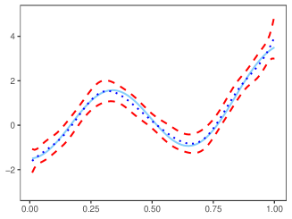
(a) Setting 1

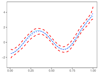
(b) Setting 2

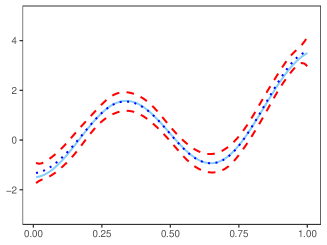
(c) Setting 3

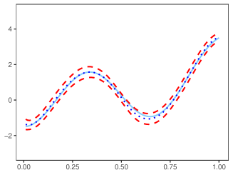
(d) Setting 4

Figure 2: Numerical simulation with $n=200$. Solid line: the true mean function; dotted line: the estimated mean function using cubic B-splines; dashed line: the proposed SCB at the significance level of $95\%$.

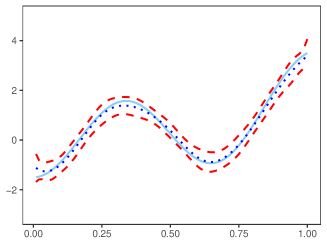
(a) Setting 1

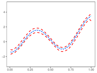
(b) Setting 2

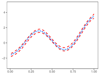
(c) Setting 3

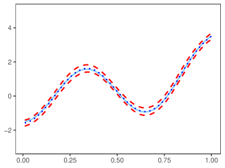
(d) Setting 4

Figure 3: Numerical simulation with $n=400$. Solid line: the true mean function; dotted line: the estimated mean function using cubic B-splines; dashed line: the proposed SCB at the significance level of $95\%$.

For comparison, we also implement the simultaneous inference procedure developed in [11], denoted by CYT in Tables 1-3. To illustrate the asymptotic variance decomposition transitioning from sparse to dense, we also report the values of $\|\hat{\mathbf{\Sigma}}_{1}\|_{\infty}$ and $\|\hat{\mathbf{\Sigma}}_{2}\|_{\infty}$. Tables 1-3 show that in each setting, the empirical coverage rates of the proposed SCBs are close to the nominal confidence level $95\%$. Figures 2 and 3 respectively display the estimated mean functions and corresponding $95\%$ SCBs with $n=200$ and $n=400$ in different settings, which show the true mean function is fully encompassed within the SCBs and the SCBs narrow as $n$ increases. These strongly reveal a positive confirmation of the asymptotic theory. However, it is seen that the method developed in [11] performs well only in the dense scenario with a large sample size, namely experiments with $n=400$ in Setting 4.

Table 1: Empirical coverage rates of $95\%$ SCBs for the mean function $m(x)$ with a sample size of $n=100$.

		Homoscedastic (Heteroscedastic) error
$\xi$	$\epsilon$	Normal	Uniform	Laplace	Normal	Uniform	Laplace
		Setting 1			Setting 2
Normal	New	0.900(0.898)	0.882(0.894)	0.898(0.908)	0.884(0.926)	0.902(0.894)	0.926(0.940)
	CYT	0.240(0.260)	0.208(0.252)	0.260(0.270)	0.386(0.444)	0.406(0.400)	0.444(0.438)
	$\|\hat{\mathbf{\Sigma}}_{1}\|_{\infty}$	10.23(10.49)	10.30(10.25)	10.49(10.21)	7.24(7.25)	7.11(7.09)	7.25(7.07)
	$\|\hat{\mathbf{\Sigma}}_{2}\|_{\infty}$	34.03(35.05)	33.99(33.91)	35.05(33.94)	15.86(16.09)	15.74(15.90)	16.09(15.74)
Uniform	New	0.884(0.864)	0.890(0.884)	0.864(0.886)	0.924(0.900)	0.882(0.900)	0.900(0.914)
	CYT	0.194(0.234)	0.242(0.200)	0.234(0.188)	0.396(0.378)	0.418(0.424)	0.378(0.400)
	$\|\hat{\mathbf{\Sigma}}_{1}\|_{\infty}$	9.24(9.39)	9.32(9.14)	9.39(9.12)	6.63(6.56)	6.72(6.41)	6.56(6.57)
	$\|\hat{\mathbf{\Sigma}}_{2}\|_{\infty}$	33.04(33.27)	33.23(33.32)	33.27(33.23)	15.48(15.47)	15.57(15.47)	15.47(15.57)
Laplace	New	0.898(0.908)	0.888(0.890)	0.908(0.916)	0.912(0.914)	0.910(0.918)	0.914(0.922)
	CYT	0.236(0.206)	0.252(0.246)	0.206(0.250)	0.426(0.450)	0.418(0.448)	0.450(0.442)
	$\|\hat{\mathbf{\Sigma}}_{1}\|_{\infty}$	12.16(12.20)	12.05(12.04)	12.20(12.65)	8.17(8.36)	8.05(7.95)	8.36(8.12)
	$\|\hat{\mathbf{\Sigma}}_{2}\|_{\infty}$	35.50(35.93)	34.53(35.46)	35.93(35.70)	16.47(16.61)	16.24(16.28)	16.61(16.61)
		Setting 3			Setting 4
Normal	New	0.926(0.928)	0.926(0.928)	0.928(0.938)	0.938(0.940)	0.930(0.944)	0.940(0.924)
	CYT	0.534(0.576)	0.564(0.586)	0.576(0.542)	0.778(0.790)	0.770(0.780)	0.790(0.746)
	$\|\hat{\mathbf{\Sigma}}_{1}\|_{\infty}$	6.33(6.22)	6.49(6.36)	6.22(6.19)	5.67(5.65)	5.68(5.62)	5.65(5.67)
	$\|\hat{\mathbf{\Sigma}}_{2}\|_{\infty}$	9.25(9.09)	9.22(9.31)	9.09(9.15)	3.58(3.57)	3.60(3.60)	3.57(3.60)
Uniform	New	0.910(0.914)	0.930(0.890)	0.914(0.906)	0.944(0.942)	0.930(0.934)	0.942(0.918)
	CYT	0.556(0.528)	0.546(0.538)	0.528(0.508)	0.774(0.774)	0.774(0.780)	0.774(0.746)
	$\|\hat{\mathbf{\Sigma}}_{1}\|_{\infty}$	6.04(6.03)	5.90(6.04)	6.03(5.94)	5.48(5.58)	5.54(5.57)	5.58(5.47)
	$\|\hat{\mathbf{\Sigma}}_{2}\|_{\infty}$	9.12(9.10)	9.12(9.11)	9.10(9.03)	3.58(3.55)	3.56(3.57)	3.55(3.55)
Laplace	New	0.894(0.916)	0.934(0.946)	0.916(0.918)	0.940(0.932)	0.922(0.922)	0.932(0.948)
	CYT	0.566(0.574)	0.606(0.592)	0.574(0.562)	0.788(0.768)	0.744(0.782)	0.768(0.800)
	$\|\hat{\mathbf{\Sigma}}_{1}\|_{\infty}$	7.02(7.02)	7.21(7.02)	7.02(7.07)	5.91(5.91)	6.03(5.86)	5.91(5.97)
	$\|\hat{\mathbf{\Sigma}}_{2}\|_{\infty}$	9.39(9.37)	9.36(9.37)	9.37(9.51)	3.69(3.64)	3.67(3.64)	3.64(3.65)

Table 2: Empirical coverage rates of $95\%$ SCBs for the mean function $m(x)$ with a sample size of $n=200$.

		Homoscedastic (Heteroscedastic) error
$\xi$	$\epsilon$	Normal	Uniform	Laplace	Normal	Uniform	Laplace
		Setting 1			Setting 2
Normal	New	0.912(0.924)	0.928(0.924)	0.924(0.942)	0.934(0.916)	0.926(0.916)	0.916(0.940)
	CYT	0.192(0.180)	0.190(0.200)	0.180(0.192)	0.466(0.418)	0.482(0.440)	0.418(0.444)
	$\|\hat{\mathbf{\Sigma}}_{1}\|_{\infty}$	8.47(8.52)	8.47(8.81)	8.52(8.48)	5.26(5.43)	5.37(5.41)	5.43(5.17)
	$\|\hat{\mathbf{\Sigma}}_{2}\|_{\infty}$	36.54(36.52)	36.52(36.96)	36.52(36.40)	13.59(13.55)	13.51(13.52)	13.55(13.49)
Uniform	New	0.908(0.906)	0.902(0.900)	0.906(0.910)	0.914(0.932)	0.924(0.934)	0.932(0.930)
	CYT	0.164(0.170)	0.200(0.182)	0.170(0.168)	0.432(0.456)	0.468(0.470)	0.456(0.480)
	$\|\hat{\mathbf{\Sigma}}_{1}\|_{\infty}$	7.59(7.60)	7.82(7.71)	7.60(7.58)	4.89(4.94)	4.93(4.95)	4.94(5.03)
	$\|\hat{\mathbf{\Sigma}}_{2}\|_{\infty}$	36.21(36.02)	36.11(36.09)	36.02(35.71)	13.45(13.40)	13.49(13.51)	13.40(13.44)
Laplace	New	0.932(0.912)	0.922(0.926)	0.912(0.930)	0.954(0.934)	0.938(0.928)	0.934(0.936)
	CYT	0.210(0.218)	0.212(0.202)	0.218(0.218)	0.496(0.476)	0.484(0.446)	0.476(0.492)
	$\|\hat{\mathbf{\Sigma}}_{1}\|_{\infty}$	10.44(10.37)	10.53(9.86)	10.37(10.48)	6.18(6.08)	6.11(6.17)	6.08(6.02)
	$\|\hat{\mathbf{\Sigma}}_{2}\|_{\infty}$	37.95(38.15)	38.33(37.71)	38.15(38.03)	13.93(13.86)	13.96(13.84)	13.86(13.62)
		Setting 3			Setting 4
Normal	New	0.946(0.920)	0.938(0.944)	0.920(0.906)	0.938(0.958)	0.934(0.950)	0.958(0.942)
	CYT	0.618(0.564)	0.602(0.580)	0.564(0.620)	0.874(0.846)	0.848(0.880)	0.846(0.850)
	$\|\hat{\mathbf{\Sigma}}_{1}\|_{\infty}$	4.73(4.74)	4.76(4.66)	4.74(4.70)	4.19(4.20)	4.17(4.16)	4.20(4.19)
	$\|\hat{\mathbf{\Sigma}}_{2}\|_{\infty}$	7.31(7.31)	7.30(7.25)	7.31(7.30)	2.01(2.00)	2.00(2.00)	2.00(2.01)
Uniform	New	0.928(0.918)	0.920(0.942)	0.918(0.940)	0.950(0.946)	0.950(0.948)	0.946(0.926)
	CYT	0.614(0.642)	0.620(0.650)	0.642(0.604)	0.862(0.846)	0.850(0.820)	0.846(0.844)
	$\|\hat{\mathbf{\Sigma}}_{1}\|_{\infty}$	4.48(4.47)	4.51(4.46)	4.47(4.44)	4.10(4.07)	4.10(4.12)	4.07(4.09)
	$\|\hat{\mathbf{\Sigma}}_{2}\|_{\infty}$	7.24(7.23)	7.25(7.22)	7.23(7.29)	2.00(2.00)	2.00(1.99)	2.00(2.00)
Laplace	New	0.918(0.948)	0.928(0.944)	0.948(0.934)	0.946(0.942)	0.938(0.944)	0.942(0.966)
	CYT	0.628(0.694)	0.644(0.624)	0.694(0.608)	0.836(0.864)	0.860(0.826)	0.864(0.890)
	$\|\hat{\mathbf{\Sigma}}_{1}\|_{\infty}$	5.28(5.14)	5.07(5.07)	5.14(5.18)	4.37(4.32)	4.32(4.40)	4.32(4.33)
	$\|\hat{\mathbf{\Sigma}}_{2}\|_{\infty}$	7.40(7.38)	7.33(7.42)	7.38(7.44)	2.03(2.03)	2.00(2.02)	2.03(2.01)

Table 3: Empirical coverage rates of $95\%$ SCBs for the mean function $m(x)$ with a sample size of $n=400$.

		Homoscedastic (Heteroscedastic) error
$\xi$	$\epsilon$	Normal	Uniform	Laplace	Normal	Uniform	Laplace
		Setting 1			Setting 2
Normal	New	0.944(0.914)	0.938(0.918)	0.914(0.942)	0.938(0.940)	0.926(0.942)	0.940(0.944)
	CYT	0.134(0.140)	0.140(0.114)	0.140(0.150)	0.510(0.474)	0.508(0.492)	0.474(0.456)
	$\|\hat{\mathbf{\Sigma}}_{1}\|_{\infty}$	7.05(7.08)	7.01(7.10)	7.08(7.16)	4.22(4.16)	4.17(4.21)	4.16(4.22)
	$\|\hat{\mathbf{\Sigma}}_{2}\|_{\infty}$	39.27(39.12)	39.37(39.32)	39.12(39.49)	11.31(11.32)	11.33(11.30)	11.32(11.37)
Uniform	New	0.926(0.960)	0.934(0.934)	0.960(0.930)	0.956(0.940)	0.912(0.934)	0.940(0.950)
	CYT	0.136(0.120)	0.114(0.138)	0.120(0.134)	0.462(0.472)	0.444(0.492)	0.472(0.518)
	$\|\hat{\mathbf{\Sigma}}_{1}\|_{\infty}$	6.26(6.31)	6.34(6.50)	6.31(6.21)	3.98(4.01)	4.02(3.92)	4.01(3.97)
	$\|\hat{\mathbf{\Sigma}}_{2}\|_{\infty}$	38.92(38.94)	38.66(38.88)	38.94(38.83)	11.27(11.28)	11.30(11.25)	11.28(11.27)
Laplace	New	0.940(0.948)	0.942(0.924)	0.948(0.940)	0.936(0.940)	0.932(0.944)	0.940(0.936)
	CYT	0.128(0.156)	0.162(0.140)	0.156(0.142)	0.516(0.482)	0.472(0.482)	0.482(0.480)
	$\|\hat{\mathbf{\Sigma}}_{1}\|_{\infty}$	8.38(8.79)	8.79(8.75)	8.79(8.64)	4.65(4.62)	4.75(4.70)	4.62(4.80)
	$\|\hat{\mathbf{\Sigma}}_{2}\|_{\infty}$	40.80(40.77)	40.59(40.47)	40.77(40.52)	11.43(11.42)	11.53(11.43)	11.42(11.50)
		Setting 3			Setting 4
Normal	New	0.950(0.938)	0.954(0.948)	0.938(0.958)	0.944(0.948)	0.952(0.948)	0.948(0.944)
	CYT	0.686(0.716)	0.712(0.688)	0.716(0.688)	0.926(0.924)	0.932(0.924)	0.924(0.932)
	$\|\hat{\mathbf{\Sigma}}_{1}\|_{\infty}$	3.83(3.86)	3.88(3.88)	3.86(3.85)	3.48(3.50)	3.48(3.50)	3.50(3.50)
	$\|\hat{\mathbf{\Sigma}}_{2}\|_{\infty}$	5.58(5.61)	5.59(5.62)	5.61(5.57)	1.11(1.11)	1.11(1.11)	1.11(1.11)
Uniform	New	0.918(0.930)	0.948(0.930)	0.930(0.936)	0.954(0.946)	0.956(0.950)	0.946(0.946)
	CYT	0.690(0.640)	0.658(0.676)	0.640(0.668)	0.934(0.924)	0.946(0.930)	0.924(0.932)
	$\|\hat{\mathbf{\Sigma}}_{1}\|_{\infty}$	3.71(3.77)	3.74(3.71)	3.77(3.74)	3.44(3.44)	3.44(3.44)	3.44(3.44)
	$\|\hat{\mathbf{\Sigma}}_{2}\|_{\infty}$	5.60(5.61)	5.58(5.59)	5.61(5.57)	1.11(1.11)	1.10(1.11)	1.11(1.11)
Laplace	New	0.966(0.950)	0.942(0.940)	0.950(0.932)	0.960(0.944)	0.948(0.950)	0.944(0.958)
	CYT	0.740(0.666)	0.658(0.658)	0.666(0.690)	0.942(0.914)	0.938(0.936)	0.914(0.934)
	$\|\hat{\mathbf{\Sigma}}_{1}\|_{\infty}$	4.10(4.19)	4.08(4.13)	4.19(4.11)	3.58(3.59)	3.59(3.58)	3.59(3.60)
	$\|\hat{\mathbf{\Sigma}}_{2}\|_{\infty}$	5.65(5.66)	5.66(5.61)	5.66(5.67)	1.11(1.12)	1.12(1.11)	1.12(1.12)

6 Application

We illustrate the proposed method by empirical analysis of two data-sets.

6.1 Sparse case

The first data originated from a prospective study investigating the accumulation of body fat in a cohort of $162$ girls ($n=162$) participating in the MIT Growth and Development Study, which is available from https://content.sph.harvard.edu/fitzmaur/ala/; see [31] and [18] for reference. The study focused on analyzing changes in percent body fat before and after menarche. All participants were longitudinally tracked through a schedule of annual measurements until four years after menarche. During each examination, body fatness was assessed using bioelectric impedance analysis, and the percentage of body fat (%BF) was derived. The dataset comprises a total of $1049$ individual percent body fat measurements, averaging $6.4$ measurements per subject ($\bar{N}=6.4$), which is illustrated in Figure 4.

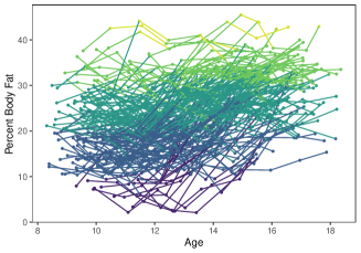
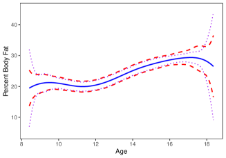
Figure 4: Left panel: percent body fat of 162 girls before and after menarche. Right panel: solid line: the estimated mean function using cubic B-splines; dashed line: the proposed SCB at the significance level of $95\%$; dotted line: the SCB developed in [11] at the significance level of $95\%$.

Figure 4 also shows that the estimated mean function of the percent body fat and the corresponding $95\%$ SCB, which indicates that percent body fat of girls gradually increases with age between 12 and 16 years old.

6.2 Dense case

The second dataset is accessible through the University of California, Irvine machine learning repository https://archive.ics.uci.edu/dataset/157/dodgers+loop+sensor. It was collected from a loop sensor for the Glendale on ramp for the $101$ North freeway in Los Angeles, located near Dodger Stadium, which is the home of the Los Angeles Dodgers baseball team. The sensor was designed to capture traffic volume, and it recorded measurements of the total number of cars every five minutes. For days when the Dodgers had a home game, additional details are available, including the time when the game started and ended.

This traffic data has been studied by [27], [38], while we are interested in the trend of car counts around the end of games on game days. For this purpose, we consider the end time of each game as the zero point ($t=0$) and focus on the car counts between $120$ minutes before the end ($t=-120$) and $120$ minutes after the game ($t=120$). The data we use spanned from April 2005 to October 2005 including 78 game days ($n=78$) with $\bar{N}=48.1$, which is illustrated in Figure 5.

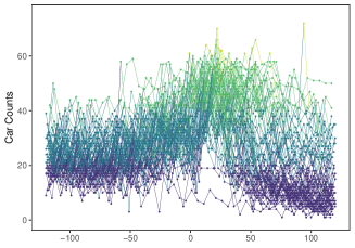
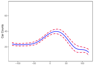
Figure 5: Left panel: car counts on 78 game days over 120 minutes before the end of a game until 120 minutes after the game. Right panel: solid line: the estimated mean function using cubic B-splines; dashed line: the proposed SCB at the significance level of $95\%$; dotted line: the SCB developed in [11] at the significance level of $95\%$.

Figure 5 also reveals that the car counts exhibits a unimodal shape, steadily rising and reaching its peak approximately $20$ minutes after the game and subsequently decreasing thereafter.

7 Concluding remark

In this paper, we present a unified framework for the simultaneous inference of mean functions, applicable irrespective of sampling strategy constraints. Our method involves the use of B-splines to construct SCBs, which are shown to be asymptotically valid from sparse to dense observations. We explore the behavior of the approximated Gaussian process to describe the phase transition phenomenon, balancing between the effect of ${\rm{Var}}(Y_{ij})$ and ${\rm{Cov}}(Y_{ij},Y_{ij^{\prime}})$. This meticulous analysis leads to categorizing samples as sparse, semi-dense, or dense. Notably, our results align with those in sparse and dense cases as discussed in [40] and [11], respectively. Moreover, our convergence rate approaches the optimal rate up to a logarithm term, offering a comparison to [9] and [2].

Furthermore, our methodology extends to orthogonal series estimators, achieving similar results with adjustments based on series-specific parameters. A significant advantage of our proposed SCB lies in its broader applicability compared to other SCBs, which are often constrained by sampling designs. This flexibility is particularly valuable in practical settings where determining the sparseness or denseness of a dataset is not straightforward.

Additionally, this framework’s potential applications extend beyond mean function estimation. It can be adapted for estimating other components, such as covariance functions and eigenfunctions, which involve multi-step nonparametric smoothing. Another promising avenue is its generalization to dependent functional data, which poses the intriguing challenge of estimating long-run covariance functions. These extensions represent both exciting and demanding prospects for future research in this field.

Supplementary Material

Supplementary Material contains detailed proofs of the theoretical results with necessarily technical lemmas

References

• Belloni etย al., [2015] Belloni, A., Chernozhukov, V., Chetverikov, D., and Kato, K. (2015). Some new asymptotic theory for least squares series: Pointwise and uniform results. Journal of Econometrics, 186(2):345โ€“366.
• Berger etย al., [2023] Berger, M., Hermann, P., and Holzmann, H. (2023). From dense to sparse design: Optimal rates under the supremum norm for estimating the mean function in functional data analysis. arXiv preprint arXiv:2306.04550.
• Berkes etย al., [2009] Berkes, I., Gabrys, R., Horvรกth, L., and Kokoszka, P. (2009). Detecting changes in the mean of functional observations. Journal of the Royal Statistical Society: Series B (Statistical Methodology), 71(5):927โ€“946.
• Bosq, [2000] Bosq, D. (2000). Linear processes in function spaces: theory and applications, volume 149. Springer Science & Business Media.
• [5] Cai, L. and Hu, Q. (2024+a). Global inference and test of eigen-systems of image data over complicated domain. Manusript.
• [6] Cai, L. and Hu, Q. (2024b). Simultaneous inference and uniform test for eigensystems of functional data. Computational Statistics & Data Analysis, 192:107900.
• [7] Cai, L. and Hu, Q. (2024+c). Simultaneous inference for distribution of functional principal scores. Manusript.
• Cai and Yuan, [2011] Cai, T.ย T. and Yuan, M. (2011). Optimal estimation of the mean function based on discretely sampled functional data: Phase transition. The Annals of Statistics, 39(5):2330 โ€“ 2355.
• Cai and Yuan, [2012] Cai, T.ย T. and Yuan, M. (2012). Minimax and adaptive prediction for functional linear regression. Journal of the American Statistical Association, 107(499):1201โ€“1216.
• Cao etย al., [2016] Cao, G., Wang, L., Li, Y., and Yang, L. (2016). Oracle-efficient confidence envelopes for covariance functions in dense functional data. Statistica Sinica, pages 359โ€“383.
• Cao etย al., [2012] Cao, G., Yang, L., and Todem, D. (2012). Simultaneous inference for the mean function based on dense functional data. Journal of nonparametric statistics, 24(2):359โ€“377.
• Chen, [2007] Chen, X. (2007). Large sample sieve estimation of semi-nonparametric models. Handbook of econometrics, 6:5549โ€“5632.
• Chen and Christensen, [2015] Chen, X. and Christensen, T.ย M. (2015). Optimal uniform convergence rates and asymptotic normality for series estimators under weak dependence and weak conditions. Journal of Econometrics, 188(2):447โ€“465.
• Cohen etย al., [1993] Cohen, A., Daubechies, I., and Vial, P. (1993). Wavelets on the interval and fast wavelet transforms. Applied and computational harmonic analysis.
• Cui and Zhou, [2022] Cui, Y. and Zhou, Z. (2022). Simultaneous inference for time series functional linear regression. arXiv preprint arXiv:2207.11392.
• DeVore and Lorentz, [1993] DeVore, R.ย A. and Lorentz, G.ย G. (1993). Constructive approximation, volume 303. Springer Science & Business Media.
• Ferraty and Vieu, [2006] Ferraty, F. and Vieu, P. (2006). Nonparametric functional data analysis: theory and practice, volumeย 76. Springer.
• Fitzmaurice etย al., [2012] Fitzmaurice, G.ย M., Laird, N.ย M., and Ware, J.ย H. (2012). Applied longitudinal analysis. John Wiley & Sons.
• Guo etย al., [2023] Guo, S., Li, D., Qiao, X., and Wang, Y. (2023). From sparse to dense functional data in high dimensions: Revisiting phase transitions from a non-asymptotic perspective. arXiv preprint arXiv:2306.00476.
• Hรคrdle, [1990] Hรคrdle, W. (1990). Applied nonparametric regression. Numberย 19. Cambridge university press.
• Hsing and Eubank, [2015] Hsing, T. and Eubank, R. (2015). Theoretical foundations of functional data analysis, with an introduction to linear operators, volume 997. John Wiley & Sons.
• [22] Hu, Q. and Li, J. (2024+a). Simultaneous inference for covariance function of next-generation functional data. Manusript.
• [23] Hu, Q. and Li, J. (2024b). Statistical inference for mean function of longitudinal imaging data over complicated domains. Statistica Sinica.
• Hu and Yang, [2024] Hu, Q. and Yang, L. (2024+). Statistical inference for multivariable functional data. Manuscript.
• Huang and Yang, [2004] Huang, J.ย Z. and Yang, L. (2004). Identification of non-linear additive autoregressive models. Journal of the Royal Statistical Society Series B: Statistical Methodology, 66(2):463โ€“477.
• Huang etย al., [2022] Huang, K., Zheng, S., and Yang, L. (2022). Inference for dependent error functional data with application to event-related potentials. TEST, 31(4):1100โ€“1120.
• Ihler etย al., [2006] Ihler, A., Hutchins, J., and Smyth, P. (2006). Adaptive event detection with time-varying poisson processes. In Proceedings of the 12th ACM SIGKDD international conference on Knowledge discovery and data mining, pages 207โ€“216.
• Li and Yang, [2023] Li, J. and Yang, L. (2023). Statistical inference for functional time series. Satisitica Sinica. DOI: 10.5705/ss.202021.0107.
• Li and Hsing, [2010] Li, Y. and Hsing, T. (2010). Uniform convergence rates for nonparametric regression and principal component analysis in functional/longitudinal data. The Annals of Statistics, 38(6):3321โ€“3351.
• Mies and Steland, [2023] Mies, F. and Steland, A. (2023). Sequential gaussian approximation for nonstationary time series in high dimensions. Bernoulli, 29(4):3114โ€“3140.
• Phillips etย al., [2003] Phillips, S.ย M., Bandini, L.ย G., Compton, D.ย V., Naumova, E.ย N., and Must, A. (2003). A longitudinal comparison of body composition by total body water and bioelectrical impedance in adolescent girls. The Journal of nutrition, 133(5):1419โ€“1425.
• Quan and Lin, [2022] Quan, M. and Lin, Z. (2022). Optimal one-pass nonparametric estimation under memory constraint. Journal of the American Statistical Association, pages 1โ€“12.
• Sharghi Ghale-Joogh and Hosseini-Nasab, [2021] Sharghi Ghale-Joogh, H. and Hosseini-Nasab, S. M.ย E. (2021). On mean derivative estimation of longitudinal and functional data: from sparse to dense. Statistical Papers, 62(4):2047โ€“2066.
• Wang etย al., [2020] Wang, J., Cao, G., Wang, L., and Yang, L. (2020). Simultaneous confidence band for stationary covariance function of dense functional data. Journal of Multivariate Analysis, 176:104584.
• [35] Yao, F., Mรผller, H.-G., and Wang, J.-L. (2005a). Functional data analysis for sparse longitudinal data. Journal of the American statistical association, 100(470):577โ€“590.
• [36] Yao, F., Mรผller, H.-G., and Wang, J.-L. (2005b). Functional linear regression analysis for longitudinal data. The Annals of Statistics, 33(6):2873โ€“2903.
• Zhang and Li, [2022] Zhang, H. and Li, Y. (2022). Unified principal component analysis for sparse and dense functional data under spatial dependency. Journal of Business & Economic Statistics, 40(4):1523โ€“1537.
• Zhang and Wang, [2015] Zhang, X. and Wang, J.-L. (2015). Varying-coefficient additive models for functional data. Biometrika, 102(1):15โ€“32.
• Zhang and Wang, [2016] Zhang, X. and Wang, J.-L. (2016). From sparse to dense functional data and beyond. The Annals of Statistics, 44:2281โ€“2321.
• Zheng etย al., [2014] Zheng, S., Yang, L., and Hรคrdle, W.ย K. (2014). A smooth simultaneous confidence corridor for the mean of sparse functional data. Journal of the American Statistical Association, 109(506):661โ€“673.
• Zygmund, [2002] Zygmund, A. (2002). Trigonometric series. Cambridge university press.