Marginal treatment effects in the absence of instrumental variables

Abstract

We propose a method for defining, identifying, and estimating the marginal treatment effect (MTE) without imposing the instrumental variable (IV) assumptions of independence, exclusion, and separability (or monotonicity). Under a new definition of the MTE based on reduced-form treatment error that is statistically independent of the covariates, we find that the relationship between the MTE and standard treatment parameters holds in the absence of IVs. We provide a set of sufficient conditions ensuring the identification of the defined MTE in an environment of essential heterogeneity. The key conditions include a linear restriction on potential outcome regression functions, a nonlinear restriction on the propensity score, and a conditional mean independence restriction that will lead to additive separability. We prove this identification using the notion of semiparametric identification based on functional form. We suggest consistent semiparametric estimation procedures, and provide an empirical application for the Head Start program to illustrate the usefulness of the proposed method in analyzing heterogenous causal effects when IVs are elusive.

Keywords: causal inference; treatment effect heterogeneity; identification based on functional form; Head Start

JEL Codes: C14, C31, C51

1 Introduction

The marginal treatment effect (MTE), which was developed in a series of seminal papers by Heckman and Vytlacil (1999, 2001, 2005), has become one of the most popular tools in social sciences for describing, interpreting, and analyzing the heterogeneity of the effect of a nonrandom treatment. The MTE is defined as the expected treatment effect conditional on the observed covariates and normalized error term consisting of unobservable determinants of the treatment status. Although the definition of MTE does not necessitate an instrumental variable (IV), nearly all the existing identification strategies for the MTE rely heavily on valid instrumental variation that can induce otherwise similar individuals into different treatment choices. This is mainly because the MTE has been regarded as an extension of and supplement to the standard IV method in the causal inference literature. In the most common case of just-identification, in which only one IV is available, the exogeneity or randomness of the IV is fundamentally untestable and usually informally verified by regressing the IV on a set of pretreatment characteristics. However, a large body of empirical studies presented at least weak evidence against the (conditional) randomness of the IV in use (e.g., Arnold et al., 2018; Cornelissen et al., 2018; Kamhöfer et al., 2019; Fischer et al., 2020; Mountjoy, 2022; Westphal et al., 2022). The exclusion restriction, which is another condition underlying the validity of IV, has also been challenged more often than not (e.g., Jones, 2015).

Motivated by the potential invalidity of the available instruments, and inspired by the observation that instruments are not necessary in the definition of MTE, we model, identify, and estimate the MTE without imposing the standard IV assumptions of conditional independence, exclusion, and separability. Namely, we allow all the observed covariates to be statistically correlated to the error term and have a direct impact on the outcome in addition to an indirect impact through the treatment variable. The cornerstone of our model is a normalized treatment equation, which determines treatment participation by the propensity score crossing a reduced-form error term that is statistically independent of (although functionally dependent on) all the covariates. This is comparable to the conventional IV model, in which normalization is performed with respect to only the non-IV covariates. The independence of the reduced-form treatment error from all the covariates can partly justify a conditional mean independence assumption on the potential outcome residuals, which can ensure the additive separability of the MTE into observables and unobservables. This separability then facilitates the semiparametric identification of the MTE, given a linear restriction on the potential outcome regression functions and a nonlinear restriction on the propensity score function. We prove the identification by representing the MTE as a known function of conditional moments of observed variables. Intuitively, the identification power comes from the excluded nonlinear variation in the propensity score, which plays the role of the IV in exogenously perturbing the treatment status. Our identification strategy closely resembles the semiparametric counterpart of identification based on functional form (Dong, 2010; Escanciano et al., 2016; Lewbel, 2019; Pan et al., 2022). We build our result on the notion of identification based on functional form mainly because (i) it can lead to point identification and estimation, (ii) the required assumptions are regular, and (iii) the resulting estimation procedures are the most compatible with the standard procedures in conventional IV-MTE models. After identification, the MTE can be semiparametrically estimated by implementing the kernel-weighted pairwise difference regression for the sample selection model (Ahn and Powell, 1993) for each treatment status.

We contribute to the literature on program evaluation under essential heterogeneity by proposing a method for defining, identifying, and estimating the MTE in the absence of IVs. The main value of this IV-free framework of the MTE is threefold. First, it provides an approach for consistently estimating heterogeneous causal effects when valid IVs are difficult to find. Second, it suggests an easy-to-implement means for testing the validity of a candidate IV, because it nests the models that assume exclusion restrictions. For instance, in studies on returns to education, the validity of most of the proposed instruments for educational attainment is suspect, such as parental education, distance to the school, and local labor market conditions (Kédagni and Mourifié, 2020; Mourifié et al., 2020). Our framework enables the reliable evaluation of returns to education without imposing IV assumptions on the candidate instruments and implies a simple test for exclusion restrictions by $t$-testing the instruments’ coefficients in potential outcome equations. Third, even though the validity of the IV is verified, identification based on functional form can be invoked as a way to increase the efficiency of estimation or to check the robustness of the results to alternative identifying assumptions.

Early explorations of the identification of endogenous regression models when IVs are unavailable focused on linear systems of simultaneous equations, in which the lack of IVs is associated with hardly justifiable exclusion restrictions and insufficient moment conditions. The typical strategy for addressing this underidentification problem is to impose second- or higher-order moment restrictions to construct instruments by using the available exogenous covariates (e.g., Lewbel, 1997; Klein and Vella, 2010). In particular, imposing restrictions on the correlation between the covariates and the variance matrix of the vector of model errors leads to identification based on heteroscedasticity (Lewbel, 2012). We refer the reader to Lewbel (2019) for a comprehensive review of this approach. D’Haultfœuille et al. (2021) considered a nonlinear triangular model without the exclusion restriction and established identification for the control function approach based on a local irrelevance condition. The above results are restricted to the case of continuously valued endogenous variable or treatment. Lewbel (2018) showed that in linear regression models, the moment conditions of identification based on heteroscedasticity can be satisfied when the endogenous treatment is binary, at the expense of strong restrictions on the model errors. Alternatively, Conley et al. (2012) and Van Kippersluis and Rietveld (2018) presented a sensitivity analysis approach for performing inference for linear IV models while relaxing the exclusion restriction to a certain extent. However, the linear models implicitly impose an undesirable homogeneity assumption on treatment effects.

The literature on sample selection models without the exclusion restriction is also closely related. A general solution to the problem of lack of excluded variables is partial identification and set estimation (Honoré and Hu, 2020, 2022; Westphal et al., 2022). The limitation of this approach is that the identified or estimated set may be too wide to be informative. Another solution is the approach of identification at infinity that uses the data only for large values of a special regressor (Chamberlain, 1986; Lewbel, 2007) or of the outcome (D’Haultfœuille and Maurel, 2013; D’Haultfœuille et al., 2018). Although identification at infinity can lead to point identification, it is typically featured as irregular identification (Khan and Tamer, 2010), and the derived estimate will converge at a rate slower than $n^{-1/2}$, where $n$ is the sample size. Heckman (1979) exploited nonlinearity in the selectivity correction function to achieve point identification and root-$n$ consistent estimation for the linear coefficients of a parametric sample selection model, which is the original version of identification based on functional form. However, Heckman’s model imposes a restrictive bivariate normality assumption on the error terms and thus poses the risk of model misspecification. Escanciano et al. (2016) extended Heckman’s approach to a general semiparametric model and established identification of the linear coefficients by exploiting nonlinearity elsewhere in the model. At the expense of the generality of their model, Escanciano et al. (2016)’s identification result was only up to scale and required a scale normalization assumption. This normalization would be innocuous if we know the sign of the normalized coefficient and are interested in only the sign, but not the magnitude, of the other coefficients. However, the magnitude of the linear coefficients is indispensable to the evaluation of a program or a policy. In addition, the identification assumption about nonlinearity developed by Escanciano et al. (2016) implicitly rules out the case of the existence of two continuous covariates. We adapt the result of Escanciano et al. (2016) to the MTE model by amending the two defects. First, we take advantage of the specific model structure to relax the scale normalization and identify the magnitude of the linear coefficients. Moreover, the identifying assumption about nonlinearity will be simplified owing to the specific model structure. We give an intuitive interpretation of the new nonlinearity assumption. Second, we combine the nonlinearity assumption with a local irrelevance condition to allow for an arbitrary number of continuous covariates.

The rest of this paper is organized as follows. In Section 2, we introduce our model and the definition of the MTE without IVs. In Section 3, we propose a possible set of sufficient conditions for the identification of the MTE, in place of the standard IV assumptions. The key conditions include semiparametric functional form restrictions and the conditional mean independence assumption, of which the latter implies the additive separability of the MTE into observed and unobserved components. In Section 4, we suggest consistent estimation procedures, and in Section 5, we provide an empirical application to Head Start. Section 6 concludes. The Appendix contains the detailed proof of the main identification result, a discussion on the variants of the nonlinearity assumption, and an identification result for limited valued outcomes that entails a slight modification of the assumptions.

2 Model

In the following, we denote random variables or random vectors by capital letters, such as $U$, and their possible realizations by the corresponding lowercase letters, such as $u$. We denote $F_{U}\left(\cdot\right)$ as the cumulative distribution function (CDF) of $U$ and $F_{U\left|X\right.}\left(\cdot\left|x\right.\right)$ as the conditional CDF of $U$ given $X=x$. Our analysis builds on the potential outcomes framework developed by Roy (1951) in econometrics and Rubin (1973a, b) in statistics. Specifically, we consider a binary treatment, denoted by $D$, and let $Y_{1}$ and $Y_{0}$ denote the potential outcomes if the individuals are treated ($D=1$) or not treated ($D=0$), respectively. The observed outcome is

$$Y=DY_{1}+\left(1-D\right)Y_{0},$$

and the quantity of interest is the counterfactual treatment effect

$$\Delta=Y_{1}-Y_{0}.$$

We suppose that the treatment status is determined by the following threshold crossing rule:

$$D=1\left\{\mu\left(X\right)\geq U\right\},$$ (1)

where $X$ is a vector of pretreatment covariates, $1\left\{A\right\}$ is the indicator function of event $A$, $\mu\left(\cdot\right)$ is an unknown function, and $U$ is a structural error term containing unobserved characteristics that may affect participation in the treatment, such as the opportunity costs or intangible benefits of the treatment.

Compared with the conventional MTE model, we relax the independence and separability assumptions in the treatment equation (1) to account for the absence of IVs. First, we do not assume that $X$ is stochastically independent of $U$; that is, no exogenous covariate is needed. Second, we allow the treatment decision rule to be intrinsically nonseparable in observed and unobserved characteristics, which is equivalent to relaxing the monotonicity assumption in the IV model (Vytlacil, 2002, 2006). Specifically, let $U_{x}$ be the counterfactual error term denoting what $U$ would have been if $X$ had been externally set to $x$, then the nonseparability of (1) means that at least two vectors $x$ and $\tilde{x}$ exist in the support of $X$ such that $U_{x}\neq U_{\tilde{x}}$ with positive probability. In particular, $U$ is allowed to depend functionally on $X$, as in the following example.

Example 1.

We consider a latent index rule for treatment participation:

$$D=1\left\{m\left(X,\varepsilon\right)\geq 0\right\},$$ (2)

where the observed $X$ can be statistically correlated to the unobserved $\varepsilon$, and no restriction is imposed on the cross-partials of the index function $m$. Without independence and additive separability, model (2) is completely vacuous, imposing no restrictions on the observed or counterfactual outcomes (Heckman and Vytlacil, 2001). This general latent index rule fits into the threshold crossing rule (1) by taking $\mu\left(X\right)=E\left[m\left(X,\varepsilon\right)\left|X\right.\right]$ and $U=\mu\left(X\right)-m\left(X,\varepsilon\right)$.

Example 1 illustrates that no generality is lost by modeling the treatment variable as equation (1) without imposing the independence and separability assumptions. We define the propensity score function as the conditional probability of receiving the treatment given the covariates,

$$\pi\left(x\right)\equiv E\left[D\left|X=x\right.\right]=F_{U\left|X\right.}\left(\mu\left(x\right)\left|x\right.\right),$$

and define the propensity score variable as $P\equiv\pi\left(X\right)$. Under the regularity condition that $F_{U\left|X\right.}\left(\cdot\left|x\right.\right)$ is absolutely continuous with respect to the Lebesgue measure for all $x$, the structural treatment equation (1) can be innocuously normalized into a reduced form:

$$D=1\left\{P\geq V\right\},$$ (3)

where

$$V=F_{U\left|X\right.}\left(U\left|X\right.\right)$$

is a normalized error term, which by definition follows standard uniform distribution conditional on $X$ and thus is stochastically independent of $X$ and $P$. This independence, which seems counterintuitive owing to the functional dependence of $V$ on $X$, is lost if we consider $V_{x}=F_{U\left|X\right.}\left(U_{x}\left|x\right.\right)$, the counterfactual variable of $V$ when $X$ is set to $x$. In general, the conditional distribution of $V_{x}$ given $X=\tilde{x}$ for $\tilde{x}\neq x$ depends on $\tilde{x}$, and the unconditional distribution of $V_{x}$ is no longer uniform.

Example 2.

We suppose that $X$ is a scalar, and

$$\left(\begin{array}[]{l}U\\ X\end{array}\right)\sim N\left(\left(\begin{array}[]{l}0\\ 0\end{array}\right),\left(\begin{array}[]{cc}1&\sigma_{UX}\\ \sigma_{UX}&\sigma_{X}^{2}\end{array}\right)\right).$$

Through a property of the bivariate normal distribution, we obtain $U\left|\left(X=x\right)\right.\sim N\left(\mu_{\left.U\right|X}\left(x\right),\sigma_{U\left|X\right.}^{2}\right)$ and $F_{U\left|X\right.}\left(u\left|x\right.\right)=\Phi\left(\left.\left[u-\mu_{U\left|X\right.}\left(x\right)\right]\right/\sigma_{U\left|X\right.}\right)$, where $\mu_{U\left|X\right.}\left(x\right)=\left(\sigma_{UX}\left/\sigma_{X}^{2}\right.\right)x$, $\sigma_{U\left|X\right.}^{2}=1-\left(\sigma_{UX}^{2}\left/\sigma_{X}^{2}\right.\right)$, and $\Phi\left(\cdot\right)$ denotes the standard normal CDF. Hence,

$$V=F_{U\left|X\right.}\left(U\left|X\right.\right)=\Phi\left(\frac{U-\mu_{U\left|X\right.}\left(X\right)}{\sigma_{U\left|X\right.}}\right)\text{, and }V_{x}=\Phi\left(\frac{U-\mu_{U\left|X\right.}\left(x\right)}{\sigma_{U\left|X\right.}}\right).$$

We observe that $V\perp\!\!\!\!\perp X$ because $F_{V\left|X\right.}\left(v\left|x\right.\right)=v$, but $V_{x}\leavevmode\hbox{\hbox to0.0pt{\thinspace/\hss}{$\perp\!\!\!\!\perp$}}X$ because

$$F_{V_{x}\left|X\right.}\left(v\left|\tilde{x}\right.\right)=\Phi\left(\frac{\left(\sigma_{UX}\left/\sigma_{X}^{2}\right.\right)\left(x-\tilde{x}\right)}{\sigma_{U\left|X\right.}}+\Phi^{-1}\left(v\right)\right),$$

and $V_{x}$ is not uniformly distributed because $F_{V_{x}}\left(v\right)=\Phi\left(\mu_{U\left|X\right.}\left(x\right)+\sigma_{U\left|X\right.}\Phi^{-1}\left(v\right)\right)$.

Given this independence, we may consider the reduced-form treatment error $V$ as the orthogonalized unobservables with respect to the observables, or the unobservables that are projected onto the subspace orthogonal to the one spanned by the observables. Another interpretation of $V$ is the ranking of the structural error $U$ conditional on $X$. For instance, $V=0.2$ represents a typical individual whose $U$ value ranks above 20% individuals with identical covariates. $V$ enters the normalized crossing rule on the right, making an individual less likely to receive treatment; thus, it refers to resistance or distaste regarding the treatment in the MTE literature. If $V$ is large, then the propensity score $P$ should be large to induce the individual to participate in the treatment. However, an individual with a $V$ value close to zero will participate even though $P$ is small.

In the above instrument-free model, we define the MTE as the expected treatment effect conditional on the observed and unobserved characteristics:

$$\Delta^{\text{MTE}}\left(x,v\right)\equiv E\left[\left.\Delta\right|X=x,V=v\right].$$

$\Delta^{\text{MTE}}\left(x,v\right)$ captures all the treatment effect heterogeneity that is consequential for selection bias by conditioning on the orthogonal coordinates of the observable and unobservable dimensions. Given $X$ and $V$, the treatment status $D$ is fixed and thus independent of the treatment effect $\Delta$. Similar to the MTE in the IV model, $\Delta^{\text{MTE}}\left(x,v\right)$ can be used as a building block for constructing the commonly used causal parameters, such as the average treatment effect (ATE), the treatment effect on the treated (TT), the treatment effect on the untreated (TUT), and the local average treatment effect (LATE), which can be expressed as weighted averages of $\Delta^{\text{MTE}}\left(x,v\right)$, as follows:

$$\Delta^{\text{ATE}}\left(x\right) \equiv E\left[\left.\Delta\right|X=x\right]=\int_{0}^{1}\Delta^{\text{MTE}}\left(x,v\right)dv,$$

$$\Delta^{\text{TT}}\left(x\right) \equiv E\left[\left.\Delta\right|X=x,D=1\right]=\frac{1}{\pi\left(x\right)}\int_{0}^{\pi\left(x\right)}\Delta^{\text{MTE}}\left(x,v\right)dv,$$

$$\Delta^{\text{TUT}}\left(x\right) \equiv E\left[\left.\Delta\right|X=x,D=0\right]=\frac{1}{1-\pi\left(x\right)}\int_{\pi\left(x\right)}^{1}\Delta^{\text{MTE}}\left(x,v\right)dv,$$

$$\Delta^{\text{LATE}}\left(x,v_{1},v_{2}\right) \equiv E\left[\left.\Delta\right|X=x,v_{1}\leq V\leq v_{2}\right]=\frac{1}{v_{2}-v_{1}}\int_{v_{1}}^{v_{2}}\Delta^{\text{MTE}}\left(x,v\right)dv.$$

Somewhat surprisingly, compared with the weights on the conventional MTE (e.g., Heckman and Vytlacil, 2005, Table IB), which are generally difficult to estimate in practice, the weights on $\Delta^{\text{MTE}}\left(x,v\right)$ are simpler, more intuitive, and easier to compute.

Heckman and Vytlacil (2001, 2005) considered defining the MTE in a similar nonseparable setting by conditioning on the structural error $U$ in (1) or $\varepsilon$ in (2), and showed how to integrate to generate other causal parameters. However, such an MTE cannot be identified even in the presence of IVs. Our definition, based on the reduced-form error $V$ in (3), can effectively exploit the statistical independence of the observed and unobserved variables to facilitate identification of the MTE. Zhou and Xie (2019) proposed redefining the MTE as the expected treatment effect given $P$ and $V$, which is a more parsimonious specification of all the relevant treatment effect heterogeneity for selection bias. The extension of our identification and estimation procedures to this alternative definition is straightforward.

3 Identification

Our identification strategy relies on a linearity restriction on the potential outcome equations and a nonlinearity restriction on the propensity score function. The intuition is that the propensity score minus the linear outcome index will provide the excluded variation perturbing treatment status, which plays the role of a continuous IV. Furthermore, to ensure the exogeneity of the nonlinear variation, it is necessary to impose a certain form of independence between the covariates and potential outcome residuals. Specifically, we make the following assumptions to achieve the identification of $\Delta^{\text{MTE}}\left(x,v\right)$. Before proceeding, we create additional notations. We let $X$ be partitioned as $\left(X^{C},X^{D}\right)$, where $X^{C}$ and $X^{D}$ consist of covariates that are continuously and discretely distributed, respectively. Without loss of generality, we suppose that the vector of zeros is in the support of $X^{D}$. Denote $X_{k}$, $X_{k}^{C}$, and $X_{k}^{D}$ as the $k$-th coordinates of $X$, $X^{C}$, and $X^{D}$, respectively. Denote $x^{C}$ as a generic element in the support of $X^{C}$; likewise for $x^{D}$, $x_{k}^{C}$, and $x_{k}^{D}$. Moreover, denote $\pi_{0}\left(x^{C}\right)=\pi\left(x^{C},0\right)$, where the discrete covariates are equal to zero. If $\pi_{0}$ is differentiable at $x^{C}$, then we denote $\partial_{k}\pi_{0}\left(x^{C}\right)=\left.\partial\pi_{0}\left(x^{C}\right)\right/\partial x_{k}^{C}$ as its partial derivative with respect to the $k$-th argument. For any $x^{D}$, we denote $x^{Dk}$ as the $\dim\left(x^{D}\right)\times 1$ vector with the $k$-th coordinate being equal to $x_{k}^{D}$ and all the other coordinates being equal to zero.

Assumption L (Linearity). Assume that $E\left[\left.Y_{d}\right|X=x\right]=\alpha_{d}+x^{\prime}\beta_{d}$ for some fixed $\alpha_{d}$ and $\beta_{d}$, $d=0,1$.

Assumption NL (Non-Linearity). Assume that $\pi_{0}$ satisfies the following NL1 when $\dim\left(X^{C}\right)=1$ or NL2 when $\dim\left(X^{C}\right)\geq 2.$

– NL1 ($\dim\left(X^{C}\right)=1$): there exist two different constants $x^{C}$, $\tilde{x}^{C}$ in the support of $X^{C}$ such that $\pi_{0}\left(x^{C}\right)=\pi_{0}\left(\tilde{x}^{C}\right)$.

– NL2 ($\dim\left(X^{C}\right)\geq 2$): there exist two vectors $x^{C}$, $\tilde{x}^{C}$ in the support of $X^{C}$ and two elements $k$, $j$ in set $\left\{1,2,\cdots,\dim\left(X^{C}\right)\right\}$ such that $\pi_{0}$ and $E\left[Y\left|X^{C}=x^{C},X^{D}=0,D=d\right.\right]$, $d=0,1$, are differentiable at $x^{C}$ and $\tilde{x}^{C}$, and that (i) $\partial_{k}\pi_{0}\left(x^{C}\right)\neq 0$, (ii) $\partial_{j}\pi_{0}\left(x^{C}\right)\neq 0$, (iii) $\partial_{k}\pi_{0}\left(\tilde{x}^{C}\right)\neq 0$, (iv) $\partial_{j}\pi_{0}\left(\tilde{x}^{C}\right)\neq 0$, and (v) $\left.\partial_{k}\pi_{0}\left(x^{C}\right)\right/\partial_{j}\pi_{0}\left(x^{C}\right)\neq\left.\partial_{k}\pi_{0}\left(\tilde{x}^{C}\right)\right/\partial_{j}\pi_{0}\left(\tilde{x}^{C}\right)$.

Assumption CMI (Conditional Mean Independence). Denote $U_{d}=Y_{d}-X^{\prime}\beta_{d}$, $d=0,1$. Assume that $E\left[U_{d}\left|V,X\right.\right]=E\left[U_{d}\left|V\right.\right]$ with probability one for $d=0,1$.

Assumption S (Support). For each $k\in\left\{1,2,\cdots,\dim\left(X^{D}\right)\right\}$, assume for some $x_{k}^{D}\neq 0$ in the support of $X_{k}^{D}$ that there exists $x^{C}\left(k\right)$ in the support of $X^{C}$ such that $\pi\left(x^{C}\left(k\right),x^{Dk}\right)$ is in the support of $\pi_{0}\left(X^{C}\right)$.

Assumption L imposes a linear restriction on the potential outcome regression functions, which is a common practice in empirical studies. The linear restriction may seem too strong compared with that in the existing identification strategies, which allow highly flexible (especially nonparametric) specifications on the potential outcomes. However, for the estimation of the MTE, the linear specification has been nearly universally adopted for tractability and interpretability (e.g., Kirkeboen et al., 2016; Kline and Walters, 2016; Brinch et al., 2017; Heckman et al., 2018; Mogstad et al., 2021; Aryal et al., 2022; Mountjoy, 2022). Noting that Assumption L implicitly requires the potential outcomes to be continuously distributed and supported on the entire real line, we would like to point out that our identification strategy can also be adapted to the case of limited valued outcomes by specifying linear latent index. A detailed discussion is left to Appendix A.3.

By contrast, Assumption NL requires the propensity score function to be nonlinear in the continuous covariates in a generalized sense. The combination of Assumptions L and NL will enable identification based on functional form in a semiparametric version that can realize the identification of linear coefficients by exploiting nonlinearity elsewhere in the model. The nonlinearity assumption has two different forms, depending on the number of continuous covariates. When two or more continuous covariates are available, Assumption NL2 will require some variation in $\pi_{0}$ to distinguish it from a linear index function. Concretely, NL2 will not hold if $\pi_{0}\left(x^{C}\right)=f\left(x^{C\prime}\gamma\right)$ for a smooth function $f$, because in this case, both sides of the inequality in (v) are equal to $\left.\gamma_{k}\right/\gamma_{j}$. Otherwise, however, it is difficult to construct examples that violate (v). In practice, (v) can be fulfilled even when $\pi_{0}$ is single-index specified, if interaction or/and quadratic terms are added, as shown in Example 3.

Example 3.

Consider the case of two continuous covariates. Suppose that for a smooth function $f$, $\pi_{0}\left(x^{C}\right)=f\left(\gamma_{1}x_{1}^{C}+\gamma_{2}x_{2}^{C}+\gamma_{3}x_{1}^{C}x_{2}^{C}\right)$ or $\pi_{0}\left(x^{C}\right)=f\left(\gamma_{1}x_{1}^{C}+\gamma_{2}x_{2}^{C}+\gamma_{3}\left(x_{1}^{C}\right)^{2}\right)$. Then, we obtain $\left.\partial_{1}\pi_{0}\left(x^{C}\right)\right/\partial_{2}\pi_{0}\left(x^{C}\right)=\left.\left(\gamma_{1}+\gamma_{3}x_{2}^{C}\right)\right/\left(\gamma_{2}+\gamma_{3}x_{1}^{C}\right)$ for the interaction case, or $\left.\partial_{1}\pi_{0}\left(x^{C}\right)\right/\partial_{2}\pi_{0}\left(x^{C}\right)=\left.\left(\gamma_{1}+2\gamma_{3}x_{1}^{C}\right)\right/\gamma_{2}$ for the quadratic case. In both cases, Assumption NL2 (v) will generally hold for $x^{C}$ and $\tilde{x}^{C}$ satisfying $x_{1}^{C}\neq\tilde{x}_{1}^{C}$.

Assumption NL2 requires the existence of at least two continuous covariates. However, in empirical studies based on survey data, most of the demographic characteristics are documented as discrete or categorical variables, such as age, gender, race, marital status, educational attainment, and so on. Therefore, we also impose Assumption NL1, as a supplement to NL2, to take into account the situation in which only one continuous covariate is available. NL1 requires the univariate function $\pi_{0}$ to be not one-to-one, but imposes no other smoothness or continuity restriction on $\pi_{0}$. This condition will hold if the probability of receiving treatment is unaffected by some change in the continuous covariate. A similar local irrelevance assumption is imposed in nonseparable models to attain point identification (Torgovitsky, 2015) or to test and relax the exclusion restriction (D’Haultfœuille et al., 2021). Following the line of Assumption NL1, our identification strategy works even when no continuous covariate is available in the data, and we put a discretely distributed covariate in $X^{C}$. In the extreme case of $X^{C}$ containing only one binary covariate, NL1 will be equivalent to the full irrelevance of $X^{C}$ to the treatment probability, which is a condition suggested by Chamberlain (1986) in the identification of the sample selection model. However, using only discrete covariates provides little identifying variation, which may lead to poor performance in the subsequent model estimation (Garlick and Hyman, 2022). Hence, we focus on the case of at least one continuous covariate. We also note that if $\pi_{0}$ is assumed to be differentiable as in NL2, then the local irrelevance condition can be rephrased as a simpler form and extended to multiple continuous covariates. Further discussion on NL1 and its variants is left to Appendix A.2.

The nonlinearity assumption does not exclude the widely specified linear-index treatment equation

$$D=1\left\{X^{\prime}\gamma\geq U\right\},$$

as long as the structural error $U$ is not independent of $X$. For instance, consider a multiplicatively heteroscedastic $U$ such that $U=\sigma\left(X\right)\tilde{U}$, where $\sigma\left(X\right)$ is a positive function and $\tilde{U}$ is an idiosyncratic error independent of $X$. The normalization derives

$$D=1\left\{\frac{X^{\prime}\gamma}{\sigma\left(X\right)}\geq\tilde{U}\right\},$$

that is, the reduced-form error $V$ in (3) is equal to $\tilde{U}$, and the propensity score function is equal to $\pi\left(x\right)=\left.\left(x^{\prime}\gamma\right)\right/\sigma\left(x\right)$. In general, $\pi\left(x\right)$ is a nonlinear function. Another example is a linear model with endogeneity in a certain component $X^{e}$ of $X^{C}$, in which $\pi\left(x\right)=F_{U\left|X^{e}\right.}\left(\left.x^{\prime}\gamma\right|x^{e}\right)$. Given that $\pi\left(x\right)$ is generally highly nonlinear in $x^{e}$, Assumption NL1 holds straightforwardly, and NL2 holds with $x_{k}^{C}=x^{e}$. Unlike in the binary response model, the ubiquitous heteroscedasticity and endogeneity benefit our results while inducing no trouble, because the identification of the MTE is irrelevant to the structural coefficient $\gamma$. Our MTE is defined by the reduced-form treatment error; thus, all we need from the treatment equation is the propensity score, which has a reduced-form nature.

Assumption CMI is standard in the MTE literature and commonly referred to as the separability or additive separability assumption (e.g., Brinch et al., 2017; Mogstad et al., 2018; Zhou and Xie, 2019), because it renders the MTE additively separable into observables and unobservables:

$$\Delta^{\text{MTE}}\left(x,v\right)=x^{\prime}\left(\beta_{1}-\beta_{0}\right)+E\left[U_{1}-U_{0}\left|V=v\right.\right].$$

Therefore, this assumption implies that the shape of the MTE curve will not vary with covariates. By definition, $E\left[U_{d}\left|X\right.\right]=\alpha_{d}=E\left[U_{d}\right]$, and $V\perp\!\!\!\!\perp X$; hence, Assumption CMI essentially requires the conditional covariance of $U_{d}$ and $V$ to be independent of $X$, which is also a key assumption in the heteroscedasticity-based identification method (Lewbel, 2012). This assumption can provide an alternative source of exogenous excluded variation for the identification in place of the IV. It is implied by and much weaker than the full independence $\left(U_{d},U\right)\perp\!\!\!\!\perp X$, which is frequently imposed (often implicitly) in applied work, where $U$ is the structural treatment error in (1). In particular, Assumption CMI does not rule out the marginal dependence of $U_{d}$ or $U$ on $X$, as illustrated in Example 4. Assumption S imposes a mild support condition for technical reasons. A sufficient condition for Assumption S to hold is if $\pi_{0}\left(X^{C}\right)$ has full support on the unit interval.

Example 4.

Suppose that $X$ is a scalar and

$$\left(\begin{array}[]{c}U_{d}\\ U\\ X\end{array}\right)\sim N\left(\left(\begin{array}[]{c}0\\ 0\\ 0\end{array}\right),\left(\begin{array}[]{ccc}\sigma_{d}^{2}&\sigma_{dU}&0\\ \sigma_{dU}&1&\sigma_{UX}\\ 0&\sigma_{UX}&\sigma_{X}^{2}\end{array}\right)\right).$$

In this setting, $U$ is correlated to $X$. Through a property of the multivariate normal distribution, we obtain

$$\left.\left(\begin{array}[]{c}U_{d}\\ U\end{array}\right)\right|\left(X=x\right)\sim N\left(\left(\begin{array}[]{c}0\\ \mu_{\left.U\right|X}\left(x\right)\end{array}\right),\left(\begin{array}[]{cc}\sigma_{d}^{2}&\sigma_{dU}\\ \sigma_{dU}&\sigma_{U\left|X\right.}^{2}\end{array}\right)\right),$$ (4)

where $\mu_{U\left|X\right.}\left(x\right)=\left(\sigma_{UX}\left/\sigma_{X}^{2}\right.\right)x$ and $\sigma_{U\left|X\right.}^{2}=1-\left(\sigma_{UX}^{2}\left/\sigma_{X}^{2}\right.\right)$. Hence,

$$E\left[\left.U_{d}\right|U=u,X=x\right]=\frac{\sigma_{dU}}{\sigma_{U\left|X\right.}^{2}}\left(u-\mu_{\left.U\right|X}\left(x\right)\right).$$

By Example 2, we have $V=\Phi\left(\left.\left[U-\mu_{U\left|X\right.}\left(X\right)\right]\right/\sigma_{U\left|X\right.}\right)$, so that $U=\sigma_{U\left|X\right.}\Phi^{-1}\left(V\right)+\mu_{U\left|X\right.}\left(X\right)$. Consequently,

$$E\left[\left.U_{d}\right|V=v,X=x\right]=E\left[\left.U_{d}\right|U=\sigma_{U\left|X\right.}\Phi^{-1}\left(v\right)+\mu_{U\left|X\right.}\left(x\right),X=x\right]=\frac{\sigma_{dU}}{\sigma_{U\left|X\right.}}\Phi^{-1}\left(v\right),$$

and Assumption CMI holds. More generally, to allow the dependence of $U_{d}$ on $X$ as well, we can set

$$\left.\left(\begin{array}[]{c}U_{d}\\ U\end{array}\right)\right|\left(X=x\right)\sim N\left(\left(\begin{array}[]{c}0\\ \mu_{\left.U\right|X}\left(x\right)\end{array}\right),\left(\begin{array}[]{cc}\sigma_{d}^{2}\left(x\right)&\sigma_{dU}\\ \sigma_{dU}&\sigma_{U\left|X\right.}^{2}\end{array}\right)\right)$$

in place of (4), where $\sigma_{d}^{2}\left(x\right)$ is the conditional variance of $U_{d}$ given $X=x$. Since $E\left[\left.U_{d}\right|V=v,X=x\right]$ is irrelevant to the variance of $U_{d}$ according to the above analysis, Assumption CMI still holds in the presence of such heteroscedastic $U_{d}$.

Under Assumptions L and CMI, we have

$$E\left[Y\left|X=x,D=d\right.\right]=x^{\prime}\beta_{d}+g_{d}\left(\pi\left(x\right)\right)$$ (5)

for $d=0,1$, where

$$g_{0}\left(p\right) = E\left[\left.U_{0}\right|V>p\right]=\frac{1}{1-p}\int_{p}^{1}E\left[\left.U_{0}\right|V=v\right]dv,$$

$$g_{1}\left(p\right) = E\left[\left.U_{1}\right|V\leq p\right]=\frac{1}{p}\int_{0}^{p}E\left[\left.U_{1}\right|V=v\right]dv.$$

Several calculations show that

$$E\left[\left.U_{0}\right|V=p\right] = g_{0}\left(p\right)-\left(1-p\right)g_{0}^{\left(1\right)}\left(p\right),$$

$$E\left[\left.U_{1}\right|V=p\right] = g_{1}\left(p\right)+pg_{1}^{\left(1\right)}\left(p\right),$$

where $g_{d}^{\left(1\right)}$ denotes the derivative function of $g_{d}$. Therefore, the identification of $\Delta^{\text{MTE}}\left(x,v\right)$ can be obtained by identifying $\beta_{d}$ and $g_{d}\left(p\right)$ separately for $d=0,1$. The theorem below establishes this identification result via a construction method.

Theorem 1.

If Assumptions L, NL, CMI, and S hold, then $\beta_{d}$ and $g_{d}\left(p\right)$ at all $p$ in the support of the propensity score $P$ are identified for $d=0,1$.

The proof of Theorem 1 is grounded on regression function (5), which summarizes the information from the data. As $g_{d}$ is unknown, we need to eliminate it through some subtraction to realize the identification of $\beta_{d}$. When only one continuous covariate exists, the subtraction will be straightforward according to Assumption NL1. Otherwise, our strategy is to perturb two continuous covariates, such as $x_{k}^{C}$ and $x_{j}^{C}$, in such a way that $\pi\left(x\right)$ remains unchanged. Specifically, we increase $x_{k}^{C}$ by a small $\epsilon$ and simultaneously change $x_{j}^{C}$ by $\epsilon$ multiplied by $\left.-\partial_{k}\pi_{0}\left(x^{C}\right)\right/\partial_{j}\pi_{0}\left(x^{C}\right)$, resulting in a perturbed value of the regression function. Subtracting the perturbed regression function from the original (5) will cancel out $g_{d}$ due to the equality of $\pi\left(x\right)$, giving rise to an equation for $\beta_{d,k}^{C}$ and $\beta_{d,j}^{C}$. Note that the multiplier $\left.-\partial_{k}\pi_{0}\left(x^{C}\right)\right/\partial_{j}\pi_{0}\left(x^{C}\right)$ is the partial derivative of $x_{j}^{C}$ with respect to $x_{k}^{C}$ if we view $x_{j}^{C}$ as an implicit function of the other continuous covariates by equating $\pi_{0}\left(x^{C}\right)$ to a constant. Accordingly, Assumption NL2 (v) implies two linearly independent equations, ensuring an exact solution (i.e., identification) of $\beta_{d,k}^{C}$ and $\beta_{d,j}^{C}$. The detailed proof of Theorem 1 is presented in Appendix A.1. It is worth mentioning that our strategy naturally features overidentification in the sense that generally more than two pairs of points in the support of $X^{C}$ satisfy Assumption NL, because $X^{C}$ is continuously distributed. As a result, the identification can also be represented as the average of solutions over all pairs of points satisfying Assumption NL.

Theorem 1 implies the identification of the MTE in the absence of IVs. Specifically,

$$\Delta^{\text{MTE}}\left(x,v\right)=x^{\prime}\left(\beta_{1}-\beta_{0}\right)+\left[g_{1}\left(v\right)-g_{0}\left(v\right)\right]+vg_{1}^{\left(1\right)}\left(v\right)+\left(1-v\right)g_{0}^{\left(1\right)}\left(v\right).$$ (6)

This result allows practitioners to include all the relevant observed characteristics into both treatment and outcome equations, without imposing any exclusion or full independence assumptions. Under Theorem 1, the conventional causal parameters can also be identified without an instrument, provided that the support of $P$ contains 0 and/or 1 (which implies the identifiability of $g_{d}\left(0\right)$ and/or $g_{d}\left(1\right)$):

$$\Delta^{\text{ATE}}\left(x\right) = x^{\prime}\left(\beta_{1}-\beta_{0}\right)+\left[g_{1}\left(1\right)-g_{0}\left(0\right)\right],$$ (7)

$$\Delta^{\text{TT}}\left(x\right) = x^{\prime}\left(\beta_{1}-\beta_{0}\right)+g_{1}\left(\pi\left(x\right)\right)+\frac{\left(1-\pi\left(x\right)\right)g_{0}\left(\pi\left(x\right)\right)-g_{0}\left(0\right)}{\pi\left(x\right)},$$

$$\Delta^{\text{TUT}}\left(x\right) = x^{\prime}\left(\beta_{1}-\beta_{0}\right)+\frac{g_{1}\left(1\right)-\pi\left(x\right)g_{1}\left(\pi\left(x\right)\right)}{1-\pi\left(x\right)}-g_{0}\left(\pi\left(x\right)\right),$$

$$\Delta^{\text{LATE}}\left(x,v_{1},v_{2}\right) = x^{\prime}\left(\beta_{1}-\beta_{0}\right)+\frac{v_{2}g_{1}\left(v_{2}\right)-v_{1}g_{1}\left(v_{1}\right)+\left(1-v_{2}\right)g_{0}\left(v_{2}\right)-\left(1-v_{1}\right)g_{0}\left(v_{1}\right)}{v_{2}-v_{1}}.$$

4 Estimation

Our identification strategy for the MTE implies a separate estimation procedure that works with the partially linear regression functions (5) by treatment status. Specifically, the pairwise difference estimator for semiparametric selection models (Ahn and Powell, 1993) is recommended due to its computational simplicity and well-established asymptotic properties. Suppose that $\left\{\left(Y_{i},D_{i},X_{i}\right):i=1,2,\cdots,n\right\}$ is a random sample of observations on $\left(Y,D,X\right)$. In the first step, we estimate the nonparametrically specified propensity score using the kernel method, that is,

$$\hat{\pi}\left(x\right)=\frac{\sum_{i=1}^{n}D_{i}\left[\prod_{l=1}^{\dim\left(X^{C}\right)}k_{1}\left(\left.\left(X_{il}^{C}-x_{l}^{C}\right)\right/h_{1l}\right)\right]1\left\{X_{i}^{D}=x^{D}\right\}}{\sum_{i=1}^{n}\left[\prod_{l=1}^{\dim\left(X^{C}\right)}k_{1}\left(\left.\left(X_{il}^{C}-x_{l}^{C}\right)\right/h_{1l}\right)\right]1\left\{X_{i}^{D}=x^{D}\right\}}$$ (8)

and

$$\hat{P}_{i}=\hat{\pi}\left(X_{i}\right),$$ (9)

where $h_{1l}$, $l=1,2,\cdots,\dim\left(X^{C}\right)$, are bandwidths and $k_{1}$ is a univariate kernel function. If the dimension of $X^{D}$ is large, then a smoothed kernel for discrete covariates (Racine and Li, 2004) can be applied as a substitute for the indicator function, to alleviate the potential problem of inadequate observations in each data cell divided by the support of $X^{D}$. If the number of continuous covariates is not small either, then the well-known curse of dimensionality will appear, and a linear-index specification may thus be practically more relevant when modeling the propensity score. The index should include a series of interaction terms and quadratic or even higher-order terms of the continuous covariates to supply sufficient nonlinear variation necessary for the identification. The linear-index propensity score can be estimated by parametric probit/logit or semiparametric methods (e.g., Powell et al., 1989; Ichimura, 1993; Klein and Spady, 1993; Lewbel, 2000), depending on the distributional assumption on the error term.

In the second step, we estimate the linear coefficients $\beta_{d}$ for each $d$ through a weighted pairwise-difference least squares regression:

$$\hat{\beta}_{d} = \arg\min_{\beta}\sum_{i=1}^{n-1}\sum_{j=i+1}^{n}\hat{\omega}_{dij}\left[\left(Y_{i}-Y_{j}\right)-\left(X_{i}-X_{j}\right)^{\prime}\beta\right]^{2}$$ (10)

$$= \left[\sum_{i=1}^{n-1}\sum_{j=i+1}^{n}\hat{\omega}_{dij}\left(X_{i}-X_{j}\right)\left(X_{i}-X_{j}\right)^{\prime}\right]^{-1}\left[\sum_{i=1}^{n-1}\sum_{j=i+1}^{n}\hat{\omega}_{dij}\left(X_{i}-X_{j}\right)\left(Y_{i}-Y_{j}\right)\right],$$

where the weights are given by

$$\hat{\omega}_{dij}=1\left\{D_{i}=D_{j}=d\right\}k_{2}\left(\frac{\hat{P}_{i}-\hat{P}_{j}}{h_{2}}\right),$$

with $h_{2}$ and $k_{2}$ being the bandwidth and kernel function, respectively, which can be different from those in the first step. Given $\hat{\beta}_{d}$, the nonlinear function $g_{d}\left(p\right)$ and its derivative function $g_{d}^{\left(1\right)}\left(p\right)$ at any $p$ in the support of $P$ can be estimated by the local linear method, namely,

$$\left(\begin{array}[]{c}\hat{g}_{d}\left(p\right)\\ \hat{g}_{d}^{\left(1\right)}\left(p\right)\end{array}\right)=\left[\sum_{i=1}^{n}\hat{w}_{di}\left(p\right)\left(\begin{array}[]{c}1\\ \hat{P}_{i}-p\end{array}\right)\left(\begin{array}[]{c}1\\ \hat{P}_{i}-p\end{array}\right)^{\prime}\right]^{-1}\left[\sum_{i=1}^{n}\hat{w}_{di}\left(p\right)\left(\begin{array}[]{c}1\\ \hat{P}_{i}-p\end{array}\right)\left(Y_{i}-X_{i}^{\prime}\hat{\beta}_{d}\right)\right],$$

where

$$\hat{w}_{di}\left(p\right)=1\left\{D_{i}=d\right\}k_{3}\left(\frac{\hat{P}_{i}-p}{h_{3}}\right).$$

Finally, we plug $\hat{\beta}_{d}$, $\hat{g}_{d}$, $\hat{g}_{d}^{\left(1\right)}$, and $\hat{\pi}$ into identification equations (6) and (7) to estimate the MTE and other causal parameters, as follows:

$$\hat{\Delta}^{\text{MTE}}\left(x,v\right) = x^{\prime}\left(\hat{\beta}_{1}-\hat{\beta}_{0}\right)+\left[\hat{g}_{1}\left(v\right)-\hat{g}_{0}\left(v\right)\right]+v\hat{g}_{1}^{\left(1\right)}\left(v\right)+\left(1-v\right)\hat{g}_{0}^{\left(1\right)}\left(v\right),$$

$$\hat{\Delta}^{\text{ATE}}\left(x\right) = x^{\prime}\left(\hat{\beta}_{1}-\hat{\beta}_{0}\right)+\left[\hat{g}_{1}\left(1\right)-\hat{g}_{0}\left(0\right)\right],$$

$$\hat{\Delta}^{\text{TT}}\left(x\right) = x^{\prime}\left(\hat{\beta}_{1}-\hat{\beta}_{0}\right)+\hat{g}_{1}\left(\hat{\pi}\left(x\right)\right)+\frac{\left(1-\hat{\pi}\left(x\right)\right)\hat{g}_{0}\left(\hat{\pi}\left(x\right)\right)-\hat{g}_{0}\left(0\right)}{\hat{\pi}\left(x\right)},$$

$$\hat{\Delta}^{\text{TUT}}\left(x\right) = x^{\prime}\left(\hat{\beta}_{1}-\hat{\beta}_{0}\right)+\frac{\hat{g}_{1}\left(1\right)-\hat{\pi}\left(x\right)\hat{g}_{1}\left(\hat{\pi}\left(x\right)\right)}{1-\hat{\pi}\left(x\right)}-\hat{g}_{0}\left(\hat{\pi}\left(x\right)\right),$$

$$\hat{\Delta}^{\text{LATE}}\left(x,v_{1},v_{2}\right) = x^{\prime}\left(\hat{\beta}_{1}-\hat{\beta}_{0}\right)+\frac{v_{2}\hat{g}_{1}\left(v_{2}\right)-v_{1}\hat{g}_{1}\left(v_{1}\right)+\left(1-v_{2}\right)\hat{g}_{0}\left(v_{2}\right)-\left(1-v_{1}\right)\hat{g}_{0}\left(v_{1}\right)}{v_{2}-v_{1}}.$$

The pairwise difference estimator has the advantage of having a closed-form expression, so we need not solve any formidable optimization problems. However, it faces the challenging problem of bandwidth selection, similar to most semiparametric estimation methods. Alternatively, we can consider imposing a parametric specification on the unobservable heterogeneity of the MTE such that $E\left[\left.U_{d}\right|V=v\right]=E\left[\left.U_{d}\right|V=v;\theta_{d}\right]$ for finite dimensional $\theta_{d}$, e.g., the polynomial specification that $E\left[\left.U_{d}\right|V=v\right]=\sum_{j=0}^{J}\theta_{dj}v^{j}$ or the normal polynomial specification that $E\left[\left.U_{d}\right|V=v\right]=\sum_{j=0}^{J}\theta_{dj}\Phi^{-j}\left(v\right)$. In the latter, setting $J=1$ will match Heckman’s normal sample selection model. Under the parametric restriction, the second step becomes a global regression $E\left[Y\left|X,D=d\right.\right]=X^{\prime}\beta_{d}+g_{d}\left(P;\theta_{d}\right)$ with parameterized selection bias correction term $g_{d}\left(p;\theta_{d}\right)$ for each $d$; therefore, the tuning of $h_{2}$ and $h_{3}$ is circumvented. Another advantage of a parametrically specified second step is the lower computational burden compared with that of the pairwise difference estimator defined by double summation requiring a squared amount of calculation (Pan and Xie, 2023).

Notably, the local IV (LIV) estimation procedure can be adapted to our model, though it needs no IV. Unlike the separate estimation procedure, the adapted LIV approach is based on whole-sample regression:

$$E\left[Y\left|X\right.\right] = E\left[Y_{0}+D\left(Y_{1}-Y_{0}\right)\left|X\right.\right]$$ (11)

$$= E\left[Y_{0}\left|X\right.\right]+E\left[\left(Y_{1}-Y_{0}\right)\left|X,D=1\right.\right]\Pr\left(D=1\left|X\right.\right)$$

$$= \alpha_{0}+X^{\prime}\beta_{0}+PX^{\prime}\left(\beta_{1}-\beta_{0}\right)+q\left(P\right),$$

where

$$q\left(p\right)=pE\left[U_{1}-U_{0}\left|V\leq p\right.\right]=\int_{0}^{p}E\left[U_{1}-U_{0}\left|V=v\right.\right]dv.$$

Given that

$$q^{\left(1\right)}\left(p\right)\equiv\frac{dq\left(p\right)}{dp}=E\left[U_{1}-U_{0}\left|V=p\right.\right],$$

estimating $\beta_{d}$ for $d=0,1$ and functions $q$ and $q^{\left(1\right)}$ would be sufficient. Given the estimated propensity score, we can likewise use the pairwise difference principle to obtain

$$\left(\begin{array}[]{c}\hat{\beta}_{0}\\ \hat{\delta}\end{array}\right) = \left[\sum_{i=1}^{n-1}\sum_{j=i+1}^{n}k_{2}\left(\frac{\hat{P}_{i}-\hat{P}_{j}}{h_{2}}\right)\left(\begin{array}[]{c}X_{i}-X_{j}\\ \hat{P}_{i}X_{i}-\hat{P}_{j}X_{j}\end{array}\right)\left(\begin{array}[]{c}X_{i}-X_{j}\\ \hat{P}_{i}X_{i}-\hat{P}_{j}X_{j}\end{array}\right)^{\prime}\right]^{-1}$$

$$\cdot\left[\sum_{i=1}^{n-1}\sum_{j=i+1}^{n}k_{2}\left(\frac{\hat{P}_{i}-\hat{P}_{j}}{h_{2}}\right)\left(\begin{array}[]{c}X_{i}-X_{j}\\ \hat{P}_{i}X_{i}-\hat{P}_{j}X_{j}\end{array}\right)\left(Y_{i}-Y_{j}\right)\right],$$

where $\hat{\delta}$ is an estimator for $\beta_{1}-\beta_{0}$ according to (11). Given $\hat{\beta}_{0}$ and $\hat{\delta}$, we apply the local linear method as well, yielding

$$\left(\begin{array}[]{c}\hat{r}\left(p\right)\\ \hat{q}^{\left(1\right)}\left(p\right)\end{array}\right) = \left[\sum_{i=1}^{n}k_{3}\left(\frac{\hat{P}_{i}-p}{h_{3}}\right)\left(\begin{array}[]{c}1\\ \hat{P}_{i}-p\end{array}\right)\left(\begin{array}[]{c}1\\ \hat{P}_{i}-p\end{array}\right)^{\prime}\right]^{-1}$$

$$\cdot\left[\sum_{i=1}^{n}k_{3}\left(\frac{\hat{P}_{i}-p}{h_{3}}\right)\left(\begin{array}[]{c}1\\ \hat{P}_{i}-p\end{array}\right)\left(Y_{i}-X_{i}^{\prime}\hat{\beta}_{0}-\hat{P}_{i}X_{i}^{\prime}\hat{\delta}\right)\right],$$

where $\hat{r}\left(p\right)$ is an estimator for $\alpha_{0}+q\left(p\right)$. Then, we construct the instrument-free LIV estimators for the MTE and other treatment parameters as

$$\hat{\Delta}^{\text{MTE}}\left(x,v\right) = x^{\prime}\hat{\delta}+\hat{q}^{\left(1\right)}\left(v\right),$$ (16)

$$\hat{\Delta}^{\text{ATE}}\left(x\right) = x^{\prime}\hat{\delta}+\hat{r}\left(1\right)-\hat{r}\left(0\right),$$

$$\hat{\Delta}^{\text{TT}}\left(x\right) = x^{\prime}\hat{\delta}+\frac{\hat{r}\left(\hat{\pi}\left(x\right)\right)-\hat{r}\left(0\right)}{\hat{\pi}\left(x\right)},$$

$$\hat{\Delta}^{\text{TUT}}\left(x\right) = x^{\prime}\hat{\delta}+\frac{\hat{r}\left(1\right)-\hat{r}\left(\hat{\pi}\left(x\right)\right)}{1-\hat{\pi}\left(x\right)},$$

$$\hat{\Delta}^{\text{LATE}}\left(x,v_{1},v_{2}\right) = x^{\prime}\hat{\delta}+\frac{\hat{r}\left(v_{2}\right)-\hat{r}\left(v_{1}\right)}{v_{2}-v_{1}}.$$

This adapted LIV approach is computationally more convenient than the separate estimation procedure. Furthermore, if we accept a parametric specification on $E\left[U_{1}-U_{0}\left|V=v\right.\right]$ and thus on $q\left(p\right)$, the adapted LIV approach can be implemented through parametric least squares regression.

In summary, identification based on functional form can accommodate most of the frequently-used estimation procedures in a typical IV model.

5 Empirical application

In this section, we revisit the heterogeneous long-term effects of the Head Start program on educational attainment and labor market outcomes by using the proposed MTE method. Head Start, which began in 1965, is one of the largest early child care programs in the United States. The program is targeted at children from low-income families and can provide such children with preschool, health, and nutritional services. Currently, Head Start serves more than a million children, at an annual cost of 10 billion dollars. As a federally funded large-scale program, Head Start has encountered concerns about its effectiveness and thus spawned numerous studies to evaluate its educational and economic effects on the participants. Early studies focused mainly on short-term benefits and found that participation in Head Start is associated with improved test scores and reduced grade repetition at the beginning of primary schooling. However, such benefits seem to fade out during the upper primary grades (Currie, 2001). Garces et al. (2002) provided the first empirical evidence for the longer-term effects of Head Start on high school completion, college attendance, earnings, and crime. Since then, the literature has shifted its focus to the medium- and long-term or intergenerational (e.g., Barr and Gibbs, 2022) gains of Head Start enrollment.

However, despite the enormous policy interest, evidence for the long-term effectiveness of Head Start is not unified, as summarized in Figure 1 in De Haan and Leuven (2020). The lack of consistency between these results may be due to differences in the population or problems related to the empirical approach (Elango et al., 2016). For example, the LATE obtained by the family fixed-effects approach (e.g., Garces et al., 2002; Deming, 2009; Bauer and Schanzenbach, 2016) relies on families that differ from other Head Start families in size and in other observable dimensions. Moreover, the sibling comparison design underlying that approach is limited by endogeneity concerns. To reconcile the divergent evidence, De Haan and Leuven (2020) evaluated the heterogeneous long-term effects of Head Start by using a distributional treatment effect approach that relies on two weak stochastic dominance assumptions, instead of restrictive IV assumptions. The authors found substantial heterogeneity in the returns to Head Start. Specifically, they found that the program has positive and statistically significant effects on education and wage income for the lower end of the distribution of participants.

To produce a complete picture, we assess the causal heterogeneity of Head Start from another perspective; namely, we examine the effects across different levels of unobserved resistance to participation in the program, rather than across the distribution of long-term outcomes. By relating the treatment effects to participation decision, the MTE is informative about the nature of selection into treatment and allows the computation of various causal parameters, such as the ATE, TT, and TUT. Another feature of the MTE is that its description of the effect heterogeneity is irrelevant to the specific outcome variable. Instead, the MTE curve depicts the treatment effects on the unobserved determinants of the treatment. This is another advantage of the MTE in the case of multiple outcomes of interest, as in this application, where the interpretation of the heterogeneity is kept consistent across different outcomes. Finally, in contrast to the distributional treatment effects partially identified by De Haan and Leuven (2020), our MTE method can achieve point identification and estimation.

We use the data provided by De Haan and Leuven (2020), which are from Round 16 (1994 survey year) of the National Longitudinal Study of Youth 1979 (NLSY79). The sample is restricted to the 1960–64 cohorts, because the first cohort eligible for Head Start was born in 1960. In addition, the sample excludes individuals who participated in any preschool programs other than Head Start, implying that we estimate the returns to Head Start relative to informal care. The treatment variable is whether the respondents attended the Head Start program as a child, and the outcome variables are the respondents’ highest years of education and logarithmic yearly wage incomes in their early 30s (they were between 30 and 34 years old in 1994). The covariates are age, gender, race, parental education, and family income in 1978. We refer the reader to the original paper for additional details on the data, sample, and variables. For our analysis, since we apply nonparametric estimation in the first step, we recode parental education into two categories to reduce the number of the data cells or subsamples split by different values of the discrete covariates. Specifically, we redefine parental education as a binary variable equal to one if at least one parent went to college or zero if both parents are high school graduates or lower.

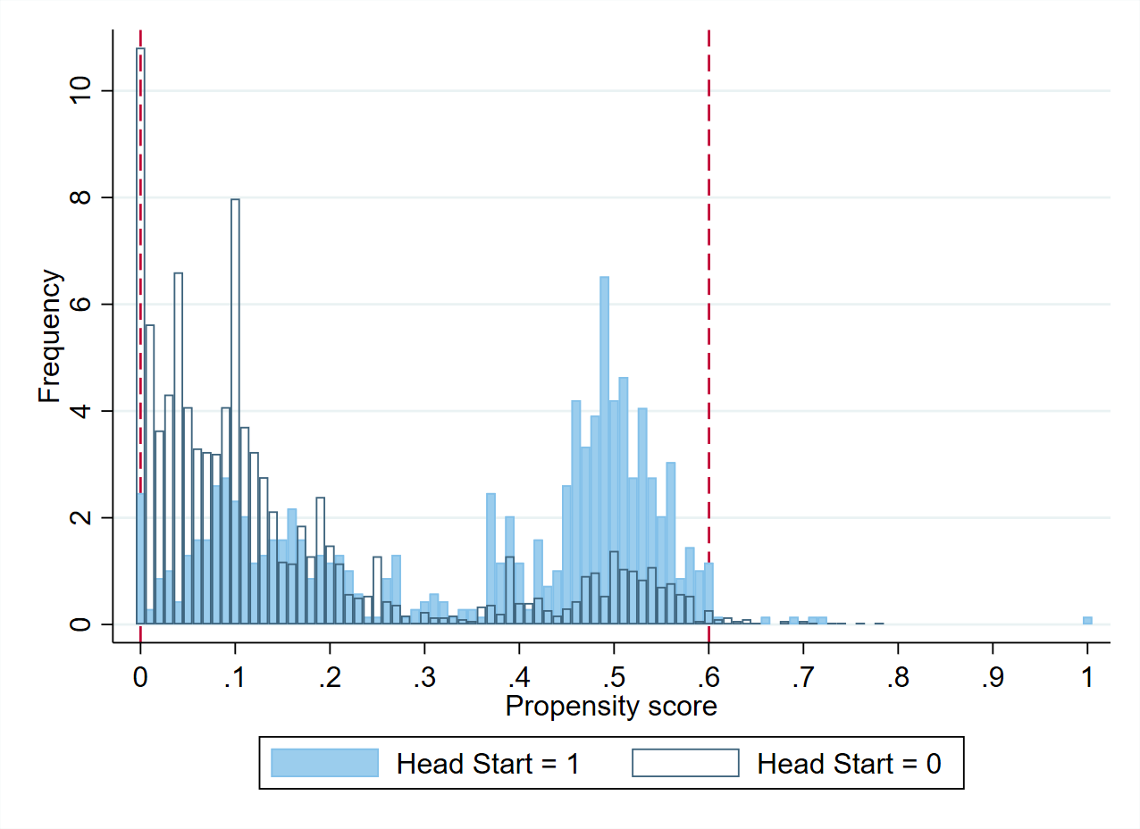
In the first step, we nonparametrically regress the treatment variable (Head Start) on the covariates to generate propensity scores for the sample, by employing the kernel estimation method in (8) and (9) with the rule-of-thumb bandwidth. Figure 1 plots the frequency distribution of the estimated propensity score by treatment status. The figure shows that the propensity score in our sample follows a bimodal distribution, with the main peak being at approximately 0.5 for the participants and approximately 0.1 for the nonparticipants. To reduce the potential impact of outliers, we trim the observations of the 1% smallest and 1% largest propensity scores in the second-step estimation. This trimming leads to a common support ranging from 0 to 0.6, as indicated by the two dashed vertical lines.

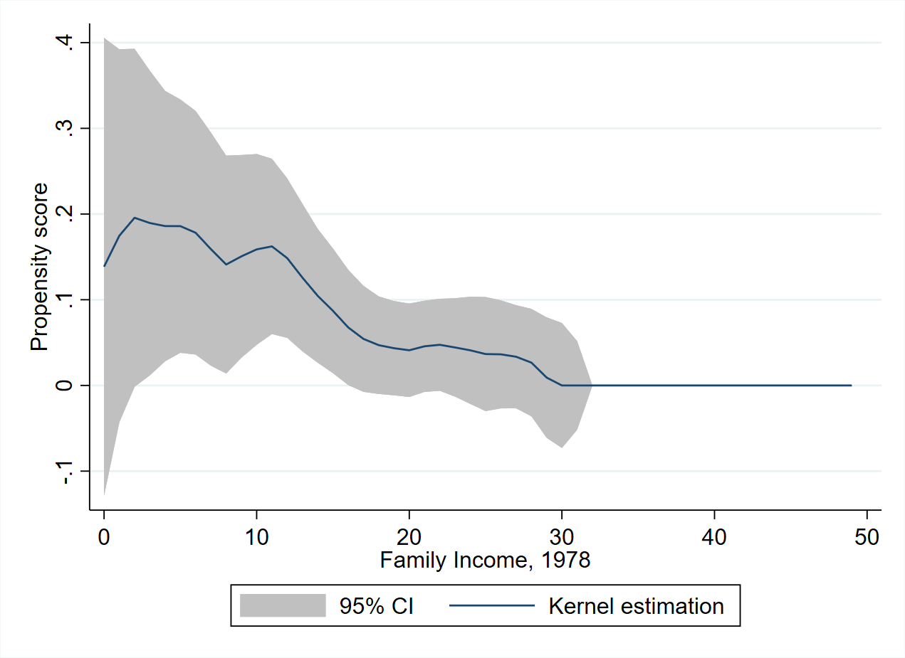
Note that only one continuous covariate exists in our data, that is, family income in 1978. Thus, we invoke Assumption NL1, which requires the propensity score to be a nonmonotonic function of the continuous covariate, given certain values of the discrete covariates. To verify Assumption NL1, we estimate the propensity score as a univariate function of family income in 1978 by using the largest data cell (32 years old, male, white race, parental education being high school or lower), with 175 observations, and plot it in Figure 2. We find that though low family income is an important eligibility criterion for enrollment in Head Start, the probability of participation is not simply a monotonically decreasing function of family income, possibly owing to the parents’ self-selection. Hence, Assumption NL1 is fulfilled.

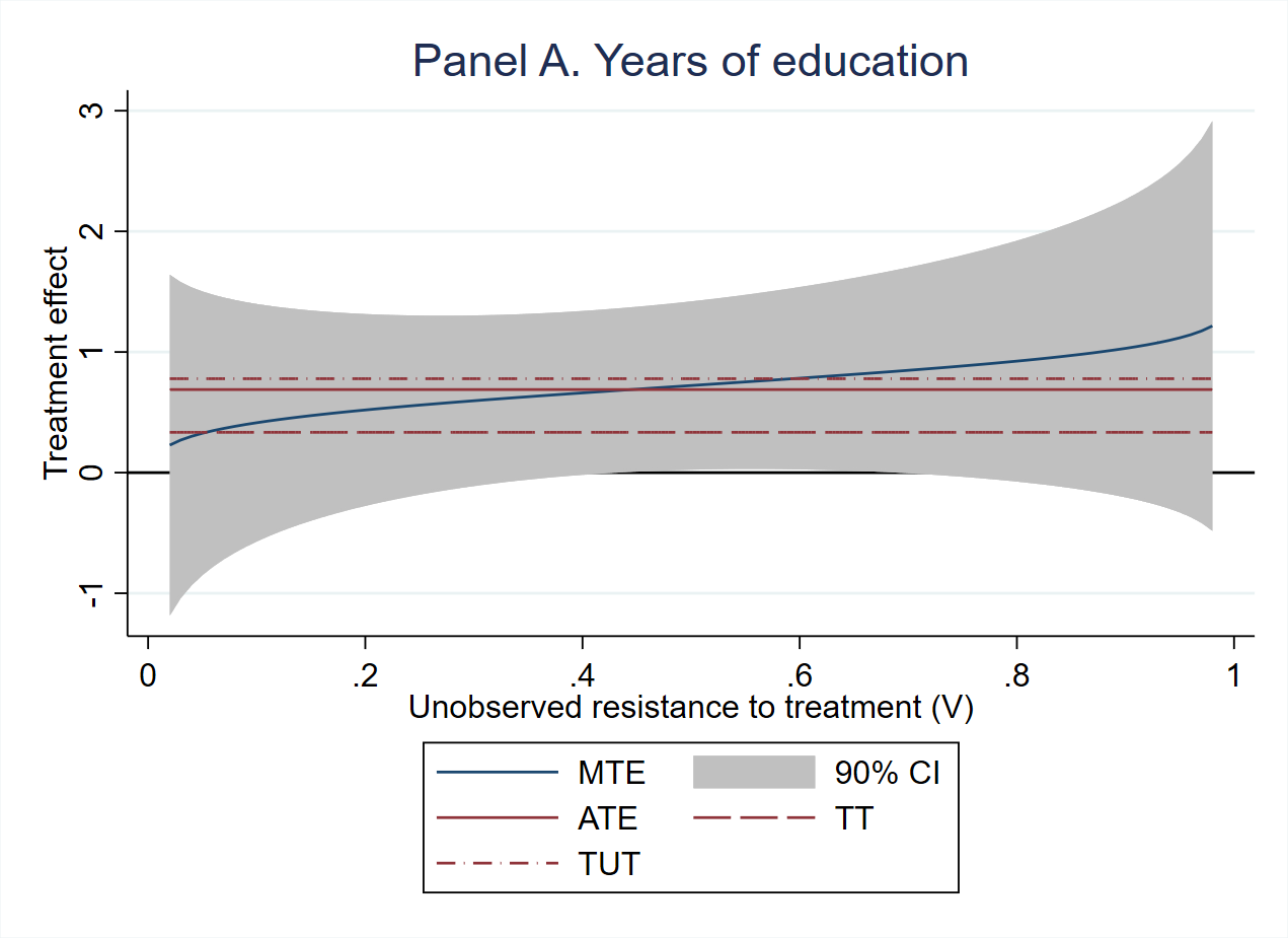
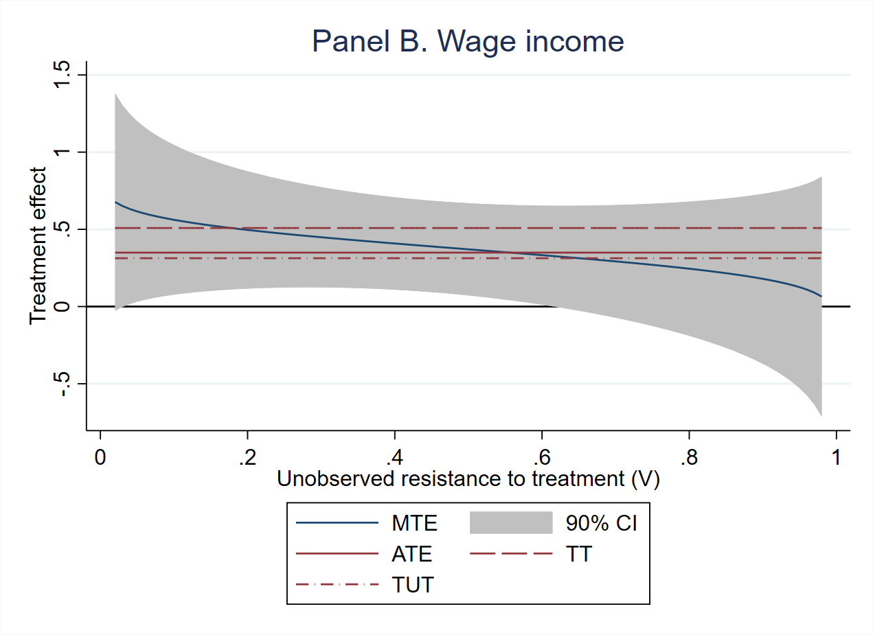
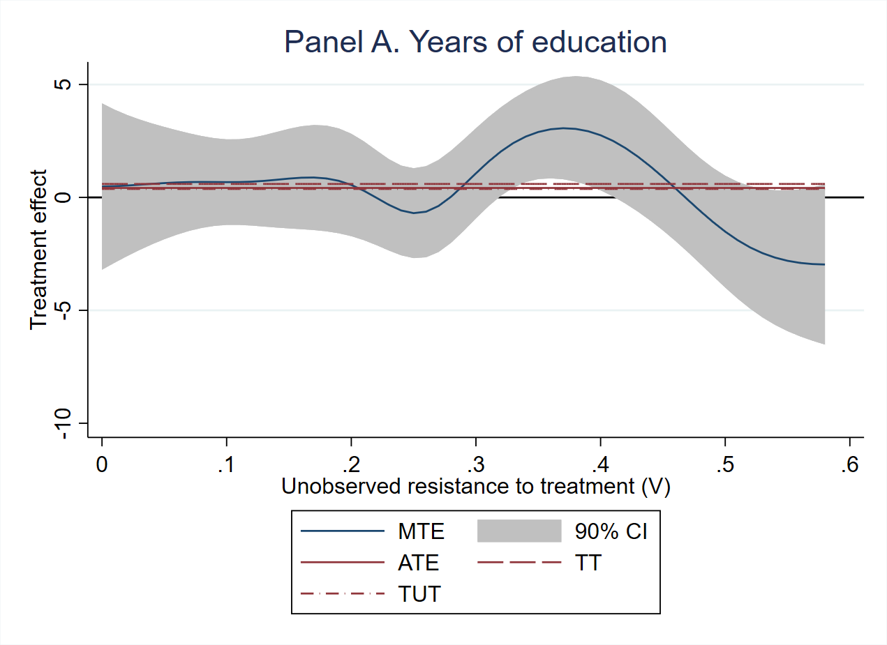
Given the estimated propensity score, we then estimate the MTE and summary treatment effect measures, such as the ATE, TT, and TUT, in the second step. We adopt the separate estimation procedure, since it generally exploits more identifying information behind the data than the LIV procedure (Brinch et al., 2017). Figure 3 shows the estimation results under Heckman’s normal specification that $E\left[\left.U_{d}\right|V=v\right]=\rho_{d}\Phi^{-1}\left(v\right)$ for $d=0,1$, where $\Phi\left(\cdot\right)$ is the CDF of the normal distribution, which can be derived by assuming that $\left(U_{d},V\right)$ follows a bivariate normal distribution with covariance $\rho_{d}$. The MTE curves, evaluated at the mean values of $X$, relate the unobserved component $U_{1}-U_{0}$ of the treatment effect to the unobserved component $V$ of the treatment choice. A high value of $V$ implies a low probability of treatment; thus, we interpret $V$ as resistance to participation in Head Start. The MTE curve for wage income plotted in panel B decreases with resistance, revealing a pattern of selection on gains, as expected. In other words, based on the unobserved characteristics, the children who were most likely to enroll in Head Start benefitted the most from the program in terms of their labor market outcome. However, when the outcome is educational attainment in panel A, the positive slope of the MTE curve points to a pattern of reverse selection on gains. As a consequence, the TUT exceeds the ATE, which in turn exceeds the TT. The same pattern was observed by Cornelissen et al. (2018) when estimating school-readiness return to a preschool program in Germany. This phenomenon may be attributed partly to the fact that parents have their own objectives in deciding childcare arrangements. Nevertheless, the disagreement between selection patterns for the two outcomes raises concern about the possible functional form misspecification of the normal MTE, which is strictly restricted to be monotonic in the resistance to treatment. Therefore, we consider a nonparametric specification for $E\left[\left.U_{d}\right|V=v\right]$ and implement a semiparametric separate estimation procedure.

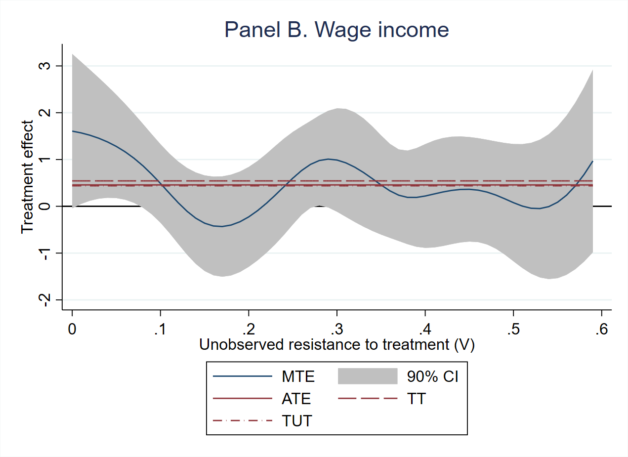
Figure 4 plots the semiparametric MTE curves for education and labor market outcomes in panels A and B, respectively. Under the flexible specification, the MTE curves are no longer monotonic, and the clear pattern of selection disappears. In the case of education outcome, the curve is initially flat, then becomes an inverted U shape, with a statistically significant positive effect appearing in the region of the peak, corresponding to the children with resistance to treatment ranging from 0.32 to 0.42. The complex feature of this curve is hardly captured by any parsimonious parametric function. Similar observations are seen in the case of wage income, in which the MTE curve is nonmonotonic, with a complex shape, and significantly greater than zero for less than 10% of the children who were most likely to attend childcare early. A comparison of the summary treatment effect measures indicates weak selection on gains for both outcomes. Table 1 reports the semiparametric estimates for the effects of the covariates on potential outcomes and their difference based on (10). Columns 3 and 6 show that girls gain significantly more returns to Head Start attendance than boys. However, other than gender, no substantial observable heterogeneity exists in the treatment effects of the program, though parental education and family income in 1978 have a significantly positive effect on the respondents’ potential education and potential labor market outcomes in both the treated and untreated states.

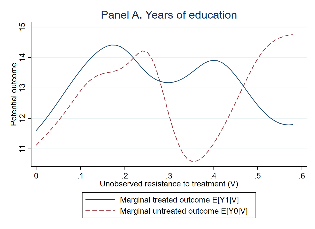
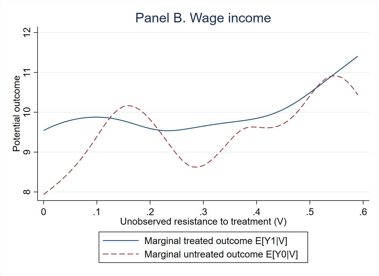
Based on $\hat{\beta}_{1}$ and $\hat{\beta}_{0}$ reported in Table 1, and the separate estimates of $E\left[\left.U_{d}\right|V=v\right]$ for $d=0,1$ under the semiparametric specification, we estimate the marginal structural functions

$$E\left[\left.Y_{d}\right|V=v\right]=E\left[X\right]^{\prime}\beta_{d}+E\left[\left.U_{d}\right|V=v\right]$$

for potential outcomes $Y_{1}$ and $Y_{0}$, which we plot in Figure 5. Panel A sheds light on the significantly positive effect of Head Start on education for the respondents with medium-level resistance to treatment, revealing that their gains from the program are driven mainly by the remarkably low educational attainment when untreated. Panel B leads to similar results for wage income, where significant gain emerges for low values of $V$. Moreover, the relatively flat curve of potential wage income in the treated state implies that early childcare attendance serves as an equalizer that diminishes the intergroup difference in the labor market outcome.

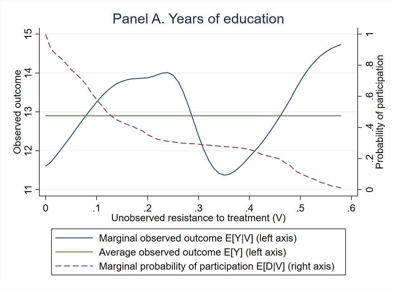
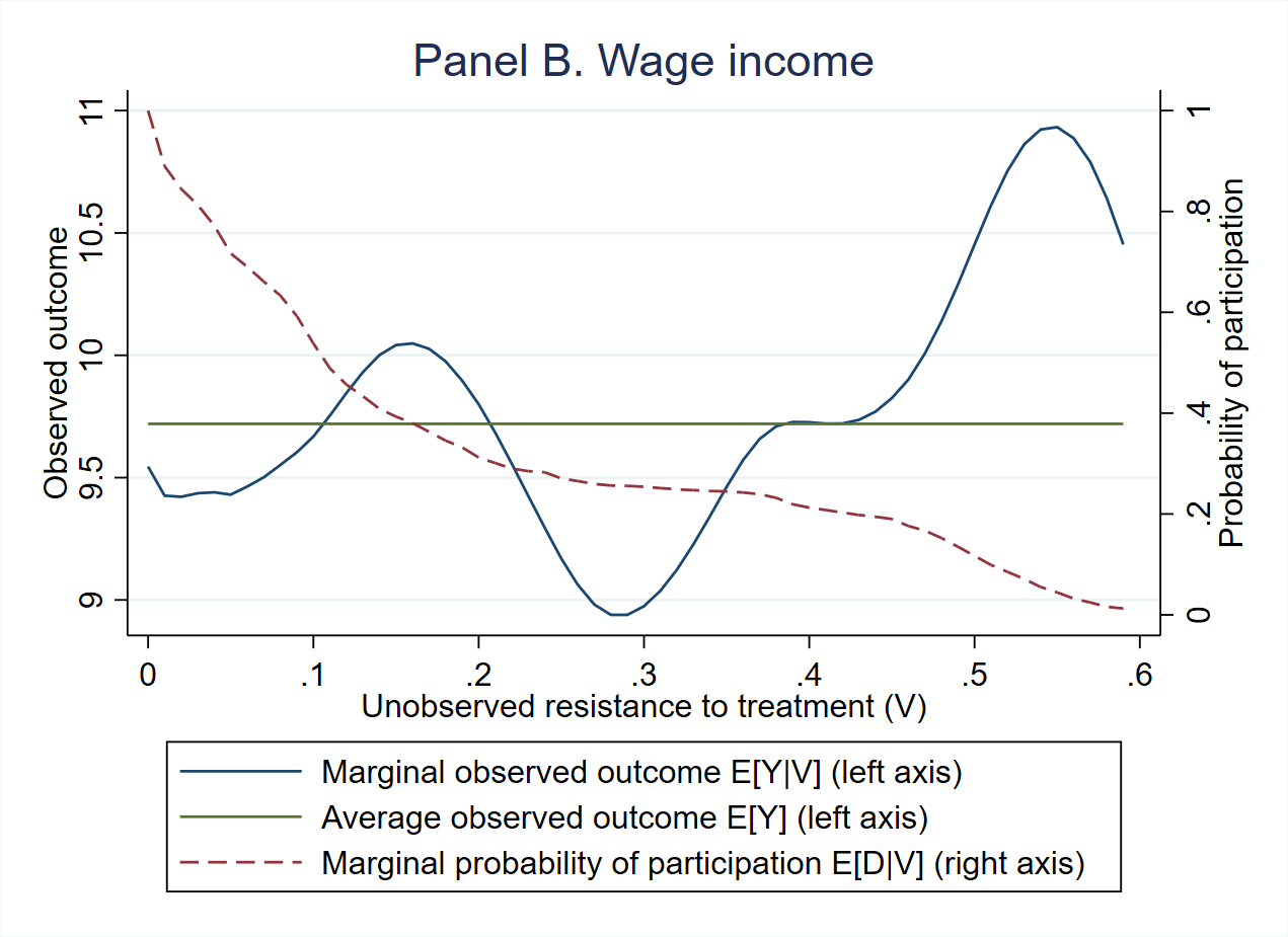
In addition, we can semiparametrically estimate conditional expectations of the observed responses given the unobserved determinants of treatment choice, such as the marginal probability of participation

$$E\left[\left.D\right|V=v\right]=\Pr\left(\left.P\geq v\right|V=v\right)=\Pr\left(P\geq v\right),$$

which mirrors the distribution of the propensity score, and the marginal observed outcome

$$E\left[\left.Y\right|V=v\right] = E\left[\left.Y_{0}\right|V=v\right]+E\left[\left.D\left(Y_{1}-Y_{0}\right)\right|V=v\right]$$

$$= E\left[\left.Y_{0}\right|V=v\right]+E\left[\left.DX\right|V=v\right]^{\prime}\left(\beta_{1}-\beta_{0}\right)+E\left[\left.D\left(U_{1}-U_{0}\right)\right|V=v\right]$$

$$= E\left[\left.Y_{0}\right|V=v\right]+E\left[1\left\{P\geq v\right\}X\right]^{\prime}\left(\beta_{1}-\beta_{0}\right)+\Pr\left(P\geq v\right)\cdot E\left[\left.U_{1}-U_{0}\right|V=v\right],$$

where the last equality follows from the independence of $X$ and $V$ and from the conditional mean independence of $X$ and $U_{d}$ given $V$. Plugging in proper estimates of each component in the above equations, we obtain the estimated marginal response functions and plot them in Figure 6. In particular, the marginal observed outcome curves relate the individuals with significant positive returns (with medium $V$ in Panel A and small $V$ in Panel B) to those with low education and low wage income, thereby bridging our findings on the MTE and those of De Haan and Leuven (2020) on the distributional treatment effect.

6 Conclusion

We propose a novel method for defining, identifying, and estimating the MTE in the absence of IVs. Our MTE model allows all the covariates to be correlated to the structural treatment error and does not require IVs. In this model, we define the MTE based on a reduced-form treatment error that (i) is uniformly distributed on the unit interval, (ii) is statistically independent of all the covariates, and (iii) has several economic meanings. The independence property facilitates the identification of our defined MTE. We provide sufficient conditions under which the MTE can be point identified based on functional form. The conditions are standard in a certain sense. The linearity and nonlinearity assumptions are the foundation of identification based on functional form, and can make sense to most empirical studies. The conditional mean independence assumption is equivalent to the separability assumption commonly imposed in the MTE literature, and is implied by and much weaker than the full independence assumption. We prove the identification by using a construction method. Our identification strategy allows the adaptation of most of the existing estimation procedures for conventional IV-MTE models, such as separate estimation, local IV estimation, parametric estimation, and semiparametric estimation. For the empirical application, we evaluate the MTE of the Head Start program on long-term education and labor market outcomes, in which an IV for Head Start participation is difficult to acquire. We find significant positive effects for the individuals with medium-level or low resistance to treatment, but substantial heterogeneity exists.

Figures and tables

Figure 1: Common Support. The figure plots the frequency distribution of the propensity score by treatment status. The propensity score is predicted via nonparametric kernel regression estimation. The dashed reference lines indicate the lower limit (0) and upper limit (0.6) of the propensity score with common support (based on 1% trimming on both sides).

Figure 2: Informal Test for Assumption NL1. The figure plots the propensity score as a function of family income in 1978, which is the only included continuous covariates in our data. The function is nonparametrically estimated using the largest data cell, with 175 observations. The nonmonotonicity of this estimated function validates Assumption NL1.

Figure 3: MTE Curves under Normal Specification. The MTE is estimated by the separate procedure based on parametric normal specification and evaluated at mean values of the covariates. Panels A and B depict the estimated MTE curves for education outcome and labor market outcome, respectively. The 90% confidence interval is based on bootstrapping with 1,000 replications.

Figure 4: MTE Curves under Semiparametric Specification. The MTE is estimated by the separate procedure based on the semiparametric specification, with the rule-of-thumb bandwidth, and evaluated at the mean values of the covariates. Panels A and B depict the estimated MTE curves for education outcome and labor market outcome, respectively. The 90% confidence interval is based on bootstrapping with 1,000 replications.

Figure 5: Semiparametric Estimates of Marginal Structural Functions. The marginal structural function refers to the expected potential outcome conditional on the unobserved resistance to treatment. Panels A and B depict the estimated marginal structural function curves for education outcome and labor market outcome, respectively. The 90% confidence interval is based on bootstrapping with 1,000 replications.

Figure 6: Semiparametric Estimates of Marginal Response Functions. This figure plots the (conditional) expectation of the observed outcome (solid line on the left y-axis), and the conditional probability of participation (dashed line on the right y-axis). Panels A and B illustrate the estimated marginal response function curves for education outcome and labor market outcome, respectively. The 90% confidence interval is based on bootstrapping with 1,000 replications.

Table 1: Semiparametric estimates of outcome equation coefficients

	Years of education				Wage income
	Treated	Untreated	Difference		Treated	Untreated	Difference
	(1)	(2)	(3)		(4)	(5)	(6)
Age	0.000	0.000	0.000		0.005	0.007	-0.002
	(0.056)	(0.027)	(0.062)		(0.030)	(0.014)	(0.033)
Female	0.558∗∗∗	0.254∗∗∗	0.304∗		-0.321∗∗∗	-0.503∗∗∗	0.182∗∗
	(0.159)	(0.078)	(0.174)		(0.083)	(0.039)	(0.091)
Black	-0.378	-0.226	-0.152		-0.015	-0.404∗∗∗	0.389
	(0.518)	(0.227)	(0.559)		(0.216)	(0.145)	(0.263)
Hispanic	-0.642	-0.403∗∗∗	-0.239		-0.097	-0.000	-0.097
	(0.408)	(0.145)	(0.430)		(0.169)	(0.068)	(0.183)
Parental education	1.764∗∗∗	1.796∗∗∗	-0.032		0.247∗∗	0.197∗∗∗	0.050
	(0.254)	(0.108)	(0.271)		(0.096)	(0.050)	(0.107)
Family income 1978	0.053∗∗∗	0.047∗∗∗	0.006		0.021∗∗∗	0.014∗∗∗	0.007
	(0.011)	(0.004)	(0.012)		(0.005)	(0.002)	(0.005)
ATE			0.421				0.457∗∗
			(0.492)				(0.228)
TT			0.597				0.543
			(1.047)				(0.484)
TUT			0.376				0.438∗
			(0.579)				(0.266)
Sample size	4,554				3,589

Notes: Columns 1 and 4 display the estimates of coefficients in the treated state ($\beta_{1}$ in Equation [6]), and columns 2 and 5 display the estimates of coefficients in the untreated state ($\beta_{0}$). Columns 3 and 6 display the difference in the estimates between the treated and untreated states ($\beta_{1}-\beta_{0}$), as well as the summary causal parameters (i.e., ATE, TT, and TUT). Bootstrapped standard errors from 1,000 replications are reported in parentheses.
^∗ Significant at the 10% level
^∗∗ Significant at the 5% level
^∗∗∗ Significant at the 1% level

Appendix

A.1 Proof of Theorem 1

Denote $m_{d}\left(x\right)=E\left[Y\left|X=x,D=d\right.\right]$ and $m_{d0}\left(x^{C}\right)=m_{d}\left(x^{C},0\right)$, $d=0,1$. Note that $\pi\left(x\right)$ and $m_{d}\left(x\right)$, and thus $\pi_{0}\left(x^{C}\right)$ and $m_{d0}\left(x^{C}\right)$, are identified functions because they are conditional expectations of observed variables. We first consider identifying $\beta_{d}^{C}$, the coefficients of continuous covariates, from $\pi_{0}\left(x^{C}\right)$ and $m_{d0}\left(x^{C}\right)$. By equation (5), we have

$$m_{d0}\left(x^{C}\right)=x^{C\prime}\beta_{d}^{C}+g_{d}\left(\pi_{0}\left(x^{C}\right)\right).$$ (A.1)

When $\dim\left(X^{C}\right)=1$, Assumption NL1 implies that

$$m_{d0}\left(x^{C}\right)-x^{C}\beta_{d}^{C}=g_{d}\left(\pi_{0}\left(x^{C}\right)\right)=g_{d}\left(\pi_{0}\left(\tilde{x}^{C}\right)\right)=m_{d0}\left(\tilde{x}^{C}\right)-\tilde{x}^{C}\beta_{d}^{C}.$$

Hence, $\beta_{d}^{C}$ is identified as

$$\beta_{d}^{C}=\frac{m_{d0}\left(x^{C}\right)-m_{d0}\left(\tilde{x}^{C}\right)}{x^{C}-\tilde{x}^{C}}.$$

When $\dim\left(X^{C}\right)\geq 2$, for $k,j\in\left\{1,2,\cdots,\dim\left(X^{C}\right)\right\}$ satisfying Assumption NL2, taking the partial derivatives of $m_{d0}\left(x^{C}\right)$ with respect to $x_{k}^{C}$ and $x_{j}^{C}$ yields that

$$\partial_{k}m_{d0}\left(x^{C}\right) = \beta_{d,k}^{C}+g_{d}^{\left(1\right)}\left(\pi_{0}\left(x^{C}\right)\right)\partial_{k}\pi_{0}\left(x^{C}\right),$$

$$\partial_{j}m_{d0}\left(x^{C}\right) = \beta_{d,j}^{C}+g_{d}^{\left(1\right)}\left(\pi_{0}\left(x^{C}\right)\right)\partial_{j}\pi_{0}\left(x^{C}\right).$$

It follows from Assumption NL2 (i)-(ii) that

$$\frac{\partial_{k}m_{d0}\left(x^{C}\right)-\beta_{d,k}^{C}}{\partial_{k}\pi_{0}\left(x^{C}\right)}=g_{d}^{\left(1\right)}\left(\pi_{0}\left(x^{C}\right)\right)=\frac{\partial_{j}m_{d0}\left(x^{C}\right)-\beta_{d,j}^{C}}{\partial_{j}\pi_{0}\left(x^{C}\right)},$$

so that

$$\partial_{k}m_{d0}\left(x^{C}\right)\partial_{j}\pi_{0}\left(x^{C}\right)-\partial_{j}m_{d0}\left(x^{C}\right)\partial_{k}\pi_{0}\left(x^{C}\right)=\partial_{j}\pi_{0}\left(x^{C}\right)\beta_{d,k}^{C}-\partial_{k}\pi_{0}\left(x^{C}\right)\beta_{d,j}^{C},$$ (A.2)

which is linear in $\beta_{d,k}^{C}$ and $\beta_{d,j}^{C}$. The same equation is obtained if we evaluate the expression at another point $\tilde{x}^{C}$ that satisfies Assumption NL2 (iii)-(iv), which gives

$$\left(\begin{array}[]{c}\partial_{k}m_{d0}\left(x^{C}\right)\partial_{j}\pi_{0}\left(x^{C}\right)-\partial_{j}m_{d0}\left(x^{C}\right)\partial_{k}\pi_{0}\left(x^{C}\right)\\ \partial_{k}m_{d0}\left(\tilde{x}^{C}\right)\partial_{j}\pi_{0}\left(\tilde{x}^{C}\right)-\partial_{j}m_{d0}\left(\tilde{x}^{C}\right)\partial_{k}\pi_{0}\left(\tilde{x}^{C}\right)\end{array}\right)=\Psi\left(\begin{array}[]{c}\beta_{d,k}^{C}\\ \beta_{d,j}^{C}\end{array}\right),$$ (A.3)

where

$$\Psi=\left(\begin{array}[]{cc}\partial_{j}\pi_{0}\left(x^{C}\right)&-\partial_{k}\pi_{0}\left(x^{C}\right)\\ \partial_{j}\pi_{0}\left(\tilde{x}^{C}\right)&-\partial_{k}\pi_{0}\left(\tilde{x}^{C}\right)\end{array}\right).$$

Assumption NL2 (v) ensures that the determinant of $\Psi$ is nonzero, which shows that $\Psi$ is nonsingular. Therefore, equation (A.3) can be solved for $\beta_{d,k}^{C}$ and $\beta_{d,j}^{C}$ by inverting $\Psi$, thereby identifying $\beta_{d,k}^{C}$ and $\beta_{d,j}^{C}$. Given identification of $\beta_{d,k}^{C}$, we can then identify all other coefficient $\beta_{d,l}^{C}$ in $\beta_{d}^{C}$ by solving (A.2) with the subscript $j$ replaced by $l$, which gives

$$\beta_{d,l}^{C}=\frac{\partial_{l}m_{d0}\left(x^{C}\right)\partial_{k}\pi_{0}\left(x^{C}\right)-\partial_{k}m_{d0}\left(x^{C}\right)\partial_{l}\pi_{0}\left(x^{C}\right)+\partial_{l}\pi_{0}\left(x^{C}\right)\beta_{d,k}^{C}}{\partial_{k}\pi_{0}\left(x^{C}\right)}.$$

Given the identification of $\beta_{d}^{C}$, the function $g_{d}$ is identified on the support of $\pi_{0}\left(X^{C}\right)$ by

$$g_{d}\left(p\right)=E\left[\left.m_{d0}\left(X^{C}\right)-X^{C\prime}\beta_{d}^{C}\right|\pi_{0}\left(X^{C}\right)=p\right].$$

Next, we consider identifying $\beta_{d}^{D}$, the coefficients of discrete covariates. For each $k\in\left\{1,2,\cdots,\dim\left(X^{D}\right)\right\}$, we have

$$m_{d}\left(x^{C},x^{Dk}\right)=x^{C\prime}\beta_{d}^{C}+x_{k}^{D}\beta_{d,k}^{D}+g_{d}\left(\pi\left(x^{C},x^{Dk}\right)\right)$$

for any $x^{C}$ in the support of $X^{C}$. By Assumption S, there exists $x^{C}\left(k\right)$ in the support of $X^{C}$ such that $\pi\left(x^{C}\left(k\right),x^{Dk}\right)$ is in the support of $\pi_{0}\left(X^{C}\right)$. It follows from the above identification result that $g_{d}\left(\pi\left(x^{C}\left(k\right),x^{Dk}\right)\right)$ is identified. Consequently, $\beta_{d,k}^{D}$ is identified by

$$\beta_{d,k}^{D}=\frac{m_{d}\left(x^{C}\left(k\right),x^{Dk}\right)-x^{C}\left(k\right)^{\prime}\beta_{d}^{C}-g_{d}\left(\pi\left(x^{C}\left(k\right),x^{Dk}\right)\right)}{x_{k}^{D}}.$$

This argument holds for each $k\in\left\{1,2,\cdots,\dim\left(X^{D}\right)\right\}$, thereby identifying $\beta_{d}^{D}$. Finally, given the identification of $\beta_{d}=\left(\beta_{d}^{C},\beta_{d}^{D}\right)$, it follows from (5) that the function $g_{d}$ is identified on the support of $P=\pi\left(X\right)$ by

$$g_{d}\left(p\right)=E\left[\left.m_{d}\left(X\right)-X^{\prime}\beta_{d}\right|\pi\left(X\right)=p\right],$$

for $d=0,1$.

A.2 Further discussion on the nonlinearity assumption

In light of the proof of Theorem 1, the local irrelevance assumption NL1 can be replaced by a differential version when there is only one continuous covariate, as given in the following theorem.

Theorem A.1.

Theorem 1 holds if Assumption NL1 is replaced by that a constant $x^{C}$ exists in the support of $X^{C}$ such that functions $\pi_{0}$ and $m_{d0}$ are differentiable at $x^{C}$ and $\left.\pi_{0}^{\left(1\right)}\left(x^{C}\right)=d\pi_{0}\left(x^{C}\right)\right/dx^{C}=0$.

Proof.

When $\dim\left(X^{C}\right)=1$, taking the derivative of both sides of (A.1) and evaluating at $x^{C}$, we obtain

$$m_{d0}^{\left(1\right)}\left(x^{C}\right)=\beta_{d}^{C}+g_{d}^{\left(1\right)}\left(\pi_{0}\left(x^{C}\right)\right)\pi_{0}^{\left(1\right)}\left(x^{C}\right)=\beta_{d}^{C},$$

which identifies $\beta_{d}^{C}$ for $d=0,1$. The remaining part of the proof is the same as the proof of Theorem 1.    

Compared with Assumption NL1, the condition of Theorem A.1 may be satisfied even if $\pi_{0}\left(x^{C}\right)$ is a strictly monotonic function as long as it has a stationary point, such as $\pi_{0}\left(x^{C}\right)=\left(x^{C}\right)^{3}$ at $x^{C}=0$. The two theorems below show that the local irrelevance condition can be extended to the case of multiple continuous covariates.

Theorem A.2.

Theorem 1 holds if Assumption NL is replaced by that (i) there are two points $x^{C}$ and $\tilde{x}^{C}$ in the support of $X^{C}$ and an index $k$ such that $x_{k}^{C}\neq\tilde{x}_{k}^{C}$, $x_{-k}^{C}=\tilde{x}_{-k}^{C}$, and $\pi_{0}\left(x^{C}\right)=\pi_{0}\left(\tilde{x}^{C}\right)$, and (ii) there exists $\breve{x}^{C}$ in the support of $X^{C}$ such that functions $\pi_{0}$ and $m_{d0}$ are differentiable at $\breve{x}^{C}$, with $\partial_{k}\pi_{0}\left(\breve{x}^{C}\right)\neq 0$.

Proof.

It follows from equation (A.1) and $\pi_{0}\left(x^{C}\right)=\pi_{0}\left(\tilde{x}^{C}\right)$ that

$$m_{d0}\left(x^{C}\right)-x_{k}^{C}\beta_{d,k}^{C}-x_{-k}^{C\prime}\beta_{d,-k}^{C}=m_{d0}\left(\tilde{x}^{C}\right)-\tilde{x}_{k}^{C}\beta_{d,k}^{C}-\tilde{x}_{-k}^{C^{\prime}}\beta_{d,-k}^{C}.$$

Hence, $\beta_{d,k}^{C}$ is identified by condition (i) as

$$\beta_{d,k}^{C}=\frac{m_{d0}\left(x^{C}\right)-m_{d0}\left(\tilde{x}^{C}\right)}{x_{k}^{C}-\tilde{x}_{k}^{C}}.$$

For any index $j\neq k$, taking the partial derivatives of $m_{d0}\left(x^{C}\right)$ with respect to $x_{k}^{C}$ and $x_{j}^{C}$ at $\breve{x}^{C}$ yields that

$$\partial_{k}m_{d0}\left(\breve{x}^{C}\right) = \beta_{d,k}^{C}+g_{d}^{\left(1\right)}\left(\pi_{0}\left(\breve{x}^{C}\right)\right)\partial_{k}\pi_{0}\left(\breve{x}^{C}\right),$$ (A.4)

$$\partial_{j}m_{d0}\left(\breve{x}^{C}\right) = \beta_{d,j}^{C}+g_{d}^{\left(1\right)}\left(\pi_{0}\left(\breve{x}^{C}\right)\right)\partial_{j}\pi_{0}\left(\breve{x}^{C}\right).$$ (A.5)

Since $\partial_{k}\pi_{0}\left(\breve{x}^{C}\right)\neq 0$ by condition (ii), we can find $g_{d}^{\left(1\right)}\left(\pi_{0}\left(\breve{x}^{C}\right)\right)$ from (A.4) to be

$$g_{d}^{\left(1\right)}\left(\pi_{0}\left(\breve{x}^{C}\right)\right)=\frac{\partial_{k}m_{d0}\left(\breve{x}^{C}\right)-\beta_{d,k}^{C}}{\partial_{k}\pi_{0}\left(\breve{x}^{C}\right)},$$

and substitute it into (A.5) to identify $\beta_{d,j}^{C}$ as

$$\beta_{d,j}^{C}=\partial_{j}m_{d0}\left(\breve{x}^{C}\right)-\frac{\partial_{j}\pi_{0}\left(\breve{x}^{C}\right)}{\partial_{k}\pi_{0}\left(\breve{x}^{C}\right)}\left[\partial_{k}m_{d0}\left(\breve{x}^{C}\right)-\beta_{d,k}^{C}\right].$$

Therefore, $\beta_{d}^{C}$ is identified. The remaining part of the proof is the same as the proof of Theorem 1.    

Theorem A.3.

Theorem 1 holds if Assumption NL is replaced by that there exist two points $x^{C}$ and $\tilde{x}^{C}$ in the support of $X^{C}$ and an index $k$ such that functions $\pi_{0}$ and $m_{d0}$ are differentiable at $x^{C}$ and $\tilde{x}^{C}$, with $\partial_{k}\pi_{0}\left(x^{C}\right)=0$ and $\partial_{k}\pi_{0}\left(\tilde{x}^{C}\right)\neq 0$.

Proof.

The identification of $\beta_{d,k}^{C}$ is analogous to Theorem A.1. Then, the identification of all the other coefficients $\beta_{d,j}^{C}$ in $\beta_{d}^{C}$ and the remaining components of the model is the same as in Theorem A.2 and Theorem 1, respectively.    

Alternatively, the identification of coefficients of continuous covariates can also be attained by exploiting the local irrelevance of the function $g_{d}\left(p\right)$.

Theorem A.4.

Theorem 1 holds if Assumption NL is replaced by that, there exists $x^{C}$ in the support of $X^{C}$ such that $g_{d}^{\left(1\right)}\left(\pi_{0}\left(x^{C}\right)\right)=0$ for $d=0,1$, and functions $\pi_{0}$ and $m_{d0}$ are differentiable at $x^{C}$.

Proof.

For each $k\in\left\{1,2,\cdots,\dim\left(X^{C}\right)\right\}$, taking the partial derivative of both sides of (A.1) with respect to $x_{k}^{C}$ gives

$$\partial_{k}m_{d0}\left(x^{C}\right)=\beta_{d,k}^{C}+g_{d}^{\left(1\right)}\left(\pi_{0}\left(x^{C}\right)\right)\partial_{k}\pi_{0}\left(x^{C}\right)=\beta_{d,k}^{C},$$

which immediately identifies all $\beta_{d,k}^{C}$ in $\beta_{d}^{C}$. The remaining part of the proof is the same as that of Theorem 1.    

The above discussion further illustrates the overidentification feature of our strategy. In fact, the identifying power of our method is determined by the number of nonlinearity points in the data satisfying Assumption NL or Theorems A.1-A.4.

A.3 Limited valued outcomes

To accommodate limited valued outcomes, we first generalize the linear additive model to a linear latent index model.

Assumption A.L (Linear index). Assume that $Y_{d}=l\left(X^{\prime}\gamma_{d},V_{d}\right)$, $d=0,1$, holds for some known link function $l$ and unknown coefficients $\gamma_{d}$, where $V_{d}$ is unobserved error term of $Y_{d}$.

The generalized linear model applies to a variety of frequently encountered limited dependent variables, such as $l\left(t,v\right)=1\left\{t\geq v\right\}$ for binary $Y\in\left\{0,1\right\}$, $l\left(t,v\right)=\max\left(t-v,0\right)$ for censored (at zero) $Y\geq 0$, $l\left(t,v\right)=\exp\left(t+v\right)\left/\left[1+\exp\left(t+v\right)\right]\right.$ for proportion-valued $Y\in\left(0,1\right)$, $l\left(t,v\right)=\sum_{j=1}^{s}1\left\{t+v\geq c_{j}\right\}$ for ordered $Y\in\left\{0,1,\cdots,s\right\}$ with known thresholds $c_{1}<c_{2}<\cdots<c_{s}$, and so forth. Although setting $l\left(t,v\right)=t+v$ reduces to the linear additive model, the following discussion does not include Theorem 1 as a special case because $\gamma_{d}$ here can be only identified up to scale for a general link function $l$. Any changes in the scaling of $\gamma_{d}$ can be freely absorbed into $l$, and a scale normalization is needed for identification of $\gamma_{d}$ and $l$.

Assumption A.N (Normalization). Decompose $X^{\prime}\gamma_{d}=X^{C\prime}\gamma_{d}^{C}+X^{D\prime}\gamma_{d}^{D}$, where $X^{C}$ and $X^{D}$ consist of covariates that are continuously and discretely distributed, respectively. Assume that $\gamma_{d,1}^{C}$, the first element of $\gamma_{d}^{C}$, equal to 1.

Assumption A.N imposes the convenient normalization that the first continuous covariate has a unit coefficient. This scaling of $\gamma_{d}$ is arbitrary and is innocuous because our focus is on the identification of MTE, which is a difference in the conditional expectations of $l\left(X^{\prime}\gamma_{d},V_{d}\right)$, rather than on separate identification of $\gamma_{d}$ and $l$. Since in the generalized linear model the potential outcomes are not necessarily additive in the error term, the mean independence assumption needs to be strengthened to a stricter distributional independence assumption.

Assumption A.CI (Conditional Independence). Assume that $\left.V_{d}\perp\!\!\!\!\perp X\right|V$ for $d=0,1$, namely, $V_{d}$ is independent of $X$ conditional on $V$, where $V$ is the reduced-form treatment error in equation (3).

Recalling that $V\perp\!\!\!\!\perp X$ by definition, Assumption A.CI is equivalent to the full independence $\left(V_{d},V\right)\perp\!\!\!\!\perp X$ for $d=0,1$, which implies that both the marginal distribution of $V_{d}$ and the copula of $V_{d}$ and $V$ are independent of $X$. Under Assumptions A.L and A.CI, we have

$$\Delta^{\text{MTE}}\left(x,v\right)=E\left[\left.l\left(x^{\prime}\gamma_{1},V_{1}\right)-l\left(x^{\prime}\gamma_{0},V_{0}\right)\right|V=v\right].$$

The additive nonseparability of the observables and unobservables constitutes the primary difficulty in identifying MTE in the limited outcome case. Meanwhile, Assumptions A.L and A.CI lead to a double index form of the observable outcome regression functions for each treatment status, that is,

$$E\left[\left.Y1\left\{D=d\right\}\right|X=x\right]=r_{d}\left(x^{\prime}\gamma_{d},\pi\left(x\right)\right)$$ (A.6)

for $d=0,1$, where

$$r_{0}\left(t,p\right) = \int_{p}^{1}E\left[\left.l\left(t,V_{0}\right)\right|V=v\right]dv,$$ (A.7)

$$r_{1}\left(t,p\right) = \int_{0}^{p}E\left[\left.l\left(t,V_{1}\right)\right|V=v\right]dv.$$ (A.8)

Provided that $\pi\left(x\right)$ is a nonlinear index, $\gamma_{d}$ and thus $r_{d}$ can be identified based on functional form, which ensures identification of MTE since

$$\Delta^{\text{MTE}}\left(x,v\right)=\partial_{2}r_{1}\left(x^{\prime}\gamma_{1},v\right)+\partial_{2}r_{0}\left(x^{\prime}\gamma_{0},v\right),$$ (A.9)

where $\partial_{2}r_{d}$ is the partial derivative of $r_{d}$ with respect to its second argument. Like in the case of unlimited outcomes, the key powers of this identification strategy are supplied by the nonlinearity of $\pi\left(x\right)$, as specified by the following assumption.

Assumption A.NL (Non-Linearity). Assume that the functions $\pi_{0}$ and $r_{d}$ are differentiable and denote their partial derivatives with respect to the $k$-th argument as $\partial_{k}\pi_{0}$ and $\partial_{k}r_{d}$, where $\pi_{0}\left(x^{C}\right)=\pi\left(x^{C},0\right)$ and $r_{d}$, $d=0,1$, are defined in (A.6) and (A.6). Assume that there exist two vectors $x^{C}$ and $\tilde{x}^{C}$ on the support of $X^{C}$ and two elements $k$ and $j$ of the set $\left\{1,2,\cdots,\dim\left(X^{C}\right)\right\}$ such that (i) $\partial_{1}r_{d}\left(x^{C\prime}\gamma_{d}^{C},\pi_{0}\left(x^{C}\right)\right)\neq 0$, (ii) $\partial_{1}r_{d}\left(\tilde{x}^{C\prime}\gamma_{d}^{C},\pi_{0}\left(\tilde{x}^{C}\right)\right)\neq 0$, (iii) $\partial_{k}\pi_{0}\left(x^{C}\right)\neq\partial_{1}\pi_{0}\left(x^{C}\right)\gamma_{d,k}^{C}$, (iv) $\partial_{j}\pi_{0}\left(x^{C}\right)\neq\partial_{1}\pi_{0}\left(x^{C}\right)\gamma_{d,j}^{C}$, (v) $\partial_{l}\pi_{0}\left(\tilde{x}^{C}\right)\neq\partial_{1}\pi_{0}\left(\tilde{x}^{C}\right)\gamma_{d,l}^{C}$ for $l=2,\cdots,\dim\left(X^{C}\right)$, and

(vi) $$\partial_{k}\pi_{0}\left(x^{C}\right)\partial_{j}\pi_{0}\left(\tilde{x}^{C}\right)-\partial_{k}\pi_{0}\left(\tilde{x}^{C}\right)\partial_{j}\pi_{0}\left(x^{C}\right)$$

$$\neq \left[\partial_{1}\pi_{0}\left(x^{C}\right)\partial_{j}\pi_{0}\left(\tilde{x}^{C}\right)-\partial_{1}\pi_{0}\left(\tilde{x}^{C}\right)\partial_{j}\pi_{0}\left(x^{C}\right)\right]\gamma_{d,k}^{C}$$

$$-\left[\partial_{1}\pi_{0}\left(x^{C}\right)\partial_{k}\pi_{0}\left(\tilde{x}^{C}\right)-\partial_{1}\pi_{0}\left(\tilde{x}^{C}\right)\partial_{k}\pi_{0}\left(x^{C}\right)\right]\gamma_{d,j}^{C}.$$

Assumption A.NL (i)-(ii) require $r_{d}$ to depend on the linear index, and (iii)-(vi) essentially require some nonlinear variation in $\pi_{0}$ under the scale normalization. As in Assumption NL, it is difficult to construct examples other than $\pi_{0}\left(x^{C}\right)=f\left(x^{C\prime}\gamma\right)$ that violates Assumption A.NL. Finally, a support assumption and an invertibility assumption are imposed for technical reasons.

Assumption A.S (Support). For each $k\in\left\{1,2,\cdots,\dim\left(X^{D}\right)\right\}$, assume for some $x_{k}^{D}\neq 0$ in the support of $X_{k}^{D}$ that there exists $x^{C}\left(k\right)$ in the support of $X^{C}$ such that $\pi\left(x^{C}\left(k\right),x^{Dk}\right)$ is in the support of $\pi_{0}\left(X^{C}\right)$ and that $x^{C}\left(k\right)^{\prime}\gamma_{d}^{C}+x_{k}^{D}\gamma_{d,k}^{D}$ is in the support of $X^{C\prime}\gamma_{d}^{C}$ for $d=0,1$.

Assumption A.I (Invertibility). Assume that the function $r_{d}$ is invertible on its first argument for $d=0,1$.

For the case of a binary outcome, we have $r_{0}\left(t,p\right)=\int_{p}^{1}F_{\left.V_{0}\right|V}\left(\left.t\right|v\right)dv$ and $r_{1}\left(t,p\right)=\int_{0}^{p}F_{\left.V_{1}\right|V}\left(\left.t\right|v\right)dv$, hence a sufficient condition for Assumption A.I to hold is that $V_{d}$ is continuously distributed with support $\mathbb{R}$, conditional on $V$, for $d=0,1$. Interestingly, the same continuous distribution condition also suffices for Assumption A.I in the censored case with $l\left(t,v\right)=\max\left(t-v,0\right)$, where $\partial_{1}r_{0}\left(t,p\right)=\int_{p}^{1}F_{\left.V_{0}\right|V}\left(\left.t\right|v\right)dv$ and $\partial_{1}r_{1}\left(t,p\right)=\int_{0}^{p}F_{\left.V_{1}\right|V}\left(\left.t\right|v\right)dv$. Under the imposed assumptions, the following identification theorem for the generalized linear model follows immediately from Escanciano et al. (2016, Theorems 3.1-3.2).

Theorem A.5.

If Assumptions A.L, A.NL, A.CI, A.S, A.N, and A.I hold, then $\gamma_{d}$ and $r_{d}\left(t,p\right)$ at all points in the support of $X^{\prime}\gamma_{d}$ and $P$ are identified for $d=0,1$.

Having established identification of $\gamma_{d}$ and $r_{d}$, the MTE for limited valued outcomes can be identified by (A.9) and estimated by the semiparametric least squares method of Escanciano et al. (2016). Alternatively, the LIV estimation procedure may be adapted according to

$$E\left[\left.Y\right|X=x\right]=s\left(x^{\prime}\gamma_{0},x^{\prime}\gamma_{1},\pi\left(x\right)\right),$$

where

$$s\left(t_{0},t_{1},p\right)=r_{0}\left(t_{0},p\right)+r_{1}\left(t_{1},p\right),$$

and

$$\Delta^{\text{MTE}}\left(x,v\right) = \frac{\partial s\left(x^{\prime}\gamma_{0},x^{\prime}\gamma_{1},v\right)}{\partial v},$$

$$\Delta^{\text{ATE}}\left(x\right) = s\left(x^{\prime}\gamma_{0},x^{\prime}\gamma_{1},1\right)-s\left(x^{\prime}\gamma_{0},x^{\prime}\gamma_{1},0\right),$$

$$\Delta^{\text{TT}}\left(x\right) = \frac{s\left(x^{\prime}\gamma_{0},x^{\prime}\gamma_{1},\pi\left(x\right)\right)-s\left(x^{\prime}\gamma_{0},x^{\prime}\gamma_{1},0\right)}{\pi\left(x\right)},$$

$$\Delta^{\text{TUT}}\left(x\right) = \frac{s\left(x^{\prime}\gamma_{0},x^{\prime}\gamma_{1},1\right)-s\left(x^{\prime}\gamma_{0},x^{\prime}\gamma_{1},\pi\left(x\right)\right)}{1-\pi\left(x\right)},$$

$$\Delta^{\text{LATE}}\left(x,v_{1},v_{2}\right) = \frac{s\left(x^{\prime}\gamma_{0},x^{\prime}\gamma_{1},v_{2}\right)-s\left(x^{\prime}\gamma_{0},x^{\prime}\gamma_{1},v_{1}\right)}{v_{2}-v_{1}}.$$

References

- Ahn and Powell (1993) Ahn, H. and J. L. Powell (1993). Semiparametric estimation of censored selection models with a nonparametric selection mechanism. Journal of Econometrics 58(1-2), 3–29.
- Arnold et al. (2018) Arnold, D., W. Dobbie, and C. S. Yang (2018). Racial bias in bail decisions. The Quarterly Journal of Economics 133(4), 1885–1932.
- Aryal et al. (2022) Aryal, G., M. Bhuller, and F. Lange (2022). Signaling and employer learning with instruments. American Economic Review 112(5), 1669–1702.
- Barr and Gibbs (2022) Barr, A. and C. R. Gibbs (2022). Breaking the cycle? intergenerational effects of an antipoverty program in early childhood. Journal of Political Economy 130(12), 3253–3285.
- Bauer and Schanzenbach (2016) Bauer, L. and D. W. Schanzenbach (2016). The Long-Term Impact of the Head Start Program. Washington DC: Hamilton Project.
- Brinch et al. (2017) Brinch, C. N., M. Mogstad, and M. Wiswall (2017). Beyond LATE with a discrete instrument. Journal of Political Economy 125(4), 985–1039.
- Chamberlain (1986) Chamberlain, G. (1986). Asymptotic efficiency in semi-parametric models with censoring. Journal of Econometrics 32(2), 189–218.
- Conley et al. (2012) Conley, T. G., C. B. Hansen, and P. E. Rossi (2012). Plausibly exogenous. Review of Economics and Statistics 94(1), 260–272.
- Cornelissen et al. (2018) Cornelissen, T., C. Dustmann, A. Raute, and U. Schönberg (2018). Who benefits from universal child care? estimating marginal returns to early child care attendance. Journal of Political Economy 126(6), 2356–2409.
- Currie (2001) Currie, J. (2001). Early childhood education programs. Journal of Economic Perspectives 15(2), 213–238.
- De Haan and Leuven (2020) De Haan, M. and E. Leuven (2020). Head start and the distribution of long-term education and labor market outcomes. Journal of Labor Economics 38(3), 727–765.
- Deming (2009) Deming, D. (2009). Early childhood intervention and life-cycle skill development: Evidence from head start. American Economic Journal: Applied Economics 1(3), 111–134.
- D’Haultfœuille et al. (2021) D’Haultfœuille, X., S. Hoderlein, and Y. Sasaki (2021). Testing and relaxing the exclusion restriction in the control function approach. Journal of Econometrics (in press). Available at https://doi.org/10.1016/j.jeconom.2020.09.012.
- D’Haultfœuille and Maurel (2013) D’Haultfœuille, X. and A. Maurel (2013). Another look at the identification at infinity of sample selection models. Econometric Theory 29(1), 213–224.
- D’Haultfœuille et al. (2018) D’Haultfœuille, X., A. Maurel, and Y. Zhang (2018). Extremal quantile regressions for selection models and the black-white wage gap. Journal of Econometrics 203(1), 129–142.
- Dong (2010) Dong, Y. (2010). Endogenous regressor binary choice models without instruments, with an application to migration. Economics Letters 107(1), 33–35.
- Elango et al. (2016) Elango, S., J. L. García, J. J. Heckman, and A. Hojman (2016). Early childhood education. In R. A. Moffitt (Ed.), Economics of Means-Tested Transfer Programs in the United States, Volume 2. Chicago: University of Chicago Press.
- Escanciano et al. (2016) Escanciano, J. C., D. Jacho-Chávez, and A. Lewbel (2016). Identification and estimation of semiparametric two-step models. Quantitative Economics 7(2), 561–589.
- Fischer et al. (2020) Fischer, M., M. Karlsson, T. Nilsson, and N. Schwarz (2020). The long-term effects of long terms–compulsory schooling reforms in sweden. Journal of the European Economic Association 18(6), 2776–2823.
- Garces et al. (2002) Garces, E., D. Thomas, and J. Currie (2002). Longer-term effects of head start. American economic review 92(4), 999–1012.
- Garlick and Hyman (2022) Garlick, R. and J. Hyman (2022). Quasi-experimental evaluation of alternative sample selection corrections. Journal of Business & Economic Statistics 40(3), 950–964.
- Heckman (1979) Heckman, J. J. (1979). Sample selection bias as a specification error. Econometrica 47(1), 153–61.
- Heckman et al. (2018) Heckman, J. J., J. E. Humphries, and G. Veramendi (2018). Returns to education: The causal effects of education on earnings, health, and smoking. Journal of Political Economy 126(S1), S197–S246.
- Heckman and Vytlacil (1999) Heckman, J. J. and E. Vytlacil (1999). Local instrumental variables and latent variable models for identifying and bounding treatment effects. Proceedings of the national Academy of Sciences 96(8), 4730–4734.
- Heckman and Vytlacil (2001) Heckman, J. J. and E. Vytlacil (2001). Local instrumental variables. In C. Hsiao, K. Morimune, and J. L. Powell (Eds.), Nonlinear Statistical Modeling: Proceedings of the Thirteenth International Symposium in Economic Theory and Econometrics: Essays in Honor of Takeshi Amemiya, Chapter 1, pp. 1–46. Cambridge, U.K.: Cambridge University Press.
- Heckman and Vytlacil (2005) Heckman, J. J. and E. Vytlacil (2005). Structural equations, treatment effects, and econometric policy evaluation. Econometrica 73(3), 669–738.
- Honoré and Hu (2020) Honoré, B. E. and L. Hu (2020). Selection without exclusion. Econometrica 88(3), 1007–1029.
- Honoré and Hu (2022) Honoré, B. E. and L. Hu (2022). Sample selection models without exclusion restrictions: Parameter heterogeneity and partial identification. Journal of Econometrics (in press). Available at https://doi.org/10.1016/j.jeconom.2021.07.017.
- Ichimura (1993) Ichimura, H. (1993). Semiparametric least squares (SLS) and weighted SLS estimation of single-index models. Journal of Econometrics 58, 71–120.
- Jones (2015) Jones, D. (2015). The economics of exclusion restrictions in IV models. NBER Working Paper (No.21391). Available at https://doi.org/10.3386/w21391.
- Kamhöfer et al. (2019) Kamhöfer, D. A., H. Schmitz, and M. Westphal (2019). Heterogeneity in marginal non-monetary returns to higher education. Journal of the European Economic Association 17(1), 205–244.
- Kédagni and Mourifié (2020) Kédagni, D. and I. Mourifié (2020). Generalized instrumental inequalities: testing the instrumental variable independence assumption. Biometrika 107(3), 661–675.
- Khan and Tamer (2010) Khan, S. and E. Tamer (2010). Irregular identification, support conditions, and inverse weight estimation. Econometrica 78(6), 2021–2042.
- Kirkeboen et al. (2016) Kirkeboen, L. J., E. Leuven, and M. Mogstad (2016). Field of study, earnings, and self-selection. The Quarterly Journal of Economics 131(3), 1057–1111.
- Klein and Vella (2010) Klein, R. and F. Vella (2010). Estimating a class of triangular simultaneous equations models without exclusion restrictions. Journal of Econometrics 154(2), 154–164.
- Klein and Spady (1993) Klein, R. W. and R. H. Spady (1993). An efficient semiparametric estimator for binary response models. Econometrica 61, 387–421.
- Kline and Walters (2016) Kline, P. and C. R. Walters (2016). Evaluating public programs with close substitutes: The case of Head Start. The Quarterly Journal of Economics 131(4), 1795–1848.
- Lewbel (1997) Lewbel, A. (1997). Constructing instruments for regressions with measurement error when no additional data are available, with an ppplication to patents and r&d. Econometrica 65(5), 1201–1214.
- Lewbel (2000) Lewbel, A. (2000). Semiparametric qualitative response model estimation with unknown heteroscedasticity or instrumental variables. Journal of Econometrics 97(1), 145–177.
- Lewbel (2007) Lewbel, A. (2007). Endogenous selection or treatment model estimation. Journal of Econometrics 141(2), 777–806.
- Lewbel (2012) Lewbel, A. (2012). Using heteroscedasticity to identify and estimate mismeasured and endogenous regressor models. Journal of Business & Economic Statistics 30(1), 67–80.
- Lewbel (2018) Lewbel, A. (2018). Identification and estimation using heteroscedasticity without instruments: The binary endogenous regressor case. Economics Letters 165, 10–12.
- Lewbel (2019) Lewbel, A. (2019). The identification zoo: Meanings of identification in econometrics. Journal of Economic Literature 57(4), 835–903.
- Mogstad et al. (2018) Mogstad, M., A. Santos, and A. Torgovitsky (2018). Using instrumental variables for inference about policy relevant treatment parameters. Econometrica 86(5), 1589–1619.
- Mogstad et al. (2021) Mogstad, M., A. Torgovitsky, and C. R. Walters (2021). The causal interpretation of two-stage least squares with multiple instrumental variables. American Economic Review 111(11), 3663–98.
- Mountjoy (2022) Mountjoy, J. (2022). Community colleges and upward mobility. American Economic Review 112(8), 2580–2630.
- Mourifié et al. (2020) Mourifié, I., M. Henry, and R. Méango (2020). Sharp bounds and testability of a Roy model of STEM major choices. Journal of Political Economy 128(8), 3220–3283.
- Pan and Xie (2023) Pan, Z. and J. Xie (2023). -penalized pairwise difference estimation for a high-dimensional censored regression model. Journal of Business & Economic Statistics 41(2), 283–297.
- Pan et al. (2022) Pan, Z., X. Zhou, and Y. Zhou (2022). Semiparametric estimation of a censored regression model subject to nonparametric sample selection. Journal of Business & Economic Statistics 40(1), 141–151.
- Powell et al. (1989) Powell, J. L., J. H. Stock, and T. M. Stoker (1989). Semiparametric estimation of index coefficients. Econometrica 57(6), 1403–1430.
- Racine and Li (2004) Racine, J. and Q. Li (2004). Nonparametric estimation of regression functions with both categorical and continuous data. Journal of Econometrics 119(1), 99–130.
- Roy (1951) Roy, A. D. (1951). Some thoughts on the distribution of earnings. Oxford Economic Papers 3(2), 135–146.
- Rubin (1973a) Rubin, D. B. (1973a). Matching to remove bias in observational studies. Biometrics 29(1), 159–183.
- Rubin (1973b) Rubin, D. B. (1973b). The use of matched sampling and regression adjustment to remove bias in observational studies. Biometrics 29(1), 184–203.
- Torgovitsky (2015) Torgovitsky, A. (2015). Identification of nonseparable models using instruments with small support. Econometrica 83(3), 1185–1197.
- Van Kippersluis and Rietveld (2018) Van Kippersluis, H. and C. A. Rietveld (2018). Beyond plausibly exogenous. The Econometrics Journal 21(3), 316–331.
- Vytlacil (2002) Vytlacil, E. (2002). Independence, monotonicity, and latent index models: An equivalence result. Econometrica 70(1), 331–341.
- Vytlacil (2006) Vytlacil, E. (2006). A note on additive separability and latent index models of binary choice: Representation results. Oxford Bulletin of Economics and Statistics 68(4), 515–518.
- Westphal et al. (2022) Westphal, M., D. A. Kamhöfer, and H. Schmitz (2022). Marginal college wage premiums under selection into employment. The Economic Journal 132(646), 2231–2272.
- Zhou and Xie (2019) Zhou, X. and Y. Xie (2019). Marginal treatment effects from a propensity score perspective. Journal of Political Economy 127(6), 3070–3084.