Head and Neck Tumor Segmentation from [¹⁸F]F-FDG PET/CT Images Based on 3D Diffusion Model

Abstract

Purpose: Head and neck (H&N) cancers are among the most prevalent types of cancer worldwide, and [¹⁸F]F-FDG PET/CT is widely used for H&N cancer management. Recently, the diffusion model has demonstrated remarkable performance in various image-generation tasks. In this work, we proposed a 3D diffusion model to accurately perform H&N tumor segmentation from 3D PET and CT volumes.

Methods: The 3D diffusion model was developed considering the 3D nature of PET and CT images acquired. During the reverse process, the model utilized a 3D UNet structure and took the concatenation of PET, CT, and Gaussian noise volumes as the network input to generate the tumor mask. Experiments based on the HECKTOR challenge dataset were conducted to evaluate the effectiveness of the proposed diffusion model. Several state-of-the-art techniques based on U-Net and Transformer structures were adopted as the reference methods. Benefits of employing both PET and CT as the network input as well as further extending the diffusion model from 2D to 3D were investigated based on various quantitative metrics and the uncertainty maps generated.

Results: Results showed that the proposed 3D diffusion model could generate more accurate segmentation results compared with other methods. Compared to the diffusion model in 2D format, the proposed 3D model yielded superior results. Our experiments also highlighted the advantage of utilizing dual-modality PET and CT data over only single-modality data for H&N tumor segmentation.

Conclusions: The proposed 3D diffusion model is an effective model for 3D H&N tumor segmentation.

Keywords: Head and neck tumor segmentation, Diffusion models, Positron Emission Tomography, Computed Tomography

Introduction

Head and neck (H&N) cancer is a comprehensive term encompassing malignancies that originate in the paranasal sinuses, nasal cavity, oral cavity, pharynx, and larynx. It ranks as the sixth most prevalent type of cancer, constituting approximately 6% of all cases and resulting in an estimated 650000 new cancer diagnoses and 350000 cancer-related deaths annually worldwide [1]. [¹⁸F]F-FDG PET and CT imaging stand out as the widely used modalities for the initial staging and subsequent monitoring of H&N cancer [2]. [¹⁸F]F-FDG PET images can effectively highlight H&N tumors with high metabolic activities, but suffer from low image resolution and signal-to-noise ratio (SNR). Occasionally, distinguishing H&N tumors from other highly metabolically active normal tissues can be challenging based on [¹⁸F]F-FDG PET images. On the other hand, CT imaging offers valuable morphological insights into the structures of the human body. Consequently, integrating both [¹⁸F]F-FDG PET and CT images can synergistically provide complementary information, enhancing the accuracy of diagnosis and treatment planning. However, it is a laborious job for radiologists to delineate the tumor volume from PET and CT images for every patient, especially when dealing with large cohorts. Hence, the development of highly accurate automatic segmentation techniques for H&N tumors holds great significance, which can facilitate faster and more reproducible tumor delineation.

Recently, deep learning methods built on convolutional neural networks (CNNs) have achieved impressive performance for medical image segmentation tasks. Ronneberger et al. [3] proposed the U-Net model for the segmentation of neuronal structures in electron microscopic stacks. It consists of an encoder, a decoder, and skip connections from the encoder to the decoder to restore the lost information. Over the years, the U-Net model has become the most widely adopted image segmentation architecture. Various extensions of U-Net have been proposed to handle the domain-specific complexity inherent in different segmentation tasks [4, 5, 6, 7, 8, 9, 10, 11]. The processing steps and parameter settings of U-Net models heavily relies on researchers’ expertise, particularly in cases where substantial dataset disparities exist. As a solution to this challenge, Isensee et al. [12] proposed a self-configuring U-Net model named nnU-Net, which has the capability to automatically configure itself regarding preprocessing, network architecture, training, and post-processing.

One potential issue of CNN-based segmentation networks is the limited receptive field through convolution operations. The Transformer networks, initially proposed for natural language processing (NLP) [13], have a larger receptive field and can better utilize long-range spatial information than CNN. Researchers have extended Transformer networks to various computer vision tasks, including medical image denoising and segmentation [14, 15, 16, 17, 18]. Chen et al. [15] proposed the TransUNet model, which integrated the stacked vision transformer (ViT) [16] within the middle part of U-Net to address U-Net’s limitation in capturing long-range information. For 3D medical image segmentation, Hatamizadeh et al. [17] introduced a model named UNEt TRansformers (UNETR). This model adopted a UNet-like structure, utilizing ViT as the encoder to capture global information within 3D volumes. The Swin UNETR [18] is a modification to the original UNETR, where the 3D ViT was replaced by the Swin transformer [19]. The Swin transformer encoder can effectively extract features at different distinct resolutions by shift-window operations during self-attention calculation.

The CNN and Transformer networks described above are deterministic models, where only one segmentation map is obtained. Diffusion models, one category of generative models and initially proposed for image synthesis [20], decomposed a challenging image synthesis task into a sequence of image denoising subtasks. This approach enhanced the stability and performance of image synthesis and showed competitive performance when compared with other state-of-the-art methods [21]. Beyond image synthesis, they also demonstrated significant potentials across various domains, e.g., image super-resolution [22], denoising [23], inpainting [24] and segmentation [25]. For all the aforementioned diffusion models-based approaches, the processing primarily focused on 2D slices in the transverse plane. This approach ignored the information existing between different axial slices, which is highly beneficial for 3D medical segmentation tasks.

In this work, we extended the diffusion model to fully 3D mode for H&N tumor segmentation, where 3D convolutional layers were deployed to extract features from three dimensions simultaneously based on both 3D [¹⁸F]F-FDG PET and CT images. To assess performance of the proposed 3D diffusion model, experiments were conducted using a publicly available H&N clinical dataset. Regarding reference methods, the proposed 3D diffusion model was compared with state-of-the-art U-Net- and Transformer-based approaches, including U-Net, nnU-Net, UNETR and Swin UNETR. Benefits of 3D over 2D for diffusion models regarding performance and uncertainty evaluation were also investigated. Finally, benefits of supplying PET and CT images together as the input of diffusion models were also evaluated with that of utilizing PET or CT images alone.

Materials and methods

Dataset and Prepocessing

The HEad and neCK TumOR 2021 (HECKTOR 2021) challenge dataset [26] was utilized in the experiment. This dataset comprised of 224 cases (167 male cases and 57 female cases) sourced from five centers at Canada and France. The average age of the subjects in the dataset was 62.7 years old. Each case included a 3D [¹⁸F]F-FDG PET volume and a 3D CT volume focusing on the head and neck region. A binary contour outlining the annotated ground truth of the tumor was provided. The [¹⁸F]F-FDG PET volumes were expressed in Standardized Uptake Values (SUV), while the CT volumes were measured in Hounsfield Units (HU). A bounding box pinpointing the oropharynx region was also included. To evaluate various models’ performance, we manually divided the dataset into training, validation, and testing sets of 183, 18, and 23 cases, respectively. We resampled the data to the isotropic resolution of $1\times 1\times 1~{}\mbox{mm}^{3}$ and the size of $144\times 144\times 144$ by using the trilinear interpolation. The values of CT and PET data were normalized to the range of [-1,1].

Diffusion Models

The denoising diffusion probabilistic model (DDPM) [20] is one popular framework of diffusion models, which was adopted in our work. DDPM consists of two processes: a forward process that gradually adds Gaussian noise to the clean data (such as signals, images, or volumes) via a predefined Markov chain and a backward process that tries to iteratively recover the original data from noise.

During the forward process, given the clean data $x_{0}$ sampled from the distribution $q(x_{0})$, small amounts of Gaussian noise are gradually added to it in $T$ timesteps using a predefined Markov chain as:

$$q(x_{T}|x_{0}) =\prod_{t=1}^{T}q(x_{t}|x_{t-1}),$$ (1)

$$q(x_{t}|x_{t-1}) =\mathcal{N}(x_{t};\sqrt{1-\beta_{t}}x_{t-1},\beta_{t}\mathbf{I}),$$ (2)

where $\mathcal{N}(x;\mu,\sigma^{2})$ denotes the Gaussian distribution $x$ with mean $\mu$ and variance $\sigma^{2}$, and $\beta_{t}$ is a hyper-parameter to control the variance of the Gaussian noise. When $T$ becomes large enough, the distribution of $x_{T}$ becomes an isotropic Gaussian distribution. With $\alpha_{t}=1-\beta_{t}$ and $\overline{\alpha}_{t}=\prod_{i=1}^{t}\alpha_{i}$, the forward process can be rewritten as:

$$q(x_{t}|x_{0})=\mathcal{N}(x_{t};\sqrt{\overline{\alpha}_{t}}x_{0},(1-\overline{\alpha}_{t})\mathbf{I}).$$ (3)

During the reverse process, a neural network with learnable parameters $\theta$ is trained to recover the corrupted image $x_{T}$ (sampled from the Gaussian distribution) step by step. To constrain the stochasticity from random-sampled $x_{T}$, the conditional data $y_{t}$ is provided as the input of the neural network together with $x_{t}$ and the time step $t$. Therefore, the reverse process is defined as:

$$p(x_{T}) =\mathcal{N}(x_{T};\mathbf{0},\mathbf{I}),$$ (4)

$$p_{\theta}(x_{0:T}) =p(x_{T})\prod_{t=1}^{T}p_{\theta}(x_{t-1}|x_{t},y_{t}),$$ (5)

$$p_{\theta}(x_{t-1}|x_{t},y_{t}) =\mathcal{N}(x_{t-1};\mu_{\theta}(x_{t},y_{t},t),\Sigma_{\theta}(x_{t},y_{t},t)),$$ (6)

where $\mu_{\theta}(x_{t},y_{t},t)$ and $\Sigma_{\theta}(x_{t},y_{t},t))$ denote the predicted mean and variance value by the neural network respectively from input $x_{t}$, $y_{t}$, and $t$. Nevertheless, in practice, we tend to train the model to predict the added noise instead of mean and variance, and the parameters $\theta$ of the neural network is trained by minimizing the difference between the added noise $\epsilon_{t}$ and the estimated noise $\epsilon_{\theta}(x_{t},y_{t},t)$ in every step $t$ as follows:

$$\mathcal{L}(\theta)=\sum_{t}\|\epsilon_{t}-\epsilon_{\theta}(x_{t},y_{t},t)\|_{2}^{2}.$$ (7)

After getting the $\epsilon_{\theta}(x_{t},y_{t},t)$, the mean value $\mu_{\theta}(x_{t},y_{t},t)$ can be derived as:

$$\mu_{\theta}(x_{t},y_{t},t)=\frac{1}{\sqrt{\alpha_{t}}}(x_{t}-\frac{1-\alpha_{t}}{\sqrt{1-\overline{\alpha}_{t}}}\epsilon_{\theta}(x_{t},y_{t},t)).$$ (8)

Besides, in [20], Ho et al. chose to manually set $\Sigma_{\theta}(x_{t},y_{t},t))$ as $\beta_{t}\mathbf{I}$. Therefore, finally, the $x_{t-1}$ can be calculated as:

$$x_{t-1}=\frac{1}{\sqrt{\alpha_{t}}}(x_{t}-\frac{1-\alpha_{t}}{\sqrt{1-\overline{\alpha}_{t}}}\epsilon_{\theta}(x_{t},y_{t},t))+\sqrt{\beta_{t}}\mathbf{z},$$ (9)

where $\mathbf{z}\sim\mathcal{N}(\mathbf{0},\mathbf{I})$. By repeating the aforementioned process $T$ times, the clean data $x_{0}$ can be restored from noise.

Network Structure and Implementation Details

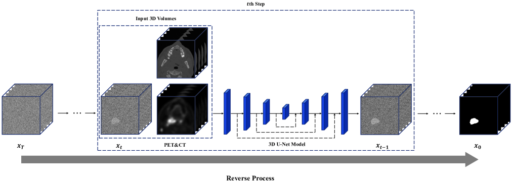
The graphic illustration of the proposed 3D diffusion model is shown in Figure 1. For our H&N segmentation task, both input and output data were represented in 3D form with size $D\times H\times W$, where $D$, $H$, and $W$ corresponded to dimensions in the depth (i.e., number of axial slices), height, and width directions, respectively. The targeted clean data $x_{0}$ was the 3D tumor mask. The reverse process involved the utilization of a neural network with parameters $\theta$ to restore the clean data $x_{0}$, typically employing a 2D U-Net. For our specific 3D segmentation task, we applied a 3D U-Net model to effectively capture all information across the three dimensions. The convolutional layers in this model employed 3D operations with kernel sizes of $(3,3,3)$. The kernel sizes for the downsample and upsample operations were set to $(1,2,2)$, trying to preserving the information along the axial direction. Additionally, we adopted the residual block as the fundamental unit in the model, as introduced in [27]. Regarding the hyper-parameters during the forward and reverse process, we designated a total of 1000 time steps ($T=1000$) and implemented a linear noise schedule for $\beta_{t}$. Table 1 shows a detailed list of parameter settings of our model.

Due to the substantial memory requirements of processing 3D multi-modality volumes, the batch size was set to 1. Moreover, to reduce the memory consumption and accelerate the training speed, we applied random cropping to the original volume, generating small volumes of size $32\times 96\times 96$ to train the model. Additionally, we employed data augmentation techniques, such as rotation and flipping, to enhance the diversity of the training data. The learning rate was set to $1\times 10^{-4}$, and a dropout rate of 0.1 was applied.

Reference Methods

We conducted a comparative analysis between our proposed 3D DDPM method and other state-of-the-art U-Net- and Transformer-based methods in the field of medical image segmentation. The reference models included the plain U-Net [3], nnU-Net [12], UNETR [17], and Swin UNETR [18]. To ensure a fair comparison, all models processed small 3D volumes with the size consistent with 3D DDPM. The trainable parameters for each model were also set to be the same as 3D DDPM. The validation set consisting of 18 cases was utilized to select the optimal checkpoints for all models in our study. The training of all the models was based on a single RTX8000 GPU (48 GB memory), the PyTorch platform and the Adam optimizer.

Data Analysis

We adopted four different metrics to quantitatively evaluate the segmentation results, including the Dice similarity coefficient (DSC), 95th percentile Hausdorff distance (HD), sensitivity, and specificity. DSC is a widely employed metric in segmentation tasks to measure the volumetric overlap between the segmentation output and the ground truth, defined as follows:

$$DSC(\hat{x}_{0},x_{0}^{GT})=\frac{2|\hat{x}_{0}\cap x_{0}^{GT}|}{|\hat{x}_{0}|+|x_{0}^{GT}|},$$ (10)

where $\hat{x}_{0}$ and $x_{0}^{GT}$ denote the output and ground-truth segmentation masks, respectively. HD measures the distance between the surfaces of the predicted tumor volumes and the surfaces of the ground-truth tumor volumes. To reduce the impact of outliers, the 95th percentile Hausdorff distance (HD95) is often preferred, calculated as follows:

$$HD95(\hat{x}_{0},x_{0}^{GT})=P_{95}( \max_{x\in\hat{x}_{0}}\min_{y\in x_{0}^{GT}}d(x,y),\max_{y\in x_{0}^{GT}}\min_{x\in\hat{x}_{0}}d(x,y)),$$ (11)

where $d(x,y)$ denotes the Euclidean distance between points $x$ and $y$, and $P_{95}$ is an operator extracting the 95th percentile. Furthermore, sensitivity and specificity are also widely utilized metrics. Specificity measures the true negative rate, indicating the model’s ability to correctly identify non-tumor regions, while sensitivity measures the model’s ability to accurately segment tumor regions. Balancing these metrics is vital for a reliable and accurate tumor segmentation model. Sensitivity and specificity are calculated as follows:

$$Sensitivity =\frac{TP}{TP+FN},$$ (12)

$$Specificity =\frac{TN}{FP+TN},$$ (13)

where $TP$, $TN$, $FP$, and $FN$ represent numbers of true positives, true negatives, false positives, and false negatives, respectively.

Results

Comparison with Other Reference Methods

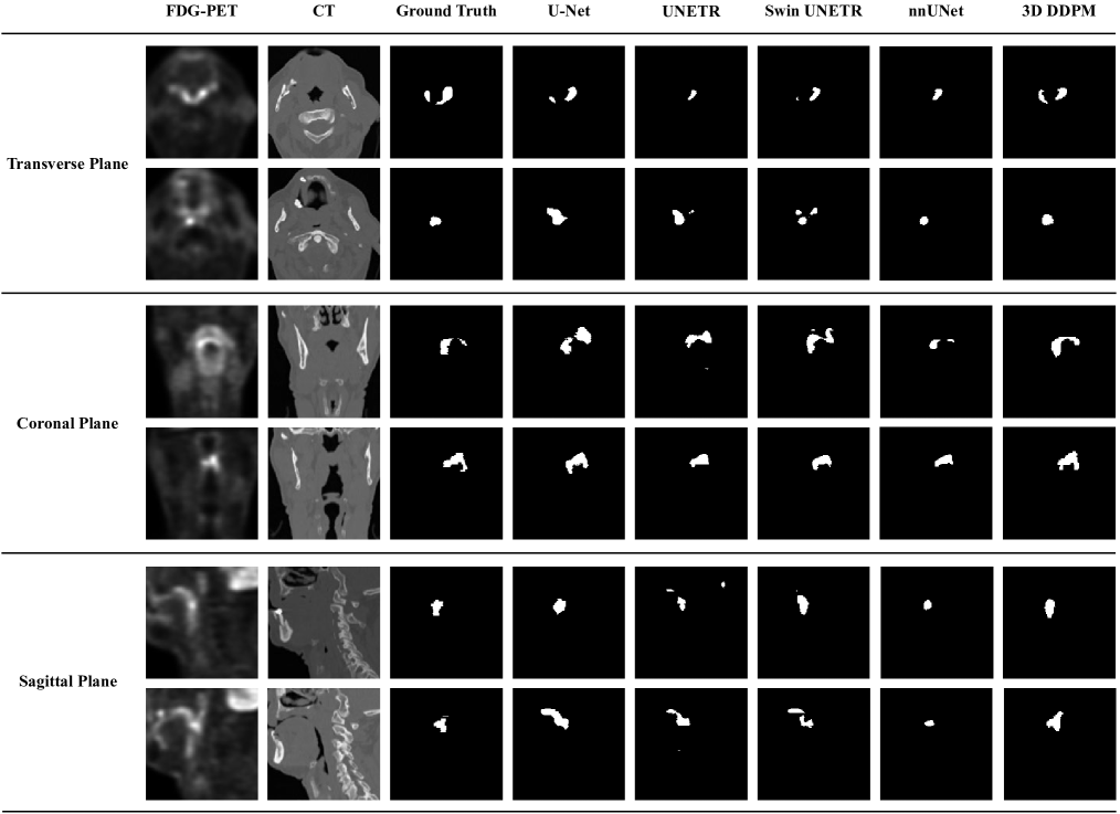
The qualitative and quantitative evaluation results of the proposed method and the four reference methods are shown in Figure 2 and Table 2, respectively. In Table 2, we calculated the average and standard deviation values across all testing cases for each method. The quantitative results showed that the proposed 3D DDPM achieved the highest DSC (0.733) and lowest HD95 (17.601) among all the reference methods; meanwhile, the nnU-Net attained the second-best DSC and HD95. We also noticed that incorporating the Transformer structure in UNETR could improve the performance as compared to the plain U-Net. The Swin UNETR, which employed the advanced Swin transformer structure, could further surpasses the performance of UNETR. Moreover, both the proposed 3D DDPM and nnU-Net achieved the highest specificity, revealing their excellent ability to correctly identify non-tumor regions. The proposed 3D DDPM model attained a higher sensitivity than nnU-Net, indicating its superior capability to accurately segment tumor regions.

This trend can also be observed in Figure 2. Referring to Table 2, it is evident that the plain U-Net model produced the highest sensitivity and the lowest specificity. Consequently, as shown in Figure 2, the plain U-Net tended to classify more pixels as tumor regions, resulting in more false positive errors. Conversely, both the UNETR and nnU-Net exhibited low sensitivity, as observed in the qualitative results, leading to the under-segmentation that missed numerous tumor regions. In comparison to these methods, the proposed 3D DDPM model attained the optimal balance between sensitivity and specificity, rendering it more effective for H&N tumor segmentation.

Comparison with 2D DDPM

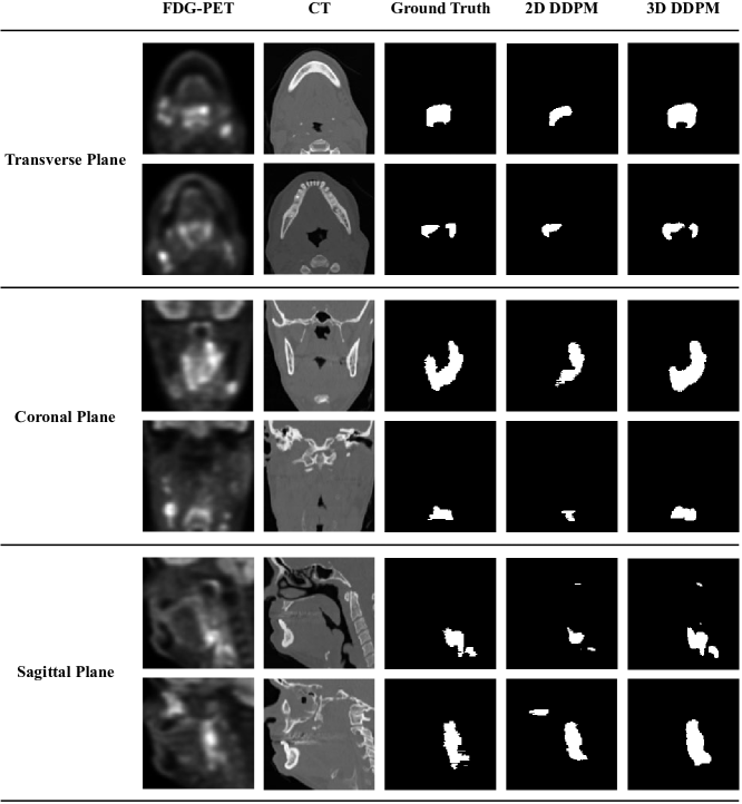
As previously mentioned, most existing diffusion models are in 2D format. In this work we proposed 3D DDPM to better extract the information existing between neighboring slices for 3D image segmentation. To demonstrate the effectiveness of 3D-based diffusion models, we conducted an experiment to compare the performance of 3D and 2D DDPM. The network structure utilized in 2D DDPM was set to be the same as that of 3D DDPM, except that 3D convolutional layers and down/up-sample layers were replaced by the corresponding 2D operations. The 2D DDPM was trained using 2D patches with the size of $96\times 96$, which were randomly cropped from 2D slices of the transverse view. We also ensured that the number of trainable parameters for the two models were the same. Quantitative and qualitative comparisons of 2D and 3D DDPM are presented in Table 3 and Figure 3, respectively. From the quantitative results in Table 3, it is obvious that 3D DDPM achieved the best performance across all four metrics. Qualitative results indicated that 2D DDPM tended to under-segment compared to 3D DDPM. These results demonstrate the importance of the information present among neighboring slices for image segmentation tasks, and also the benefits of further extending diffusion models from 2D to 3D.

Comparison with Single Modality-Based Segmentations

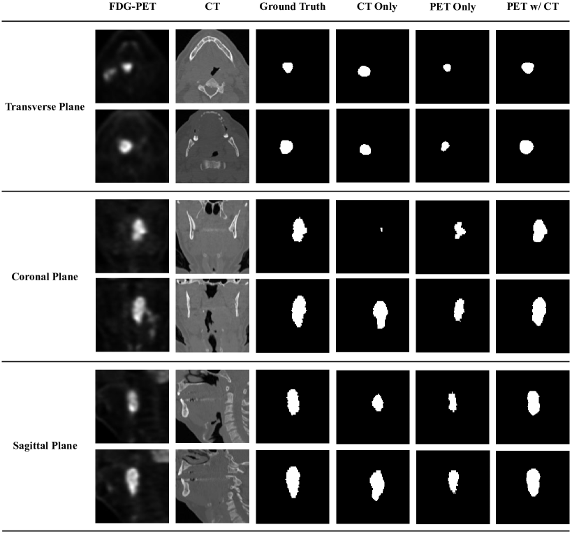
In the previous experiments, the input for all models consisted of dual-modality information obtained from both [¹⁸F]F-FDG PET and CT volumes, aiming to leverage the complementary information available from these distinct modalities. We further carried out an experiment to exam the effect of different modalities on the segmentation task by training the proposed 3D diffusion model using three different sets of input: 3D PET only, 3D CT only, and 3D PET combined with CT. All other aspects of the training process were kept be the same when varying the network input. Quantitative results of the 3D diffusion model with different network inputs are presented in Table 4. The comparative results clearly highlighted the superior performance achieved with dual-modality input. Furthermore, the model utilizing PET-only input achieved the second-best results, whereas the model relying on CT-only input performed significantly worse compared to the other two. This observation showed that [¹⁸F]F-FDG was more effective at delineating H&N tumors with high metabolic activities than CT images. These observations were consistent with the qualitative results presented in Figure 4. This experiment showed that integrating information from different modalities could effectively enhance the accuracy of H&N tumors delineation.

Comparison of Uncertainty Maps

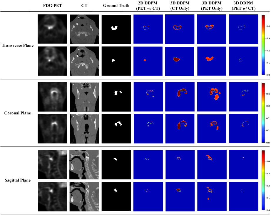
Stochasticity is one intrinsic property of diffusion models due to the randomly sampled Gaussian noise $x_{T}$ injected during the inference process. Consequently, for each inference process, the generated $x_{0}$ will have variations, even with the same conditional data. To explore the impact of this stochasticity, we repeated the inference process ten times and calculated the uncertainty maps accordingly. The models involved in this experiment included both 2D and 3D diffusion models with dual-modality inputs, along with 3D diffusion models with single-modality inputs. The qualitative results of uncertainty maps are illustrated in Figure 5. From the results, it is noteworthy that adding dual-modality inputs could significantly reduce the uncertainty of the diffusion model when comparing 2D/3D DDPM (PET and CT) to 3D DDPM (PET or CT only). Furthermore, compared with 2D DDPM (PET and CT), it is obvious that 3D DDPM (PET and CT) could further reduce the uncertainty of the generated H&N tumor segmentation masks. These observations validated that the proposed 3D diffusion model, utilizing dual-modality inputs, could effectively reduce the stochasticity, leading to the generation of more robust results.

Discussion

In this work, we extended the diffusion model to 3D format for the automatic H&N tumor segmentation based on 3D PET and CT volumes. Validations were conducted based on the publicly available HECKTOR 2021 dataset, which included over two hundred cases from various centers worldwide. Quantitative results showed that the proposed 3D diffusion model outperformed other reference models based on the U-Net and Transformer architectures (UNETR, Swin UNETR, and nnU-Net), achieving the best DSC and HD95 values. Furthermore, the proposed 3D diffusion model achieved the best balance between sensitivity and specificity. Experiments were also conducted to compare the performance of the diffusion model in 2D and 3D formats, highlighting the effectiveness of extracting 3D features from 3D PET and CT volumes. Performance of the 3D diffusion model with dual-modality and single-modality inputs was also evaluated, which demonstrated the effectiveness of leveraging complementary information from different imaging modalities. Additionally, the comparison of uncertainty maps provided further evidence of the 3D diffusion model’s capability in effectively reducing the stochasticity.

While the diffusion model has demonstrated outstanding performance, its primary drawbacks are the high computational demand and slow processing speed. As previously explained, during the reverse process, the clean data $x_{0}$ was gradually reconstructed from the initial random Gaussian distribution $x_{T}$ step by step. Typically, the time step $T$ was set to 1000 [20] and thus the reverse process needed to iterate 1000 times during each inference. To address this issue, researchers have proposed various techniques to reduce the number of time steps, e.g. , DDIM [28], DPMSolver [29], and Analytic-DPM [30]. In the future, we plan to explore these techniques to reduce the inference time of the diffusion model, making it more efficient and practical for the image segmentation task.

In this work, the dataset utilized for training and testing all models was the HECKTOR 2021 dataset, which included 224 cases from 5 centers worldwide. In our future work, we plan to train and evaluate the proposed framework based on datasets from additional cohorts to encompass a broader spectrum of patients, which can contribute to more comprehensive and robust model training and validation. The diffusion model is a general framework where various neural network structures can be employed to generate the output from the Gaussian noise and the conditional input. In our work, due to limitations in GPU memory and computational speed, we utilized a 3D U-Net model without any attention mechanism within the diffusion framework. Employing a more powerful neural network architect, such as the Transformer structure and the newly proposed structured state space models [31, 32], can potentially enhance the performance of the diffusion model, which is also one of our future research directions.

Conclusion

In this work, we developed a 3D diffusion model to perform automated H&N tumor segmentation from [¹⁸F]F-FDG PET and CT images. The diffusion model employed a 3D UNet model and utilized the concatenation of 3D PET, CT, and Gaussian noise volumes as the network inputs. Effectiveness of the proposed diffusion model was validated through the comparison with other state-of-the-art methods based on the U-Net and Transformers. Both qualitative and quantitative results demonstrated that the proposed 3D diffusion model could generate more accurate H&N tumor segmentation masks compared to the other reference methods.

Statements and Declarations

Funding This work was supported by the National Institutes of Health under grants R21AG067422, R03EB030280, R01AG078250, and P41EB022544.

Competing Interests The authors have no relevant financial or non-financial interests to disclose..

Ethics approval All procedures performed in studies involving human participants were in accordance with the ethical standards of the institutional and/or national research committee and with the 1964 Helsinki declaration and its later amendments or comparable ethical standards.

Informed consent Informed consent was waived due to the retrospective merits of the datasets.

Figure 1: Graphic illustration for our proposed 3D diffusion model. In the reverse process, the model took 3D FDG-PET, CT, and Gaussian distribution volumes as input and restored the 3D tumor masks step by step.

Figure 2: Three views of the H&N segmentation results generated by different methods based on one test dataset.

Figure 3: Three views of H&N segmentation results from the diffusion models in 2D and 3D forms based on one test dataset.

Figure 4: Three views of H&N segmentation results from the 3D diffusion models with different input modalities based on one test dataset.

Figure 5: Three views of the uncertainty maps of H&N tumor segmentation results. These uncertainty maps were generated based on different DDPM-based methods for one test dataset.

Table 1: List of detailed hyper-parameters of the proposed 3D diffusion model. For input and output dimensions, $N$ denotes the batch size. The base channels represent the dimensions of the initial layer, whereas the channel multipliers serve as factors that are multiplied by the base channels for subsequent layers.

Hyper-parameter	Value
Input Dimension	$N\times 3\times 32\times 96\times 96$
Output Dimension	$N\times 1\times 32\times 96\times 96$
Convolutional Kernel Size	$(3,3,3)$
Down/up-sample Kernel Size	$(1,2,2)$
Diffusion Steps	1000
Noise Schedule	Linear
Base Channels	128
Channel Multiplier	$(1,1,2,3,4)$
Residual Blocks	2
Model Size	214M

Table 2: Quantitative evaluation results (DSC, HD95, sensitivity, specificity, and corresponding standard deviation values) of different methods. Note that $\uparrow$ indicates that larger values provide better results, while $\downarrow$ indicates the opposite. Bold indicates the best performance, while underline indicates the second best.

	DSC ($\uparrow$)	HD95 ($\downarrow$)	Sensitivity ($\uparrow$)	Specificity ($\uparrow$)
U-Net	0.641 ($\pm$0.225)	60.606 ($\pm$35.149)	0.743 ($\pm$0.217)	0.996 ($\pm$0.003)
UNETR	0.648 ($\pm$0.215)	43.437 ($\pm$31.792)	0.676 ($\pm$0.225)	0.998 ($\pm$0.002)
Swin UNETR	0.695 ($\pm$0.210)	26.326 ($\pm$28.196)	0.728 ($\pm$0.226)	0.998 ($\pm$0.002)
nnU-Net	0.719 ($\pm$0.218)	17.971 ($\pm$31.670)	0.683 ($\pm$0.238)	0.999 ($\pm$0.001)
3D DDPM	0.733 ($\pm$0.198)	17.601 ($\pm$25.447)	0.729 ($\pm$0.240)	0.999 ($\pm$0.002)

Table 3: Quantitative evaluation results (DSC, HD95, sensitivity, specificity, and corresponding standard deviation values) of the 3D and 2D diffusion models. Note that $\uparrow$ indicates that larger values provide better results, while $\downarrow$ indicates the opposite. Bold indicates the best performance.

	DSC ($\uparrow$)	HD95 ($\downarrow$)	Sensitivity ($\uparrow$)	Specificity ($\uparrow$)
2D DDPM	0.664 ($\pm$0.221)	18.903 ($\pm$22.607)	0.645 ($\pm$0.256)	0.999 ($\pm$0.001)
3D DDPM	0.733 ($\pm$0.198)	17.601 ($\pm$25.447)	0.729 ($\pm$0.240)	0.999 ($\pm$0.002)

Table 4: Quantitative evaluation results (DSC, HD95, Sensitivity, Specificity, and corresponding standard deviation values) of the 3D diffusion models with different modalities as the network. Note that $\uparrow$ indicates that larger values provide better results, while $\downarrow$ indicates the opposite. Bold indicates the best performance, while underline indicates the second best.

	DSC ($\uparrow$)	HD95 ($\downarrow$)	Sensitivity ($\uparrow$)	Specificity ($\uparrow$)
CT Only	0.297 ($\pm$0.252)	44.237 ($\pm$38.810)	0.272 ($\pm$0.242)	0.998 ($\pm$0.002)
FDG-PET Only	0.575 ($\pm$0.230)	30.246 ($\pm$28.306)	0.651 ($\pm$0.221)	0.997 ($\pm$0.003)
FDG-PET w/ CT	0.733 ($\pm$0.198)	17.601 ($\pm$25.447)	0.729 ($\pm$0.240)	0.999 ($\pm$0.002)

References

- [1] A. Argiris, M. V. Karamouzis, D. Raben, and R. L. Ferris, “Head and neck cancer,” The Lancet, vol. 371, no. 9625, pp. 1695–1709, 2008.
- [2] T. Gupta, Z. Master, S. Kannan, J. P. Agarwal, S. Ghsoh-Laskar, V. Rangarajan, V. Murthy, and A. Budrukkar, “Diagnostic performance of post-treatment fdg pet or fdg pet/ct imaging in head and neck cancer: a systematic review and meta-analysis,” European journal of nuclear medicine and molecular imaging, vol. 38, pp. 2083–2095, 2011.
- [3] O. Ronneberger, P. Fischer, and T. Brox, “U-net: Convolutional networks for biomedical image segmentation,” in Medical Image Computing and Computer-Assisted Intervention–MICCAI 2015: 18th International Conference, Munich, Germany, October 5-9, 2015, Proceedings, Part III 18, pp. 234–241, Springer, 2015.
- [4] R. Azad, E. K. Aghdam, A. Rauland, Y. Jia, A. H. Avval, A. Bozorgpour, S. Karimijafarbigloo, J. P. Cohen, E. Adeli, and D. Merhof, “Medical image segmentation review: The success of u-net,” arXiv preprint arXiv:2211.14830, 2022.
- [5] Z. Guo, N. Guo, K. Gong, Q. Li, et al., “Gross tumor volume segmentation for head and neck cancer radiotherapy using deep dense multi-modality network,” Physics in Medicine & Biology, vol. 64, no. 20, p. 205015, 2019.
- [6] Z. Zhou, M. M. R. Siddiquee, N. Tajbakhsh, and J. Liang, “Unet++: Redesigning skip connections to exploit multiscale features in image segmentation,” IEEE transactions on medical imaging, vol. 39, no. 6, pp. 1856–1867, 2019.
- [7] H. Huang, L. Lin, R. Tong, H. Hu, Q. Zhang, Y. Iwamoto, X. Han, Y.-W. Chen, and J. Wu, “Unet 3+: A full-scale connected unet for medical image segmentation,” in ICASSP 2020-2020 IEEE international conference on acoustics, speech and signal processing (ICASSP), pp. 1055–1059, IEEE, 2020.
- [8] T. Xiang, C. Zhang, D. Liu, Y. Song, H. Huang, and W. Cai, “Bio-net: learning recurrent bi-directional connections for encoder-decoder architecture,” in Medical Image Computing and Computer Assisted Intervention–MICCAI 2020: 23rd International Conference, Lima, Peru, October 4–8, 2020, Proceedings, Part I 23, pp. 74–84, Springer, 2020.
- [9] O. Oktay, J. Schlemper, L. L. Folgoc, M. Lee, M. Heinrich, K. Misawa, K. Mori, S. McDonagh, N. Y. Hammerla, B. Kainz, et al., “Attention u-net: Learning where to look for the pancreas,” arXiv preprint arXiv:1804.03999, 2018.
- [10] C. Li, Y. Tan, W. Chen, X. Luo, Y. Gao, X. Jia, and Z. Wang, “Attention unet++: A nested attention-aware u-net for liver ct image segmentation,” in 2020 IEEE international conference on image processing (ICIP), pp. 345–349, IEEE, 2020.
- [11] Ö. Çiçek, A. Abdulkadir, S. S. Lienkamp, T. Brox, and O. Ronneberger, “3d u-net: learning dense volumetric segmentation from sparse annotation,” in Medical Image Computing and Computer-Assisted Intervention–MICCAI 2016: 19th International Conference, Athens, Greece, October 17-21, 2016, Proceedings, Part II 19, pp. 424–432, Springer, 2016.
- [12] F. Isensee, P. F. Jaeger, S. A. Kohl, J. Petersen, and K. H. Maier-Hein, “nnu-net: a self-configuring method for deep learning-based biomedical image segmentation,” Nature methods, vol. 18, no. 2, pp. 203–211, 2021.
- [13] A. Vaswani, N. Shazeer, N. Parmar, J. Uszkoreit, L. Jones, A. N. Gomez, Ł. Kaiser, and I. Polosukhin, “Attention is all you need,” Advances in neural information processing systems, vol. 30, 2017.
- [14] S.-I. Jang, T. Pan, Y. Li, P. Heidari, J. Chen, Q. Li, and K. Gong, “Spach transformer: spatial and channel-wise transformer based on local and global self-attentions for pet image denoising,” IEEE Transactions on Medical Imaging, 2023.
- [15] J. Chen, Y. Lu, Q. Yu, X. Luo, E. Adeli, Y. Wang, L. Lu, A. L. Yuille, and Y. Zhou, “Transunet: Transformers make strong encoders for medical image segmentation,” arXiv preprint arXiv:2102.04306, 2021.
- [16] A. Dosovitskiy, L. Beyer, A. Kolesnikov, D. Weissenborn, X. Zhai, T. Unterthiner, M. Dehghani, M. Minderer, G. Heigold, S. Gelly, et al., “An image is worth 16x16 words: Transformers for image recognition at scale,” arXiv preprint arXiv:2010.11929, 2020.
- [17] A. Hatamizadeh, Y. Tang, V. Nath, D. Yang, A. Myronenko, B. Landman, H. R. Roth, and D. Xu, “Unetr: Transformers for 3d medical image segmentation,” in Proceedings of the IEEE/CVF winter conference on applications of computer vision, pp. 574–584, 2022.
- [18] A. Hatamizadeh, V. Nath, Y. Tang, D. Yang, H. R. Roth, and D. Xu, “Swin unetr: Swin transformers for semantic segmentation of brain tumors in mri images,” in International MICCAI Brainlesion Workshop, pp. 272–284, Springer, 2021.
- [19] Z. Liu, Y. Lin, Y. Cao, H. Hu, Y. Wei, Z. Zhang, S. Lin, and B. Guo, “Swin transformer: Hierarchical vision transformer using shifted windows,” in Proceedings of the IEEE/CVF international conference on computer vision, pp. 10012–10022, 2021.
- [20] J. Ho, A. Jain, and P. Abbeel, “Denoising diffusion probabilistic models,” Advances in Neural Information Processing Systems, vol. 33, pp. 6840–6851, 2020.
- [21] P. Dhariwal and A. Nichol, “Diffusion models beat gans on image synthesis,” Advances in neural information processing systems, vol. 34, pp. 8780–8794, 2021.
- [22] C. Saharia, J. Ho, W. Chan, T. Salimans, D. J. Fleet, and M. Norouzi, “Image super-resolution via iterative refinement,” IEEE Transactions on Pattern Analysis and Machine Intelligence, vol. 45, no. 4, pp. 4713–4726, 2022.
- [23] K. Gong, K. Johnson, G. El Fakhri, Q. Li, and T. Pan, “Pet image denoising based on denoising diffusion probabilistic model,” European Journal of Nuclear Medicine and Molecular Imaging, pp. 1–11, 2023.
- [24] R. Rombach, A. Blattmann, D. Lorenz, P. Esser, and B. Ommer, “High-resolution image synthesis with latent diffusion models,” in Proceedings of the IEEE/CVF conference on computer vision and pattern recognition, pp. 10684–10695, 2022.
- [25] J. Wu, H. Fang, Y. Zhang, Y. Yang, and Y. Xu, “Medsegdiff: Medical image segmentation with diffusion probabilistic model,” arXiv preprint arXiv:2211.00611, 2022.
- [26] V. Andrearczyk, V. Oreiller, S. Boughdad, C. C. L. Rest, H. Elhalawani, M. Jreige, J. O. Prior, M. Vallières, D. Visvikis, M. Hatt, et al., “Overview of the hecktor challenge at miccai 2021: automatic head and neck tumor segmentation and outcome prediction in pet/ct images,” in 3D head and neck tumor segmentation in PET/CT challenge, pp. 1–37, Springer, 2021.
- [27] A. Brock, J. Donahue, and K. Simonyan, “Large scale gan training for high fidelity natural image synthesis,” arXiv preprint arXiv:1809.11096, 2018.
- [28] J. Song, C. Meng, and S. Ermon, “Denoising diffusion implicit models,” arXiv preprint arXiv:2010.02502, 2020.
- [29] C. Lu, Y. Zhou, F. Bao, J. Chen, C. Li, and J. Zhu, “Dpm-solver: A fast ode solver for diffusion probabilistic model sampling in around 10 steps,” Advances in Neural Information Processing Systems, vol. 35, pp. 5775–5787, 2022.
- [30] F. Bao, C. Li, J. Zhu, and B. Zhang, “Analytic-dpm: an analytic estimate of the optimal reverse variance in diffusion probabilistic models,” arXiv preprint arXiv:2201.06503, 2022.
- [31] A. Gu, K. Goel, and C. Ré, “Efficiently modeling long sequences with structured state spaces,” arXiv preprint arXiv:2111.00396, 2021.
- [32] A. Gu and T. Dao, “Mamba: Linear-time sequence modeling with selective state spaces,” arXiv preprint arXiv:2312.00752, 2023.