A simple method to measure $\boldsymbol{\nu}_{\rm\bf max}$ for asteroseismology: application to 16,000 oscillating Kepler red giants

Abstract

The importance of $\nu_{\rm max}$ (the frequency of maximum oscillation power) for asteroseismology has been demonstrated widely in the previous decade, especially for red giants. With the large amount of photometric data from CoRoT, Kepler and TESS, several automated algorithms to retrieve $\nu_{\rm max}$ values have been introduced. Most of these algorithms correct the granulation background in the power spectrum by fitting a model and subtracting it before measuring $\nu_{\rm max}$. We have developed a method that does not require fitting to the granulation background. Instead, we simply divide the power spectrum by a function of the form $\rm\nu^{-2}$, to remove the slope due to granulation background, and then smooth to measure $\nu_{\rm max}$. This method is fast, simple and avoids degeneracies associated with fitting. The method is able to measure oscillations in 99.9 % of previously-studied Kepler red giants, with a systematic offset in $\nu_{\rm max}$ values that depends upon the evolutionary state. On comparing the seismic radii from this work with Gaia, we see similar trends to those observed in previous studies. Additionally, our values of width of the power envelope can clearly identify the dipole mode suppressed stars as a distinct population, hence as a way to detect them. We also applied our method to stars with low $\nu_{\rm max}$ (0.39–18.35 $\mu$Hz) and found it works well to correctly identify the oscillations.

1 Introduction

The space-based photometric missions like CoRoT (Convection, Rotation and planetary Transits), Kepler and TESS (Transiting Exoplanet Survey Satellite) have measured low-amplitude oscillations in very large samples of red giants (see reviews by Chaplin & Miglio 2013; Jackiewicz 2021). These results were mostly obtained by algorithms that derive two main seismic parameters: the frequency of maximum oscillation power ($\nu_{\rm max}$) and the large frequency separation ($\Delta\nu$), which in turn yield the stellar mass and radius. To a good approximation, $\nu_{\rm max}$ is proportional to $g/\sqrt{T_{\rm eff}}$ (Brown et al., 1991; Kjeldsen & Bedding, 1995; Bedding & Kjeldsen, 2003; Belkacem et al., 2011; Hekker, 2020). With the addition of the stellar luminosity from Gaia, $\nu_{\rm max}$ can be used to estimate mass without measuring $\rm\Delta\nu$ (Miglio et al., 2012; Hon et al., 2021). Here we focus on measuring $\nu_{\rm max}$, using a new and simple approach.

Most of the existing algorithms model and remove the granulation signal by fitting the components of one or more Harvey models (Harvey, 1985; Huber et al., 2009; Mosser & Appourchaux, 2009; Mathur et al., 2010; Kallinger et al., 2010; Hekker et al., 2010; Gehan et al., 2023), with a few exceptions such as the machine learning analysis by Hon et al. (2018, 2019, 2021) and the method using Coefficient of Variation by Bell et al. (2019). The process of fitting the granulation background is fairly complicated and may involve a degeneracy between parameter sets (Mathur et al., 2011; Kallinger et al., 2014). Furthermore, one has to rely on model comparison and sampling techniques to solve this degeneracy, which may not be suitable while dealing with large number of stars. This motivated us to explore a method without background fitting, given we only need to measure seismic parameters. We have developed a pipeline (nuSYD) in which we divide the power spectrum by a function of the form $\rm\nu^{-2}$, to remove the slope due to the granulation background, and then smooth to measure $\nu_{\rm max}$. Our method is simple and quick, and the results for Kepler red giants agree well with the previous measurements.

2 Data and Methods

The method used by our nuSYD pipeline can be summarised as follows:

1. Calculate the power density spectrum of the light curve (Sec. 2.1).

2. Estimate an initial value for $\nu_{\rm max}$, based on the mean power in the power spectrum (Sec. 2.2).

3. Measure and subtract the white noise (Sec.  2.3).

4. Remove the slope of the granulation background by dividing the power density spectrum by $\Big{(}\frac{\nu}{\mbox{$\nu_{\rm max}$}}\Big{)}^{-2}$ ( Sec. 2.4).

5. Heavily smooth the power density spectrum, using a Gaussian whose width is a simple function of $\nu_{\rm max}$ (Sec. 2.5).

We carried out steps (iii)–(v) for a total of three times, using the new value of $\nu_{\rm max}$ in each iteration. We measured $\nu_{\rm max}$, the peak power ($P_{\rm peak}$) and the width ($W$) from the final smoothed envelope. We discuss our method of estimating uncertainties in Sec. 2.6.

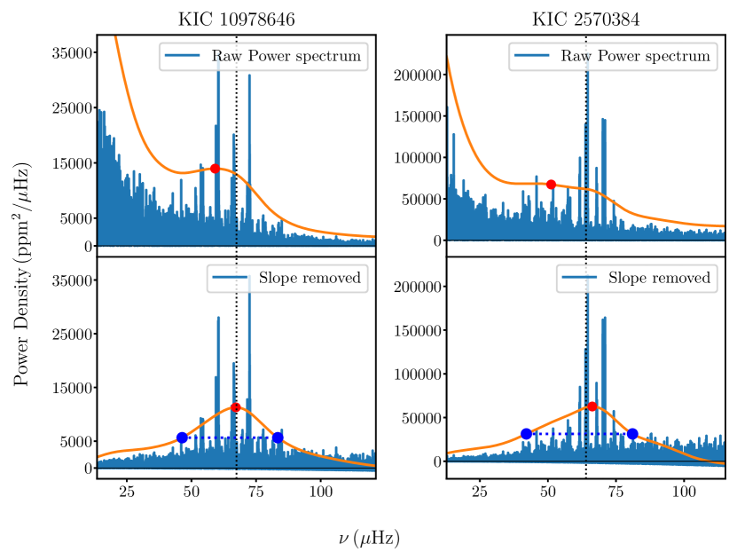
Figure 1: Illustration of our method for stars KIC 10978646 and KIC 257084. The orange curves show smoothed power spectra (scaled in the vertical direction for better visibility) and the red dots show the $\nu_{\rm max}$ values. Upper panels are without removing the background slope (step iv omitted), and lower panels show the final result after background division. The blue dashed lines show $W$ connecting the two half-power points, and the vertical black dashed line shows $\nu_{\rm max}$ reported by Yu et al. (2018).

Figure 1 illustrates the results using two typical red giants. The upper panels show the results when step (iv) is not included in the process. This is successful in measuring $\nu_{\rm max}$ for around 80% stars in Yu et al. (2018), including KIC 10978646 (upper left panel). There is obviously a systematic bias, but this could be calibrated. However, the method did not work for stars like KIC 2570384, which has weak oscillation modes compared to the background power on lower frequencies (upper right panel). This motivated us to adopt the additional step of removing the slope of the granulation background, to give the final values for $\nu_{\rm max}$, $P_{\rm peak}$ and $W$ (lower panels).

2.1 Pre-processing light curves and calculating power spectra

For all 16094 targets in Yu et al. (2018) we downloaded all four years of Kepler long-cadence PDCSAP (Pre-search Data Conditioning Simple Aperture Photometry) light curves (Stumpe et al., 2012; Smith et al., 2012), using the Mikulski Archive for Space Telescope (MAST), Data Release 25. In order to remove the low-frequency variations due to stellar activity and instrumental noise that were sometimes not corrected by PDCSAP, we high-pass filtered all the light curves by convolution with a Gaussian kernel of width 10 d, and dividing out these slow variations. We then calculated power spectra up to the Nyquist frequency ($\rm\nu_{Nyq}$ = 283.2 $\mu$Hz). The power (in ppm²) was converted to power density (in ppm²/$\mu$Hz), by multiplying by the effective time span of the observations, which we calculated as 29.4 min times the number of data points. For the 168 stars in Colman et al. (2017) that have anomalous peaks (probably due to a close binary that is contaminating the light curve), we replaced the anomalous peaks with the median of the power spectra in a 1 $\mu$Hz region around each peak.

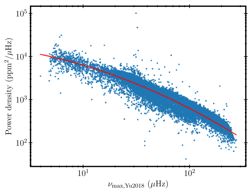
Figure 2: Mean level in the power density from the power spectra, as a function of $\nu_{\rm max}$ from Yu et al. 2018. The red line shows the fit in Eq. 1.

2.2 Calculating the initial $\nu_{\rm max}$

Since the next two steps in the nuSYD pipeline depend upon $\nu_{\rm max}$, we required an initial value for each star. We used a fairly crude estimate that relies on the fact that $\nu_{\rm max}$ scales inversely with the power in both the oscillation signal and the granulation background (Mathur et al., 2011; Hekker et al., 2012; Kallinger et al., 2016; Yu et al., 2018; Bugnet et al., 2018). We measured this stellar power ($P_{\rm stellar}$) as the mean power density in the frequency range from 5 $\mu$Hz to $\rm\nu_{Nyq}$, minus the mean noise in the region above 0.97 $\rm\nu_{Nyq}$ (274.7– 283.2 $\mu$Hz). The results are shown in Fig. 2. This is the same metric as used by Bugnet et al. (2018) for estimating surface gravities. We fitted a quadratic function (red curve) and hence obtained an approximate relation for $\nu_{\rm max}$ as a function of mean level ($P_{\rm stellar}$) in the power density spectrum:

$$\log_{10}\Bigg{(}\frac{\nu_{\rm max}}{\rm\mu Hz}\Bigg{)}=3.08-0.0824\,\log_{10}\Bigg{(}\frac{P_{\rm stellar}}{{\rm ppm^{2}/\mu Hz}}\Bigg{)}-\\ 0.115\,\Bigg{(}\log_{10}\Bigg{(}\frac{P_{\rm stellar}}{{\rm ppm^{2}/\mu Hz}}\Bigg{)}\Bigg{)}^{2}$$ (1)

For each star, we used the mean level in the power density spectrum to obtain an initial $\nu_{\rm max}$ using this relation. If the predicted $\nu_{\rm max}$ was greater than $\rm\nu_{Nyq}$, we set the initial $\nu_{\rm max}$ at $\rm\nu_{Nyq}$. We note that for most of the stars (99.85%), we found that final results were not sensitive to the initial estimate.

2.3 Estimating the high-frequency noise

Generally, the white noise in a power spectrum is calculated at high frequencies, above the region containing the oscillations and granulation background. Our sample contains some stars whose $\nu_{\rm max}$ is close to the Nyquist frequency (see Yu et al. 2016), and we estimated the white noise differently for those stars. For initial $\nu_{\rm max}$ less than 0.9 $\rm\nu_{Nyq}$ (254.9 $\mu$Hz, which is 99.91% of the sample), we estimated the white noise as the mean power density in the region 0.97 $\rm\nu_{Nyq}$ to $\rm\nu_{Nyq}$ (274.7–283.2 $\mu$Hz), but for $\nu_{\rm max}$ greater than 0.9 $\rm\nu_{Nyq}$, we estimated in the region from 0.6 $\nu_{\rm max}$ to 0.7 $\nu_{\rm max}$.

Figure 3 shows the relation between high-frequency noise and Kepler magnitude for all stars in our sample. As expected, there is a correlation with the Kepler magnitude (see also Gilliland et al. 2010; Jenkins et al. 2010; Pande et al. 2018). It should be noted that for bright stars, our determination of high-frequency noise actually includes granulation noise, which causes the upturn at low K_p values.

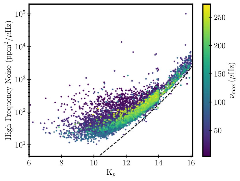
Figure 3: High frequency noise (in ppm²/$\mu$Hz) as a function of Kepler magnitude, color coded with $\nu_{\rm max}$ values. The black dashed line shows the lower envelope of white noise measured by Jenkins et al. 2010.

2.4 Removing the background slope

A fit to the background generally involves fitting one or more Harvey models, each with several free parameters (Harvey, 1985; Mathur et al., 2011; Mosser et al., 2012; Kallinger et al., 2014). Instead, we simply removed the slope of the background noise by dividing the power density spectra by $\Big{(}\frac{\nu}{\mbox{$\nu_{\rm max}$}}\Big{)}^{-2}$. This function has a value of 1 at $\nu_{\rm max}$.

We chose an exponent of $-2$ to be consistent with the Harvey model and we note that Mosser et al. (2012) measured the exponent to be $-2.1\pm 0.3$, which is consistent with this value. We checked the effect on all stars of changing the exponent from $-2$ to $-2.1$ and found that the offset in $\nu_{\rm max}$ is only a few tenths of a percent.

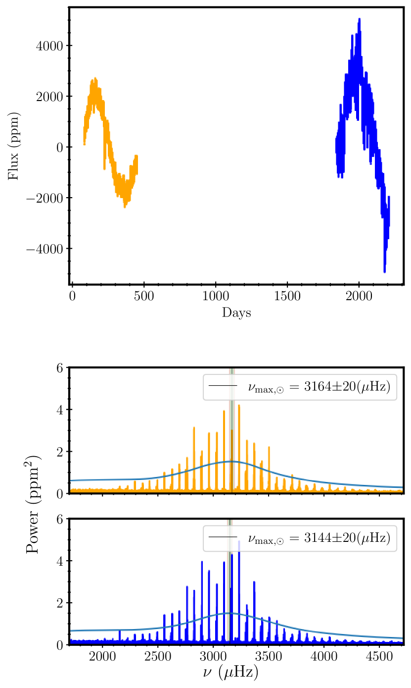
Figure 4: $\rm\nu_{max,\odot}$ from VIRGO composite time series using our method. Top panel shows the time series from 1996 (orange) and 2001 (blue). Middle panel shows the corresponding power spectra (orange) and corresponding smoothed one (light blue), for the year 1996. The bottom panel shows the power spectra (blue) and smoothed power spectra (light blue) for the year 2001. The vertical line shows the $\nu_{\rm max}$ measured and the green region represents the corresponding error bar. The smoothed spectra have been scaled in the vertical direction for better visibility.

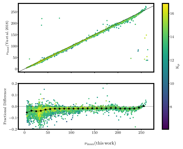
Figure 5: Comparison of $\nu_{\rm max}$ values with Yu et al. (2018). The diagonal black line corresponds to the one-to-one line. The lower panel shows the fractional difference: $\left(\mbox{$\nu_{\rm max,Yu+2018}$}{}-\mbox{$\nu_{\rm max}$}{}\right)/\mbox{$\nu_{\rm max}$}$ and the points are colour-coded by Kepler magnitude. The black stars represent the medians in bins with a width of 10 $\mu$Hz.

2.5 Smoothing and determining seismic parameters

In order to locate and measure the power excess, we smoothed the power spectrum by convolution with a Gaussian kernel. From previous studies we know that the optimum width of the smoothing function is proportional to the large frequency separation ($\rm\Delta\nu$). For main-sequence stars, Kjeldsen et al. (2005) suggested a FWHM of 4 $\rm\Delta\nu$, in order to smooth out the structure from individual modes. In the SYD pipeline developed by Huber et al. (2009) and used by Yu et al. (2018), and also in its python implementation (Chontos et al., 2021), the width of the smoothing function is $\mbox{$\Delta\nu$}*\max\left(1,4\,(\mbox{$\nu_{\rm max}$}/\nu_{\rm max,\odot})^{0.2}\right)$. For this work, we tried a simpler formula using different values for FWHM, and 2 $\rm\Delta\nu$ gave good results across the entire sample of red giants. As in SYD, we estimated $\rm\Delta\nu$ from $\nu_{\rm max}$ using the approximate relation $\rm\Delta\nu=0.26\,\left(\frac{\mbox{$\nu_{\rm max}$}{}}{\rm\mu Hz}\right)^{0.772}$ (Stello et al., 2009; Huber et al., 2011).

We defined a search window around the initial $\nu_{\rm max}$, which ranged from 0.5 $\nu_{\rm max}$ to 2 $\nu_{\rm max}$. We then measured $\nu_{\rm max}$ as the frequency corresponding to the maximum in the smoothed power spectra within this window, and the power at $\nu_{\rm max}$ ($P_{\rm peak}$) as the peak power of the envelope (which includes both oscillations and granulation). We also determined the width ($W$ in $\mu$Hz) as the distance between the half-power points of the envelope.

We repeated this procedure of white-noise subtraction, background division and smoothing for a total of three times. The lower panels of Fig. 1 show two examples. Additionally in the final iteration, we corrected for the non-zero integration times (sometimes called apodization) by dividing the white-noise subtracted power spectra by $\operatorname{sinc}^{2}\left(\frac{\pi}{2}\frac{\nu}{\rm\nu_{Nyq}}\right)$ (Huber et al., 2009; Chaplin et al., 2011; Kallinger et al., 2014).

2.6 Calculating uncertainties

When a long data set is available, the measurement uncertainties can be determined directly by subdividing the data into shorter segments and calculating the scatter. To estimate uncertainties in our results, we divided the Kepler light curve of each star into quarters and performed one iteration of our algorithm, using our measured $\nu_{\rm max}$ as the initial value. This yielded a list of $\nu_{\rm max}$, $P_{\rm peak}$ and $W$ for each quarter. The standard deviation of this list divided by the square root of the number of quarters gave the uncertainties associated with each parameter, for each star. These should be realistic estimates of the random uncertainties, since they include contributions from the variations due to stochastic nature of oscillations, as well as the noise from photon statistics. They do not include possible systematic uncertainties such as variations with stellar activity and any effects from the choice of the method. We also calculated uncertainties using Monte Carlo simulations, as described by Huber et al. (2011), and found these to be slightly lower than the values described above, presumably because the Monte Carlo method does not account for variations over the four-year mission due to stochastic nature of oscillations.

3 Discussion

3.1 Application to solar data

It is conventional for each pipeline to be calibrated with reference to the Sun (Pinsonneault et al., 2018). In order to calibrate our method on the Sun, we followed Huber et al. (2011) in using photometric data from VIRGO (Variability of Solar Irradiance and Gravity Oscillations; Fröhlich et al. 1995 ), installed onboard of SOHO (Solar and Heliospheric Observatory). The VIRGO instrument observed the Sun through three channels at 862 nm (Red), 500 nm (Green) and 402 nm (Blue). It made observations from 1996 to 2017 with a cadence of 60 seconds. A composite time series that has a bandwidth closest to Kepler’s can be obtained by adding observations from the Green and Red VIRGO channels (Basri et al., 2010; Salabert et al., 2017). We applied our method to the three individual channel light curves and to the composite light curve.

The uncertainties on $\nu_{\rm max,\odot}$ for each light curve were obtained by applying our method to 25 d long, non-overlapping sections (see Sec. 2.6). Figure 4 shows the result for the 1996 and 2001 VIRGO composite time series. The $\nu_{\rm max,\odot}$ values are 3164 $\pm$ 20  $\mu$Hz and 3144 $\pm$ 20  $\mu$Hz, which agree within the uncertainty (see also Howe et al., 2020; Kim & Chang, 2022). These values are within the range measured by the various other pipelines (Table 1 of Pinsonneault et al. 2018). We adopt an average value of $\mbox{$\nu_{\rm max,\odot}$}=3154\,\pm\,30$, which is 2% higher than the value measured using the SYD pipeline ($\rm\nu_{max,\odot}=3090\pm 30\mbox{$\mu$}Hz$; Huber et al. 2011). This difference is caused by the different ways the two methods treat the granulation background, as discussed in the next section.

3.2 Comparison with Yu et al. (2018)

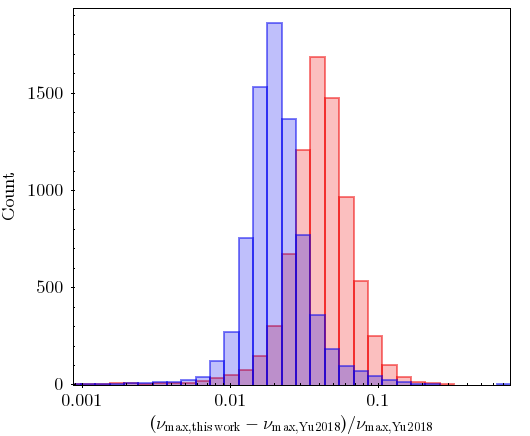
Figure 6: Comparison of offsets in $\nu_{\rm max}$ values, among RGB and RC stars. The blue bins correspond to RGB stars and red bins correspond to red clump stars.

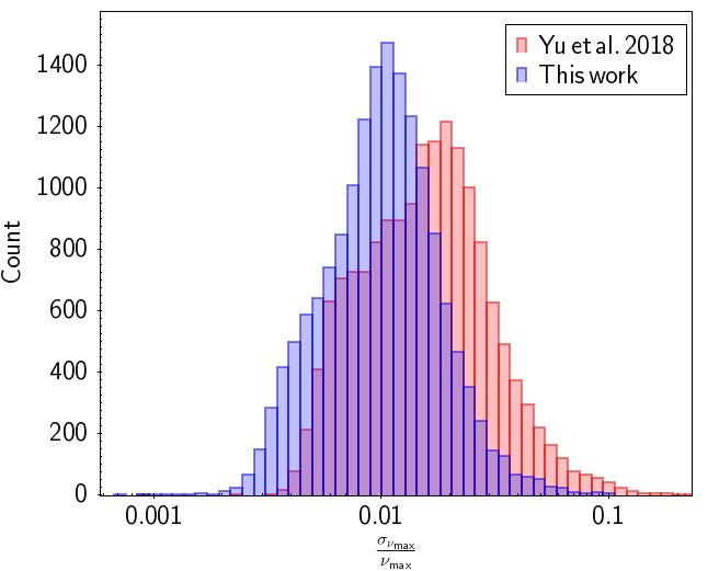
Figure 7: The blue histogram shows the distribution of fractional uncertainty for this work and the light red in the background is the distribution for Yu et al. 2018.

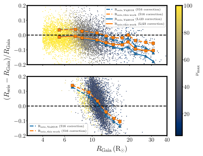
Figure 8: Comparison of radii calculated with $\nu_{\rm max}$ from this work, with radii from Gaia DR2 for $14,794$ stars. The x-axis shows radii from Berger et al. (2018) and y-axis shows fractional difference. The dashed lines shows fractional difference of radii calculated by applying Sharma et al. (2016) correction and the solid lines show the radii calculated using Li et al. (2023). The top panel shows RGB stars and bottom panel shows red clump (RC) stars.

Yu et al. (2018) used the SYD pipeline on the end-of-mission Kepler long-cadence light curves to determine asteroseismic stellar parameters, producing a homogeneous catalogue of $16094$ red giant stars. Their sample was produced from merging six catalogues (Hekker et al., 2011; Huber et al., 2011; Stello et al., 2013; Huber et al., 2014; Mathur et al., 2016; Yu et al., 2016) and limiting their sample to red giants with 5 $\mu$Hz $<$ $\nu_{\rm max}$ $<$ 275 $\mu$Hz.

Figure 5 shows the comparison of our values with Yu et al. (2018). For 97.6 % of stars, the $\nu_{\rm max}$ values from this work agree to within 10%. We found a difference of more than 20% different for 14 stars out of 16094, and we investigated these individually. Of these, KIC 8086924 is actually a long-period variable listed in Yu et al. (2020) with a period of 130.3 d, and does not belong in the Yu et al. (2018) catalogue. For KIC 5775127, strong peaks at 6 $\mu$Hz and 11 $\mu$Hz led to failure of our algorithm. KIC 8645063 and KIC 9284641 were found to be containing two oscillation features in their power spectra, and could be binaries. For KIC 9301329, Yu et al. (2018) determined a $\nu_{\rm max}$ of 191.03 $\mu$Hz and we determined that its correct $\nu_{\rm max}$ is 36.52 $\mu$Hz. The remaining 9 stars failed due to an incorrect initial $\nu_{\rm max}$. This happened because of the unusually high or low mean power level in their power spectrum, contrary to the expected mean power for a star with similar $\nu_{\rm max}$. The correct oscillation parameters for these 8 stars can be obtained by using $\nu_{\rm max,Yu+2018}$ as initial values. Inspection of some of the other outliers in Fig 5 helped us to identify other cases where $\nu_{\rm max,Yu+2018}$ was found to be incorrect, probably due to inadequate modelling of background noise (KIC 6310613 and KIC 5185845). We also found three new stars (KIC 9832790, KIC 4768054 and KIC 6529078) having anomalous peaks.

The bottom panel of Figure 5 shows the fractional difference in the $\nu_{\rm max}$ values between our nuSYD results and the SYD measurements from Yu et al. (2018). The black stars show the median fractional differences for bins of width $10$ $\mu$Hz and we see an offset that is almost constant over most of the range, although it increases towards lower frequencies below 50 $\mu$Hz.

For a given star, the $\nu_{\rm max}$ values between the various different methods are known to span a range of 1–2 % (Hekker et al., 2012; Pinsonneault et al., 2018). These differences presumably arise largely from the different ways each pipeline treats the granulation background and the definition of $\nu_{\rm max}$. This also applies to our nuSYD values, which show an almost constant offset of 1.9 % from SYD (Fig 5). This offset is the same as we found for the solar measurements (Sec. 3.1). Since these two offsets are consistent, it is convenient to use $\nu_{\rm max,\odot}$ from this work to calibrate our $\nu_{\rm max}$ values, in the same way that is done for other pipelines.

To investigate the larger offset at lower $\nu_{\rm max}$ in Figure 5, we split the sample into those on the red giant branch (RGB) and those fusing helium in the core (HeB or Red Clump), based on evolutionary phase from Yu et al. (2018). The RGB stars have an almost constant offset of 2.2 % ($\pm$ 0.03 %) over entire range of $\nu_{\rm max}$ values in the sample, while the RC stars have a much larger offset (4.9$\pm$0.14 %) (see Fig. 6). Even after accounting for the systematic offset compared to solar values, the RC stars have a large departure in $\nu_{\rm max}$ values from this work.

We also compared our uncertainties with those from Yu et al. (2018). In order to measure uncertainties, our nuSYD algorithm was applied to each available quarter of the Kepler light curve, as described in Sec. 2.6, and compared with the fractional uncertainties on $\nu_{\rm max}$ from Yu et al. (2018). The upper panel of Fig. 7 shows the comparison between $\rm\sigma_{\nu_{max,Yu2018}}$ and $\rm\sigma_{\nu_{max,this\,work}}$. The uncertainties in this work (blue bins) have a lower mean value 0.012 ($\pm$ 0.0079) compared to 0.019 ($\pm$ 0.015) of Yu et al. (2018) (orange bins). Since the uncertainties are derived from the quarter-to-quarter scatter, we note that these uncertainties also contain effects due to stochastic nature of solar-like oscillations, and our results imply that $\rm\sigma_{\nu_{max,Yu2018}}$ may be overestimated.

3.3 Comparison with Gaia radii

A simple test to evaluate our $\nu_{\rm max}$ values is to use them to calculate stellar radii and compare these with astrometric stellar radii. We derived stellar radii from the standard scaling relations, using $\nu_{\rm max}$ (and $\rm\nu_{max,\odot}$) from this work, together with $\Delta\nu$ from Yu et al. (2018), corrections to $\Delta\nu$ from theoretical models (Sharma et al., 2016; Stello & Sharma, 2022), and effective temperatures from Berger et al. (2018). We also calculated radii for RGB stars according to Li et al. (2023), which also accounts for the deviations in $\Delta\nu$ due to the so-called surface effect. We then compared these radii with astrometric radii from Berger et al. (2018), who used Gaia DR2 parallaxes—corrected for the zero-point offset (Arenou et al., 2018; Lindegren et al., 2018)—to derive radii for 177,702 Kepler stars.

Figure 8 shows the fractional difference between our radii and those from Berger et al. (2018) for RGB stars (top panel) and RC stars (bottom panel). The orange points show the median values in bins, while the blue points show the same thing when $\nu_{\rm max}$ is taken from Yu et al. (2018). Note that the only difference between the orange and blue curves is in the values of $\nu_{\rm max}$ (and $\rm\nu_{max,\odot}$).

Figure 8 shows systematic offsets between asteroseismic and Gaia radii on the order of about 4 %, which could be due to inaccurate temperature scales, Gaia parallax zero point offsets, or inaccuracies in scaling relations (Huber et al., 2017; Zinn et al., 2019). We observe that radii for RGB stars calculated using $\nu_{\rm max}$ values from this work (orange curve) show a slightly smaller offset from Gaia than using $\nu_{\rm max}$ values from Yu et al. (2018) (blue curve) for more evolved stars ($>15R_{\odot}$). Previous work has demonstrated that asteroseismic scaling relations becomes more inaccurate for more evolved stars (Yu et al., 2020). Therefore, the improved agreement implies that $\nu_{\rm max}$ values from nuSYD yield more accurate asteroseismic radii when compared to a fundamental radius scale from Gaia. For RC stars, we see a similar trend in the fractional difference for SYD and nuSYD. It is interesting that red clump stars seems to show stronger differences between seismic and Gaia radii, which is worthy of further investigation.

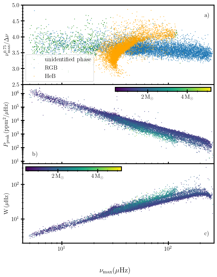
Figure 9: Distribution of various seismic parameters as a function of $\nu_{\rm max}$. In panel a), Green points are the stars whose evolutionary phase is unidentified, Orange points shows the Helium Burning stars and Blue points are RGB stars, using evolutionary phase from Yu et al. (2018). Rest two panels, $P_{\rm peak}$ (panel b) and $W$ (panel c), are colour-coded with stellar mass from Yu et al. (2018).

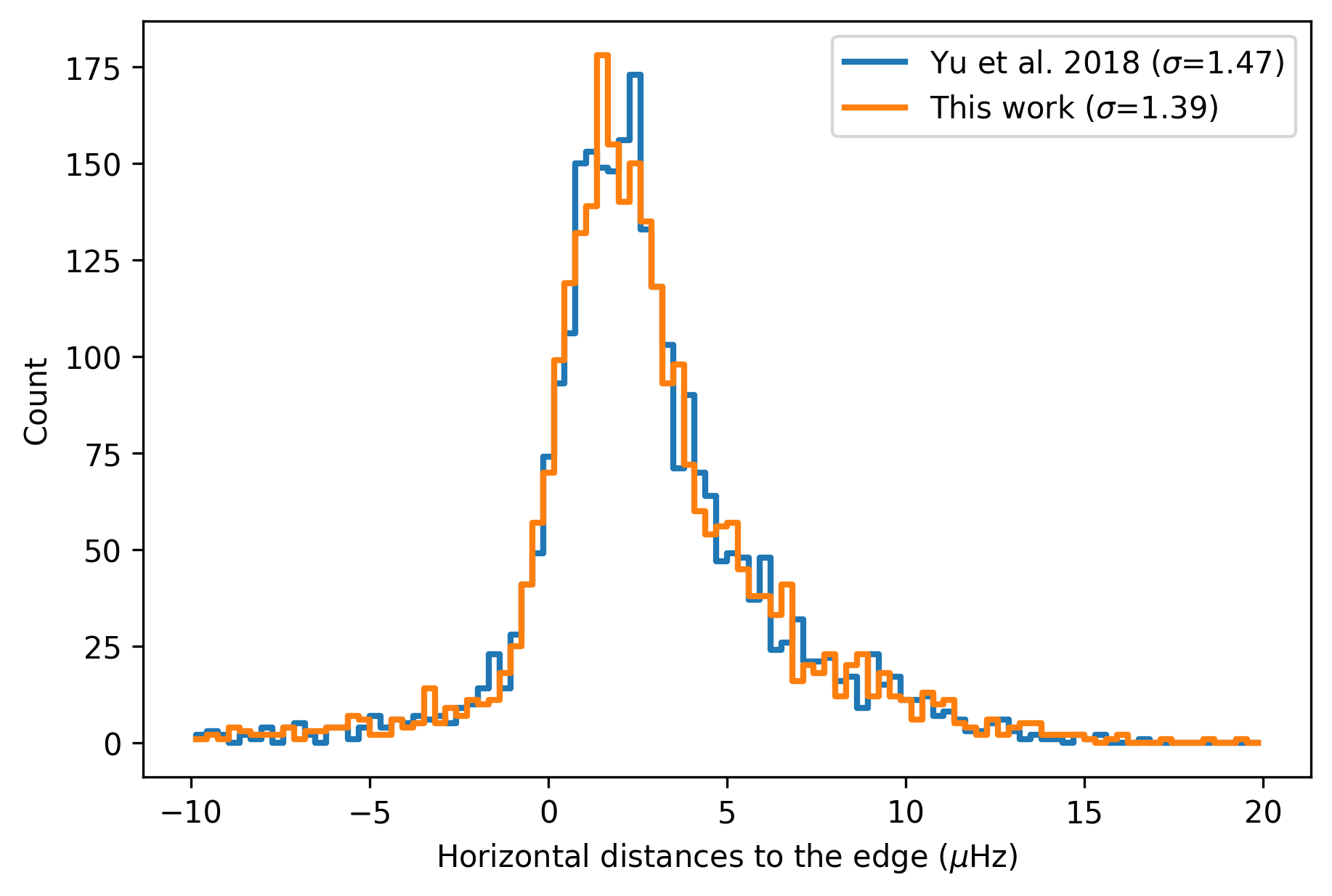
Figure 10: Distribution of scatter in $\nu_{\rm max}$ values from the ZAHeB edge. Blue shows the distances for $\nu_{\rm max}$ values from Yu et al. 2018. Orange ones shows the $\nu_{\rm max}$ values from this work.

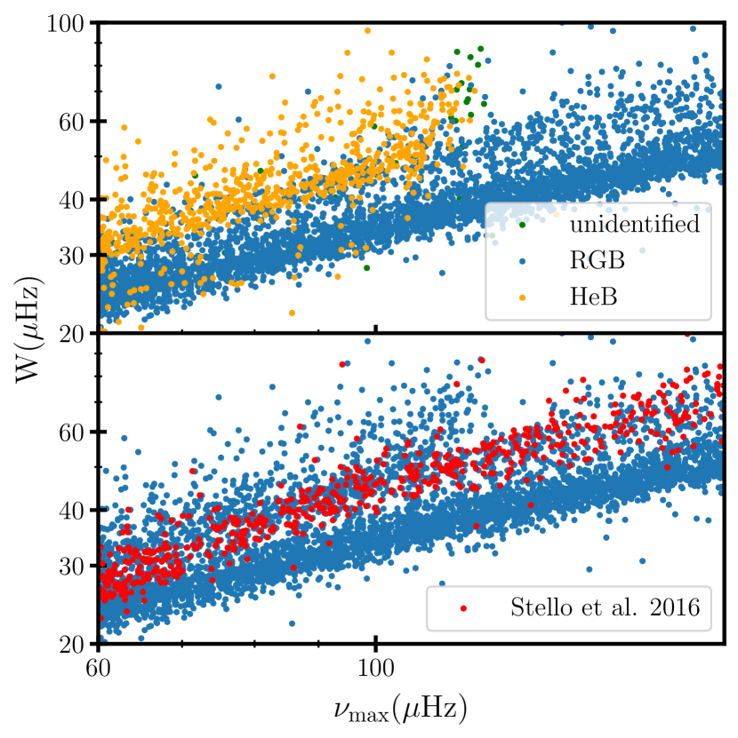
Figure 11: Width of the smoothed envelope, as a function of $\nu_{\rm max}$. Top panel is color coded with evolutionary state from Yu et al. (2018). In bottom panel, the red circles are 730 dipole mode suppressed stars from Stello et al. (2016).

3.4 Analysis of seismic parameters

The measurements for all stars are given in Table 1. Figure 9 shows the various parameters plotted as a function of $\nu_{\rm max}$, all determined using our method. The top panel helps to clearly distinguish stars based on their evolutionary phase (Yu et al., 2018), where the y-axis acts as a proxy for stellar mass. The red clump populations form a distinct, hook-like feature with a sharp edge that corresponds to the zero-age helium burning (ZAHeB) phase (Huber et al., 2010; Bedding et al., 2011; Yu et al., 2018; Li et al., 2022). The slight blurring of this sharp edge is due to the measurement uncertainties of $\Delta\nu$ and $\nu_{\rm max}$, as well as reflecting any intrinsic scatter in the scaling relations (Li et al., 2020). We have checked whether the usage of our $\nu_{\rm max}$ values provides an even sharper edge. To test this, we calculated the horizontal distances of each star from the ZAHeB edge defined in the $\Delta\nu$–$\nu_{\rm max}$ diagram, following the procedures of Li et al. (2020, see their Fig. 6). Figure 10 shows the distributions for $\nu_{\rm max}$ values from this work and Yu et al. (2018), respectively. It can be seen that there is a slight improvement in the sharpness with the $\nu_{\rm max}$ values from this work ($\rm\sigma_{Yu\,et\,al.\,2018}$ = 1.47 and $\rm\sigma_{this\,work}$ = 1.39). In addition, we checked the sharpness of the RGB bump, again using the method of Li et al. (2020), and we found its sharpness is almost identical to earlier results.

Panel b of Fig. 9 shows the peak power ($P_{\rm peak}$) obtained as a function of $\nu_{\rm max}$. This is the sum of oscillation and granulation power, which both follow similar dependencies on $\nu_{\rm max}$. We confirm that this dependence is $P_{\rm peak}\propto\mbox{$\nu_{\rm max}$}{}^{-2.21}$ (Kjeldsen & Bedding, 2011; Mathur et al., 2011). It can be seen that the RC and RGB stars follow different distributions in $P_{\rm peak}$ also (see Fig 7 and 10 of Yu et al. 2018).

The bottom panel of Fig. 9 shows the width of the envelope ($W$) as a function of $\nu_{\rm max}$, which confirms the correlation that has been measured previously, including the tendency for stars at a given $\nu_{\rm max}$ with higher masses to have larger widths (Mosser et al., 2012; Yu et al., 2018; Kim & Chang, 2021). The top panel of Fig. 11 shows a close-up—colour-coded by evolutionary phase—that shows a clear sequence of secondary clump stars, which have higher masses.

We note that our measurements of $W$ tend to be larger than the ‘true’ FWHM of the oscillation envelope because we have not subtracted the granulation background. To see why this is the case, we should recall that FWHM of a distribution is not affected if all the values are multiplied by a constant, but it will be affected if a constant is added to the values. In our case, the oscillation envelope sits on top of a granulation background, which means our measurement of $W$ is greater than the true FWHM of the oscillation envelope. To check this, we compared our width values with those from Yu et al. (2018) and confirmed that our values are overestimated at lower $\nu_{\rm max}$ (by about $40$ %) but are similar (to within $10$ %) at $\nu_{\rm max}$ higher than 70 $\mu$Hz. The similarity for stars with higher $\nu_{\rm max}$ is explained by the fact that their granulation power is comparable to (or less than) the white noise. Since we have measured and subtracted the white noise, our measurement of $W$ for these stars is close to the true FWHM.

The top panel of Fig. 11 also shows that there are two sequences of width values for RGB stars. We identified the upper sequence as stars with suppressed dipole modes (Stello et al., 2016), as shown in the lower panel of Fig. 11. We can explain this using the same argument given in the preceding paragraph. When some modes are suppressed, the amplitude of the oscillation envelope is reduced but the granulation power presumably remains the same. Since the oscillation envelope sits on top of the granulation power, this reduction causes the measured width to be higher than that of a normal star of the same $\nu_{\rm max}$. Once again, our $W$ overestimates the true FWHM of the oscillation envelope, and to an even greater extent due to the weaker oscillations. This suggests that our measurement of $W$ is a simple way to find stars with suppressed dipole modes, without the need to measure the mode visibilities.

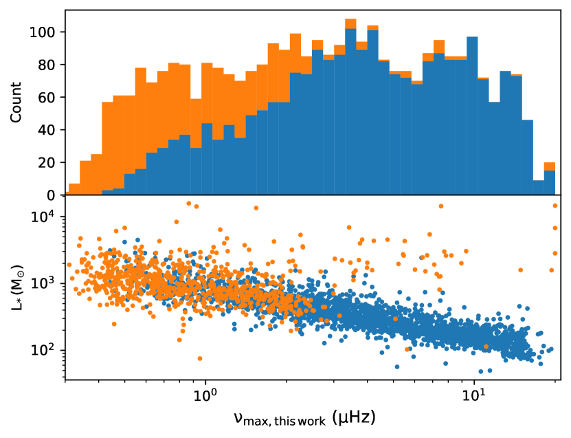
Figure 12: $\nu_{\rm max}$ values (using this method) for the 2336 stars plotted against Gaia DR2 luminosities. $\nu_{\rm max}$ values measured in this work, for stars where $\nu_{\rm max}$ was available (blue) and not reported (orange) in Yu et al. (2020) are shown.

Table 1: Catalogue of measurements for 16094 red giants. The last three columns show our measurements of $\nu_{\rm max}$, $P_{\rm peak}$ and $W$. For convenience, we also include values from Yu et al. (2018) for $\nu_{\rm max,Yu+2018}$, $\rm\Delta\nu$, $\rm T_{eff}$ and evolutionary phase (1 for RGB stars, 2 for HeB stars and 0 for stars with unidentified phase). Only the first 20 entries are shown here; the full table is available online.

KIC	$K_{\rm p}$	quarters	$\rm\nu_{max,Yu+2018}$ ($\rm\mu$Hz)	$\rm\Delta\nu$ ($\rm\mu$Hz)	$T_{\rm eff}$ (K)	Phase	$\rm\nu_{max}$ ($\rm\mu$Hz)	$P_{\rm peak}$ ($\rm ppm^{2}/\mu$Hz)	$W$ ($\rm\mu$Hz)
757137	9.20	17	29.99 $\pm$ 0.60	3.40 $\pm$ 0.01	4751 $\pm$ 139	1	31.00 $\pm$ 0.43	13880 $\pm$ 410	16.65 $\pm$ 0.48
892010	11.67	4	17.85 $\pm$ 0.89	2.43 $\pm$ 0.08	4834 $\pm$ 151	0	18.35 $\pm$ 0.13	61500 $\pm$ 4900	9.00$\pm$ 0.91
892738	11.73	18	7.48 $\pm$ 0.35	1.30 $\pm$ 0.03	4534 $\pm$ 135	0	7.91 $\pm$ 0.12	429600 $\pm$ 27000	4.51 $\pm$ 0.15
892760	13.23	6	29.48 $\pm$ 0.48	3.96$\pm$ 0.12	5188 $\pm$ 183	2	31.12 $\pm$ 1.00	19100 $\pm$ 1800	17.95 $\pm$ 3.57
893214	12.58	15	41.39 $\pm$ 0.54	4.31$\pm$ 0.01	4728 $\pm$ 80	1	41.85 $\pm$ 0.46	6670 $\pm$ 300	20.33 $\pm$ 0.81
893233	11.44	8	6.15 $\pm$ 0.12	1.18 $\pm$ 0.02	4207 $\pm$ 147	0	6.51 $\pm$ 0.14	1000000 $\pm$ 75000	3.63 $\pm$ 0.16
1026084	12.14	15	41.17 $\pm$ 0.90	4.41$\pm$ 0.06	5072 $\pm$ 166	2	48.33 $\pm$ 0.67	3100 $\pm$ 120	27.35 $\pm$ 1.19
1026180	11.74	4	36.91 $\pm$ 0.71	3.99 $\pm$ 0.06	4718 $\pm$ 148	2	36.83 $\pm$ 0.55	15000 $\pm$ 1400	15.72 $\pm$ 0.99
1026309	10.60	18	16.86 $\pm$ 0.76	1.93 $\pm$ 0.03	4514 $\pm$ 80	0	17.54 $\pm$ 0.32	36000 $\pm$ 2300	10.91 $\pm$ 0.50
1026326	13.26	17	94.86 $\pm$ 0.65	8.83 $\pm$ 0.02	5123 $\pm$ 162	1	96.61 $\pm$ 0.41	1500 $\pm$ 54	34.05$\pm$ 1.37
1026452	12.94	18	34.50 $\pm$ 0.52	3.97 $\pm$ 0.08	5089 $\pm$ 154	2	35.67 $\pm$ 0.24	9500 $\pm$ 400	18.36 $\pm$ 0.82
1027110	12.10	18	6.62 $\pm$ 0.19	1.15 $\pm$ 0.02	4190 $\pm$ 80	0	6.78 $\pm$ 0.11	860000 $\pm$ 60000	3.72 $\pm$ 0.17
1027337	12.11	18	74.21 $\pm$ 0.68	6.94 $\pm$ 0.01	4671 $\pm$ 80	1	75.99 $\pm$ 0.54	2800 $\pm$ 100	31.28 $\pm$ 0.84
1027582	13.88	17	157.75 $\pm$ 1.06	12.63 $\pm$ 0.02	5039 $\pm$ 155	1	160.22 $\pm$ 0.58	708 $\pm$ 39	45.19 $\pm$ 1.62
1028267	13.28	8	103.13 $\pm$ 0.83	9.47 $\pm$ 0.02	5242$\pm$ 183	1	106.30 $\pm$ 0.80	1301 $\pm$ 48	39.43 $\pm$ 1.68
1160684	14.91	17	26.38 $\pm$ 0.97	3.36$\pm$ 0.22	4128 $\pm$ 128	2	28.29 $\pm$ 0.32	17700 $\pm$ 1100	15.29 $\pm$ 0.51
1160789	9.70	18	24.72 $\pm$ 0.62	3.51 $\pm$ 0.05	4724 $\pm$ 80	2	26.23 $\pm$ 0.31	28700 $\pm$ 940	15.58 $\pm$ 0.45
1161447	12.61	7	36.18 $\pm$ 1.55	4.12$\pm$ 0.06	4793 $\pm$ 80	2	39.11 $\pm$ 0.41	9500 $\pm$ 700	20.34 $\pm$ 0.83
1161618	10.22	18	34.32 $\pm$ 0.50	4.11 $\pm$ 0.03	4747 $\pm$ 80	2	35.44 $\pm$ 0.46	14900 $\pm$ 740	18.17 $\pm$ 1.12
1162220	11.22	18	11.00 $\pm$ 0.32	1.67 $\pm$ 0.02	4218 $\pm$ 80	1	11.50 $\pm$ 0.17	248000 $\pm$ 15000	6.42 $\pm$ 0.26

3.5 Application to Long Period Variables

We also tested the algorithm on stars that have a lower range of $\nu_{\rm max}$ values. Yu et al. (2020) studied 3213 Kepler high-luminosity red giants with pulsation periods greater than 0.6 d ($\mbox{$\nu_{\rm max}$}<18.35$ $\mu$Hz). They used 4 years of Kepler light curves and Gaia DR2 parallaxes to compare asteroseismic and astrometric radii. They measured $\nu_{\rm max}$ using the SYD pipeline for 2336 stars with highest $\nu_{\rm max}$ as 18 $\mu$Hz. In order to check whether our pipeline is able to measure oscillations at very low $\nu_{\rm max}$, we applied our algorithm to these 2336 stars. Note that we calculated $\rm P_{stellar}$ above 0.1 $\mu$Hz instead of 5 $\mu$Hz for the initial $\nu_{\rm max}$(see sec 2.2), as we expect very low $\nu_{\rm max}$ values. Also, we did not apply any high-pass filtering to the light curves. Figure 12 shows the results from the application of our method on the sample. The blue histogram shows the $\nu_{\rm max}$ values for 2336 stars which already had $\nu_{\rm max}$ values in Yu et al. (2020) and orange histogram shows $\nu_{\rm max}$ values measured in this work for the additional 857 stars, which does not have a $\nu_{\rm max}$ value in Yu et al. (2020). A visual inspection of the outliers in orange points shows stars that have sections in the light curve with very large scatter, for which our algorithm failed to identify the region of oscillation. For 98 % of the stars, our $\nu_{\rm max}$ values follow the luminosity-$\nu_{\rm max}$ relation (Yu et al., 2020). Hence, this is a good demonstration that this method is able to measure oscillations in low $\nu_{\rm max}$ stars, without any prior information.

4 Conclusions

Here we demonstrate a simple, data-driven method to measure $\nu_{\rm max}$ by smoothing the power spectra. Our method is able to detect oscillations in 99.91 % of Kepler red giants in Yu et al. (2018) and measure their properties. It only took 50 minutes to return all parameters for 16094 stars on a 13th Gen Intel® Core™ i7-13700H 14-core laptop. Hence we find that it is fast, simple and works well for stars with a wide range of oscillation properties. The measurements for all stars are given in Table 1. Following are our conclusions from this work.

• The $\nu_{\rm max}$ values show agreement with Yu et al. (2018), but with a systematic offset that we calibrate by applying the same method to observations of the solar oscillations. For RGB stars, this offset is within 2.2 % and for RC stars this offset is around 4.8 %. Since the difference between Yu et al. (2018) and this work is in the way the granulation background is treated, and considering that this offset depends upon evolutionary states, this difference in offset may hint at difference in manifestation of granulation background between evolutionary states.

• Further we compared the radii calculated using scaling relations with Gaia radii and found that the seismic radii calculated using $\nu_{\rm max}$ values from this work mimic the general trend as observed in (Zinn et al., 2019, 2023). Further, the radii from this work have a constant offset relative to Gaia radii, whereas the previous results become greater for more evolved stars.

• We also estimated the uncertainties on $\nu_{\rm max}$ ($\rm\sigma_{\nu_{max}}$) by applying our method on each quarter of Kepler light curves of 16094 red giants, with mean uncertainties around 1.2 %. For short light curves, one way to estimate uncertainties would be trying to derive a global relation that connects $\rm\sigma_{\nu_{max}}$ with the measured quantities. Another way to derive more realistic uncertainties would be by random sampling (bootstrapping) the time series or power spectra (Huber et al., 2009; Chontos et al., 2021).

• We also reproduced some results from Yu et al. (2018), using the $\nu_{\rm max}$, $P_{\rm peak}$ and $W$ measured in this work. It is interesting to note that the $\nu_{\rm max}$ values from this work sharpens the ZAHeB edge. This suggests that $\nu_{\rm max}$ values from this work help to differentiate stars on ZAHeB edge. Also, one new result is that our $W$ can clearly identify the dipole mode suppressed stars as a distinct population.

• We also applied this method to low $\nu_{\rm max}$ stars in (Yu et al., 2020). The method was successful in measuring $\nu_{\rm max}$ values as low as 0.19 $\mu$Hz. We also applied this method to a few low S/N stars like KIC 9236658 and KIC 6698391, and is able to measure oscillations and hence other parameters. This shows the flexibility of the method.

With large amount of photometric data available from space missions, the demonstrated method would be able to measure oscillations quickly. Next, we plan to apply this method to TESS observations of the the Kepler red giants (Stello et al., 2022), and then to a much larger sample of TESS stars.

Data Availability

The Kepler data underlying this article are available at the MAST Portal (Barbara A. Mikulski Archive for Space Telescopes), at https://mast.stsci.edu/portal/Mashup/Clients/Mast/Portal.html

References

- Arenou et al. (2018) Arenou F., et al., 2018, A&A, 616, A17
- Astropy Collaboration (2013) Astropy Collaboration 2013, A&A, 558, A33
- Astropy Collaboration (2018) Astropy Collaboration 2018, AJ, 156, 123
- Basri et al. (2010) Basri G., et al., 2010, ApJ, 713, L155
- Bedding & Kjeldsen (2003) Bedding T. R., Kjeldsen H., 2003, Publ. Astron. Soc. Australia, 20, 203
- Bedding et al. (2011) Bedding T. R., et al., 2011, Nature, 471, 608
- Belkacem et al. (2011) Belkacem K., Goupil M. J., Dupret M. A., Samadi R., Baudin F., Noels A., Mosser B., 2011, A&A, 530, A142
- Bell et al. (2019) Bell K. J., Hekker S., Kuszlewicz J. S., 2019, MNRAS, 482, 616
- Berger et al. (2018) Berger T. A., Huber D., Gaidos E., van Saders J. L., 2018, The Astrophysical Journal, 866, 99
- Brown et al. (1991) Brown T. M., Gilliland R. L., Noyes R. W., Ramsey L. W., 1991, ApJ, 368, 599
- Bugnet et al. (2018) Bugnet L., García R. A., Davies G. R., Mathur S., Corsaro E., Hall O. J., Rendle B. M., 2018, A&A, 620, A38
- Chaplin & Miglio (2013) Chaplin W. J., Miglio A., 2013, ARA&A, 51, 353
- Chaplin et al. (2011) Chaplin W. J., et al., 2011, The Astrophysical Journal, 732, 54
- Chontos et al. (2021) Chontos A., Huber D., Sayeed M., Yamsiri P., 2021, pySYD: Measuring global asteroseismic parameters, Astrophysics Source Code Library, record ascl:2111.017 (ascl:2111.017)
- Colman et al. (2017) Colman I. L., et al., 2017, MNRAS, 469, 3802
- Fröhlich et al. (1995) Fröhlich C., et al., 1995, Sol. Phys., 162, 101
- Gehan et al. (2023) Gehan C., Campante T. L., Cunha M. S., Pereira F., 2023, Astronomische Nachrichten, 344, easna.20220090
- Gilliland et al. (2010) Gilliland R. L., et al., 2010, The Astrophysical Journal Letters, 713, L160
- Harris et al. (2020) Harris C. R., et al., 2020, Nature, 585, 357
- Harvey (1985) Harvey J., 1985, in Rolfe E., Battrick B., eds, ESA Special Publication Vol. 235, Future Missions in Solar, Heliospheric & Space Plasma Physics. p. 199
- Hekker (2020) Hekker S., 2020, Frontiers in Astronomy and Space Sciences, 7, 3
- Hekker et al. (2010) Hekker S., et al., 2010, Monthly Notices of the Royal Astronomical Society, 402, 2049
- Hekker et al. (2011) Hekker S., et al., 2011, Monthly Notices of the Royal Astronomical Society, 414, 2594
- Hekker et al. (2012) Hekker S., et al., 2012, A&A, 544, A90
- Hon et al. (2018) Hon M., Stello D., Zinn J. C., 2018, ApJ, 859, 64
- Hon et al. (2019) Hon M., Stello D., García R. A., Mathur S., Sharma S., Colman I. L., Bugnet L., 2019, MNRAS, 485, 5616
- Hon et al. (2021) Hon M., et al., 2021, ApJ, 919, 131
- Howe et al. (2020) Howe R., et al., 2020, MNRAS, 493, L49
- Huber et al. (2009) Huber D., Stello D., Bedding T. R., Chaplin W. J., Arentoft T., Quirion P. O., Kjeldsen H., 2009, Communications in Asteroseismology, 160, 74
- Huber et al. (2010) Huber D., et al., 2010, The Astrophysical Journal, 723, 1607
- Huber et al. (2011) Huber D., et al., 2011, The Astrophysical Journal, 743, 143
- Huber et al. (2014) Huber D., et al., 2014, The Astrophysical Journal Supplement Series, 211, 2
- Huber et al. (2017) Huber D., et al., 2017, The Astrophysical Journal, 844, 102
- Hunter (2007) Hunter J. D., 2007, Computing in Science & Engineering, 9, 90
- Jackiewicz (2021) Jackiewicz J., 2021, Frontiers in Astronomy and Space Sciences, 7
- Jenkins et al. (2010) Jenkins J. M., et al., 2010, ApJ, 713, L120
- Kallinger et al. (2010) Kallinger T., et al., 2010, A&A, 522, A1
- Kallinger et al. (2014) Kallinger T., et al., 2014, A&A, 570, A41
- Kallinger et al. (2016) Kallinger T., Hekker S., Garcia R. A., Huber D., Matthews J. M., 2016, Science Advances, 2, 1500654
- Kim & Chang (2021) Kim K.-B., Chang H.-Y., 2021, New Astron., 84, 101522
- Kim & Chang (2022) Kim K.-B., Chang H.-Y., 2022, New Astron., 92, 101720
- Kjeldsen & Bedding (1995) Kjeldsen H., Bedding T. R., 1995, A&A, 293, 87
- Kjeldsen & Bedding (2011) Kjeldsen H., Bedding T. R., 2011, A&A, 529, L8
- Kjeldsen et al. (2005) Kjeldsen H., et al., 2005, The Astrophysical Journal, 635, 1281
- Li et al. (2020) Li Y., Bedding T. R., Stello D., Sharma S., Huber D., Murphy S. J., 2020, Monthly Notices of the Royal Astronomical Society, 501, 3162
- Li et al. (2022) Li Y., et al., 2022, Nature Astronomy, 6, 673
- Li et al. (2023) Li Y., et al., 2023, Monthly Notices of the Royal Astronomical Society, 523, 916
- Lightkurve Collaboration et al. (2018) Lightkurve Collaboration et al., 2018, Lightkurve: Kepler and TESS time series analysis in Python, Astrophysics Source Code Library (ascl:1812.013)
- Lindegren et al. (2018) Lindegren L., et al., 2018, A&A, 616, A2
- Mathur et al. (2010) Mathur S., et al., 2010, A&A, 511, A46
- Mathur et al. (2011) Mathur S., et al., 2011, The Astrophysical Journal, 741, 119
- Mathur et al. (2016) Mathur S., García R. A., Huber D., Regulo C., Stello D., Beck P. G., Houmani K., Salabert D., 2016, The Astrophysical Journal, 833, 294
- Miglio et al. (2012) Miglio A., et al., 2012, MNRAS, 419, 2077
- Mosser & Appourchaux (2009) Mosser B., Appourchaux T., 2009, A&A, 508, 877
- Mosser et al. (2012) Mosser B., et al., 2012, A&A, 537, A30
- Pande et al. (2018) Pande D., Bedding T. R., Huber D., Kjeldsen H., 2018, MNRAS, 480, 467
- Pinsonneault et al. (2018) Pinsonneault M. H., et al., 2018, The Astrophysical Journal Supplement Series, 239, 32
- Salabert et al. (2017) Salabert D., García R. A., Jiménez A., Bertello L., Corsaro E., Pallé P. L., 2017, A&A, 608, A87
- Sharma et al. (2016) Sharma S., Stello D., Bland-Hawthorn J., Huber D., Bedding T. R., 2016, The Astrophysical Journal, 822, 15
- Smith et al. (2012) Smith J. C., et al., 2012, PASP, 124, 1000
- Stello & Sharma (2022) Stello D., Sharma S., 2022, Research Notes of the AAS, 6, 168
- Stello et al. (2009) Stello D., Chaplin W. J., Basu S., Elsworth Y., Bedding T. R., 2009, MNRAS, 400, L80
- Stello et al. (2013) Stello D., et al., 2013, The Astrophysical Journal Letters, 765, L41
- Stello et al. (2016) Stello D., Cantiello M., Fuller J., Huber D., García R. A., Bedding T. R., Bildsten L., Silva Aguirre V., 2016, Nature, 529, 364
- Stello et al. (2022) Stello D., et al., 2022, MNRAS, 512, 1677
- Stumpe et al. (2012) Stumpe M. C., et al., 2012, PASP, 124, 985
- Virtanen et al. (2020) Virtanen P., et al., 2020, Nature Methods, 17, 261
- Yu et al. (2016) Yu J., Huber D., Bedding T. R., Stello D., Murphy S. J., Xiang M., Bi S., Li T., 2016, Monthly Notices of the Royal Astronomical Society, 463, 1297
- Yu et al. (2018) Yu J., Huber D., Bedding T. R., Stello D., Hon M., Murphy S. J., Khanna S., 2018, ApJS, 236, 42
- Yu et al. (2020) Yu J., Bedding T. R., Stello D., Huber D., Compton D. L., Gizon L., Hekker S., 2020, MNRAS, 493, 1388
- Zinn et al. (2019) Zinn J. C., Pinsonneault M. H., Huber D., Stello D., Stassun K., Serenelli A., 2019, The Astrophysical Journal, 885, 166
- Zinn et al. (2023) Zinn J. C., Pinsonneault M. H., Bildsten L., Stello D., 2023, MNRAS, 525, 5540