Unraveling Variability and Estimating Mass Loss
of Exoplanets in the Triplet Star System LTT 1445

Abstract

Context. The high-energy environment of the host stars could be deleterious for their planets. It is crucial to ascertain this contextual information to fully characterize the atmospheres of terrestrial exoplanets.

Aims. We aim to fully characterize a unique triple system, LTT1445, with three known rocky exoplanets around LTT 1445A.

Methods. The X-ray irradiation and flaring of this system are studied through a new 50 ks Chandra observation, which is divided into 10 ks, 10 ks, and 30 ks segments conducted two days apart, and two months apart, respectively. This is complemented by an archival Chandra observation approximately one year earlier and repeated observations with eROSITA (extended ROentgen Survey with an Imaging Telescope Array), the soft X-ray instrument on the Spectrum-Roentgen-Gamma (SRG) mission, enabling the investigation of X-ray flux behavior across multiple time scales. The flux data acquired from these observations serve as a basis for estimating the photo-evaporation mass loss of the individual exoplanets with their host stars. To gain deeper insights into the environmental context influenced by XUV flux and to better understand the anticipated atmospheric conditions of the planets orbiting the A component, we integrate the use of the planet modeling package, VPLanet.

Results. Our findings indicate that LTT 1445C is the primary contributor to X-ray emissions, with additional input from LTT 1445B. Moreover, our study confirms that LTT 1445A, recognized as a slowly-rotating star, exhibits no significant flare activity in the observed dataset. The observed results also suggest that the X-ray emissions from the LTT 1445BC components do not pose a greater threat to the planets orbiting LTT 1445A than the emissions from A itself. According to simulation results, LTT 1445Ad might have the capacity to retain its water surface.

1 Introduction

Exoplanet science is entering a new phase focused on characterizing exoplanet atmospheres and identifying potentially habitable planets. This goal is currently attainable through spectroscopic analysis of nearby terrestrial exoplanets around mid to late M dwarfs, particularly those with slow rotation, relatively low activity, and masses ranging from 0.10 to 0.25 Earth masses (Morley et al., 2017; National Academies of Sciences, 2018). However, caution must be exercised when characterizing potentially habitable planets due to the potential impact of the host star’s high-energy environment on their atmospheres.

Exoplanets orbiting M dwarfs are prime targets for characterizing the habitability of other worlds (Shields et al., 2016) because they are abundant (Bochanski et al., 2010) within their closed-in habitable zone (HZ) (Kasting et al., 1993; Kopparapu et al., 2013). Population studies (e.g., Dressing & Charbonneau, 2015) estimate that, on average, for every seven M dwarfs, the orbit of at least one Earth-size planet is in the HZ. So far, numerous exoplanets with a rocky composition have been detected. A significant proportion of these rocky planets is found near M-type stars. However, the proximity of these planets to their host stars can pose potential hazards to their physical and chemical characteristics. Exoplanets close to M dwarfs are potentially exposed to high levels of X-ray and extreme ultraviolet radiation (XUV) and strong particle fluxes from stellar winds or coronal mass ejections (Lammer et al., 2011). On average, two-thirds of these cool stars are active, according to a survey of 238 nearby M dwarfs from Earth (West et al., 2015). Many studies consider XUV radiation from M dwarfs as deleterious for life (Heath et al., 1999; Tarter et al., 2007; Lammer et al., 2009; Shields et al., 2016; Meadows et al., 2018).

To assess habitability and comprehend the planetary atmospheric escape mechanisms contributing to planetary mass loss and oxygen accumulation, it is vital to analyze the high-energy environment of M dwarfs. This involves examining stellar activity, variability, and flare frequency. For comparison, while the Sun emits the most energetic flares at an energy level of $\mathrm{10^{32}\,erg}$ once per solar cycle (Youngblood et al., 2017), M dwarfs can experience flares of the same energy level every day (Audard et al., 2000). Moreover, even flares from inactive stars could affect the chemistry of the atmospheres of orbiting planets (Hawley et al., 2014).

In the context of the rotation-activity relation, Skumanich (1972) established an empirical link between a star’s rotation rate and its age, stating that the equatorial speed of a star decreases as the inverse square root of its age within the range of 100 Myr to 10 Gyr. Pallavicini et al. (1981) later identified a correlation between rotation and activity, expressing X-ray brightness as $L_{x}(v\sin i)^{1.9}$, providing initial evidence of dynamo-induced stellar coronal activity. For fast rotators, this relationship saturates at $\mathrm{L_{x}/L_{bol}=10^{-3}}$ (Micela et al., 1985). The X-ray-rotation relation for slow rotators is sparsely populated, posing challenges in accurately determining its turnover point and slope. Stelzer et al. (2016) used X-ray data to incorporate UV emission as a diagnostic for chromospheric activity in field M stars, deriving a saturation level of $\mathrm{LogL_{x,sat}=28.6\pm 0.3\,erg/s}$ for M3-M4 stars with $\mathrm{P_{rot}}$ ¡ 10 days. Wright et al. (2011) analyzed 824 solar and late-type stars, introducing the Rossby number (Ro) as an evaluation of the convective turnover time. It revealed saturated and unsaturated phases at a Rossby number of approximately 0.13. Wright et al. (2018) later expanded the sample to include 19 slowly rotating fully convective stars, suggesting that both fully- and partly- convective stars operate similar dynamos, relying on the interplay of rotation and turbulent convection.

Table 1: The three stars in the LTT 1445 system

Star	Spectral	$M_{*}^{b}$	$R_{*}^{b}$	$L_{bol}^{b}$
	Typea,b	[$M_{{\odot}}$]	[$R_{{\odot}}$]	[$10^{31}\,erg/s$]
A	M 3	0.257$\pm$0.014	0.268$\pm$0.027	3.04
B	M 3.5	0.215 $\pm$ 0.014	0.236$\pm$0.027	2.28
C	M 4	0.161 $\pm$ 0.014	0.197$\pm$0.027	1.41

• Reference ^a Reid et al. (2004); ^b Winters et al. (2019) .

A closest transiting exoplanetary system to us is LTT 1445, a triplet star system with three rocky exoplanets (Winters et al., 2019, 2022; Lavie et al., 2022) around the A component. The LTT 1445 system, located 6.9 parsecs away from the Sun, consists of three low-mass M-type stars: A, and a binary pair, B and C. This stellar system denoted as ABC, has parameters shown in Table 1. According to Reid et al. (2004) and Winters et al. (2019), the spectral type of star A in the LTT 1445 system is classified as M3. Stars B and C are classified as M3.5 and M4, respectively. The separation between LTT 1445A and LTT 1445BC is 34 astronomical units (AU) or approximately 7” on the sky (Winters et al., 2019; Brown et al., 2022), with an orbital period of 250 years. The B and C components orbit each other with a period of 36 years, and are separated by 1.25” on the sky (Brown et al., 2022). Ground-based MEarth observations have shown in the image that the BC pair is always blended, while the blending between A and BC is variable (Winters et al., 2022).

Previous observations have documented stellar activity in the LTT 1445 system. The TESS light curve revealed stellar flares and rotational modulation attributed to star spots, likely originating from either or both of the B or C components (Winters et al., 2019). A super-flare with an energy of $\mathrm{10^{34}\,erg}$ was also observed (Howard et al., 2019). Subsequently, the system was detected by eROSITA in the first eROSITA all-sky survey (eRASS1), where it was assumed that all the detected flux originated from the known active stars in BC (Foster et al., 2022). Brown et al. (2022) revealed a wide range of variability in the A component from the 30ks Chandra observation conducted in 2021. This suggests highly fluctuating and stochastic high-energy irradiance on its planets, leading to potential atmospheric alterations. Leveraging the high spatial resolution of Chandra, Brown et al. (2022) resolved all three components and reported the X-ray flux from the A flare at a level of $3.61\pm 0.27\times\mathrm{10^{-13}\,ergcm^{-2}s^{-1}}$, while the BC flare emitted $20.2\pm 0.9\times\mathrm{10^{-13}\,ergcm^{-2}s^{-1}}$. The quiescent X-ray luminosity for the A component was reported at the low level of $3.7\times\mathrm{10^{25}\,ergs^{-1}}$.

Renowned for its proximity and the brightness of its stars, the LTT1445 system stands out as a promising candidate for in-depth planet characterization. In the literature, XUV flux around LTT 1445, or PMI03018-1635, was explored by Stelzer et al. (2013), who combined archival ROSAT, XMM–Newton, and GALEX data for the BC component, measuring the X-ray flux in the 0.2-2.0 keV energy band with $\log F_{x}/\mathrm{mW/m^{2}}$ equal to 12.06. Despite these insights, several questions remain from the Brown et al. (2022) analysis of their Chandra data, including whether LTT 1445B was observed during quiescence, the rotational characteristics of the B component, and the potential influence of BC activity on planets around the A component.

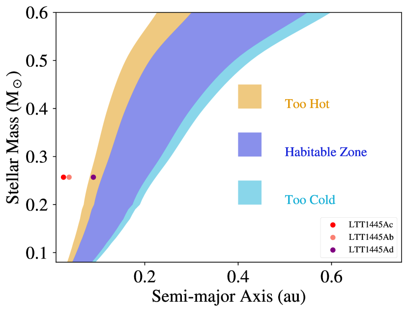
Figure 1: The positions of each planet relative to the host star LTT1445A were computed following Kopparapu et al. (2013), assuming the stellar age to be 0.18 Gyr. The Habitable Zone is the distance from the star where a liquid water layer is sustained. This model evaluates the habitability potential of extrasolar terrestrial planets by suggesting the use of stellar flux incident on a planet instead of equilibrium temperature. This eliminates the dependency on planetary albedo, which varies based on the spectral type of the host star.

Rocky Planets in Triple Star System

The star LTT 1445A hosts three rocky exoplanets. The detection of the initial two planets involved the analysis of photometric data from various sources, including MEarth, Las Cumbres Observatory Global Telescope (LCOGT), and Transiting Exoplanet Survey Satellite (TESS), to detect transits. To further characterize these exoplanets, spectroscopic data from 136 radial velocities (RV) of LTT 1445A were collected over two years using high-resolution spectrographs.

Detailed information about the planetary parameters of the LTT 1445 system can be found in Table 2. Winters et al. (2022) precisely measured the masses of both planets, and the mass-radius relation, based on the interior structure model (Zeng & Sasselov, 2013), indicated an Earth-like composition with approximately 33% iron and 67% rock. Subsequently, Lavie et al. (2022) utilized 84 the Echelle SPectrograph for Rocky Exoplanets and Stable Spectroscopic Observations (ESPRESSO) high-resolution spectra and nested sampling algorithm Buchner et al. (2014), a reliable statistical method Nelson et al. (2020) of discovering LTT 1445Ad, which orbits at the inner boundary of the habitable zone of its host. Here, we estimate the radius of this planet to be 1.29 $R_{\oplus}$ based on the mass-radius prediction in Fig. 3 of Chen & Kipping (2017). The positions of the three planets relative to the host star are illustrated in Fig. 1.

Table 2: The three rocky exoplanet companions of LTT 1445A

Planet	$M_{P}$	$R_{P}$	a	$P$
	[$M_{{\oplus}}$]	[$R_{{\oplus}}$]	[AU]	[days]
cd	$1.54^{+0.20}_{-0.19}$	$>1.147^{+0.055}_{-0.0054}$	$0.02656$	3.12390
bc	$2.87^{+0.26}_{-0.25}$	$1.305^{+0.067}_{-0.060}$	$0.03807$	5.35877
de	$2.72\pm 0.75$	non-transiting*	0.09	24.30388

• Reference ^c Winters et al. (2022); ^d Winters et al. (2019); ^e Lavie et al. (2022) , *estimated 1.29$R_{\oplus}$.

This study revisits the LTT 1445 triplet star system with new Chandra and eROSITA data, primarily focusing on the analysis of X-ray observations from the host stars, LTT 1445A and LTT 1445BC (Section 2).

The methodology is described in Section 3. Our comprehensive analysis includes the examination of the variability in X-ray flux emitted by these stars, using data collected over 3 years from both eROSITA and Chandra observatories (Section 4). Additionally, we estimate various parameters related to the activity level, mass loss rate, and mass loss evolution of each planet within the system. In Section 5, we delve into the phenomenon of oxygen build-up and discuss its implications within the context of LTT 1445. The summary is provided in Section 6.

2 Observations

2.1 Chandra Observations

Chandra ACIS-S observations, totaling 50 ks, were granted as part of MPE GTO time (proposal 23100661 cycle 23). This system revisit occurred approximately 1.5 years after the Chandra observation reported by Brown et al. (2022). Our observations were divided into three epochs. The first and second observations were taken 2 days apart, while the last observation occurred 1.5 months after the first one. The observation log is detailed in Table 3. Benefiting from Chandra’s high spatial resolution, we are able to analyse the components of LTT1445, namely A and BC, separately.

Table 3: Chandra Observation log

Obs ID	Instrument	Dur.(s)	Obs.time
25993	Chandra ACIS	11000	2022-10-10T09:08:22
27476	Chandra ACIS	10000	2022-10-12T08:38:48
27477	Chandra ACIS	29000	2022-11-22T23:38:24

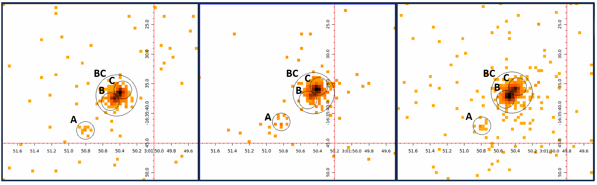
Figure 2: Chandra/ACIS image of the LTT 1445 system for the three observations. North is up, east is left. The black circles show the photon extraction region from the three Chandra observations: 2022-10-10, 2022-10-12 and 2022-11-24 (left to right) for each component A, B, C, and BC together.

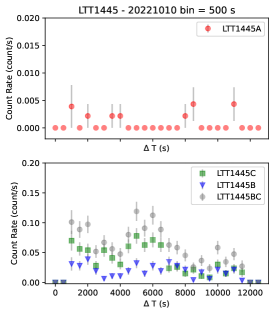
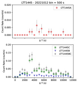
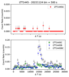
Figure 3: Light curves extracted from the three Chandra observations: 2022-10-10, 2022-10-12 and 2022-11-24 (left to right) of the A component (red, top panels), B in green square, C in blue triangle and combined BC in gray diamond (bottom panels).

The collected data were analyzed following standard procedures outlined in the CIAO package version 4.14, as detailed by Fruscione et al. (2006). In our analysis, the event list was filtered to the 0.3-10 keV energy range. Circular regions with a radius of 1.5” were applied for source data extraction for each of the three components: LTT 1445 A, B, and C. Larger circular regions with a radius of 3” were employed for the combined BC components, and the background region was defined as an annulus.

We jointly extract data from BC to analyze the flux and assess potential impacts on the planets orbiting the A component. Additionally, we extract each star individually, to discern the activity level of each star. The three star components are aligned in a northeast-to-southwest direction, with the projected distance from A to B being approximately 7” as shown in Fig.2.

In the region corresponding to the A component in Fig. 2, the counts detected in each observation from Table 3 were 9, 11, and 12 counts. For the region of B, we recorded counts of 194, 81, and 598 for each respective observation. Regarding C’s region, the counts detected were 381, 335, and 391 for the three observations.

After identifying the source locations, we extracted the light curve from each component. The light curves, with a bin size of 500 seconds for each dataset, are presented in Fig. 3. Regarding LTT1445A, its stellar variability remained relatively quiet across all three datasets, as indicated by the top panel in red at a level of 0.005 counts/second. For LTT1445BC, the initial two datasets on the left were captured within two days. Both components exhibit a comparable activity level; B is in a quiet period with an average of 0.03 counts/second, while C is considered quasi-quiescent (qq) or elevated at a level of 0.05 counts/second. The bottom-left panel does not display prominent flare characteristics; instead, it exhibits quasi-quiescent behavior.

In the middle panel of Fig. 3, a flare event was observed in component C at a level of 0.10 counts/second. The last dataset, collected approximately 1.5 months later, distinctly demonstrates the variability of this system, with a flare predominantly originating from component B at a level of 0.15 counts/second. These observing time intervals reveal the energy transfer dynamics within the binary system.

We study the stellar spectrum of each component during both quiescence and flaring. To achieve this, we segmented the X-ray light curves of the A and BC components into distinct time intervals, classifying them as either quiescent (or quasi-quiescent, qq) or during flares. Subsequently, we extracted the spectrum of each component during the qq and flare time intervals. For the new 50 ks Chandra observation, our spectrum extraction followed the standard routine from CIAO. Regions of interest for the three stars, as depicted in Fig. 2, were assigned, along with an annulus background region sufficiently large to encompass the background around the source ABC. Subsequently, light curves were generated following the method described in Section 2.1, and flare intervals were identified for BC components based on the light curves in Fig. 3 and are detailed in Table 4. As the A component remained quiet in all datasets, we present data only for the BC components during each identified interval. We later combined corresponding intervals (e.g., Flare) from all three datasets for spectral extraction. The specextract script was applied to create source and background spectra from Chandra imaging mode, which were subsequently employed in spectral modeling.

Table 4: Flare interval identification for BC components from the Chandra observation in 2022

Obs.date	Intervals	Duration [s]
2022-10-10	QQ	0-12000
2022-10-12	Quiet	0-1800
	Flare	1800-4000
	QQ	4000-12000
2022-11-24	Quiet	0-14000
	Flare	14000-18000
	QQ	18000-30000

2.2 eROSITA Observations

The eROSITA all-sky survey (eRASS; Predehl et al., 2021), started in 2019, and passed over LTT1445 four times: eRASS1 (Merloni et al., 2024) on 2020-01-25, eRASS2 on 2020-07-26, eRASS3 on 2021-01-19, eRASS4 on 2021-07-27), with gaps of 6 months. The initial Chandra observation in June 2021 (Brown et al., 2022) lies between eRASS3 and eRASS4.

In this study, we leverage sources detected in the 0.2–2.3 keV range from eRASS1 to eRASS4 for continuous system monitoring. Specifically, we use the eRASS1 to eRASS4 source catalog versions 221031, 230619, and 230119 processed by the eSASS pipeline version 020 (Brunner et al., 2022).

3 Method

In this section, we describe the methodologies used in spectral analysis, including our spectral model in Section 3.2 and the adopted statistical approach in Section 3.1. Furthermore, we explain the model for X-ray-driven atmospheric escape used to understand the impact on the planets in Section 3.3.

3.1 Statistical Method

In X-ray astronomy, the chi-square statistic ($\mathrm{\chi^{2}}$) and C-statistic (Cstat) (Cash, 1979) are commonly used in spectral fitting. These differ in assumptions and applications. The $\mathrm{\chi^{2}}$ is rooted in Gaussian statistics, suitable for normally distributed data uncertainties, quantifying the fit’s goodness by comparing observed and expected values. In contrast, the C-stat is ideal for Poisson statistics, common in X-ray data. Particularly effective in low count rates or background-dominated scenarios, the C-stat provides a more accurate representation of data statistics (Wheaton et al., 1995; Nousek & Shue, 1989). Unlike the $\mathrm{\chi^{2}}$, studies show that the C-statistic in X-ray spectra analysis yields unbiased estimates of model parameters and their uncertainties (Kaastra, 2017; Buchner & Boorman, 2022). In contrast, the $\mathrm{\chi^{2}}$ statistic, even with uncertainties, can lead to biased model parameter estimates, especially with fewer than 40 counts (Humphrey et al., 2009)—see also Figure 6 in Buchner & Boorman (2022). Traditionally, the analysis of the X-ray plasma emission model has employed the chi-square statistic. However, in this work, we conduct our analysis using the C-stat and Bayesian methods, comparing the results with traditional chi-square analysis.

X-ray spectra are analysed with the spectral fitting package Bayesian X-ray Analysis, BXA (Buchner et al., 2014). BXA integrates the nested sampling algorithm UltraNest (Buchner, 2021) with the fitting environment CIAO/Sherpa (Fruscione et al., 2006). This software is particularly advantageous as it provides precise parameter constraints, even in scenarios with very low counts or intricate parameter spaces characterized by significant degeneracy. Moreover, BXA requires minimal user input for initializing parameter values before initiating systematic fitting.

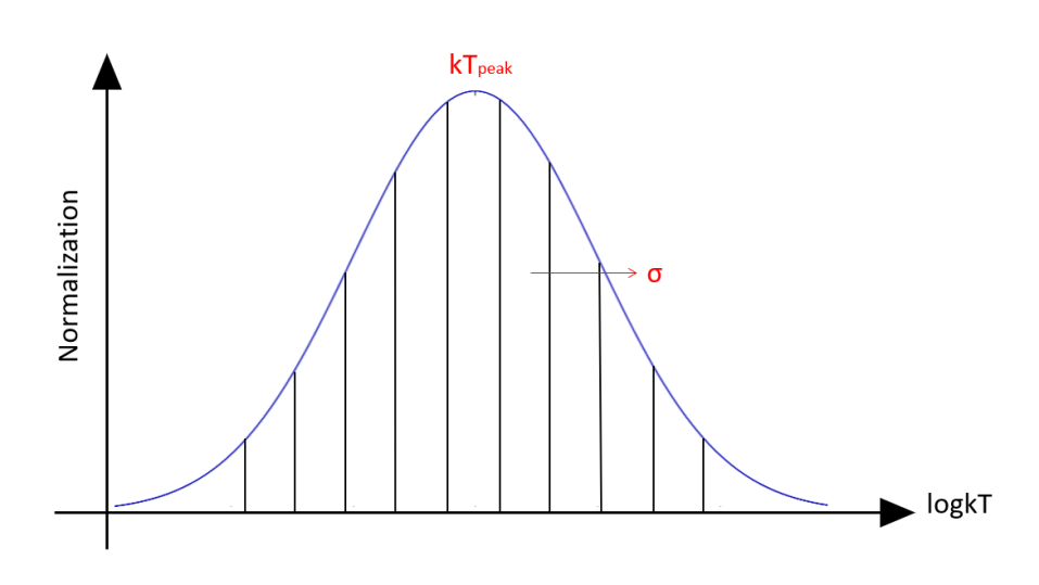
Figure 4: An illustration of the log-Gaussian temperature distribution model based on a fixed grid of single-temperature components. These parameters include the peak normalization (normpeak), the temperature of the peak (kTpeak), and the standard deviation of the distribution (sigma). Based on these parameters, the normalization is assigned following the Gaussian formula at each temperature (T) for the 10 APEC components.

3.2 Spectral Model

For the modeling process, we employed the APEC model (Smith et al., 2001). As a compromise between realistic modeling and handling moderate photon counts, we adopted a plasma with a log-Gaussian temperature distribution. Typically, a single-temperature plasma (with 2 free parameters: normalization and temperature) is assumed for relatively low-count spectra. The plasma is modeled using the Astrophysical Plasma Emission Code (APEC model), which has all metal abundances linked. However, high-quality M dwarf spectra show that the plasma temperature distribution is smooth and broad (Robrade & Schmitt, 2005). The temperature distributions resemble a log-Gaussian during quiescent phases, and also during flares, which typically exhibit a broader and hotter temperature distribution (Robrade & Schmitt, 2005). Therefore, we model the spectra with a plasma featuring a log-Gaussian temperature distribution. In practice, this is achieved by an ensemble of 10 APEC components on a logarithmic temperature grid, where the normalizations follow a bell curve as part of the modeling process in BXA. This is illustrated in Fig. 4. The free parameters are the peak temperature, peak normalization, and the width $\sigma$ of the log-Gaussian distribution. The list of priors is detailed in Table 5. These parameters control the normalization of each component, as depicted in Fig. 4.

Table 5: Priors set for the APEC model

Parameter	Prior	Range
p1.Abundanc	uniform	0.0 - 1.0
kTpeak	log-uniform	0.1 - 5.0
normpeak	log-uniform	$10^{-6}$ - 0.01
sigma	uniform	0.0 - 2.0

In addition, we have integrated background spectral models to offer additional information, considering smooth correlations between data bins and known instrument behaviors. This approach enhances information extraction from low-count data. We use the Chandra background model obtained through principal components analysis (PCA), as presented by Simmonds et al. (2018). Our analysis employs Poisson (C-Stat) statistics to jointly assess the background and source spectra.

3.3 Modeling of Atmospheric Escape

To assess the impact of X-ray radiation on the planet, we use the VPLanet model (Barnes et al., 2020). VPLanet conducts extensive simulations of planetary system evolution, spanning Gyr timescales, with a primary emphasis on studying habitable planets. Its modules encompass various aspects such as internal, atmospheric, rotational, orbital, stellar, and galactic processes. These modules can be interconnected to enable the concurrent simulation of the evolution of terrestrial planets, gaseous planets, and stars. The code’s validity is established through its capacity to replicate a range of observations and previously obtained results. In this work, we use some modules to estimate the influence of the observed XUV flux and predict water loss in the system. The simulation of atmospheric escape is conducted using the AtmEsc, STELLAR, and FLARE modules within the VPLanet framework. The AtmEsc module is designed to simulate the escape of planetary atmospheres and the release of surface volatiles based on energy-limited and diffusion-limited mechanisms. The VPLanet model has been developed based on previous research, indicating that for small planets, the escape rate correlates with the stellar XUV flux and inversely with the gravitational potential energy of the gas (Lopez et al., 2012; Lammer, 2013; Owen & Wu, 2017). Because of the limited knowledge of exoplanetary atmospheric structures, VPLanet employs the energy-limited approximation. All uncertainties concerning the escape process physics are encapsulated in the XUV escape efficiency ($\mathrm{\epsilon_{xuv}}$). The model assumes $\mathrm{\epsilon_{xuv}\sim}$ 0.1 as a reasonable median value, providing accurate escape flux predictions within a factor of a few. Thus, we note a caution here that the energy-limited formalism used in AtmEsc is an approximate description of atmospheric escape. It does not account for wavelength dependence in upper atmosphere heating, varying with composition and temperature structure, which is omitted from the model. The STELLAR module models key characteristics in low-mass stars ($\mathrm{M_{\star}\leq 1.4M_{{\odot}}}$), including radius, stellar radius of gyration ($\mathrm{r_{g}}$), effective temperature, bolometric luminosity, XUV luminosity, and rotation rate. This simulation employs bicubic interpolation over mass and time, with the Baraffe et al. (2015) models based on solar metallicity stars.

The FLARE modules (do Amaral et al., 2022) integrate the flare frequency distribution model proposed by Davenport et al. (2019) into the conventional STELLAR package. The integration of the two packages: STELLAR and FLARE reveals that flares contribute approximately 10% more XUV emission to M dwarfs compared with quiescent stellar levels. Such high XUV levels in the flaring star can result in the removal of up to an additional two terrestrial oceans (TO) of surface water on Earth-like planets, compared to the non-flaring star.

In our simulations, we place the three planets with observed mass, radius, and orbital radius (Winters et al., 2019, 2022; Lavie et al., 2022) around the star. The stellar model followed the Baraffe et al. (2015) model

The initial configuration includes 1.0 terrestrial ocean (TO) or an Earth’s worth of water. Once the hydrogen envelope is eliminated, XUV photons trigger the dissociation of water molecules, resulting in increased hydrogen escape and oxygen buildup in the atmosphere. The water escape is modeled based on Bolmont et al. (2017), taking into account the habitable zone limit from Kopparapu et al. (2013).

The examination of stellar evolution follows the trajectory of a stellar model described in Baraffe et al. (2015). This considers factors such as magnetic braking (Reiners et al., 2014) and the XUV evolution model. The simulation input parameters are based on the study of solar-type stars during their quiescent periods (Ribas et al., 2005).

The FLARE model in Fig. 8 is detailed in do Amaral et al. (2022), incorporating a relation between flare energy and frequency (Davenport et al., 2019), dependent on the star type and age. The FLARE module computes the average XUV for each simulation time-step, integrating from minimum to maximum flare energy. Generally, the inclusion of flares increases XUV luminosity by less than 10%. In our work, we assumed flare energies between $\mathrm{10^{30}}$ and $\mathrm{10^{33}}$ erg following Davenport et al. (2019). This study found that flare activity decreases as low-mass stars spin down and age. Additionally, the frequency distributions from observed stars in the Kepler field show no significant change in the power law slope with age. It is noteworthy that the Davenport et al. (2019) model over-predicts the superflare rate as it was constructed from younger and more active stars than the Sun, of which approximately 3% of the catalog samples (Davenport, 2016) are M-stars.

Finally, we explore atmospheric escape, also known as atmospheric evaporation—a phenomenon that can lead to planetary mass loss due to the influence of the host star. This occurs when high-energy radiation and charged particles from the host star ionize the gas molecules in the planet’s upper atmosphere, causing them to escape into space. The rate of atmospheric escape depends on several factors, including the planet’s mass, radius, composition, magnetic field, and distance from the host star. Notably, recent work by Ketzer & Poppenhaeger (2023) found that the natural scatter of stars in their spin-down evolution can have a significant impact on the accumulated mass loss of exoplanets. We determined the mass loss rate for three planets orbiting the A component—namely, LTT1445Ab and LTT1445Ac—using the following equation:

$$\dot{M}=\epsilon\times\frac{\pi R_{pl}F_{XUV}}{GM_{pl}/R_{pl}}$$ (1)

Here, $\dot{M}$ represents the mass loss rate, $\epsilon$ denotes the efficiency from the mass loss model (Lopez et al., 2012; Owen & Jackson, 2012; Foster et al., 2022), $R_{pl}$ stands for the planet radius, $M_{pl}$ for the planet mass, $G$ is the gravitational constant, and $F_{\rm XUV}$ combines the observed X-ray flux and the estimated EUV flux from the host star. The EUV luminosity of the star was derived from X-ray luminosity using Eq. 3 in Sanz-Forcada et al. (2011).

Secondly, the AtmEsc module (Barnes et al., 2020) is utilized to calculate Roche lobe overflow, thermal escape, and radiation-recombination-limited processes of an atmosphere. This incorporates water photolysis, hydrogen escape, oxygen escape, and oxygen build-up. The thermal escape is approximated with an energy-limited formula. The configuration parameters for VPLanet are reported in Table 6. Detailed information on the stars’ and planets’ parameters is provided in Tables 1 and 2, respectively (Winters et al., 2019, 2022; Lavie et al., 2022). The planetary characteristics in our simulation are modeled after Proxima Centauri b (Barnes et al., 2016). The simulation assumes a surface water abundance of 1.0 Terrestrial Ocean (TO), equivalent to the amount of water on Earth, employing the water escape efficiency detailed in Bolmont et al. (2017). The envelope mass of the planet is set at 0.001 $M_{\oplus}$. Our simulation encompasses flare energy within the observed flux range of $\mathrm{10^{29}}$ and $\mathrm{10^{33}}$ erg.

Table 6: Parameter of Star and Planets used for the simulation with VPLnet for LTT1445A

Parameter	Value
Envelope mass ($M_{{\oplus}}$)	0.001
Surface water (TO)	1.0
XUV water escape efficiency	Bolmont et al. (2017)
Thermosphere temperature (K)	400
Stellar mass ($M_{{\odot}}$)	0.257
Saturated XUV luminosity fraction	$\mathrm{10^{-3}}$
Initial Stellar Age (Gyr)	0.2
Flare Energy (erg)	$\mathrm{10^{33}}$ to $\mathrm{10^{36}}$

4 Results

Table 7: X-ray properties for LTT 1445A across observations

Date	Observatory	Activity	Duration	$f_{X}$	$\mathrm{logL_{X}}$	$kT_{peak}$	Ref.
			[ks]	[$\mathrm{10^{-13}\,ergcm^{-2}s^{-1}}$]		[keV]
2021-06-05	Chandra	Flare	6.66	$3.61\pm 0.27$	$27.31\pm 0.10$	$1.02\pm 0.10$	Brown 2022
2021-06-05	Chandra	Elevated	11.6	$0.66\pm 0.10$	$26.57\pm 0.07$	$0.59\pm 0.29$	Brown 2022
2021-06-05	Chandra	Quiescent	12.2	$0.066\pm 0.033$	$25.57^{+0.18}_{-0.30}$	$1.02\pm 0.10$	Brown 2022
2022-10-10	Chandra	Quiescent	12.0	$0.259^{+0.12}_{-0.08}$	$26.16\pm 0.24$	$0.80\pm 0.94$	This work
2022-10-12	Chandra	Quiescent	12.0	$0.19^{+0.15}_{-0.07}$	$26.0\pm 0.4$	$0.68\pm 0.87$	This work
2022-11-24	Chandra	Quiescent	30.0	$0.18^{+0.05}_{-0.05}$	$26.03\pm 0.13$	$0.94\pm 0.76$	This work

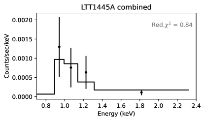
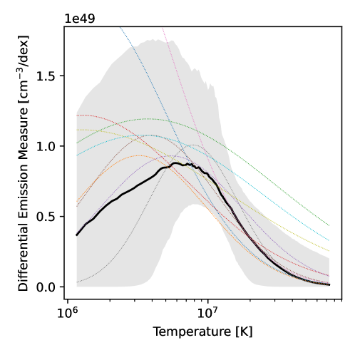
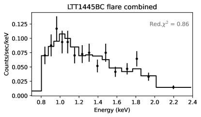
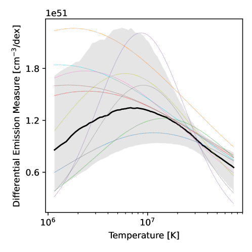
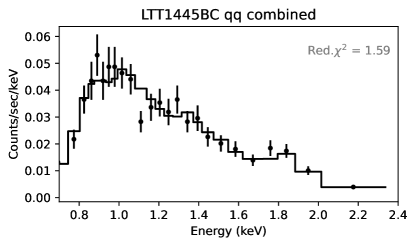
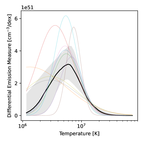
Figure 5: The left panels show the Chandra ACIS spectra of LTT 1445A combined (top panel) and LTT 1445BC combined Flare (middle) and Quasi-Quiescent (bottom). The corresponding right panels show the reconstructed continuous DEM distribution (approximated with a grid during the fit, see Fig.4). The black curve shows the median of the posterior DEM predictions, and the gray band contains 68% of the distribution. The colorful dotted lines are ten random posterior samples of possible DEM. The top right panel y-axis has a 100 times lower normalization than the lower right panels. The bottom right panel DEM has a narrow shape plummeting at $2\times 10^{7}\,\mathrm{K}$, while the middle right panel shows a broad distribution.

Table 8: X-ray properties for LTT 1445BC across observations

Date	Observatory	Activity	Duration	$f_{X}$	$\mathrm{logL_{X}}$	$kT_{peak}$	Ref.
			[ks]	[$\mathrm{10^{-13}\,ergcm^{-2}s^{-1}}$]		[keV]
2021-06-05	Chandra	Flare BC	5.2	$20.2\pm 0.90$	$28.06\pm 0.02$	$0.38\pm 0.1$*	Brown 2022
2021-06-05	Chandra	Nonflare BC	23.4	$7.3\pm 0.20$	$27.61\pm 0.01$	$0.76\pm 0.03$	Brown 2022
2022 all	Chandra	Flare BC	6.20	$14.9^{+0.93}_{-0.95}$**	$27.933\pm 0.027$	$0.81\pm 0.8$	This work
2022 all	Chandra	Nonflare BC	47.8	$7.63^{+0.34}_{-0.34}$**	$27.64\pm 0.019$	$0.43\pm 0.13$	This work
2022-10-12	Chandra	C - Full	12.0	$10.86^{+1.48}_{-1.09}$	$27.80\pm 0.05$	$0.33\pm 0.25$	This work
2022-11-24	Chandra	B - Full	30.0	$5.88^{+0.48}_{-0.59}$	$27.53\pm 0.04$	$0.82\pm 0.67$	This work

*The lower temperature ($kT_{1}$) from the two temperature fit
**Flux calculated for energy band 0.6-2.3 keV to match the eROSITA flux

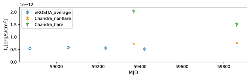
Figure 6: Variability of the BC components. The average flux taken from eROSITA eRASS1:4 (blue) every six months during the year 2020-2021. The Chandra observation from year 2021 was reported in Brown et al. (2022) and year 2022 from this work during the flare (green) and non-flare (orange) time.

In this section, we present the results derived from the analysis of X-ray spectra obtained from both Chandra and eROSITA observations. These observations provided X-ray properties, and the activity levels of the sources, as detailed in Section 4.1. Additionally, the eROSITA observation revealed X-ray variability spanning from eRASS1 to eRASS4, occurring two years before the Chandra observations. This variability is discussed in Section 4.2. We note that eROSITA is unable to distinguish the individual components in this system. We update the Rossby Number and bolometric correction ratio in Section 4.3. Lastly, the results from model predictions are presented in Section 4.4.

4.1 X-ray properties from spectral analysis

The spectral fits and parameter constraints from BXA and the plasma model APEC are presented in Fig. 5. For the spectral analysis of the A component, we combined all observations for a total duration of $50$ ks, resulting in the top panel of the figure.

Regarding the BC components, we specifically selected data from flaring periods, covering the time intervals of 1800-4000 s in the second observation and 14000-18000 s in the third observation in Fig.3. The corresponding spectrum from these flare periods is displayed in the middle panel of Figure 5. The remaining period from all three observations is categorized as ’quasi-quiescent’ (qq), and the respective spectrum is depicted in the bottom panel of Figure 5. Our spectral model incorporated the temperature distribution for the flare and quasi-quiescent periods, respectively. Our APEC model received a temperature distribution (kTdist) instead of a single-point temperature (kT1 or kT2). An advantage of using a temperature distribution is that it captures the behavior of the plasma temperature better than a single point, resulting in the distribution shape of the Differential Emission Measure (DEM) shown in the left panel of Fig.5.

In addition to the fitted spectral profile, we display the temperature distribution of each dataset from the 10-component grid model. The quiet period of A and the quasi-quiescent period of BC show an almost flat distribution at high temperatures, while the distribution of the BC flare consists of higher temperature components.

Despite the low counts, we allow the metal abundance as a free parameter in the APEC model. The obtained value for A’s abundances is 0.66$\pm$0.23 relative to the solar abundances. For BC during quasi-quiescent (qq), it is 0.141$\pm$0.045, and for BC during a flare, it is 0.49$\pm$0.21.

A comprehensive examination of the X-ray characteristics is provided in Table 7 for the A component and Table 8 for the BC component. The spectral analysis results demonstrate that each component exhibited similar X-ray luminosity levels both during A’s observation and throughout the BC observations. However, the BC component displayed X-ray luminosity levels approximately one order of magnitude higher than those observed for the quiescent A. Additionally, the BC component exhibited a peak in its temperature distribution at a higher value, as shown in the Differential Emission Measure panel, due to the stellar flare.

4.2 X-ray Variability

The BC components exhibit variability from both B and C at a similar level, as indicated in Table 8. Flare periods are observed for both B and C, as illustrated in the light curve in Fig. 3. Foster et al. (2022) reported a significant signal originating from the BC component from eRASS1.

However, due to the instrument’s spatial resolution, eROSITA cannot distinguish between the three components, and we report the eROSITA fluxes as totals for the entire system and assume the total is dominated by BC. Fig. 6 presents the flux from eRASS1 to eRASS4, along with the observed Chandra flux during flare and non-flare times for BC. We converted the 0.6-2.3 keV eROSITA count rates to fluxes with an APEC model, assuming a plasma temperature (kT) of 0.5 keV absorbed by $\log N_{\mathrm{H}}/\mathrm{cm}^{2}=19.5$ following Brown et al. (2022). If we adopt 1.0 keV instead, the flux becomes 6.6% lower. For Chandra, we obtain fluxes in the 0.6-2.3 keV range from the spectral fit shown in Fig. 5. A caveat here is that as of 2020, Chandra is most sensitive from 0.9-7 keV, while eROSITA has most sensitive energy range from 0.3-2.3 keV. This difference could lead to systematic discrepancies; refer to Figure 9 from Predehl et al. (2021) for more details. This could explain the offset between the lowest Chandra flux measurement to the eROSITA measurements.

4.3 X-ray Activity Levels

We evaluate the conformity of the observed X-ray activity with the standard behavior exhibited by M dwarfs, as illustrated in Fig. 7. The Rossby number ($R_{0}=P_{\text{rot}}/\tau$), representing the ratio of the rotation period ($P_{\text{rot}}$) to the convection turnover time ($\tau$), is calculated following Wright et al. (2011), as expressed in equation 5 from Wright et al. (2018). These investigations, primarily focused on F-G-K-M dwarfs, utilized ROSAT data for their analyses.

Rotation periods for A, B, and C, obtained from Winters et al. (2022), are 85, 6.7, and 1.4 days, respectively. The computed Rossby numbers for components A, B, and C are 1.3$\pm$1.2, 0.09$\pm$0.08, and 0.015$\pm$0.015, respectively, aligning well with the findings of Brown et al. (2022).

We have updated the X-ray bolometric luminosity ratios for the LTT1445 X-ray system. This involves calculating the luminosity ratio using the bolometric luminosity data from Winters et al. (2019) along with our observed average X-ray luminosities. Notably, the inclusion of the observed flare in B enhances the alignment of the data points with the anticipated relation outlined by Wright et al. (2018).

Figure 7: The updated Rossby Number and bolometric correction ratio from this work in blue and from Brown et al. (2022) in gray overlaid with the Wright et al. (2018) model.

During the Chandra observations in late 2022 (or Q4 2022), the A component was quiescent. At the same periods, BC switched the activity level. The updated activity relation is shown in Fig.7.

4.4 Model prediction

4.4.1 Stellar Evolution

We provide an overview of stellar evolution using the MDwarfLuminosity (do Amaral et al., 2022) module of the VPLanet package. This is illustrated in Fig. 8, where we explore the luminosity and structural changes that stars undergo from their formation until the culmination of the main sequence phase. Furthermore, this model interprets X-ray flares, quiescent fluxes, and their impact on the planets. For the flare energy, we follow Davenport et al. (2019), which suggests levels of $\mathrm{10^{33}}$ and $\mathrm{10^{36}}$  erg.

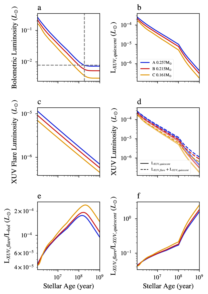
Figure 8: The stellar evolution track based on Baraffe et al. (2015) model of the three stars in the system. Panels (a) and (b) display the bolometric luminosity and the XUV quiescent luminosity. The observed bolometric luminosity was used to determine the A component to be 0.183 Gyr old (dashed lines). Panels (c) and (d) display the XUV luminosity from flares and the total XUV luminosity. The ratio of XUV luminosity from flares to bolometric luminosity is displayed in panel (e), and the ratio of XUV luminosity from flares to XUV quiescent luminosity is displayed in panel (f).

4.4.2 Atmospheric Escape

For terrestrial planets, VPLanet assumes atmospheres dominated by water vapor rather than H/He. This model follows a runaway greenhouse scenario, where atmospheric escape occurs only when the total incident flux on the planet surpasses the runaway greenhouse threshold (Kopparapu et al., 2013). In the context of water and oxygen loss, this occurs after the removal of the hydrogen envelope. Subsequently, XUV photons start the dissociation of water molecules, leading to increased hydrogen escape and, in certain scenarios, oxygen escape.

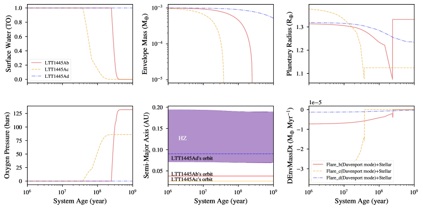
Figure 9: Atmospheric escape over time of the LTT 1445A. The panels show: (top left) the surface water starting from water abundance of 1.0 TO, (top cental) Envelop Mass loss of the three planets over time, (top right) the evolution of planetary radius, (bottom left) the amount of oxygen buildup in the atmosphere due to the XUV radiation, (bottom central) position of each planet from the habitable zone (HZ), (bottom right) envelope loss rate.

Figure 9 illustrates the outcomes of our simulations, indicating that planet c’s envelope was stripped away after 38 million years, while planet b’s envelope endured for 246 million years from the initial stellar age, set at 0.2 Gyr. Notably, planet d, initially thought to be within the habitable zone (HZ) according to Lavie et al. (2022), was reconsidered as being in the ’Too Hot’ zone (Fig.1) once the stellar age was taken into account. This HZ planet suggests the potential retention of surface water, while for the other planets, abiotic oxygen accumulation commenced following water loss. However, do Amaral et al. (2022) suggested that water content is more significantly influenced by stellar mass than planetary mass when water loss ceases upon reaching the HZ. Our assumptions include a primordial hydrogen envelope mass of 0.001 $M_{\oplus}$ and an initial water abundance of 1.0 Terrestrial Oceans (TO) for the system.

5 Discussion

The understanding of the intricate interplay between stars and their associated planets is pivotal for advancing future observations of rocky planets and refining the characterization of their atmospheres. In this section, various aspects of the star-planet interaction in the triple-star system LTT 1445 are explored, incorporating observational parameters to enhance and constrain theoretical models. This includes considerations of stellar evolution, the estimation of planetary mass loss, and atmospheric escape.

Determining the age of M dwarfs poses challenges (Stelzer et al., 2016; Magaudda et al., 2020), and the limited observation time provides only a narrow snapshot of the system. Despite these challenges, we integrated observed bolometric luminosity data Winters et al. (2019) with the Baraffe et al. (2015) model. It’s noteworthy that this model grid lacks XUV evolution, which is not well-constrained for M-dwarf stars. Our estimate suggests that the age of the LTT1445 system is approximately 0.18 Gyr (gray dashed line in Fig.8). This determination aligns with earlier estimates from both the observation reported in Brown et al. (2022) and the Hubble Space Telescope (HST) observation outlined in Pass et al. (2023). These works proposed that both BC components may represent a younger, faster-rotating star than the Sun.

Considering the differences in stellar mass within this system, theoretical considerations encompassing stellar evolution, interactions, three-body dynamics, and the initial population in stellar triples collectively contribute to variations in mass and stellar types. Simulations by Toonen et al. (2020) indicate that stellar interactions are common in triples. In contrast to binary populations, the proportion of systems capable of undergoing mass transfer is approximately 2-3 times greater in triple systems, resulting in varied mass within the system.

Insights into planet formation in complex stellar environments can be gleaned from the study of star formation and its effects on protoplanetary disks. Ronco et al. (2021) investigated a nearly 10 Myr old disk in the HD 98800 multiple system, which still retained significant amounts of gas. The study compared the evolution of gas disks in hierarchical triple-star systems and circumbinary systems. It revealed that in triple-star systems, gas surface density profiles evolve slowly, leading to higher midplane temperatures and aspect ratios compared to circumbinary systems. This could potentially facilitate planet formation in triple-star systems. Recent discoveries of protoplanetary disks in multiple-star systems also suggest that some of these disks can remain intact for much longer periods; for instance, Zagaria et al. (2021), observed that the motion of dust within circumstellar disks around one of the stars in a binary star system exhibits a higher drift rate compared to disks unaffected by an outer stellar companion.

In a conservative worst-case scenario for atmosphere loss, we utilize the X-ray flux of LTT1445A during the observed flare period in Brown et al. (2022). The determined mass loss rates are approximately $\mathrm{1.24\times 10^{9}g/s}$ for planet b, $\mathrm{3.22\times 10^{9}g/s}$ for planet c, and $\mathrm{2.93\times 10^{9}g/s}$ for planet d, considering a $R_{pl}$ value of 1.29 $R_{\oplus}$ for planet d.

In a triple-star system, planets can be exposed to flares not only from the host star but also from nearby stars. We assess the impact of BC on the planets orbiting A. The distance from A to BC is 34 AU, whereas the orbital distance of the planets is less than 0.1 AU. Consequently, due to the significant distance, the X-rays originating from A are 410² times more influential. Despite the largest observed flare from BC (luminosity of $10^{28.15}\,\mathrm{erg/s}$, Table 8), its impact on the planets is negligible compared to the irradiation from the most quiescent X-ray levels of A (luminosity of $10^{25.5}\,\mathrm{erg/s}$, Table 7).

The outcomes from VPLanet suggest that planet LTT 1445Ad could retain a water surface, whereas the other planet may facilitate abiotic oxygen accumulation up to pressures of 100-150 bars if the system initially possessed 1.0 TO. Consequently, a more accurate evaluation of this assumption requires precise measurements of water abundance to refine the model.

6 Summary

This study presents a comprehensive analysis of the long-term high-energy environment of LTT1445. The dataset encompasses three recent Chandra observations, coupled with continuous monitoring from eROSITA eRASS1 to eRASS4. The Chandra observations effectively differentiate coronal X-ray emissions from all three stars in the LTT 1445 system, including the exoplanet host star, LTT 1445A. Our primary findings are as follows:

• Concerning the star’s X-ray activity, LTT 1445C emerges as the primary source of X-ray emissions, with supplementary contributions from LTT 1445B. The study confirms that LTT 1445A, characterized by slow rotation, exhibits no significant flare activity in our observational dataset.

• The planets orbiting A receive irradiation from all M dwarfs. However, our findings suggest that the X-ray emission from the LTT 1445BC components does not pose a greater threat to the planets orbiting LTT 1445A than the emissions from A itself.

• If the system’s evolution begins with a water abundance of at least 1.0 TO, LTT 1445Ad could have an atmosphere.

• X-ray irradiation causes non-biotic oxygen build-up in the atmosphere of this nearby system.

Our simulations involved various parameters, including stellar mass, planetary mass, and initial water abundance, to delineate trajectories determining the current presence of water on the planetary surfaces. It is important to note that processes such as radiative cooling from substances such as $\mathrm{CO_{2}}$, tidal forces, planetary magnetic fields, or coronal mass ejections (CMEs) were not considered. However, in future studies, understanding whether these processes make a minor contribution or have the potential to significantly alter the overall picture would be crucial. Improving this assumption also necessitates more accurate measurements of water abundance to refine the model.

It is recommended that future panchromatic observations be conducted, utilizing space missions such as the James Webb Space Telescope and Athena, as well as ground-based facilities such as the Extremely Large Telescope. The presence of oxygen could be observed using novel instrumentation such as FIOS (Ben-Ami et al., 2018), where the ultra-high-resolution Fabry-Perot-based instrument will be employed to boost spectral resolution. This has recently been demonstrated in on-sky observations with telluric oxygen (Rukdee et al., 2023). For direct imaging of strongly illuminated planets, UNDERGROUND (Fowler et al., 2023) will observe the reflected light using a combination of a coronagraph and VIPA high-resolution spectrograph. These observations may validate the predictions presented here and potentially contribute to the discovery of an inhabited exoplanet.

Software

This work makes use of the following package: matplotlib (Hunter, 2007), scipy (Virtanen et al., 2020), astropy (Astropy Collaboration et al., 2013, 2018, 2022), BXA (Buchner et al., 2014), UltraNest (Buchner, 2021), CIAO/Sherpa (Fruscione et al., 2006), eSASS (Brunner et al., 2022) and VPLanet (Barnes et al., 2020) including package FLARE (do Amaral et al., 2022).