Post-inflationary Dark Matter production and Leptogenesis: Metric versus Palatini formalism

Abstract

We investigate production of non-thermal dark matter particle and heavy sterile neutrino from inflaton during the reheating era which is preceded by a slow-roll inflationary epoch with a quartic potential and non-minimal coupling ($\xi$) between the inflaton and the gravity. We compare our analysis between metric and Palatini formalism. For the latter with $\xi=0.5$ and number of $e$-folds $\sim 60$, $r$ can be as small as $\sim{\cal O}\left(10^{-3}\right)$ which may be validated at $1-\sigma$ CL of prospective future reaches of upcoming CMB observation such as CMB-S4 etc. We identify that permissible range of Yukawa coupling $y_{\chi}$ between inflaton and fermionic DM $\chi$, to be ${\cal O}\left(10^{-3.5}\right)\gtrsim y_{\chi}\gtrsim{\cal O}\left(10^{-20}\right)$ for metric formalism and ${\cal O}\left(10^{-4}\right)\gtrsim y_{\chi}\gtrsim{\cal O}\left(10^{-11}\right)$ for Palatini formalism which is consistent with current PLANCK data and also be within the reach of future CMB experiments. For the scenario of leptogenesis via the decay of sterile neutrino produced from inflaton decay, we also investigate the parameter space of heavy neutrino mass $m_{N_{1}}$ and Yukawa coupling $y_{N_{1}}$ of sterile neutrino with inflaton, which are consistent with current CMB data and successful generation of the observed baryon asymmetry of the universe via leptogenesis. In contrast to metric formalism, in the case of Palatini formalism for successful leptogenesis to occur we find that $y_{N_{1}}$ has a very narrow allowable range and is severely constrained from the consistency with CMB predictions.

I Introduction

The strongest evidences that upholds the standard model of cosmology comes from remarkable agreement between the theoretical prediction and observed data about Big Bang Nucleosynthesis (BBN), and the detection of CMB photons in the present universe. During the BBN era, which occurs when the temperature of the universe is between $\sim 1\,\text{MeV}$ and $\sim 10\,\text{keV}$, light elements e.g. deuterium, helium-3, helium-4, and lithium-7 are formed Bambi and Dolgov (2015). The production mechanism for these elements during BBN is based on well established theory of standard model (SM) of particle physics. Consequently, the abundance of those light elements put stringent constraints on BSM physics.

Conversely, numerical analysis of data obtained from CMB also places constraints on cosmological parameters such as present-day energy density of baryons and dark matter (DM), among others. Almost all elementary particles in the SM of particle physics that exist in our universe have corresponding antiparticles with the same mass and lifetime but with opposite charges. All those SM particles were relativistic in the early universe, when the temperature was higher than the mass of the top-quark. We assume their chemical potential was negligible at that time so they existed likely in local thermal equilibrium with the SM photons which suggests that the numbers of particles and antiparticles were initially equal. Therefore, the matter-antimatter asymmetry observed in our present observable universe remains unexplainable. The ratio of the number density of baryons to photons in the present universe obtained from CMB is $\eta_{B}\sim 6.14\times 10^{-10}$ Aghanim et al. (2020); Zyla et al. (2020); Fields et al. (2020). This result is consistent with BBN analysis and observed small fraction of antiproton (${\cal O}\quantity(10^{-4})$) and anti-helium-4 (${\cal O}\quantity(10^{-7})$) from cosmic rays Bambi and Dolgov (2015), and the ratio of antibaryon to baryon obtained from the two colliding clusters of galaxies in Bullet Cluster Steigman (2008). Moreover, if there is a nearby antimatter domain, it must not be located inside the cosmological horizon. Consequently, a universe characterized by matter-antimatter symmetry is empirically ruled out Cohen et al. (1998). The predominance of matter over antimatter in the early universe can be generated through a dynamic physical process if that violates (i) baryon number B, (ii) C- and CP-invariance, and (iii) thermal equilibrium Sakharov (1967). These conditions are known as Sakharov principles. Although, numerous baryogenesis mechanisms have been proposed, including decay of heavy particles Sakharov (1967), via evaporation of primordial black holes Hawking (1974); Zeldovich (1976), the most extensively studied ones being electroweak baryogenesis Kuzmin et al. (1985); Shaposhnikov (1986, 1987) and baryogenesis through leptogenesis Fukugita and Yanagida (1986). Among them the latter involves the decay of heavy right-handed neutrinos, introduced as an extension to the SM to achieve light neutrino masses via the Type-I seesaw mechanism Minkowski (1977); Gell-Mann et al. (1979); Yanagida (1979); Mohapatra and Senjanovic (1980); Mohapatra (2004), and also addresses the puzzle of tiny neutrino mass generation which is evident from several neutrino oscillation experiments.

Furthermore, CMB data, along with by several other independent cosmological observations, reveals that cold dark matter (CDM) contributes to $\sim 26\%$ of total mass-energy density of the universe Aghanim et al. (2020); Workman et al. (2022). This contribution is almost five times that of visible matter. The particle nature of dark matter remains a an enigma to date, as no direct detection of DM experiment found any evidence including the most popular candidate for particle DM - Weakly Interacting Massive Particles (WIMPs). Iis is assumed that WIMP particles were in thermal equilibrium in the early universe, and then they decoupled at a later time. Several unsuccessful attempts to detect such particles through the scattering of atomic nuclei or electrons, or by detecting the products of their decay from cosmic rays Bergstrom et al. (2013); Cuoco et al. (2018), or in particle detectors at CERN ATL (2022); Pedro (2023); Giagu (2019), brings forth the alternative assumptions that DM particles are so much feebly interacting that they could never reach in thermal equilibrium in the early universe. They could be produced from the decay of massive particles in the early universe, and unlike thermal DM, their relic density depends on the specific production channels.

Observation of the temperature of CMB photons over the full sky reveals that temperature anisotropy is even less than $10^{-5}$ in contrast to the expectation of the last scattering surface being $\sim 10^{5}$ causally disconnected patches Kamionkowski and Kosowsky (1999). This implies that the largest length scale that enters the causal Horizon today must have existed well inside the earliest epoch. The simplest way to envision such a scenario is by proposing that there was an early epoch during which the energy density of a slowly rolling scalar field, $\phi$, referred to as inflaton, along the slope of its potential dominated the universe. This minimal modification to the standard model of cosmology effectively accounts for the generation of primordial perturbation and flatness of our universe. Although further validation of the inflationary paradigm is still on the cards, this is widely accepted as the new standard model of cosmology within the scientific community. Despite its stupendous success in overcoming the limitations of Big Bang cosmology and providing the required amount of seeds of matter perturbations, the minimal models of chaotic inflation involving potential $\propto\phi^{p}$, where $p$ is an integer number, appear to be disfavored by the latest data released by Planck mission Aghanim et al. (2020) and data from Bicep+Keck Array Ade et al. (2021) regarding unobserved B-mode of primordial tensor perturbations from inflaton. However, as revealed in subsequent studies Boubekeur et al. (2015); Bezrukov (2008); Kallosh and Linde (2013), the scenario can be reinstated, bringing these models back to the limelight, by considering that the inflaton is non-minimally coupled to gravity. Such a coupling can be generated from quantum correction Hertzberg (2010), and provides a plateau-like region for the inflation to occur.

An interesting possibility arises when the inflaton is non-minimally coupled to gravity, the predictions of slow-roll inflation, such as the scalar spectral index ($n_{s}$) and tensor-to-scalar ratio ($r$), may vary between the metric and Palatini formalisms (see Capozziello:2010ih,Kallosh:2013tua,Jarv:2017azx,Racioppi:2017spw,Refs. Ref. Capozziello et al. (2011); Kallosh et al. (2014); Järv et al. (2018); Racioppi (2017)). For small or near-zero values of non-minimal coupling yield nearly identical predictions in both formalisms, but larger values lead to differences. In the metric formalism, for an inflaton potential $V(\phi)\propto\phi^{p}$, $n_{s}$ and $r$ remain independent of non-minimal coupling at the leading order. Conversely, in the Palatini formalism, the predicted values of $r$ vary inversely with non-minimal coupling Cheong et al. (2022).

In metric formalism, space-time metric ($g_{\alpha\beta}$) and its first derivative are the independent variables, whereas in Palatini formalism, space-time metric and metric connection (or, affine connection which is denoted by $\Gamma^{\lambda}_{\alpha\beta}$) are independent variables Bostan (2023); Racioppi (2020). In differential geometry, metric connection measures the intrinsic curvature of the manifold. In metric formalism, it is assumed that $\Gamma^{\lambda}_{\alpha\beta}=\Gamma^{\lambda}_{\beta\alpha}$ and $\nabla_{\lambda}g_{\alpha\beta}=0$, and as a result affine connection is replaced by Levi-Civita connection, $\bar{\Gamma}_{\alpha\beta}^{\lambda}$, which is defined as Bauer and Demir (2008) $\bar{\Gamma}_{\alpha\beta}^{\lambda}=\frac{1}{2}{g^{JF}}^{\lambda\zeta}\left[\partial_{\alpha}\left({g^{JF}}_{\beta\zeta}\right)+\partial_{\beta}\left({g^{JF}}_{\alpha\zeta}\right)-\partial_{\zeta}\left({g^{JF}}_{\alpha\beta}\right)\right].$  In the theory of general relativity, the preference for the Levi-Civita connection arises not only because the torsion part of the connection disappears, but also due to the Equivalence Principle and the importance of aligning affine geodesics and metric geodesics to uphold causality Borunda et al. (2008). Consequently, in metric formalism, Riemann curvature tensor depends on the second derivative of the space-time metric. Conversely, in Palatini formalism, Riemann curvature tensor depends on the first derivative of the space-time metric Bauer and Demir (2008), and Ricci tensor depends on connection but independent of the metric tensor Borunda et al. (2008). Moreover, in the Palatini formulation, increasing $\xi$ values reduces the value of $r$ significantly ($r\sim{{\cal N}_{\text{CMB}}}^{-2}$ in metric formalism, and $r\sim\left(\xi\,{\cal N}_{\text{CMB}}\right)^{-2}$ in Palatini formalism, with ${\cal N}_{\text{CMB}}$ denoting the number of $e$-folds of inflation Shaposhnikov et al. (2020)). This provides a potential pathway for rescuing inflationary models which have been ruled out by CMB observations for predicting large values of $r$ within the metric formalism Racioppi (2017); Artymowski and Racioppi (2017); Kannike et al. (2016); Barrie et al. (2016). The end of inflation is followed by reheating era that acts as a bridge to transform the inflaton dominated cold universe into our familiar universe dominated by relativistic standard model particles Allahverdi et al. (2010).

In this article we plan to investigate post-inflationary dark matter production and leptogenesis parallelly within these two formalisms. Inflaton can also generate stable but light particles contributing to dark radiation Ghoshal et al. (2023a). In this study, our focus is on a scenario that involves both the inflaton and a gauge singlet BSM field which if stable is the CDM candiate or can be the unstable right-handed neutrino which decays to SM particles leading to baryogenesis via leptogenesis. For a list of models incorporating inflation and DM, see Ghoshal:2022jeo,Refs. Ref. Ghoshal et al. (2022a) and references therein. In our work, we assume that BSM vectorlike fermionic particles are produced during the reheating era through the decay of inflaton. These particles are assumed stable, non-relativistic, but feebly interacting with the SM relativistic plasma, and contributes to the total CDM density of the universe. We also consider another possibility when a sterile neutrino is produced from the decay of inflaton. Their decay is out-of-equilibrium, C and CP violating process (with 1-loop effects) and violates lepton number thereby satisfying Sakharov’s conditions Sakharov (1967). Then, baryon-lepton number violating sphaleron processes coverts lepton asymmetry to baryon asymmetry, see. Asaka:1999yd,Co:2022bgh,Senoguz:2004ky,Asaka:1999jb,Barrie:2021mwi,Refs. Ref. Asaka et al. (1999); Co et al. (2022); Senoguz and Shafi (2004); Asaka et al. (2000); Barrie et al. (2022)

This paper is organized as follows: in Sec. II, we discuss the Lagrangian density of inflation non-minimally coupled to gravity, as well as the interaction Lagrangian density during reheating. In Sec. III, we study the benchmark for slow roll inflationary scenario with a quartic potential of inflaton. In Sec. IV, we present the stability analysis. In Sec. V, we focus on reheating and production of non-thermal BSM particles as CDM. In Sec. VI we explore leptogenesis from the decay of sterile neutrino.

In this work, we use $\hbar=c=k_{B}=1$ and the value of reduced Planck constant $M_{P}=2.4\times 10^{18}\,\text{GeV}$. In addition, we assume that the space-time metric is diagonal with signature $(+,-,-,-)$.

II Lagrangian Density

In this article, our focus is on the reheating era following a slow roll inflation, where we consider the non-minimal coupling between the inflaton $\varphi$ and the curvature scalar ${\cal R}$, and the production of a fermionic BSM particle alongside the SM Higgs particle $h$ during reheating. Then, the action for inflation in Jordan frame is given by Bostan and Şenoğuz (2019); Markkanen et al. (2018)

$${\cal S}^{JF}\supset\int\text{d}^{4}x\sqrt{-g^{JF}}\left(\frac{1}{2}M_{P}^{2}\,\Omega^{2}(\varphi)\,\mathscr{R}^{JF}+\frac{1}{2}\left(\partial\varphi\right)^{2}-V^{JF}(\varphi)\right)\,.$$ (1)

We use $JF$ in superscript to refer that the corresponding quantity is defined in Jordan frame. Therefore, $g^{JF}$, $\mathscr{R}^{JF}$, and $V^{JF}(\varphi)$ are the determinant of the space-time metric, Ricci scalar and potential of the inflaton in Jordan frame, respectively. Additionally, we consider the form of $\Omega^{2}(\varphi)\equiv\Omega^{2}\neq 0$ as

$$\Omega^{2}(\varphi)=1+\xi\frac{\varphi^{2}}{M_{P}^{2}}\,,$$ (2)

where both $\Omega^{2}$ and $\xi$ are dimensionless. In Einstein frame, the gravity sector and $\varphi$ are not coupled. The metric in Einstein frame, denoted by $g^{E}_{\mu\nu}$, can be obtained as

$$g^{E}_{\mu\nu}=\Omega^{2}\,g^{JF}_{\mu\nu}\,.$$ (3)

In this article, Greek indices in both subscript and superscript range from $0$ to $3$. Additionally, we employ Einstein’s summation convention for repeated indices. In Einstein frame, the potential for inflaton is

$$V^{E}(\varphi)=\frac{V^{JF}\left(\varphi\right)}{\Omega^{4}\left(\varphi\right)}\,.$$ (4)

Furthermore, to make the kinetic term of inflaton canonical in Einstein frame, we need to redefine the inflaton as $\phi$. The relation between $\phi$ and $\varphi$ is given by Ghoshal et al. (2023b)

$$\derivative{\phi}{\varphi}=\sqrt{\Pi(\varphi)}\,,$$ (5)

where Shaposhnikov et al. (2020); Racioppi (2020); Park and Yamaguchi (2008)

$$\Pi(\varphi)=\frac{1}{\Omega^{2}}+\kappa\frac{3}{2}\left(\frac{M_{P}}{\Omega^{2}}\partialderivative{\quantity(\Omega^{2})}{\phi}\right)^{2}\,,\qquad\kappa=\begin{cases}1\,\,\text{(metric formalism)}\,,\\ 0\,\,\text{(Palatini formalism)}\,.\end{cases}$$ (6)

In metric formalism space-time metric, and other fields (for example, $\varphi$ in Eq. 1) are the independent dynamical variables, while in Palatini formalism $\Gamma_{\alpha\beta}^{\lambda}$ is also independent dynamical variable in addition to $\varphi$ and space-time metric Bauer and Demir (2008). Moreover, in Palatini formalism Riemann tensor remains invariant under the transformation of Eq. 3 Bauer and Demir (2008). For the form of $\Omega^{2}$ mentioned in Eq. 2, we have

$$\sqrt{\frac{1+\left(1+6\xi\right)\xi\varphi^{2}/M_{P}^{2}}{\left(1+\xi\varphi^{2}/M_{P}^{2}\right)^{2}}}\,\, \text{(metric formalism)}\,,$$ (7)

$$\frac{1}{\sqrt{1+\xi\varphi^{2}/M_{P}^{2}}}\,\,\,\; \text{(Palatini formalism)}\,.$$ (8)

Now, integrating Eq. 7, we get Rasanen and Wahlman (2017); Garcia-Bellido et al. (2009)

$$\sqrt{\xi}\frac{\phi}{M_{P}}=\sqrt{6\kappa\xi+1}\sinh^{-1}\left(u\sqrt{6\kappa\xi+1}\right)-\sqrt{6\kappa\xi}\tanh^{-1}\left(\frac{\sqrt{6\kappa\xi}u}{\sqrt{u^{2}(6\kappa\xi+1)+1}}\right)\,,$$ (9)

where $u=\sqrt{\xi}\frac{\varphi}{M_{P}}$. In metric formalism, under small field limit (i.e. $u\ll 1$ such that $\quantity(1+u^{2})\approx 1$ and $\quantity(1+u^{2}+6\xi u^{2})\approx 1$) Bezrukov and Shaposhnikov (2009), and under $\sqrt{\xi}u\gg 1$ we obtain Bezrukov and Shaposhnikov (2008)

$$\varphi\simeq\begin{cases}\phi\,,\qquad&(\text{for }\sqrt{\xi}\varphi\ll M_{P})\\ \frac{M_{P}}{\sqrt{\xi}}\exp(\frac{1}{\sqrt{6}}\frac{\phi}{M_{P}})\,\qquad&(\text{for }\xi\varphi\gg M_{P})\end{cases}$$ (10)

However, in Palatini formalism, we can get exact relation between $\varphi$ and $\phi$ from Eq. 8 as follows

$$\varphi=\frac{M_{P}}{\sqrt{\xi}}\sinh(\sqrt{\xi}\frac{\phi}{M_{P}})\,.$$ (11)

The relation between $\varphi$ and $\phi$ in Eq. 10 is approximated, whereas the relation in Eq. 11 is exact.

Moving forward, we assume that the interaction of inflaton with fermionic field $\chi$, which is singlet under SM gauge transformations, and with SM Higgs field $H$ during post-inflationary reheating era are defined in Einstein frame, and the interaction Lagrangian can be written as Ghoshal et al. (2022a, b, 2023b, 2023c)

$$\mathcal{L}_{{\rm rh}}=-y_{\chi}\phi\bar{\chi}\chi-\lambda_{12}\phi H^{\dagger}H-\lambda_{22}\phi^{2}H^{\dagger}H+\text{h.c.}+\cdots\,,$$ (12)

Among the three couplings $y_{\chi},\lambda_{12},\lambda_{22}$, only $\lambda_{12}$ has mass dimension. Moreover, in Eq. 12, ellipses denote scattering of $\chi$ by SM particles or inflaton. However, we assume those interactions are not strong enough to keep $\chi$-particles in local-thermal equilibrium with the SM relativistic plasma of the universe. From Bernal:2021qrl,Refs. Ref. Bernal and Xu (2021), and also from our previous studies Ghoshal et al. (2023b, d, 2022a), it has been found that these scattering channels are not effective in producing enough $\chi$ particles such that total CDM density is satisfied, unless $\chi$ particles are highly massive (with a mass $m_{\chi}\sim{\cal O}\quantity(10^{10}\,\text{GeV})$ or larger). As a result, our current focus in this article is solely on the production of $\chi$ particles through the decay of the inflaton. For the sake of completeness, the Lagrangian density of $\chi$ and $H$ are given below

$${\cal L}_{\chi}^{E} =i\bar{\chi}\gamma^{\mu}{\partial_{\mu}}\chi-m_{\chi}\bar{\chi}\chi\,,$$ (13)

$${\cal L}_{H}^{E} =\left(\partial H\right)^{2}+m_{H}^{2}H^{\dagger}H-\lambda_{H}\left(H^{\dagger}H\right)^{2}\,,$$ (14)

where $i=\sqrt{-1}$, $\gamma^{\mu}$ are the four gamma matrices and $\bar{\chi}=\chi^{\dagger}\gamma^{0}$, and $\lambda_{H}>0$. In Sec. V of this article, we investigate whether $\chi$, vector-like fermionic stable particles produced through the decay of inflaton, contribute $100\%$ of the total CDM density of the present universe. In contrast, in Sec. VI, we explore the possibility of $\chi$ as a sterile yet unstable neutrino, generating lepton asymmetry immediately after its production.

III Quartic potential

In this article, we consider potential of inflaton in Jordan frame as Gialamas et al. (2023); Markkanen et al. (2018); Takahashi and Tenkanen (2019); Racioppi and Vasar (2022)

$$V^{JF}(\varphi)=\Lambda\,\varphi^{4}\,,$$ (15)

where $\Lambda$ is dimensionless. If we consider quantum loop correction arising due to the interaction of inflation with a fermionic and a scalar field, the potential for inflaton in Jordan frame is best described by Coleman-Weinberg potential (for example, see Ref. Kannike et al. (2017); Racioppi et al. (2022); Okada and Raut (2017)). However, this form of potential for slow roll inflation is in tension with the best-fit $n_{s}-r$ contour obtained from Planck2018+Bicep3 combined data Racioppi (2017), unless the renormalization scale is super Planckian Ghoshal et al. (2023d). Since our focus in this work is to examine possible (in)consistencies, if any, in the metric and Palatini formalism, we restrict ourselves to considering only the simple quartic form of the inflationary potential.

The potential of inflation in Einstein frame can be written as

$$V^{E}(\varphi)=\frac{\Lambda\,\varphi^{4}}{\Omega^{4}(\varphi)}\,.$$ (16)

In metric formalism and for $\xi\varphi\gg M_{P}$, the potential for inflaton mentioned in Eq. 16 is given by Takahashi and Tenkanen (2019)

$$V^{E}_{(m)}(\phi)\simeq\frac{\Lambda\,M_{P}^{4}}{\xi^{2}}\left(e^{-\sqrt{\frac{2}{3}}\frac{\phi}{M_{P}}}+1\right)^{2}\,,$$ (17)

and under small field limit Takahashi and Tenkanen (2019)

$$V^{E}_{(m)}(\phi)\approx\frac{2}{3}\frac{\Lambda}{\xi^{2}}M_{P}^{2}\,\phi^{2}\,.$$ (18)

In Palatini formalism, the potential of inflaton in Einstein frame Gialamas et al. (2023); Takahashi and Tenkanen (2019)

$$V^{E}_{(P)}(\phi)=M_{P}^{4}\frac{\Lambda}{\xi^{2}}\quantity(\tanh(\sqrt{\xi}\frac{\phi}{M_{P}}))^{4}$$ (19)

Under small field approximation (assuming $\sqrt{\xi}\phi/M_{P}<\pi/2$) Takahashi and Tenkanen (2019)

$$V_{(P)}^{E}(\phi)\approx\Lambda\phi^{4}$$ (20)

From Eqs. 18 and 20 we see that during reheating when inflaton oscillates about the minimum, potential is quadratic in metric formalism and quartic in Palatini formalism Takahashi and Tenkanen (2019).

Under slow roll approximation, the observables of the inflationary epoch, namely scalar spectral index ($n_{s}$), tensor to scalar ratio ($r$), and amplitude of comoving curvature power spectrum ($A_{s}$) are defined in Einstein frame as follows Baumann (2011)

$$n_{s}(\phi_{*})\simeq 1-6\,\epsilon_{V}^{E}(\phi_{*})+2\,\eta_{V}^{E}(\phi_{*})\,,\quad r(\varphi_{*})\approx 16\,\epsilon_{V}^{E}(\phi_{*})\,, V^{E}(\phi_{*})\simeq\frac{3}{2}\pi^{2}\,r(\phi_{*})\,A_{s}\,M_{P}^{4}\,.$$ (21)

Here $\phi_{*}$ is the value of inflaton corresponding to the pivot scale of CMB observations, whereas $\epsilon_{V}^{E}(\phi)$, and $\eta_{V}^{E}(\phi)$ are the potential slow roll parameters defined as Lyth and Liddle (2009); Okada and Raut (2017) $\epsilon_{V}^{E}(\phi)=\quantity({M_{P}^{2}}/{2})\,\quantity({\differential\ln[V^{E}]}/{\differential\phi})^{2}$ and $\eta_{V}^{E}(\phi)=\quantity(M_{P}^{2}/V^{E})\quantity({\differential^{2}V^{E}}/{\differential\phi^{2}})$. During slow roll inflationary epoch $\epsilon_{V}^{E},\eta_{V}^{E}\ll 1$. Current bounds on $n_{s}$, $r$, and $A_{s}$ are mentioned in Table 1. The duration of the inflationary epoch is expressed in terms of the number of e-folds (${\cal N}_{\text{CMB}}$) which is defined as Baumann (2011)

$${\cal N}_{\text{CMB}}=M_{P}^{-1}\int^{\phi_{*}}_{\phi_{\rm end}}\quantity(2\,\epsilon_{V}^{E})^{-1/2}\,\differential\phi\,,$$ (22)

where $\phi_{\rm end}$ is the value of the inflaton at which the slow roll phase ends, i.e., when the kinetic energy of the inflaton becomes $\sim V^{E}(\phi)$. In other words, it happens when any of $\epsilon_{V}^{E}$ or $\eta_{V}^{E}$ becomes $\sim 1$ Ghoshal et al. (2022a). In this article, we consider $50\leq{\cal N}_{\text{CMB}}\leq 60$.

Table 1: Constraints on $n_{s},r$ and $A_{s}$ (T and E for temperature and E-mode polarization of CMB).

$\ln(10^{10}A_{s})$	$3.044\pm 0.014$	$68\%$, TT,TE,EE+lowE+lensing+BAO	Aghanim et al. (2020); Workman et al. (2022)
$n_{s}$	$0.9647\pm 0.0043$	$68\%$, TT,TE,EE+lowE+lensing+BAO	Aghanim et al. (2020)
$r$	$0.014^{+0.010}_{-0.011}\,\text{and}$	$95\%\,,\text{BK18, {Bicep}3, {Keck Array}\leavevmode\nobreak\ 2020,}$	Aghanim et al. (2020); Ade et al. (2022, 2021)
	$<0.036$	and WMAP and Planck CMB polarization	(see also Campeti and Komatsu (2022))

Using the relation between $\phi$ and $\varphi$ from Eq. 11 (for Palatini) and exact expression from Eq. 9 (for metric), while varying $\xi$, we obtain benchmark values for slow roll inflation for both the metric and Palatini formalism. These benchmark values satisfy the bounds presented in Table 1 and are obtained for ${\cal N}_{\text{CMB}}\sim 50$ and $60$. These benchmarks are listed in Tables 3 and 2 ($\varphi_{*}$ and $\varphi_{\rm end}$ in Jordan frame correspond to the value of $\phi_{*}$ and $\phi_{\rm end}$ in Einstein frame). Here, we are mainly interested in the regime where $\xi\gg 1$, as in this case, the predictions between the metric and Palatini formalisms exhibit significant differences Cheong et al. (2022). This will help us make the kind of comparison we intend to do between the two formalisms. In either of the metric or Palatini formalism,  Tables 2 and 3 indicate that for a constant value of $\xi$, the value of $\varphi_{\rm end}$ (or $\phi_{\rm end}$) remains fixed.

Table 2: Benchmark values for slow roll inflation in metric formalism.

Benchmark	$\xi$	$\varphi_{\rm end}/M_{P}$	$\varphi_{*}/M_{P}$	${\cal N}_{\text{CMB}}$	$n_{s}$	$r\times 10^{3}$	$\Lambda$
(m)BM1	$0.5$	$1.3287$	$11.2724$	$60$	$0.9677$	$3.9483$	$3.1644\times 10^{-11}$
(m)BM2			$10.3349$	$50$	$0.9614$	$5.5837$	$4.5015\times 10^{-11}$
(m)BM3	$10$	$0.3372$	$2.8886$	$60$	$0.9678$	$3.0132$	$9.5886\times 10^{-9}$
(m)BM4			$2.6488$	$50$	$0.9616$	$4.2620$	$1.3624\times 10^{-8}$
(m)BM5	$10^{2}$	$0.1074$	$0.9203$	$60$	$0.9678$	$2.9688$	$9.4441\times 10^{-7}$
(m)BM6			$0.8439$	$50$	$0.9616$	$4.1993$	$1.3417\times 10^{-6}$
(m)BM7	$10^{4}$	$0.0107$	$0.0921$	$60$	$0.9678$	$2.9639$	$9.4283\times 10^{-3}$
(m)BM8			$0.0845$	$50$	$0.9616$	$4.1924$	$1.3395\times 10^{-2}$

Table 3: Benchmark values for slow roll inflation in Palatini formalism.

Benchmark	$\xi$	$\varphi_{\rm end}/M_{P}$	$\varphi_{*}/M_{P}$	${\cal N}_{\text{CMB}}$	$n_{s}$	$r\times 10^{3}$	$\Lambda$
(P)BM1	$0.5$	$1.7672$	$21.9801$	$60$	$0.9668$	$1.0923$	$8.5554\times 10^{-12}$
(P)BM2			$20.0779$	$50$	$0.9602$	$1.5675$	$1.2298\times 10^{-11}$
(P)BM3	$10$	$0.9197$	$21.9282$	$60$	$0.9667$	$5.5349\times 10^{-2}$	$1.7206\times 10^{-10}$
(P)BM4			$20.0211$	$50$	$0.9601$	$7.9643\times 10^{-2}$	$2.4760\times 10^{-10}$
(P)BM5	$100$	$0.5271$	$21.9152$	$60$	$0.9667$	$5.5490\times 10^{-3}$	$1.7243\times 10^{-9}$
(P)BM6			$20.0069$	$50$	$0.9600$	$7.9887\times 10^{-3}$	$2.4825\times 10^{-9}$
(P)BM7	$10^{4}$	$0.1680$	$21.9095$	$60$	$0.9667$	$5.5549\times 10^{-5}$	$1.7261\times 10^{-7}$
(P)BM8			$20.0007$	$50$	$0.9600$	$7.9989\times 10^{-5}$	$2.4855\times 10^{-7}$

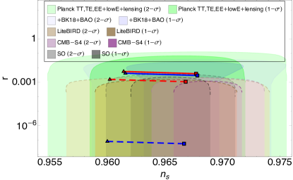
Figure 1: $(n_{s}-r)$ predictions for $\xi=0.5$ and $\xi=10^{4}$ in both metric and Palatini formalism and for $50\lesssim{\cal N}_{\text{CMB}}\lesssim 60$ along with bounds on $(n_{s}-r)$ plane from CMB observations (Planck2018, Bicep3, Keck Array) and prospective future reach from upcoming CMB experiments (LiteBIRD,CMB-S4,SO Hazumi et al. (2020); Abazajian et al. (2016); Ade et al. (2019)). The solid straight lines correspond to $(n_{s},r)$ predictions in metric formalism - red color line for $\xi=0.5$ and blue colored line for $\xi=10^{4}$. The dashed straight lines correspond to $(n_{s},r)$ predictions in Palatini formalism - red colored line for $\xi=0.5$ and blue colored line for $\xi=10^{4}$. Along the lines, ${\cal N}_{\text{CMB}}$ is varied from $50$ to $60$ from left to right.

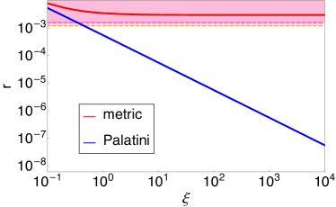
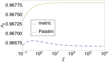
Figure 2: Left-pannel: Variation of predicted value of $r$ against $\xi$ for ${\cal N}_{\text{CMB}}=60$ for metric and Palatini formalisms. The pink-colored and Yellowish orange-colored regions represent the values of $r$ which can be validated at $1-\sigma$ CL by the upcoming CMB experiments LiteBIRD, and CMB-S4, respectively. Right-pannel: Variation of the predicted value of $n_{s}$ against $\xi$ for ${\cal N}_{\text{CMB}}=60$ for metric and Palatini formalisms.

Fig. 1 displays the $n_{s}-r$ predictions for slow roll inflation corresponding to the potential of the inflaton mentioned in Eq. 16, in both metric and Palatini formalisms. The solid straight lines are for predictions in metric formalism: red colored line for $\xi=0.5$, while blue colored line for $\xi=10^{4}$. The dashed straight lines are for predictions in Palatini formalism: red colored line for $\xi=0.5$, while blue colored line for $\xi=10^{4}$. Along these lines, ${\cal N}_{\text{CMB}}$ varies between $50$ to $60$, marked with a triangular symbol at ${\cal N}_{\text{CMB}}\simeq 50$ and a square symbol at ${\cal N}_{\text{CMB}}\simeq 60$. Fig. 1 also shows bounds on the $n_{s}-r$ plane from observed CMB data from Planck2018 and Planck2018+Bicep3+Keck Array2015 combined analysis, along with future prospective reaches for upcoming CMB experiments (with dashed curved lines as perimeter) e.g. CMB-S4, LiteBIRD, Simons Observatory (SO), shown in the background. This figure shows that while the predicted values of $(n_{s},r)$ in both the metric and Palatini formalisms, for both ${\cal N}_{\text{CMB}}=50$ and ${\cal N}_{\text{CMB}}=60$, fall within the $1-\sigma$ best-fit contour of Planck2018 data, those predicted values for ${\cal N}_{\text{CMB}}$ around $50$ (${\cal N}_{\text{CMB}}\gtrsim 50$) are excluded at the $1-\sigma$ CL by the combined analysis of Planck+Bicep+Keck Array data. Furthermore, LiteBIRD,CMB-S4, and SO can verify all $(n_{s},r)$ values, particularly those predicted within the metric formalism. For example, predicted values of $(n_{s},r)$ in metric formalism for ${\cal N}_{\text{CMB}}\sim 60$ can be tested by upcoming SO at $1-\sigma$ CL. For the predicted values of $(n_{s},r)$ in Palatini formalism around ${\cal N}_{\text{CMB}}\sim 50$ for $\xi=0.5$ can be tested in the future by LiteBIRD at $1-\sigma$ CL or by SO at $2-\sigma$ CL, and around ${\cal N}_{\text{CMB}}\sim 60$ for $\xi=0.5$ can be verified by upcoming CMB-S4 at $1-\sigma$ CL. The predicted values of $(n_{s},r)$ in Palatini formalism around ${\cal N}_{\text{CMB}}\sim 50$ for $\xi=10^{4}$ can be validated in the future by forthcoming SO at $1-\sigma$ CL. From Tables 2 and 3 and Fig. 1, we see that predicted values $r$, at a fixed value of $\xi$, exhibit a decrease as value of ${\cal N}_{\text{CMB}}$ increases. This is due to $\ln\left(r\right)\propto-\ln\left({\cal N}_{\text{CMB}}\right)$ observed in both formalisms Cheong et al. (2022). Furthermore, Fig. 2 depicts variation of $n_{s}$ and $r$ with $\xi$ for ${\cal N}_{\text{CMB}}\sim 60$. Comparatively, $r$ exhibits more significant variation with $\xi$ than $n_{s}$, specifically, in Palatini formalism. This can be explained as follows: when $\xi\gg 1$, at leading order approximation $r\sim\xi^{0}$ in metric formalism, while $r\sim\xi^{-1}$ in Palatini formalism Cheong et al. (2022). Furthermore, in the left panel, the areas shaded in pink and yellowish-orange depict the valuse of $r$ which can be validated at $1-\sigma$ CL by the forthcoming CMB experiments LiteBIRD and CMB-S4, respectively. Therefore, this future CMB observation can refute or validate at $1-\sigma$ CL the analysis of slow roll inflation in metric formalism for the plain quartic potential of inflaton and with nonminimal coupling with Ricci scalar.

IV Stability

In this section, we explore the permissible upper limit of $y_{\chi}$ and $\lambda_{12}$ such that the radiative loop correction arising due to coupling of inflaton with $\chi$ and $H$ does not distort the flatness of the potential $V^{E}_{(m)}$ or $V^{E}_{(P)}$. Actually, We focus on reheating via $\lambda_{12}$, assuming a very small permissible value for $\lambda_{22}$. Here, we use exact expression of $V^{E}_{(m)}$ rather than relying on an approximate expression, such as the expression given in Eq. 17. In this section, we use $V^{E}_{\rm tree}$ to denote $V^{E}_{(m)}$ or $V^{E}_{(P)}$ and call them as tree level potential. The Coleman–Weinberg (CW) correction to the inflaton potential is Coleman and Weinberg (1973)

$$V_{{\rm 1-loop}}=\sum_{j}\frac{n_{j}}{64\pi^{2}}(-1)^{2s_{j}}\widetilde{m}_{j}^{4}\left[\ln\left(\frac{\widetilde{m}_{j}^{2}}{\mu^{2}}\right)-c_{j}\right]\,.$$ (23)

Here, inflaton dependent mass for $j\equiv\chi$ and for $j=H$ are $\widetilde{m}_{\chi}^{2}(\phi)=\left(m_{\chi}+y_{\chi}\phi\right)^{2}$ and $\widetilde{m}_{H}^{2}(\phi)=m_{H}^{2}+\lambda_{12}\phi$, respectively. Furthermore, $c_{j}=\frac{3}{2}$; $n_{H,\chi}=4$; $s_{H}=0$, $s_{\chi}=1/2$; and, we consider two values of the renormalization scale: $\mu=\phi_{*}$ and $\mu=\phi_{\rm end}$. Now, the first and second derivatives of the Coleman–Weinberg term of Eq. 23 for $\chi$ and $H$ with respect to $\phi$ are Drees and Xu (2021)

$$V_{{\rm 1-loop}}^{\prime}=\sum\limits_{j}\frac{n_{j}}{32\pi^{2}}(-1)^{2s_{j}}\widetilde{m}_{j}^{2}\,\left(\widetilde{m}_{j}^{2}\right)^{\prime}\left[\ln\left(\frac{\widetilde{m}_{j}^{2}}{\mu^{2}}\right)-1\right]\,,$$ (24)

$$V_{{\rm 1-loop}}^{\prime\prime}=\sum\limits_{j}\frac{n_{j}}{32\pi^{2}}(-1)^{2s_{j}}\left\{\left[\left(\left(\widetilde{m}_{j}^{2}\right)^{\prime}\right)^{2}+\widetilde{m}_{j}^{2}\left(\widetilde{m}_{j}^{2}\right)^{\prime\prime}\right]\ln\left(\frac{\widetilde{m}_{j}^{2}}{\mu^{2}}\right)-\widetilde{m}_{j}^{2}\left(\widetilde{m}_{j}^{2}\right)^{\prime\prime}\right\}\,.$$ (25)

The upper permissible values of $y_{\chi}$ and $\lambda_{12}$ can be obtained if both of the following conditions are simultaneously satisfied (with $m_{\chi}\approx m_{H}\approx 0$)

$$\left|V_{{{\rm 1-loop}},j}^{\prime}(\phi=\mu)\right|<V_{\rm tree}^{\prime}(\phi=\mu)\,, \left|V_{{{\rm 1-loop}},j}^{\prime\prime}(\phi=\mu)\right|<V_{\rm tree}^{\prime\prime}(\phi=\mu)\,.$$ (26)

From this point forward, we work with two benchmark values corresponding to $\xi=10$ and $\xi=10^{4}$ to demonstrate the dependence on the results on the coupling parameter. We select these benchmark values with $\xi\gg 1$ to distinctly differentiate between the metric and Palatini formalisms, as discussed earlier. Furthermore, we select benchmarks corresponding to ${\cal N}_{\text{CMB}}=60$, as predicted $(ns,r)$ values fall within the $1-\sigma$ contour of Planck+Bicep combined analysis on the $n_{s}-r$ plane. The upper limit of $y_{\chi}$ and $\lambda_{12}$ from stability analysis are mentioned in Table 4 for metric formalism (Benchmark: (m)BM3 and (m)BM7) and in Table 5 for Palatini formalism (Benchmark: (P)BM3 and (P)BM7).

Table 4: Allowed upper limit of $y_{\chi}$ and $\lambda_{12}$ for the benchmark values (m)BM3 and (m)BM7 from Table 2.

Benchmark	stability for $y_{\chi}$		stability for $\lambda_{12}$
	about $\mu=\phi_{*}$	about $\mu=\phi_{\rm end}$	about $\mu=\phi_{*}$	about $\mu=\phi_{\rm end}$
(m)BM3	$y_{\chi}<4.0723\times 10^{-4}$	$y_{\chi}<1.4026\times 10^{-3}$	$\lambda_{12}/M_{P}<1.3157\times 10^{-6}$	$\lambda_{12}/M_{P}<1.7633\times 10^{-5}$
(m)BM7	$y_{\chi}<4.8013\times 10^{-4}$	$y_{\chi}<2.0114\times 10^{-3}$	$\lambda_{12}/M_{P}<1.8197\times 10^{-6}$	$\lambda_{12}/M_{P}<3.8608\times 10^{-5}$

Table 5: Allowed upper limit of $y_{\chi}$ and $\lambda_{12}$ for the benchmark values (P)BM3 and (P)BM7  from Table 3.

Benchmark	stability for $y_{\chi}$		stability for $\lambda_{12}$
	about $\mu=\phi_{*}$	about $\mu=\phi_{\rm end}$	about $\mu=\phi_{*}$	about $\mu=\phi_{\rm end}$
(P)BM3	$y_{\chi}<2.8987\times 10^{-4}$	$y_{\chi}<1.2861\times 10^{-3}$	$\lambda_{12}/M_{P}<1.0050\times 10^{-7}$	$\lambda_{12}/M_{P}<7.8871\times 10^{-6}$
(P)BM7	$y_{\chi}<2.0864\times 10^{-4}$	$y_{\chi}<2.4894\times 10^{-3}$	$\lambda_{12}/M_{P}<1.3483\times 10^{-8}$	$\lambda_{12}/M_{P}<1.7057\times 10^{-6}$

From Tables 4 and 5 we infer the following upper limits of $\lambda_{12}$ and $y_{\chi}$ (i.e. ${\lambda_{12}}_{,{\rm max}}$, and ${y_{\chi}}_{,{\rm max}}$) that respect the stability criteria: for (m)BM3, $y_{\chi}<4.0723\times 10^{-4}$ and $\lambda_{12}/M_{P}<1.3157\times 10^{-6}$; for (m)BM7, $y_{\chi}<4.8013\times 10^{-4}$ and $\lambda_{12}/M_{P}<1.8197\times 10^{-6}$; for (P)BM3, $y_{\chi}<2.8987\times 10^{-4}$ and $\lambda_{12}/M_{P}<1.0050\times 10^{-7}$; and for (P)BM7, $y_{\chi}<2.0864\times 10^{-4}$ and $\lambda_{12}/M_{P}<1.3483\times 10^{-8}$.

V Reheating and production of $\chi$ from inflaton decay

The inflationary epoch is succeeded by the reheating era, during which the adiabatic production of SM and possibly BSM particles from the oscillating inflaton takes place. Consequently, the universe transitions from a cold to a hot radiation-dominated state as the inflaton decays. With the formation of radiation (relativistic SM particles), the temperature of the universe rises to its maximum ($T_{max}$) and subsequently decreases due to Hubble expansion. Actually, in the early stages of reheating, the total reaction rate ($\Gamma_{\phi}$) of the inflaton is lower than the Hubble parameter (${\cal H}$), with the latter being the primary factor causing a decrease in the energy density of the oscillating inflaton. As the universe continues to expand, at reheat temperature ($T_{\rm rh}$), ${\cal H}$ becomes comparable to $\Gamma_{\phi}$, resulting in $\rho_{\phi}=\rho_{\text{rad}}$, indicating equality in energy density between the oscillating inflaton ($\rho_{\phi}$) and radiation ($\rho_{\text{rad}}$). Following this, the remaining energy density of inflaton quickly converts to SM and BSM particles, marking the beginning of radiation radiation-dominated universe. In this work, we investigate perturbative reheating, and we assume that the SM particles generated during this epoch rapidly achieve thermal equilibrium soon after their formation.

The equation of state parameter of the oscillating inflaton, $w_{\phi}$, can be defined as $w_{\phi}=P_{\phi}/\rho_{\phi}$ where, $P_{\phi}$ denotes the pressure of the oscillating inflaton. As $\phi$ oscillates rapidly, $w_{\phi}$ varies between $-1$ and $+1$, corresponding to the oscillation of inflaton from its maximum value to its minimum (in our case, minimum is at $\phi_{\rm min}=0$). Therefore, it is customary to define averaged equation of state $w_{{\rm re}}=\expectationvalue{w_{\phi}}$ such that $w_{{\rm re}}$ is constant or varies very slowly. If the potential of the inflaton about the minimum during reheating $V^{E}(\phi)\propto\phi^{k}$, then it can be shown that Lin (2023a, b); Ellis et al. (2015)

$$w_{\rm re}\simeq\frac{k-2}{k+2}\,.$$ (27)

Therefore, from Eqs. 18 and 20, we can infer that

$$w_{\rm re}\simeq\begin{cases}0\,\quad&\text{(in metric formalism)}\,,\\ \frac{1}{3}\,\quad&\text{(in Palatini formalism)}\,.\end{cases}$$ (28)

Hence, in metric formalism, inflaton behaves as non-relativistic fluid, whereas in Palatini formalism inflaton behaves as relativistic fluid. The primary reason behind this is that in Palatini formalism, $V_{(P)}^{E}(\phi)\sim\phi^{4}$, making $\phi$ massless and causing its evolution as radiation i.e. $\rho_{\phi}\sim\boldsymbol{a}^{-4}$ Garcia et al. (2020). From now on, we will use “(in metric formalism)” and “(in Palatini formalism)” to provide a side-by-side comparison of the results obtained using the condition that the potential of inflaton around the minimum is quadratic in metric formalism and quartic potential in Palatini formalism. Note that this difference in results might not be a generic feature for every model of inflation. In certain cases, the potential around the minimum could be quadratic in both the metric and Palatini formalisms. However, that we can find significant difference between the two formalisms for a class of inflationary models is a salient point of the present analysis, that needs to be explored further as we go along.

Following the discussion of Appendix B, we define $T_{\rm rh}$ in both metric and Palatini formalisms as

$$T_{\rm rh}\simeq \sqrt{\frac{2}{\pi}}\left(\frac{10}{g_{\star}}\right)^{1/4}\sqrt{M_{P}}\sqrt{\Gamma_{\phi}}\,,$$ (29)

where $\Gamma_{\phi}$ is the total decay width of inflaton. This particular choice in defining $T_{\rm rh}$ ensures that $\rho_{\phi}(T_{\rm rh})=\rho_{\text{rad}}(T_{\rm rh})$. However, $T_{max}$ depends on whether the potential of inflaton is quadratic or quartic during reheating. $T_{max}/T_{\rm rh}$ for the quadratic and quartic potential of inflaton during reheating is derived in Appendix B. Since, the potential about the minimum of the inflaton is quadratic in metric formalism, and quartic in Palatini formalism for our considered inflationary scenario, we obtain from Eq. 90 and Eq. 91 Bernal et al. (2019); Giudice et al. (2001); Garcia et al. (2020)

$$\left(\frac{3}{8}\right)^{2/5}\,\left(\frac{{\cal H}_{I}}{{\cal H}(T_{\rm rh})}\right)^{1/4}\,\quad \text{(in metric formalism)}\,,$$ (30)

$$\frac{3^{1/4}}{2}\,\left(\frac{{\cal H}_{I}}{{\cal H}(T_{\rm rh})}\right)^{1/4}\,\quad \text{(in Palatini formalism)}\,.$$ (31)

Here, we assume the effective number of relativistic degrees of freedom $g_{\star}\approx 106.75$. Furthermore, ${\cal H}_{I}$ denotes the value of Hubble parameter at the end of inflation (i.e. when $\rho_{\rm rad}=0$ Giudice et al. (2001)), which is given by

$${\cal H}_{I}\simeq\sqrt{\frac{V^{E}\quantity(\phi_{\rm end})}{3M_{P}^{2}}}\,.$$ (32)

Furthermore, ${\cal H}(T_{\rm rh})$ is the value of Hubble parameter when $T=T_{\rm rh}$, i.e.

$${\cal H}(T_{\rm rh})\simeq\frac{\pi}{3M_{P}}\sqrt{\frac{g_{\star}}{10}}\,T_{\rm rh}^{2}\,.$$ (33)

Considering Eq. 12, $\Gamma_{\phi}$ depends on decay width of inflaton to SM Higgs particle ($h$), denoted as $\Gamma_{\phi\to{hh}}$, and BSM particle ($\chi$), denoted as $\Gamma_{\phi\to\chi\chi}$. These are given by

$$\Gamma_{\phi}=\Gamma_{\phi\to{hh}}+\Gamma_{\phi\to\chi\chi}\approx\Gamma_{\phi\to{hh}}\,,$$ (34)

$$\Gamma_{\phi\to{hh}}\simeq\frac{\lambda_{12}^{2}}{8\pi\,m_{\phi}}\,,\qquad\Gamma_{\phi\to\chi\chi}\simeq\frac{y_{\chi}^{2}\,m_{\phi}}{8\pi}\,.$$ (35)

The reason for using the approximate sign in Eq. 34 is to prevent the universe from being dominated by DM immediately after reheating era. In Eq. 35 $m_{\phi}$ is the effective mass of inflaton in Einstein frame which can be obtained for both metric and Palatini formalisms as

$$m_{\phi}^{2}=\left.\frac{\text{d}^{2}V^{E}}{\text{d}\phi^{2}}\right|_{\phi=\phi_{\rm min}}\,.$$ (36)

The value of $m_{\phi}=0$ in both formalisms because the potential from Eq. 4 has a minimum at $\phi=0$. However, we can always add a bare mass term ${{{m_{b}}}}^{2}\,\phi^{2}$ to the potential. To ensure that the slow roll inflationary scenario discussed in Sec. III, holds good even after the inclusion of this bare mass term, an upper limit is imposed on the bare mass and it has been discussed in Appendix C. By using Eqs. 18, 101 and 100 we prefer to choose the value of bare mass as follows

$${{m_{b}}}_{(m),\xi}=\frac{1}{\upzeta}\,\sqrt{\frac{2}{3}\frac{\Lambda}{\xi^{2}}M_{P}^{2}}\,,$$ (37)

$${{m_{b}}}_{{(P)},\xi}\simeq\frac{1}{\upzeta}\,\sqrt{\Lambda}\left(\frac{\sqrt{3}\,M_{P}\,\lambda_{12}^{2}}{8\pi\,{\Lambda}}\right)^{1/3}=\frac{1}{\upzeta}\,\left(\frac{3\pi^{2}}{40}\right)^{1/4}\,\quantity(g_{\star}\,\Lambda)^{1/4}\,T_{\rm rh}\,,$$ (38)

where we have used Eq. 29. Additionally, $\upzeta$ is dimensionless numerical factor, and we prefer to choose $\upzeta=10$ and $\upzeta=100$ in this work.

Now, Fig. 3 displays the variation of $T_{max}/T_{\rm rh}$ against $T_{\rm rh}$: left panel provides a comparative view of variation of $T_{max}/T_{\rm rh}$ in metric (for benchmark value (m)BM3) and Palatini formalisms (for benchmark value (P)BM3), for same values of $\upzeta=10$, ${\cal N}_{\text{CMB}}=60$ (and also for $\xi=10$). The gray-colored vertical stripe on the left represents the lower bound on $T_{\rm rh}\gtrsim 4\times 10^{-3}\,\text{GeV}$ Giudice et al. (2001). The colored vertical stripes on the right side represent those values of $T_{\rm rh}$ are not allowed. The maximum allowed values of $T_{\rm rh}$ correspond to the maximum allowed values of $\lambda_{12}$ as mentioned in Tables 4 and 5 . The bound for (m)BM3 scenario is represented by the deep cyan stripe, whereas for (P)BM3 scenario is shown by the deep blue (lighter tinted) region. From the left panel of Fig. 3 we see that $T_{max}/T_{\rm rh}$ is greater in metric formalism (solid line) than in Palatini (dashed line) ($T_{max}/T_{\rm rh}=5.0665\times 10^{8}$ for (m)BM3, while $T_{max}/T_{\rm rh}=3.3999\times 10^{8}$ for (P)BM3, at $T_{\rm rh}=4\times 10^{-3}\,\text{GeV}$) for the same values of $\xi$ and ${\cal N}_{\text{CMB}}$. Right panel of Fig. 3 depicts $T_{max}/T_{\rm rh}$ vs. $T_{\rm rh}$ for two benchmark values in Palatini formalism - (P)BM3 and (P)BM7. It shows $T_{max}/T_{\rm rh}$ decreases with higher values of $\xi$ ($T_{max}/T_{\rm rh}=1.4736\times 10^{8}$ for (P)BM7, at $T_{\rm rh}=4\times 10^{-3}\,\text{GeV}$) which happens because potential becomes more flat for larger values of $\xi$. The same conclusion is also true in metric formalism, but the difference is not so much noticeable in comparison to Palatini formalism (e.g. $T_{max}/T_{\rm rh}=5.0665\times 10^{8}$ for (m)BM7at $T_{\rm rh}=4\times 10^{-3}\,\text{GeV}$). In the case of (P)BM3 scenario, the bound correspond to the maximum allowable value of $T_{\rm rh}$ for is denoted by the deep blue but lightly shaded vertical stripe, whereas, for (P)BM7 scenario, it is shown by the deep blue (darker shaded) region. To derive the maximum allowable value on $T_{\rm rh}$, we have considered $\upzeta=10$ for both panels. For $\upzeta>10$, the maximum allowable value of $T_{\rm rh}$ would increase further.

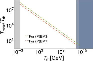
Figure 3: Variation of $T_{max}/T_{\rm rh}$ against $T_{\rm rh}$. Left panel: shows $T_{max}/T_{\rm rh}$ is less in Palatini formalism for same values of $\xi$ and ${\cal N}_{\text{CMB}}$. Right panel: shows $T_{max}/T_{\rm rh}$ decreases with increasing $\xi$ in Palatini formalism for same values of ${\cal N}_{\text{CMB}}$. Solid line for metric formalism (actually for benchmark (m)BM3), whereas dashed lines for Palatini formalism. The gray-colored stripe on the left denotes that $T_{\rm rh}\nless 4\,\text{MeV}$ are not allowed, and colored vertical stripes on the right indicates those values of $T_{\rm rh}$ are not allowed from the stability analysis from Tables 4 and 5.

V.1 Production of DM through decay

In this section, we investigate the case when the $\chi$-particles are produced from the decay of inflaton during the reheating era. We further assume that these $\chi$-particles, being both stable and non-thermal, act as viable DM candidates. Our aim is to explore the conditions under which these $\chi$-particles could potentially contribute to the entirety of the present-day CDM density in the universe. If $n_{\chi}$ and $N_{\chi}$ denotes the number density and comoving number density of DM particles, then the evolution equation of comoving number density of $\chi$ is

$$\frac{\differential N_{\chi}}{\differential t}=\boldsymbol{a}^{3}\,\gamma\,,$$ (39)

where $\gamma$ is the rate of production of $n_{\chi}$ and for $(\phi\to\bar{\chi}\chi)$

$$\gamma=2\,\text{Br}\,\Gamma_{\phi}\,\frac{\rho_{\phi}}{m_{\phi}}\,.$$ (40)

Here, ’Br’ denotes branching fraction for the production of $\chi$ from the decay process, and using Eqs. 34 and 35, it can be expressed as Ghoshal et al. (2023d, b)

$$\text{Br}=\frac{\Gamma_{\phi\to\bar{\chi}\chi}}{\Gamma_{\phi}}\approx m_{\phi}^{2}\left(\frac{y_{\chi}}{\lambda_{12}}\right)^{2}\,.$$ (41)

Following Appendix B, for $T_{max}>T>T_{\rm rh}$, ${\cal H}$ and $\rho_{\phi}$ can be defined as Bernal and Xu (2021)

$${\cal H}\simeq\frac{\pi}{3}\sqrt{\frac{g_{\star}}{10}}\frac{T^{4}}{M_{P}\,T_{\rm rh}^{2}}\,,\qquad \rho_{\phi}\simeq\frac{\pi^{2}g_{\star}}{30}\frac{T^{8}}{T_{\rm rh}^{4}}\,.$$ (42)

Using Eqs. 40, 41, 42 and 92 in Eq. 39, we can obtain DM yield, $Y_{\chi}$ which is defined as the ratio of number density of $\chi$ to entropy density, as

$$\frac{3}{\pi}\frac{g_{\star}}{g_{\star,s}}\sqrt{\frac{10}{g_{\star}}}\frac{M_{P}\,\Gamma_{\phi}}{m_{\phi}\,T_{\rm rh}}\text{Br}\,\quad\text{(in metric formalism)}\,,$$ (43)

$$\frac{9}{2\pi}\frac{g_{\star}}{g_{\star,s}}\sqrt{\frac{10}{g_{\star}}}\frac{M_{P}\,\Gamma_{\phi}}{m_{\phi}\,T_{\rm rh}}\text{Br}\,\quad\text{(in Palatini formalism)}\,.$$ (44)

Present day CDM yield is given by

$$Y_{{\rm CDM},0}=\frac{4.3.\times 10^{-10}}{m_{\chi}/\,\text{GeV}}\,.$$ (45)

The condition $Y_{\chi}\sim Y_{{\rm CDM},0}$ leads to

$$6.4907\times 10^{25}\,y_{\chi}^{2}\,m_{\chi}\,\quad\text{(in metric formalism)}\,,$$ (46)

$$9.7360\times 10^{25}\,y_{\chi}^{2}\,m_{\chi}\,\quad\text{(in Palatini formalism)}\,.$$ (47)

If DM particles are produced from the decay of inflaton during reheating era in our considered inflationary scenario, and account for $100\%$ of the total CDM density of the present universe, then it must satisfy Eqs. 46 and 47. These equations are represented as dotted lines for various fixed values of $y_{\chi}$ on $(T_{\rm rh},m_{\chi})$ plane, as shown in Fig. 4. Top-left panel of this figure for metric formalism (for (m)BM3 with $\upzeta=10$), top-right panel for Palatini formalism (for (P)BM3 with $\upzeta=10$ and $\upzeta=100$), and bottom panel for Palatini formalism but for (P)BM3 and (P)BM7 with $\upzeta=10$. The bounds on $(T_{\rm rh},m_{\chi})$ plane are mentioned below.

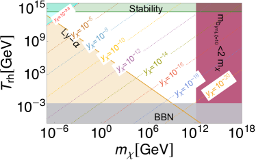
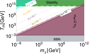
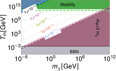
Figure 4: The allowed region (unshaded area) on $(T_{\rm rh},m_{\chi})$ plane and viable range for the Yukawa-like coupling $y_{\chi}$ to produce the entire CDM of the present universe: top-left panel: is for benchmark (m)BM3, top-right panel: is for benchmark (P)BM3 with bounds delimited by solid lines for $\upzeta=10$ and dashed lines for $\upzeta=100$, bottom panel: is for benchmark (P)BM3 and (P)BM7 with bounds delimited by solid lines for $\xi=10$ and dashed lines for $\xi=10^{4}$, both for $\upzeta=10$.

• The maximum permissible value $T_{\rm rh}$: This bound corresponds to the maximum permissible value of $T_{\rm rh}$ which in turn correspond to the maximum allowed value of $\lambda_{12}=\lambda_{12,{\rm max}}$ from Tables 4 and 5. This bound can be obtained from Eqs. 29, 37 and 38, and it is as follows:

  $$\sqrt{\frac{2}{\pi}}\left(\frac{10}{g_{\star}}\right)^{1/4}\sqrt{M_{P}}\left(\frac{\lambda_{12,{\rm max}}^{2}}{8\pi\,{{m_{b}}}_{(m),\xi}}\right)^{1/2}\,\quad \text{(for metric)}\,,$$ (48)

  $$\sqrt{\frac{\upzeta}{2}}\left(\frac{1}{3\,\pi^{10}\,\Lambda}\right)^{1/12}\left(\frac{10}{g_{\star}}\right)^{1/4}{M_{P}}^{1/3}{\lambda_{12,{\rm max}}}^{2/3}\,\quad \text{(for Palatini)}\,.$$ (49)

  This is displayed as horizontal forest-green or pastel-green shaded horizontal stripe placed at the upper side of the plots.

• The maximum value of $y_{\chi}$: This bound corresponds to the maximum permissible value of $y_{\chi}={y_{\chi}}_{,{\rm max}}$ obtained from Tables 5 and 4. This bound varies in metric and Palatini formalism as outlined below (from Eqs. 46 and 47):

  $$6.49\times 10^{25}\,{y_{\chi}}_{\rm max}^{2}\,m_{\chi}\,,\quad\text{(in metric formalism)}$$ (50)

  $$9.74\times 10^{25}\,{y_{\chi}}_{\rm max}^{2}\,m_{\chi}\,.\quad\text{(in Palatini formalism)}$$ (51)

  This is displayed as cyan colored (or deep blue colored on plot at the bottom plane) wedge-shaped region at the left-corner of the plots.

• The maximum possible value of $m_{\chi}$ in decay process: which is $m_{\chi}\lesssim{{m_{b}}}_{(m),\xi}/2$ (in metric formalism), and $m_{\chi}\lesssim{{m_{b}}}_{(P),\xi}/2$ (in Palatini formalism). In metric formalism, the region for $m_{\chi}>{{m_{b}}}_{(m),\xi}/2$ is indicated by a vertical copper-rose stripe on the right-side of the plot. However, in the Palatini case, due to the dependence of ${{m_{b}}}_{(P),\xi}$ on $T_{\rm rh}$, the representation for the region $m_{\chi}>{{m_{b}}}_{(P),\xi}/2$ changes to a wedge-shaped copper-rose region instead of a vertical stripe.

• Lyman-$\alpha$ bound: This constraint guarantees that $\chi$-particles do not contribute to warm dark matter, but rather to CDM. Since the $\chi$-particles are feebly interacting, their velocity can only decrease due to redshift. Based on this the lower bound on $m_{\chi}$, as derived in Bernal:2021qrl,Refs. Ref. Bernal and Xu (2021) (see also discussion in Ghoshal:2022jeo,Refs. Ref. Ghoshal et al. (2022a)), is

  $${m_{\chi}}\gtrsim 2\times 10^{-6}\frac{m_{\phi}}{T_{\rm rh}}\,\,\text{GeV}\,.$$ (52)

  In top-left panel (for the case of metric formalism) it is denoted by the peach-colored wedge-shaped region at the left bottom of the plot. However, in Palatini formalism, this bound can be obtained from Eq. 38 as

  $$m_{\chi}\gtrsim \frac{2\times 10^{-6}}{\upzeta}\,\left(\frac{3\pi^{2}}{40}\right)^{1/4}\,\quantity(g_{\star}\,\Lambda)^{1/4}\,\,\text{GeV}\,$$ (53)

  $$\gtrsim \begin{cases}2.1596\times 10^{-9}\,\text{GeV}\,\quad&(\text{for (P)BM3 with}\,\upzeta=10,\Lambda=1.7206\times 10^{-10})\,,\\ 2.1596\times 10^{-10}\,\text{GeV}\,\quad&(\text{for (P)BM3 with}\,\upzeta=100,\Lambda=1.7206\times 10^{-10})\,,\\ 1.2154\times 10^{-8}\,\text{GeV}\,\quad&(\text{for (P)BM7 with}\,\upzeta=10,\Lambda=1.7261\times 10^{-7})\,.\end{cases}$$ (54)

• BBN : $T_{rh}\gtrsim 4\,\text{MeV}$. This is presented as horizontal slate-gray stripe at the bottom of the plots.

The unshaded region in the plot at top-left panel of Fig. 4 represents the permissible parameter space on $(T_{\rm rh},m_{\chi})$ plane for (m)BM3 with $\upzeta=10$. Since, there is no significant difference in ${{m_{b}}}_{(m),\xi=10}$ (for (m)BM3) and in ${{m_{b}}}_{(m),\xi=10^{4}}$ (for (m)BM7), only the allowed region for (m)BM3 is shown here (${{m_{b}}}_{(m),\xi=10}=1.1307\times 10^{-6}M_{P}$, ${{m_{b}}}_{(m),\xi=10^{4}}=1.1212\times 10^{-6}M_{P}$ for $\upzeta=10$). Similarly, the bottom panel of Fig. 4 presents the permissible parameter region on $(T_{\rm rh},m_{\chi})$ plane for (P)BM3 and (P)BM7 with $\upzeta=10$: Continuous lines demarcate bounds corresponding to (P)BM3, while dashed lines demarcate bounds corresponding to (P)BM7. Analysis of this figure leads to the conclusion that $\chi$ particles, produced from the decay of inflaton for the case of benchmark (m)BM3, can explain the total CDM density, provided that $y_{\chi}$ lies within the range $10^{-3.5}\gtrsim y_{\chi}\gtrsim 10^{-20}$, and $m_{\chi}$ fall within $7.1008\times 10^{-7}\lesssim m_{\chi}/\,\text{GeV}\lesssim{{m_{b}}}_{(m),\xi=10}$). Conversely, in Palatini formalism, the lower permissible limit for $m_{\chi}$ is smaller ($\sim{\cal O}(10^{-9})\,\text{GeV}$) due to smaller value of Ly-$\alpha$ bound, and the upper limit varies with $T_{\rm rh}$. Additionally, lower limit of $y_{\chi}$ is $\sim 10^{-11}$, which is higher in comparison to metric case. With higher value of $\upzeta$, the allowable range of $y_{\chi}$ narrows (e.g. see dotted line correspond to $y_{\chi}=10^{-11}$), and broadens with larger values of $\xi$.

The benchmarks we have chosen in metric formalism for ${\cal N}_{\text{CMB}}\sim 60$, mentioned in Table 2, can be validated in the future by the forthcoming CMB observations. These future observations, therefore, can help in verifying whether the range of $10^{-11}\gtrsim y_{\chi}\gtrsim 10^{-20}$ is valid. Furthermore, the forthcoming CMB-S4 observation can validate, as we have discussed earlier, the benchmarks we have chosen in the Palatini formalism. As an illustrative example, CMB-S4 can affirm the validity of benchmark (P)BM3, thereby aiding in determining that a range around $y_{\chi}\sim 10^{-11.5}$ is valid for a fixed value of $\upzeta$, let’s say $\upzeta=10$. In summary, these forthcoming CMB observations should be able to provide the validity of the benchmarks we have chosen, both in metric and Palatini formalisms, along with the valid range of values of $y_{\chi}$.

VI non-thermal leptogenesis

Here, we consider the production of non-thermal right-handed heavy sterile (i.e. fermionic fields which are gauge singlet under SM gauge groups) neutrinos, $N_{j}$ during the reheating era from the decay of the inflaton. Then the Lagrangian density is given by Fong et al. (2012); Rubakov and Gorbunov (2017); Di Bari (2012); Buchmuller et al. (2005); Davidson et al. (2008); Trodden (2004)

$${\cal L}_{\rm lepto}= {i}\sum_{j=1,2,3}\bar{N}_{j}\gamma_{\mu}\partial^{\mu}{N}_{j}-\frac{{M_{N}}_{j}}{2}\bar{N}^{c}_{j}N_{j}-\sum_{a,b,j=1,2,3}\left(\epsilon_{ab}\,{\cal Y}_{dj}\,\bar{N}_{j}\,{L}^{a}_{d}\,H^{b}\,+\,\text{h.c.}\right)+{\cal L}_{\phi\to N\bar{N}}+{\cal L}_{\phi\to H^{\dagger}H}\,,$$ (55)

where $\gamma_{\mu}$ are the gamma matrices, $\bar{N}_{j}=N_{j}^{\dagger}\gamma^{0}$, with superscript $c$ indicating charge conjugation, $\epsilon_{ab}=i\sigma_{2}$ is the Levi-Civita symbol in 2-D and $\sigma_{2}$ is the Pauli matrix, Latin index $d$ corresponds to three generations-$e,\mu,$ and $\tau$. In Eq. 55, ${M_{N}}_{j}$s represents the Majorana masses of the sterile neutrinos, forming a real diagonal mass matrix in the chosen basis, whereas ${\cal Y}_{dj}$ is a complex number denoting the Yukawa coupling matrix. The presence of a non-zero value for ${M_{N}}_{j}$ leads to the violation of lepton number, fulfilling Sakharov’s first condition, while the complex ${\cal Y}_{dj}$ is essential for CP violation, satisfying Sakharov’s second condition to generate baryon asymmetry Fong et al. (2012). Additionally, $L_{d}$ is the left leptonic doublet, defined as $L_{d}\equiv(\nu_{d},d_{l}^{-})$, where $\nu_{d}$ are the light left-handed neutrinos in SM Fong et al. (2012). The ‘h.c.’ in Eq. 55 denotes hermitian conjugated of interaction terms $\sim{\cal Y}^{*}_{dj}\,\tilde{H}^{b}\,\bar{L}^{a}_{d}\,{N}^{c}_{j}$,where $\tilde{H}_{b}=\epsilon_{ba}H^{\dagger a}$. ${\cal L}_{\phi\to N_{j}\bar{N}_{j}}=-y_{N_{j}}\,\phi\,\bar{N}_{j}N_{j}$, and ${\cal L}_{\phi\to H^{\dagger}H}$ in Eq. 55 indicates that SM Higgs particles are also produced along with $N_{j}$ from the inflaton decay during the reheating era and it is defined as

$${\cal L}_{\phi\to H^{\dagger}H}=-\lambda_{12}\,\phi\,H^{\dagger}H-\lambda_{22}\,\phi^{2}\,H^{\dagger}H+\text{h.c.}\,.$$ (56)

Similar to Eq. 34, in this case, we also assume that the dominant decay channel is to SM Higgs and as a result, $T_{\rm rh}$ is still determined by Eq. 29. Actually, $\chi$ is very similar to $N_{j}$, as they both share the feature that when the BSM particle $\chi$ is stable, it contributes to CDM energy density of the present universe. However, when $\chi$ is not stable and decays to SM leptons, it plays a role in producing the observable baryon asymmetry in the universe. However, left- and right-handed vector-like fermions transform identically del Aguila et al. (1990). Therefore, decay width for $\phi\to N_{j}\bar{N}_{j}$ is

$$\Gamma_{\phi\to N_{j}N_{j}}\simeq\frac{y_{N_{j}}^{2}\,m_{\phi}}{4\pi}$$ (57)

where $N_{j}$ is the sterile neutrino particle of $j$-th generation.

Due to non-zero value of $M_{j}$, $N_{j}$ can decay via two decay channels: $N_{j}\rightarrow L_{d}+H$, and $N_{j}\rightarrow\bar{L}_{d}+\tilde{H}$ Co et al. (2022); Fong et al. (2012); Asaka et al. (1999). If $\Gamma_{j}(N_{j}\rightarrow L_{d}+H)$ and $\Gamma_{j}(N_{j}\rightarrow\bar{L}_{d}+\tilde{H})$ are respective decay width of those decay channels, then Sakharov’s third condition of thermal inequilibrium is satisfied if $\Gamma_{j}(N_{j}\rightarrow L_{d}+H)+\Gamma_{j}(N_{j}\rightarrow\bar{L}_{d}+\tilde{H})\gg{\cal H}$, and from Sec. V we see that it happens when $T$ just reach and drops below $T_{\rm rh}$. In this work, we assume $N_{1}$ is the lightest among the three sterile neutrinos. Hereafter, we focus on the asymmetry generated by the decay of $N_{1}$, as asymmetry produced in the decays of heavier particles gets washed out by the asymmetry generated by the lightest ones Rubakov and Gorbunov (2017). Considering both tree-level and one-loop diagrams, the lepton asymmetry generated by the decay process of $N_{1}$ is expressed as Asaka et al. (1999); Fukuyama et al. (2005); Hamaguchi (2002)

$$\epsilon^{\rm lep}_{1}=\frac{\Gamma_{1}(N_{1}\rightarrow L_{d}+H)-\Gamma_{1}(N_{1}\rightarrow\bar{L}_{d}+\tilde{H})}{\Gamma_{1}(N_{1}\rightarrow L_{d}+H)+\Gamma_{1}(N_{1}\rightarrow\bar{L}_{d}+\tilde{H})}$$ (58)

By combining contributions from one-loop vertex and self-energy corrections, Eq. 58 leads to Sravan Kumar and Vargas Moniz (2019); Fukuyama et al. (2005); Asaka et al. (1999)

$$\epsilon^{\rm lep}_{1}=-\frac{1}{8\pi}\frac{1}{\left({\cal Y}\,{\cal Y}^{\dagger}\right)_{11}}\sum_{j=2,3}\text{Im}\left[\left\{\left({\cal Y}\,{\cal Y}^{\dagger}\right)_{1j}\right\}^{2}\right]\left[f\left(\frac{{{M_{N}}_{j}}^{2}}{{{M_{N}}_{1}}^{2}}\right)+2g\left(\frac{{{M_{N}}_{j}}^{2}}{{{M_{N}}_{1}}^{2}}\right)\right]\,.$$ (59)

The functions $f(x)$ and $g(x)$, where $x={{{M_{N}}_{j}}^{2}}/{{{M_{N}}_{1}}^{2}}$, accounts the contributions from vertex and self-energy corrections/wave function corrections Hamaguchi (2002); Fukuyama et al. (2005), and they are given by Sravan Kumar and Vargas Moniz (2019); Hamaguchi (2002)

$$f\left(x\right)=\sqrt{x}\left[-1+\left(x+1\right)\ln\left(1+\frac{1}{x}\right)\right]\,,\quad g\left(x\right)=\frac{\sqrt{x}}{2(x-1)}\,.$$ (60)

Under the assumption of mass hierarchy ${M_{N}}_{1}\ll{M_{N}}_{2},{M_{N}}_{3}$ i.e. $x\gg 1$ Hamaguchi (2002), $f(x)\sim\frac{1}{\sqrt{2}\,x}$ and $g(x)\sim\frac{1}{2\,\sqrt{\,x}}$ Fukuyama et al. (2005). Then, we obtain from Eq. 59

$$\epsilon^{\rm lep}_{1}=-\frac{3}{16\pi}\,\frac{1}{\left({\cal Y}\,{\cal Y}^{\dagger}\right)_{11}}\sum_{\mathfrak{i}=2,3}\text{Im}\left[\left\{\left({\cal Y}\,{\cal Y}^{\dagger}\right)_{1\mathfrak{i}}\right\}^{2}\right]\,\frac{{M_{N}}_{1}}{{M_{N}}_{j}}$$ (61)

Using $\Im{\left(\quantity({\cal Y}{\cal Y}^{\dagger})_{11}\right)^{2}}=0$ and properties of inverse of a diagonal matrix, we can rewrite Eq. 61 as Hamaguchi (2002)

$$\epsilon^{\rm lep}_{1}=-\frac{3}{16\pi}\,\frac{{M_{N}}_{1}}{\left({\cal Y}\,{\cal Y}^{\dagger}\right)_{11}}\Im{\left({\cal Y}{\cal Y}^{\dagger}\frac{1}{\mathbb{M}}{\cal Y}^{*}{\cal Y}^{T}\right)_{11}}$$ (62)

where $\mathbb{M}$ is the diagonal Majorana mass matrix. To relate lepton asymmetry with the mass of $j-$th generation SM light neutrino, $m_{\nu_{j}}$, we use Type-I see-saw mass of the neutrino $\mathbb{m}_{\nu}=-{\cal Y}^{T}\,\mathbb{M}^{-1}\,{\cal Y}\expectationvalue{H}$, where $\mathbb{m}_{\nu}$ is the mass matrix of SM neutrinos and $\expectationvalue{H}=246/\sqrt{2}\,\text{GeV}$ Fukuyama et al. (2005); Hamaguchi (2002). $\mathbb{m}_{\nu}$ is diagonalizable matrix i.e. it can be diagonalized by unitary transformation as Hamaguchi (2002)

$$\left(\mathbb{m}_{\nu}\right)_{\alpha\beta}=\sum_{\mathfrak{i}}U_{\alpha\mathfrak{i}}U_{\beta\mathfrak{i}}\left(\widehat{\mathbb{m}_{\nu}}\right)_{\mathfrak{i}}\,.$$ (63)

Here, $\widehat{\mathbb{m}_{\nu}}$ represents the diagonalized mass matrix $\widehat{\mathbb{m}_{\nu}}=\text{diag}\left({m_{\nu}}_{1},{m_{\nu}}_{2},{m_{\nu}}_{3}\right)$ with ${m_{\nu}}_{1}<{m_{\nu}}_{2}<{m_{\nu}}_{3}$. Similarly, we can define $\widehat{{\cal Y}}$ as

$$\widehat{{\cal Y}}_{\mathfrak{i}j}=\sum_{\alpha}\widehat{{\cal Y}}_{\mathfrak{i}\alpha}U^{*}_{\alpha j}$$ (64)

Consequently, we obtain Asaka et al. (1999)

$$\epsilon^{\rm lep}_{1}\simeq\frac{3}{16\pi}\,\frac{{M_{N}}_{1}}{\expectationvalue{H}^{2}}\,m_{\nu_{3}}\,\delta_{eff}\,,$$ (65)

where $\delta_{eff}$ is the measure of effective CP violating phase which is defined as Hamaguchi (2002)

$$\delta_{eff}=\frac{\imaginary\left[\left(\widehat{{\cal Y}}_{13}\right)^{2}+\frac{{m_{\nu}}_{2}}{{m_{\nu}}_{3}}\left(\widehat{{\cal Y}}_{12}\right)^{2}+\frac{{m_{\nu}}_{1}}{{m_{\nu}}_{3}}\left(\widehat{{\cal Y}}_{11}\right)^{2}\right]}{\left|\widehat{{\cal Y}}_{13}\right|^{2}+\left|\widehat{{\cal Y}}_{12}\right|^{2}+\left|\widehat{{\cal Y}}_{11}\right|^{2}}\,,$$ (66)

and $0\leq\delta_{eff}\leq 1$ Co et al. (2022). If we assume that produced $N_{1}$ decays immediately after production from inflaton decay, then produced Lepton asymmetry is expressed in terms of lepton-to-entropy ratio as Hamaguchi (2002)

$$Y_{L}\equiv\frac{n_{L}}{s}=\epsilon^{\rm lep}_{1}\frac{n_{N_{1}}}{s}\,,$$ (67)

where $n_{L}$ is the number density of excess Leptons produced due to decay of $N_{1}$ neutrino and $n_{N_{1}}$ is the number density of $N_{1}$ neutrino produced from the decay of inflaton. The value of ${n_{N_{1}}}/{s}$ can be obtained by utilizing Eqs. 43, 44 and 57 as

$$2.3258\times 10^{-2}\,\frac{M_{P}}{T_{\rm rh}}\,{y_{N_{1}}}^{2}\,\quad \text{(in metric formalism)}\,,$$ (68)

$$3.4887\times 10^{-2}\,\frac{M_{P}}{T_{\rm rh}}\,{y_{N_{1}}}^{2}\,\quad \text{(in Palatini formalism)}\,.$$ (69)

As a result of electroweak sphaleron processes, the lepton asymmetry undergoes conversion into the baryon asymmetry. Hence, the baryon asymmetry is proportional to the lepton asymmetry, leading to Sravan Kumar and Vargas Moniz (2019); Co et al. (2022)

$$Y_{B}=\frac{28}{79}Y_{L}\,.$$ (70)

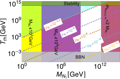
Figure 5: The allowed region (unshaded area) on $(T_{\rm rh},M_{N_{1}})$ plane and viable range for the Yukawa-like coupling $y_{N_{1}}$ to produce the baryon asymmetry of the present universe for NMPQ in metric formalism for the benchmark (m)BM3.

The value of $Y_{B}$ from Planck2018 data can be obtained as Rubakov and Gorbunov (2017); Co et al. (2022)

$$Y_{B}\equiv\frac{n_{B}-n_{\bar{B}}}{s}=\frac{n_{\gamma}}{s}\eta_{B}=\simeq 8.7\times 10^{-11}$$ (71)

where $n_{B}-n_{\bar{B}}$, $n_{\gamma}$, and $\eta_{B}$ are difference in the number density of baryons and anti-baryons, the number density of CMB photons, and baryon-to-photon ratio, respectively. In Eq. 71, we use the values of present day number density of photons $n_{\gamma}\sim 410.73\,\,\text{cm}^{-3}$, and present day value of entropy density $s=2891.2\,\,\text{cm}^{-3}$ (as we are using $k_{B}=1$ unit) obtained from Planck2018 data. Utilizing Eqs. 67 and 71, we get for both metric and Palatini formalisms as

$$T_{\rm rh}\simeq 5.6073\times 10^{9}\,y_{N_{1}}^{2}\,{M_{N}}_{1}\,.$$ (72)

Here, we consider $\delta_{eff}=0.5$, and $m_{\nu_{3}}\approx 0.05\times 10^{-9}\,\text{GeV}$. Thus, if the sterile neutrino is produced from the decay of inflaton during the reheating era, and becomes accountable for the generation of baryon asymmetry of the present universe, then it must satisfy Eq. 72. These are presented as dotted lines for different values of $y_{N_{1}}$ in Fig. 5. In this plot, the unshaded region represents the permissible parameter space on $(T_{\rm rh},M_{N_{1}})$ plane for benchmark (m)BM3. Constraints on this plane include: a forest-green horizontal stripe situated at the top of the plot, representing the maximum permissible $T_{\rm rh}$ value; a cyan-colored wedge-shaped region in the upper-left corner. Both of these bounds are derived from Table 4. Additionally, a copper-rose vertical stripe on the right side reflects the condition $M_{N_{1}}$can not be $>{{m_{b}}}_{(m),\xi}/2$, while a slate-gray horizontal stripe at the bottom rules out the possibility $T_{\rm rh}<4\,\text{MeV}$. These constraints have been discussed in the context of Fig. 4. Furthermore, purple-colored region excludes $M_{N_{1}}<10^{9}\,\text{GeV}$ Davidson and Ibarra (2002), and a yellow-colored region similarly eliminates $M_{N_{1}}<10^{3}\,\text{GeV}$. Hence, for $10^{-3.5}\gtrsim y_{N_{1}}\gtrsim 10^{-12}$, the sterile neutrino produced from the decay of inflaton within the metric formalism of our considered inflationary scenario can effectively account for the entire baryon asymmetry in the present universe.

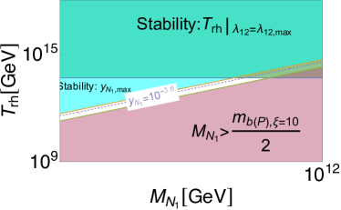
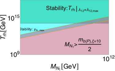
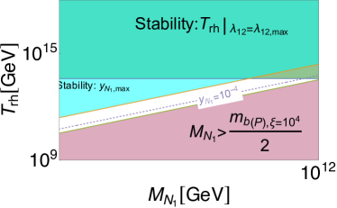
Figure 6: The allowed region (unshaded area) on $(T_{\rm rh},M_{N_{1}})$ plane and viable range for the Yukawa-like coupling $y_{N_{1}}$ to produce the baryon asymmetry of the present universe for NMPQ in Palatini formalism: top-left-panel for the benchmark (P)BM3 for $\upzeta=1$(top-left), top-right-panel is also for the benchmark (P)BM3 but for $\upzeta=10$, and bottom-panel is for the benchmark (P)BM7 and for $\upzeta=10$. Thus, the parameter space of $y_{N_{1}}$ within Palatini formalism is tightly constrained.

However, Palatini formalism puts more stringent bounds on the production of sterile neutrinos as it can be seen from Fig. 6. the bounds on this figures are : The maximum permissible value of $T_{\rm rh}$ obtained from the stability analysis in Table 5 i.e. $\left.T_{\rm rh}\right|_{\lambda_{12}=\lambda_{12,{\rm max}}}$. This is depicted as a forest-green horizontal stripe positioned at the top of the figures. The cyan-colored wedge-shaped area in the upper-left corner of the figures corresponds to the highest acceptable values of $y_{N_{1}}$ from Table 5. The presence of a copper-rose colored region effectively excludes the possibility of the value of $M_{N_{1}}$ surpassing ${{m_{b}}}_{(P),\xi}/2$. Top-left panel of Fig. 6 is for the benchmark (P)BM3 with $\upzeta=1$. For this scenario, the possibility of the sterile neutrino generated from inflaton decay contributing to baryon asymmetry is feasible only for $y_{N_{1}}\sim 10^{-3.6}$. Top-left panel of Fig. 6 is for the benchmark (P)BM3 with $\upzeta=10$, and this plot shows that the sterile neutrino from inflaton decay cannot account for the present-day baryon asymmetry within this scenario. However, the bottom panel reveals that successful Leptogenesis remains feasible for (P)BM7, even with $\upzeta=10$, if $y_{N_{1}}\sim 10^{-4}$.

VII Discussion and Conclusion

In this article, we considered slow-roll, single-field inflationary scenarios with quartic potential of the inflaton, and a non-minimal coupling between the inflaton and the gravity, and explored the particle production scenario from there-in. To this end, we suggested production of non-thermal fermionic BSM particle, which can be either stable or unstable, during the post-inflationary reheating era. Stable BSM fermionic particle can be accountable for the total CDM density of the universe. If the BSM fermionic particles are sterile neutrinos, they can decay to generate the total baryon asymmetry in the present universe via leptogenesis. Next, we studied a set of benchmark values for slow roll inflation satisfying bounds from CMB data within both metric and Palatini formalisms, and explored the corresponding parameter space of the coupling between the BSM fermionic field and inflaton, and the mass of the fermionic field that leads to successful DM relic and leads to observed baryon asymmetric of the universe. The salient features of our analysis are as follows:

• For our chosen benchmarks, the predicted values of $n_{s}$ and $r$ in both metric and Palatini formalisms, falls within $1-\sigma$ contour of combined analysis of Planck2018+Bicep3+Keck Array2018 on $(n_{s},r)$ plane for ${\cal N}_{\text{CMB}}\sim 60$ (see Fig. 1). For $\xi=0.5$, the predicted value of $r$ in Palatini formalism can be as small as $10^{-3}$, such that it can be tested in the future at $1-\sigma$ CL by forthcoming CMB-S4 experiment. We also observed from Tables 2 and 3, as well as from Fig. 2, that the difference between predicted values of $r$ in Palatini formalism and in metric formalism, for the same $\xi$, increases for higher values of $\xi$. This is because $r$ varies as $\xi^{-1}$. Left panel of Fig. 2 shows that increasing the value of $\xi$ and considering Palatini formulation of gravity helps to rescue the inflationary model, even when the predicted values of $r$ in metric formalism are invalidated by CMB observations.

• From stability analysis, we obtained the upper limit of the coupling between the inflaton and the BSM fermionic field as $<O(10^{-4})$ in both metric and Palatini formalisms. However, the upper limit of $\lambda_{12}$ obtained in metric formalism exceeds the value obtained in Palatini formalism by one order (see Tables 4 and 5).

• Since $m_{\phi}=0$ in both metric and Palatini formalisms, we suggested incorporating a bare mass term to the potential for successful reheating. From our estimation, we found that the upper limit of the bare mass term in metric formalism depends on $\xi$ (Eq. 37), whereas in Palatini formalism, it depends on $T_{\rm rh}$ (Eq. 38).

• In Fig. 3, we found that $T_{max}/T_{\rm rh}$ is higher in metric formalism than in Palatini formalism for same values of $\xi$ and ${\cal N}_{\text{CMB}}$. This is due to the fact that the inflaton potential around the minimum in Palatini formalism is quartic while it is quadratic around minimum in metric formalism. We also observed that $T_{max}/T_{\rm rh}$ differs noticeably with $\xi$ in Palatini formalism in contrast to metric formalism.

• From Fig. 4 we conclude that stable non-thermal $\chi$ produced only through inflaton decay can account for $100\%$ of the total relic density of CDM of the present universe, and the allowed range of $y_{\chi}$ is $10^{-3.5}\gtrsim y_{\chi}\gtrsim 10^{-20}$ in metric formalism, while $10^{-4}\gtrsim y_{\chi}\gtrsim 10^{-10}$ in Palatini formalism. Unlike metric formalism, we observed that the permissible range of $y_{N_{1}}$ varies noticeably with $\xi$ in Palatini formalism. Furthermore, in contrast to metric formalism, the permissible upper limit of $m_{\chi}$ depends on $T_{\rm rh}$, and the lower permissible value of $m_{\chi}$, derived by the Ly-$\alpha$ bound, is very low ($\sim{\cal O}\quantity(10^{-9})\,\text{GeV}$) in Palatini formalism, owing to the dependence of the upper limit of the bare mass on $T_{\rm rh}$. The benchmarks chosen for ${\cal N}_{\text{CMB}}\leavevmode\nobreak\ 60$ in metric formalism (Table 2) will be validated by future CMB observations, confirming the validity of the range of $y_{\chi}$ ($10^{-11}\gtrsim y_{\chi}\gtrsim 10^{-20}$). Additionally, CMB-S4 will affirm benchmarks in Palatini formalism, such as (P)BM3, indicating a valid range of $y_{\chi}$ around $10^{-11.5}$ for $\upzeta=10$. In summary, future CMB observations, such as CMB-S4, can confirm given scenarios for dark matter physics and matter-antimatter asymmetry in metric and Palatini formalisms, with respect to BSM parameters $y_{\chi}$ and $m_{\chi}$.

• When sterile neutrinos are produced from the decay of inflaton and generates total baryon asymmetry of the universe, we found from Fig. 5 that permissible range $y_{N_{1}}$ is $10^{-3.5}\gtrsim y_{N_{1}}\gtrsim 10^{-12}$ in metric formalism. However, Palatini formalism puts more stringent bounds on parameter space available for $y_{N_{1}}$. For instance, in the case of (P)BM3, generating the baryon asymmetry necessitates $y_{N_{1}}\sim 10^{-3.5}$ when bare mass is approximately equal to its upper limit. But there is no permissible range of $y_{N_{1}}$ when the bare mass is one order below the upper limit, or even smaller. This suggests that generating the universe’s total baryon asymmetry through leptogenesis involving sterile neutrinos produced from the decay of inflaton is severely constrained for our chosen inflationary scenario in Palatini formalism.

In summary, just by extending the standard model with two degrees of freedom: a real scalar inflaton, and a fermionic DM, we showed that tiny temperature fluctuations in CMBR can be explained via inflation and also addressed the the dark matter puzzle of the Universe. We have also made a comparative analysis between the metric and Palatini formalisms of gravity for the entire scenario. We have also demonstrated that future measurements of the CMB from experiments like CMB-S4, SPTpol, LiteBIRD, and CMB-Bharat Abazajian et al. (2016); Sayre et al. (2020); Hazumi et al. (2020); Adak et al. (2022) will further be able to test the simple models we have studied. We believe that, apart from producing necessary amount of DM and demonstrating successful Leptogenesis, starting from an well-motivated model of inflation in the two different gravity formalisms lead to different bounds on the parameter spaces thereby leaving significant effects on the corresponding physical conclusions of the theory. This is the major finding of the analysis, that makes it a compelling case to explore further.

As a future outlook we would like to analyze the scalar perturbations and see if large density fluctuations at small scales can occur in these models leading to PBH production and scalar-induced Gravitational Waves in upcoming GW experiments like Laser Interferometer Space Antenna (LISA), Cosmic Explorer, Einstein Telescope Amaro-Seoane et al. (2013); Evans et al. (2021); Maggiore et al. (2020). we leave such estimates for future studies.

Appendix A CW inflation

Since, we consider a SM gauge singlet BSM field as the inflaton with quartic potential in our work, the presence of self-interaction or Yukawa interaction in the Lagrangian density can give rise to quantum corrections. When such quantum loop corrections originating from interaction terms, UV completions Racioppi (2018), etc., are included, the effective potential for inflaton in Jordan frame becomes

$$V^{JF}(\varphi)=V_{\text{NMCW}}(\varphi)=\frac{\Lambda{\cal Q}^{4}}{4}+\Lambda\varphi^{4}\left[\log\left(\frac{\varphi}{{\cal Q}}\right)-\frac{1}{4}\right]\,,$$ (73)

where ${\cal Q}$ represents the renormalization scale, and the inclusion of the term $\frac{\Lambda{\cal Q}^{4}}{4}$ is to ensure that the value of the potential is $\gtrsim 0$, even at its minimum (the minimum of $V_{\text{NMCW}}(\varphi)$ is located at $\varphi={\cal Q}$). With an aim to find benchmark values for which predicted values of $(n_{s},r)$ fall within $1-\sigma$ best fit contour of Planck2018+Bicep3+Keck Array2015 combined analysis, unlike the form of non-minimal coupling considered in Eq. 2, we consider the non-minimal coupling of the following form Maji and Shafi (2023); Ghoshal et al. (2023d)

$$\Omega^{2}(\varphi)=1+\xi\frac{\varphi^{2}-{\cal Q}^{2}}{M_{P}^{2}}\,.$$ (74)

This particular form of non-minimal coupling also ensures that $\Omega^{2}(\varphi\to{\cal Q})\to 1$. Consequently, Einstein frame and Jordan frame becomes the same when inflaton reaches to the minimum of the potential. The potential for non-minimal Coleman Weinberg slow roll inflation (NMCW) in Einstein frame is

$$V^{E}(\varphi)\equiv V_{\text{NMCW}}^{E}(\varphi)=\frac{\frac{\Lambda{\cal Q}^{4}}{4}+\Lambda\varphi^{4}\left[\log\left(\frac{\varphi}{{\cal Q}}\right)-\frac{1}{4}\right]}{\left(1+\xi\frac{\varphi^{2}-{\cal Q}^{2}}{M_{P}^{2}}\right)^{2}}\,.$$ (75)

For the form of non-minimal coupling in Eq. 74, the relation between the inflaton in Einstein frame and $\varphi$ is

$$\derivative{\phi}{\varphi}=\begin{cases}\sqrt{\frac{\xi(6\xi+1)\varphi^{2}M_{P}^{2}-\xi{\cal Q}^{2}M_{P}^{2}+M_{P}^{4}}{\left(M_{P}^{2}+\xi(\varphi^{2}-{\cal Q}^{2})\right){}^{2}}}&\text{(in metric theory)}\,,\\ \sqrt{\frac{M_{P}^{2}}{\left(M_{P}^{2}+\xi(\varphi^{2}-{\cal Q}^{2})\right)}}&\text{(in Palatini theory)}\,.\end{cases}$$ (76)

A set of benchmark values for slow roll inflation with potential $V_{\text{NMCW}}^{E}(\varphi)$ in Einstein frame in metric and Palatini formalism are mentioned for ${\cal N}_{\text{CMB}}=50$ and ${\cal N}_{\text{CMB}}=60$ in Tables 6 and 7. From those tables, we see that $\absolutevalue{\xi}<1$ for our chosen benchmark values. In this scenario, slow roll inflation initiates near $\phi=0$ and inflaton moves towards higher value of $\phi$ as inflation progresses. The picture is opposite for slow roll inflation in plain quartic potential for inflaton, where the inflaton moves from larger to smaller values of inflaton during slow roll inflation. The predicted values of $(n_{s},r)$ fall within $1-\sigma$ best-fit contour of Planck+Bicep+Keck Array combined data for ${\cal N}_{\text{CMB}}=60$, which is similar to inflation with plain quartic potential of inflaton (see Tables 2 and 3). Therefore, hereafter, we consider only the benchmark values corresponding to ${\cal N}_{\text{CMB}}=60$ for further analysis. The predicted $(n_{s},r)$ values for benchmark (m)NM-CW1, (m)NM-CW3, (P)NM-CW1, and (P)NM-CW3 are shown in Fig. 7 along with present $1-\sigma$ and $2-\sigma$ contour from Planck and Planck+Bicep+Keck Array mission, along with prospective future reaches from forthcoming CMB observations as mentioned in Fig. 1. From this figure, we can see that for the same values of $\xi$ and ${\cal N}_{\text{CMB}}$ for our chosen set of benchmarks, there is no large difference between the predicted values of $(n_{s},r)$ in metric and Palatini formalisms. This is in contrast to what we observed for a simple quartic potential for inflation, as illustrated in Fig. 1. The reason for these almost similar predicted values of $(n_{s},r)$ is our choice of $\absolutevalue{\xi}<1$. Additionally, the chosen four benchmarks ((m)NM-CW1, (m)NM-CW3, (P)NM-CW1, and (P)NM-CW3) for ${\cal N}_{\text{CMB}}\sim 60$, can be confirmed in the future with the help of the three forthcoming CMB observations, the prospective future reaches of which are illustrated in Fig. 7.

Table 6: Benchmark values for NMCW inflationary model in metric formalism.

Benchmark	${\cal Q}/M_{P}$	$\xi$	$\varphi_{\rm end}/M_{P}$	${\cal N}_{\text{CMB}}$	$\varphi_{*}/M_{P}$	$n_{s}$	$r\times 10^{2}$	$\Lambda$
(m)NM-CW1	$52$	$-0.0020$	$50.7913$	$60$	$39.0185$	$0.9647$	$1.5708$	$9.4735\times 10^{-15}$
(m)NM-CW2				$50$	$39.8917$	$0.9595$	$2.2375$	$1.3815\times 10^{-14}$
(m)NM-CW3	$175$	$-0.0025$	$174.1685$	$60$	$161.9637$	$0.9655$	$0.6114$	$2.9743\times 10^{-15}$
(m)NM-CW4				$50$	$162.9510$	$0.9603$	$0.8765$	$\ 4.3037\times 10^{-15}$

Table 7: Benchmark values for NMCW inflationary model in Palatini formalism.

Benchmark	${\cal Q}/M_{P}$	$\xi$	$\varphi_{\rm end}/M_{P}$	${\cal N}_{\text{CMB}}$	$\varphi_{*}/M_{P}$	$n_{s}$	$r\times 10^{2}$	$\Lambda$
(P)NM-CW1	$52$	$-0.0020$	$50.7649$	$60$	$38.9338$	$0.9647$	$1.5332$	$9.2276\times 10^{-15}$
(P)NM-CW2				$50$	$39.8033$	$0.9595$	$2.1851$	$1.3456\times 10^{-14}$
(P)NM-CW3	$175$	$-0.0025$	$173.9785$	$60$	$161.2729$	$0.9655$	$0.5104$	$2.4699\times 10^{-15}$
(P)NM-CW4				$50$	$162.2357$	$0.9605$	$0.7321$	$3.5699\times 10^{-15}$

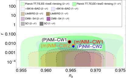
Figure 7: $(n_{s}-r)$ predictions for $\xi=-0.002$ and $\xi=-0.0025$ in both metric and Palatini formalism and for ${\cal N}_{\text{CMB}}\sim 60$ (from Tables 6 and 7) along with bounds on $(n_{s}-r)$ from current and future prospective reaches from forthcoming CMB observations mentioned in Fig. 1.

Table 8: Allowed range of $y_{\chi}$ and $\lambda_{12}$ for the benchmark values from Table 6.

Benchmark	stability for $y_{\chi}$		stability for $\lambda_{12}$
	about $\phi_{*}$	about $\phi_{\rm end}$	about $\phi_{*}$	about $\phi_{\rm end}$
(m)NM-CW1	$y_{\chi}<3.0956\times 10^{-4}$	$y_{\chi}<3.0671\times 10^{-4}$	$\lambda_{12}/M_{P}<2.3304\times 10^{-6}$	$\lambda_{12}/M_{P}<3.3615\times 10^{-6}$
(m)NM-CW3	$y_{\chi}<1.6355\times 10^{-4}$	$y_{\chi}<2.5870\times 10^{-4}$	$\lambda_{12}/M_{P}<8.9651\times 10^{-7}$	$\lambda_{12}/M_{P}<2.7832\times 10^{-6}$

Table 9: Allowed range of $y_{\chi}$ and $\lambda_{12}$ for the benchmark values from Table 7.

Benchmark	stability for $y_{\chi}$		stability for $\lambda_{12}$
	about $\phi_{*}$	about $\phi_{\rm end}$	about $\phi_{*}$	about $\phi_{\rm end}$
(P)NM-CW1	$y_{\chi}<3.0724\times 10^{-4}$	$y_{\chi}<3.0673\times 10^{-4}$	$\lambda_{12}/M_{P}<2.2859\times 10^{-6}$	$\lambda_{12}/M_{P}<3.3423\times 10^{-6}$
(P)NM-CW3	$y_{\chi}<1.5297\times 10^{-4}$	$y_{\chi}<2.5183\times 10^{-4}$	$\lambda_{12}/M_{P}<7.7185\times 10^{-7}$	$\lambda_{12}/M_{P}<2.5579\times 10^{-6}$

Following the similar approach used in Sec. IV, we estimated permissible upper values of $y_{\chi}$ and $\lambda_{12}$ for the interaction Lagrangian Eq. 12 and for $V^{E}_{\rm tree}\equiv V_{\text{NMCW}}^{E}(\varphi)$, and it is mentioned in Table 8 (for metric formalism) and in Table 9 (for Palatini formalism). From these table, we conclude that upper permissible values of $y_{\chi}$ and $\lambda_{12}$ are

• for (m)NM-CW1: $y_{\chi}<3.0671\times 10^{-4}$, $\lambda_{12}/M_{P}<2.3304\times 10^{-6}$.

• for (m)NM-CW3: $y_{\chi}<1.6355\times 10^{-4}$, $\lambda_{12}/M_{P}<8.9651\times 10^{-7}$.

• for (P)NM-CW1: $y_{\chi}<3.0673\times 10^{-4}$, $\lambda_{12}/M_{P}<2.2859\times 10^{-6}$.

• for (P)NM-CW3: $y_{\chi}<1.5297\times 10^{-4}$, $\lambda_{12}/M_{P}<7.7185\times 10^{-7}$.

These upper permissible values of $\lambda_{12}$ leads to the estimation of the maximum permissible value of $T_{\rm rh}$. We make the assumption that for NMCW inflation, reheating happens in quadratic potential for both metric and Palatini formalisms. Furthermore, $\varphi_{\rm min}={\cal Q}$ is the location of minimum of $V_{\text{NMCW}}^{E}(\varphi)$ and $m_{\phi}=\quantity(\left.\quantity({\differential^{2}V^{E}}/{\differential\phi^{2}})\right|_{\varphi=\varphi_{\rm min}})^{1/2}$ is not vanishing, as we have seen for plain quartic inflation (see Table 10). Hence, unlike NMPQ, we don’t require to introduce a bare mass term to the potential. The assumption that potential in Einstein frame around the minimum in NMCW inflation can be approximated as $\propto\phi^{2}$, even in Palatini formalism, along with non-vanishing values of $m_{\phi}$, leads to the different results in the context of DM production and leptogenesis, compared to NMPQ, that we obtain next for the production of DM and Leptogenesis.

Table 10: $m_{\phi}$ for NMCW inflationary model in both metric and Palatini formalism.

Benchmark	$m_{\phi}/M_{P}$
(m)NM-CW1	$9.8092\times 10^{-6}$
(m)NM-CW3	$1.3023\times 10^{-5}$
(P)NM-CW1	$9.9903\times 10^{-6}$
(P)NM-CW3	$1.7395\times 10^{-5}$

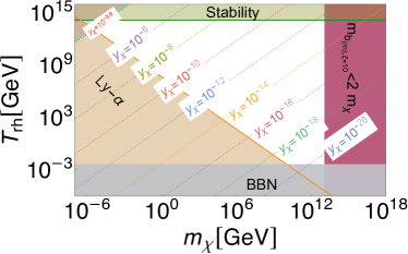
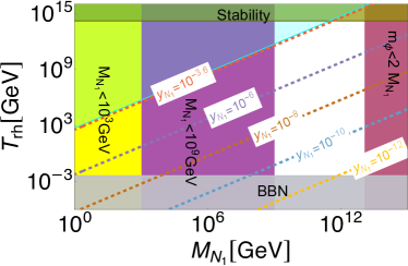
Figure 8: Left panel: shows the allowed region (unshaded area) on $(T_{\rm rh},m_{\chi})$ plane and viable range for the Yukawa-like coupling $y_{\chi}$ to produce the entire CDM density of the present universe. Right panel: displays the allowed region (unshaded area) on $(T_{\rm rh},M_{N_{1}})$ plane and viable range for the Yukawa-like coupling $y_{N_{1}}$ to produce the baryon asymmetry of the present universe. Both panels are for NMCW in metric formalism for the benchmark (m)NM-CW1. The allowed regions on $(T_{\rm rh},m_{\chi})$ plane and viable range for $y_{\chi}$, and allowed regions on $(T_{\rm rh},M_{N_{1}})$ plane and viable range of $y_{N_{1}}$ are almost identical for the benchmark (P)NM-CW1. This similarity arises from the almost identical values of $m_{\phi}$ and permissible upper limits of $y_{\chi}$ and $\lambda_{12}$, with slight variations, for both benchmarks (m)NM-CW1 and (P)NM-CW1.

Left panel of Fig. 8 is similar to Fig. 4, but for NMCW (benchmark - (m)NM-CW1). In this figure, the dashed lines correspond to Eq. 43 illustrating the values of $y_{\chi}$ for which $\chi$ produced from the decay of inflaton can be accountable for the $100\%$ of total CDM density of the present universe. The bounds on $(T_{\rm rh},m_{\chi})$ plane in Fig. 8 have been already mentioned in Fig. 4: from stability analysis mentioned in Table 8, $m_{\chi}$ should be $\lesssim m_{\phi}/2$ ($m_{\phi}$ is mentioned in Table 10), Ly-$\alpha$ bound from Eq. 52, BBN bound: $T_{\rm rh}\gtrsim 4\,\text{MeV}$. The allowed range of $y_{\chi}$ is $10^{-3.6}\gtrsim y_{\chi}\gtrsim 10^{-20}$, which is identical for metric formalism in NMPQ. In NMCW, the allowed range of $y_{\chi}$ is also nearly the same for Palatini formalism (benchmark (P)NM-CW1), because $m_{\phi}$, and the upper permissible limit of $y_{\chi}$ and $\lambda_{12}$ are almost identical in both metric and Palatini formalisms for our chosen benchmark values. Right panel of Fig. 8 is similar to Fig. 5, but for NMCW (benchmark - (m)NM-CW1) depicting allowed range for $y_{N_{1}}$ by dotted lines. The unshaded region is allowed, and the bound on $(T_{\rm rh},M_{N_{1}})$ plane have been already mentioned in Fig. 5. The allowed range of $y_{N_{1}}$ is $10^{-3.6}\gtrsim y_{N_{1}}\gtrsim 10^{-12}$, which is identical for metric formalism in NMPQ. The allowed region in Palatini formalism is identical and this conclusion is different from the result we obtained for NMPQ.

Appendix B Boltzmann

Here, we derive the expression for $T_{max}$ while reheating happens in either quadratic or quartic potential about the minimum. However, to make the calculations more general, we assume the potential during reheating $V^{E}\propto\phi^{k}$ where $k$ can be any even number $>0$ so that we can get a proper minimum during reheating. Then, the Boltzmann equations governing the evolution of $\rho_{\phi}$, $\rho_{\rm rad}$, and $\rho_{\chi}$ (which refers to energy density of $\chi$), and first Friedmann equation are given by Bernal et al. (2019); Giudice et al. (2001); Garcia et al. (2020)

$$\frac{\text{d}\rho_{\phi}}{\text{d}t}+3\left(\frac{2k}{k+2}\right){\cal H}\rho_{\phi}=-\Gamma_{\phi}\rho_{\phi}.$$ (77)

$$\frac{\text{d}\rho_{\rm rad}}{\text{d}t}+4{\cal H}\rho_{\rm rad}\;=\;\Gamma_{\phi}\rho_{\phi}\,,$$ (78)

$$\frac{\text{d}n_{\chi}}{\text{d}t}+3{\cal H}n_{\chi}\;=\;R(t)\,,$$ (79)

$${\cal H}^{2}\;=\;\frac{\rho_{\phi}+\rho_{\rm rad}+\rho_{\chi}}{3M_{P}^{2}}\;\approx\;\frac{\rho_{\phi}}{3M_{P}^{2}}\,,$$ (80)

The approximation presented in Eq. 80 holds true starting from the onset of reheating era and prior to the point when the temperature of SM relativistic plasma, or equivalently, the temperature of the universe reaches $T_{\rm rh}$. When $\Gamma_{\phi}\ll{\cal H}$, which occurs during the early stages of reheating, we can approximate the right-hand side of Eq. 77 as $0$. Under this approximation, the solution to Eq. 77 can be written as $\rho_{\phi}\propto\boldsymbol{a}^{-3\left(2k/(k+2)\right)}$. To further simplify the calculations of combined equations Eqs. 77, 78, 79 and 80, we make use of comoving energy density $\rho_{\phi}=R_{\phi}\,\boldsymbol{a}^{-3\left(2k/(k+2)\right)}$, $\rho_{\rm rad}\sim R_{\rm rad}\,\boldsymbol{a}^{-4}$, $\rho_{\chi}=R_{\chi}\,\boldsymbol{a}^{-3}$. By combining them with Eqs. 78 and 80, we obtain the following

$$\frac{\text{d}R_{\rm rad}}{\text{d}a}\;=\;\sqrt{3}M_{P}\,\Gamma_{\phi}\sqrt{R_{\phi}}\,\boldsymbol{a}^{6/(2+k)}\,,$$ (81)

which is applicable at early times i.e. when ${\cal H}\gg\Gamma_{\phi}$. This allows us to assume $R_{\phi}\approx R_{\phi_{I}}$, where $R_{\phi_{I}}$ is the value of $R_{\phi}$ at the beginning of reheating and $\frac{\text{d}R_{\phi_{I}}}{\text{d}\boldsymbol{a}}\approx 0$. Then

$$R_{\rm rad}\simeq\sqrt{3}M_{P}\,\Gamma_{\phi}\,\sqrt{R_{\phi_{I}}}\,\frac{2+k}{8+k}\boldsymbol{a}^{(8+k)/(2+k)}+\mathbb{c}$$ (82)

where $\mathbb{c}$ is the indefinite integral constant that may be settled with the assumption that

$$R_{\rm rad}(\boldsymbol{a}_{I})\simeq 0$$ (83)

Therefore,

$$R_{\rm rad}\simeq\sqrt{3}M_{P}\,\Gamma_{\phi}\,\sqrt{R_{\phi_{I}}}\,\frac{2+k}{8+k}\left(\boldsymbol{a}^{(8+k)/(2+k)}-\boldsymbol{a}_{I}^{(8+k)/(2+k)}\right)$$ (84)

To further facilitate the computations, let us introduce a variable $\boldsymbol{\mathcal{A}}\equiv\boldsymbol{a}/\boldsymbol{a}_{I}$. Besides, energy density of the produced relativistic SM particles which are thermalized and posses the temperature $T$ can be written as

$$R_{\rm rad}=\frac{\pi^{2}}{30}g_{\star}T^{4}\boldsymbol{\mathcal{A}}^{4}\boldsymbol{a}_{I}^{4}$$ (85)

Equating Eqs. 84 and 85, we obtain

$$T=3^{3/8}\left(\frac{10\,M_{P}\,\Gamma_{\phi}}{\pi^{2}\,g_{\star}}\sqrt{R_{\phi_{I}}}\right)^{1/4}\quantity(\frac{2+k}{8+k})^{1/4}\boldsymbol{a}_{I}^{\frac{-3k}{4(2+k)}}\left(\boldsymbol{\mathcal{A}}^{\frac{-3k}{(2+k)}}-\boldsymbol{\mathcal{A}}^{-4}\right)^{1/4}$$ (86)

In Eq. 86, the maximum value of $T$ can be obtained if $\left(\boldsymbol{\mathcal{A}}^{\frac{-3k}{(2+k)}}-\boldsymbol{\mathcal{A}}^{-4}\right)^{1/4}$ reaches maximum, which happens when

$$\boldsymbol{\mathcal{A}}_{\rm max}=\left(\frac{4}{3}\frac{k+2}{k}\right)^{\frac{k+2}{k+8}}=\left(\frac{4}{3}\frac{2}{w+1}\right)^{\frac{2}{5-3w_{\rm re}}}$$ (87)

The, the maximum possible temperature during reheating

$$T_{max}=\left(\frac{60}{\pi^{2}\,g_{\star}}\right)^{1/4}\,M_{P}^{1/4}\,\Gamma_{\phi}^{1/4}\,R_{\phi_{I}}^{1/8}\,\boldsymbol{a}_{I}^{-\frac{3k}{4(k+2)}}\,\frac{3^{1/8}}{2^{3/4}}\left(\left(\frac{27}{64}\right)^{\frac{k}{k+8}}\left(\frac{k}{k+2}\right)^{\frac{3k}{k+8}}\right)^{1/4}$$ (88)

$$T_{max}=\left(\frac{60}{\pi^{2}\,g_{\star}}\right)^{1/4}\,M_{P}^{1/2}\,\Gamma_{\phi}^{1/4}\,{{\cal H}_{I}}^{1/4}\,\frac{3^{5/8}}{2^{3/4}}\left(\left(\frac{27}{64}\right)^{\frac{k}{k+8}}\left(\frac{k}{k+2}\right)^{\frac{3k}{k+8}}\right)^{1/4}$$ (89)

Therefore,

$$\quantity(\frac{3}{8})^{2/5}\,\left(\frac{60}{g_{\star}\,\pi^{2}}\right)^{1/4}\quantity({\cal H}_{I}\,\Gamma_{\phi})^{1/4}\,M_{P}^{1/2}\,,\qquad\text{(for quadratic)}\,,$$ (90)

$$\quantity(\frac{3}{16})^{1/4}\,\left(\frac{60}{g_{\star}\,\pi^{2}}\right)^{1/4}\quantity({\cal H}_{I}\,\Gamma_{\phi})^{1/4}\,M_{P}^{1/2}\,,\qquad\text{(for quartic)}\,.$$ (91)

Since $\boldsymbol{\mathcal{A}}^{-1}<\boldsymbol{\mathcal{A}}^{\frac{-3k}{4(2+k)}}$ for $\boldsymbol{\mathcal{A}}>1$ and $k>1$, we can approximate Eq. 86 as

$$T\approx 3^{3/8}\left(\frac{10\,M_{P}\,\Gamma_{\phi}}{\pi^{2}\,g_{\star}}\sqrt{R_{\phi_{I}}}\right)^{1/4}\quantity(\frac{2+k}{8+k})^{1/4}\boldsymbol{a}_{I}^{\frac{-3k}{4(2+k)}}\,\boldsymbol{\mathcal{A}}^{\frac{-3k}{4(2+k)}}$$ (92)

From Eq. 92, we can see that $T\propto\boldsymbol{a}^{{-3k}/{4(2+k)}}$. Additionally, using $\rho_{\phi}=R_{\phi}\,\boldsymbol{a}^{-3\left(2k/(k+2)\right)}$, we see that $\rho_{\phi}\sim T^{8}$ and this functional dependence remains unchanged regardless of whether we consider a quadratic or quartic potential for the inflaton during reheating.

Appendix C Upper limit estimation for bare mass

In this section, we estimate the upper limit on the bare mass that can be incorporated into the potential of inflaton for successful reheating without disrupting the slow roll inflationary scenario. We assume that the potential of inflaton around its minimum during reheating (in Einstein frame, with $\phi$ as the inflaton in Einstein frame) can be approximated using one of the following forms:

$$\tilde{V}^{E}(\phi)\propto\begin{cases}\Lambda_{{\rm qud}}\,\phi^{2}\,,\\ \Lambda_{\rm qur}\,\phi^{4}\,,\end{cases}$$ (93)

where $\Lambda_{{\rm qud}},\Lambda_{{\rm qur}}$ are numerical factors. Our initial goal is to calculate the upper limit for the bare mass when reheating occurrs at the quartic minimum. By using Eq. 27 along with the relation $\rho_{\phi}\propto\boldsymbol{a}^{-3\quantity(1+w_{\rm re})}$, we obtain during the reheating era Garcia et al. (2020)

$$\rho_{\phi}\propto\boldsymbol{a}^{-4}\,.$$ (94)

Comparing Eqs. 93 and 94, we can say that amplitude of oscillation varies as (for quartic potential)

$$\phi\sim\boldsymbol{a}^{-1}\,.$$ (95)

Therefore, $m_{\phi}\sim\boldsymbol{a}^{-1}$ (as $m_{\phi}\sim\sqrt{\Lambda_{\rm qur}}\,\phi$), and $\Gamma_{\phi}\sim\boldsymbol{a}^{1}$. Additionally, ${\cal H}\sim\boldsymbol{a}^{-2}$ as ${\cal H}\sim\sqrt{\tilde{V}^{E}(\phi)}$.

Hence,

$$\frac{\Gamma_{\phi}}{{\cal H}}\propto\boldsymbol{a}^{3}\,.$$ (96)

Therefore, using $\Gamma_{\phi,{\rm rh}}\sim{\cal H}_{\rm rh}$, we get

$$\frac{\boldsymbol{a}_{\rm rh}}{\boldsymbol{a}_{\rm end}}\sim\left(\frac{{\cal H}_{\rm end}}{\Gamma_{\phi,{\rm end}}}\right)^{1/3}\,.$$ (97)

By using Eq. 95 in Eq. 97, we obtain

$$\phi_{\rm rh}\sim\phi_{\rm end}\left(\frac{\Gamma_{\phi,end}}{{\cal H}_{\rm end}}\right)^{1/3}\,.$$ (98)

Then, using ${\cal H}_{\rm end}\sim\sqrt{V(\phi_{\rm end})}/(\sqrt{3}M_{P})$,

$$\phi_{\rm rh}\sim\left(\frac{\sqrt{3}\,M_{P}}{\sqrt{\Lambda_{\rm qur}}}\Gamma_{\phi,{\rm end}}\,\phi_{\rm end}\right)^{1/3}\sim\left(\frac{\sqrt{3}\,M_{P}\,\lambda_{12}^{2}}{8\pi\,{\Lambda_{\rm qur}}}\right)^{1/3}\,.$$ (99)

where we have used $\Gamma_{\phi,{\rm end}}=\frac{\lambda_{12}^{2}}{8\pi\sqrt{\Lambda_{\rm qur}}\phi_{\rm end}}$. If we want to incorporate a bare mass term ${{m_{b}}}$ during quartic reheating, we need to satisfy the following condition Dimopoulos et al. (2018)

$${{m_{b}}} <\sqrt{\Lambda_{\rm qur}}\,\phi_{\rm rh}=\sqrt{\Lambda_{\rm qur}}\left(\frac{\sqrt{3}\,M_{P}\,\lambda_{12}^{2}}{8\pi\,{\Lambda_{\rm qur}}}\right)^{1/3}$$ (100)

For reheating happens in quadratic potential, the upper limit on bare mass can straightforwardly be estimated as

$${{m_{b}}}<\sqrt{\Lambda_{\rm qud}}$$ (101)

References

- Bambi and Dolgov (2015) C. Bambi and A. D. Dolgov, Introduction to Particle Cosmology, UNITEXT for Physics (Springer, 2015).
- Aghanim et al. (2020) N. Aghanim et al. (Planck), Astron. Astrophys. 641, A6 (2020), [Erratum: Astron.Astrophys. 652, C4 (2021)], arXiv:1807.06209 [astro-ph.CO] .
- Zyla et al. (2020) P. A. Zyla et al. (Particle Data Group), PTEP 2020, 083C01 (2020).
- Fields et al. (2020) B. D. Fields, K. A. Olive, T.-H. Yeh, and C. Young, JCAP 03, 010 (2020), [Erratum: JCAP 11, E02 (2020)], arXiv:1912.01132 [astro-ph.CO] .
- Steigman (2008) G. Steigman, JCAP 10, 001 (2008), arXiv:0808.1122 [astro-ph] .
- Cohen et al. (1998) A. G. Cohen, A. De Rujula, and S. L. Glashow, Astrophys. J. 495, 539 (1998), arXiv:astro-ph/9707087 .
- Sakharov (1967) A. D. Sakharov, Pisma Zh. Eksp. Teor. Fiz. 5, 32 (1967).
- Hawking (1974) S. W. Hawking, Nature 248, 30 (1974).
- Zeldovich (1976) Y. B. Zeldovich, Pisma Zh. Eksp. Teor. Fiz. 24, 29 (1976).
- Kuzmin et al. (1985) V. A. Kuzmin, V. A. Rubakov, and M. E. Shaposhnikov, Phys. Lett. B 155, 36 (1985).
- Shaposhnikov (1986) M. E. Shaposhnikov, JETP Lett. 44, 465 (1986).
- Shaposhnikov (1987) M. E. Shaposhnikov, Nucl. Phys. B 287, 757 (1987).
- Fukugita and Yanagida (1986) M. Fukugita and T. Yanagida, Phys. Lett. B 174, 45 (1986).
- Minkowski (1977) P. Minkowski, Phys. Lett. B 67, 421 (1977).
- Gell-Mann et al. (1979) M. Gell-Mann, P. Ramond, and R. Slansky, Conf. Proc. C 790927, 315 (1979), arXiv:1306.4669 [hep-th] .
- Yanagida (1979) T. Yanagida, Conf. Proc. C 7902131, 95 (1979).
- Mohapatra and Senjanovic (1980) R. N. Mohapatra and G. Senjanovic, Phys. Rev. Lett. 44, 912 (1980).
- Mohapatra (2004) R. N. Mohapatra, in SEESAW25: International Conference on the Seesaw Mechanism and the Neutrino Mass (2004) pp. 29–44, arXiv:hep-ph/0412379 .
- Workman et al. (2022) R. L. Workman et al. (Particle Data Group), PTEP 2022, 083C01 (2022).
- Bergstrom et al. (2013) L. Bergstrom, T. Bringmann, I. Cholis, D. Hooper, and C. Weniger, Phys. Rev. Lett. 111, 171101 (2013), arXiv:1306.3983 [astro-ph.HE] .
- Cuoco et al. (2018) A. Cuoco, J. Heisig, M. Korsmeier, and M. Krämer, JCAP 04, 004 (2018), arXiv:1711.05274 [hep-ph] .
- ATL (2022) (2022).
- Pedro (2023) R. Pedro (ATLAS), SciPost Phys. Proc. 12, 048 (2023).
- Giagu (2019) S. Giagu, Front. in Phys. 7, 75 (2019).
- Kamionkowski and Kosowsky (1999) M. Kamionkowski and A. Kosowsky, Ann. Rev. Nucl. Part. Sci. 49, 77 (1999), arXiv:astro-ph/9904108 .
- Ade et al. (2021) P. A. R. Ade et al. (BICEP, Keck), Phys. Rev. Lett. 127, 151301 (2021), arXiv:2110.00483 [astro-ph.CO] .
- Boubekeur et al. (2015) L. Boubekeur, E. Giusarma, O. Mena, and H. Ramírez, Phys. Rev. D 91, 103004 (2015), arXiv:1502.05193 [astro-ph.CO] .
- Bezrukov (2008) F. L. Bezrukov, in 15th International Seminar on High Energy Physics (2008) arXiv:0810.3165 [hep-ph] .
- Kallosh and Linde (2013) R. Kallosh and A. Linde, JCAP 06, 027 (2013), arXiv:1306.3211 [hep-th] .
- Hertzberg (2010) M. P. Hertzberg, JHEP 11, 023 (2010), arXiv:1002.2995 [hep-ph] .
- Capozziello et al. (2011) S. Capozziello, F. Darabi, and D. Vernieri, Mod. Phys. Lett. A 26, 65 (2011), arXiv:1006.0454 [gr-qc] .
- Kallosh et al. (2014) R. Kallosh, A. Linde, and D. Roest, Phys. Rev. Lett. 112, 011303 (2014), arXiv:1310.3950 [hep-th] .
- Järv et al. (2018) L. Järv, A. Racioppi, and T. Tenkanen, Phys. Rev. D 97, 083513 (2018), arXiv:1712.08471 [gr-qc] .
- Racioppi (2017) A. Racioppi, JCAP 12, 041 (2017), arXiv:1710.04853 [astro-ph.CO] .
- Cheong et al. (2022) D. Y. Cheong, S. M. Lee, and S. C. Park, JCAP 02, 029 (2022), arXiv:2111.00825 [hep-ph] .
- Bostan (2023) N. Bostan, JCAP 02, 063 (2023), arXiv:2209.02434 [astro-ph.CO] .
- Racioppi (2020) A. Racioppi, JHEP 21, 011 (2020), arXiv:1912.10038 [hep-ph] .
- Bauer and Demir (2008) F. Bauer and D. A. Demir, Phys. Lett. B 665, 222 (2008), arXiv:0803.2664 [hep-ph] .
- Borunda et al. (2008) M. Borunda, B. Janssen, and M. Bastero-Gil, JCAP 11, 008 (2008), arXiv:0804.4440 [hep-th] .
- Shaposhnikov et al. (2020) M. Shaposhnikov, A. Shkerin, and S. Zell, JCAP 07, 064 (2020), arXiv:2002.07105 [hep-ph] .
- Artymowski and Racioppi (2017) M. Artymowski and A. Racioppi, JCAP 04, 007 (2017), arXiv:1610.09120 [astro-ph.CO] .
- Kannike et al. (2016) K. Kannike, A. Racioppi, and M. Raidal, JHEP 01, 035 (2016), arXiv:1509.05423 [hep-ph] .
- Barrie et al. (2016) N. D. Barrie, A. Kobakhidze, and S. Liang, Phys. Lett. B 756, 390 (2016), arXiv:1602.04901 [gr-qc] .
- Allahverdi et al. (2010) R. Allahverdi, R. Brandenberger, F.-Y. Cyr-Racine, and A. Mazumdar, Ann. Rev. Nucl. Part. Sci. 60, 27 (2010), arXiv:1001.2600 [hep-th] .
- Ghoshal et al. (2023a) A. Ghoshal, Z. Lalak, and S. Porey, Phys. Rev. D 108, 063030 (2023a), arXiv:2302.03268 [hep-ph] .
- Ghoshal et al. (2022a) A. Ghoshal, G. Lambiase, S. Pal, A. Paul, and S. Porey, JHEP 09, 231 (2022a), arXiv:2206.10648 [hep-ph] .
- Asaka et al. (1999) T. Asaka, K. Hamaguchi, M. Kawasaki, and T. Yanagida, Phys. Lett. B 464, 12 (1999), arXiv:hep-ph/9906366 .
- Co et al. (2022) R. T. Co, Y. Mambrini, and K. A. Olive, Phys. Rev. D 106, 075006 (2022), arXiv:2205.01689 [hep-ph] .
- Senoguz and Shafi (2004) V. N. Senoguz and Q. Shafi, Phys. Lett. B 596, 8 (2004), arXiv:hep-ph/0403294 .
- Asaka et al. (2000) T. Asaka, K. Hamaguchi, M. Kawasaki, and T. Yanagida, Phys. Rev. D 61, 083512 (2000), arXiv:hep-ph/9907559 .
- Barrie et al. (2022) N. D. Barrie, C. Han, and H. Murayama, Phys. Rev. Lett. 128, 141801 (2022), arXiv:2106.03381 [hep-ph] .
- Bostan and Şenoğuz (2019) N. Bostan and V. N. Şenoğuz, JCAP 10, 028 (2019), arXiv:1907.06215 [astro-ph.CO] .
- Markkanen et al. (2018) T. Markkanen, T. Tenkanen, V. Vaskonen, and H. Veermäe, JCAP 03, 029 (2018), arXiv:1712.04874 [gr-qc] .
- Ferreira et al. (2018) R. Z. Ferreira, A. Notari, and G. Simeon, JCAP 11, 021 (2018), arXiv:1806.05511 [astro-ph.CO] .
- Ghoshal et al. (2023b) A. Ghoshal, M. Y. Khlopov, Z. Lalak, and S. Porey, (2023b), arXiv:2306.08675 [hep-ph] .
- AlHallak et al. (2022) M. AlHallak, N. Chamoun, and M. S. Eldaher, JCAP 10, 001 (2022), arXiv:2202.01002 [astro-ph.CO] .
- Park and Yamaguchi (2008) S. C. Park and S. Yamaguchi, JCAP 08, 009 (2008), arXiv:0801.1722 [hep-ph] .
- Rasanen and Wahlman (2017) S. Rasanen and P. Wahlman, JCAP 11, 047 (2017), arXiv:1709.07853 [astro-ph.CO] .
- Garcia-Bellido et al. (2009) J. Garcia-Bellido, D. G. Figueroa, and J. Rubio, Phys. Rev. D 79, 063531 (2009), arXiv:0812.4624 [hep-ph] .
- Bezrukov and Shaposhnikov (2009) F. Bezrukov and M. Shaposhnikov, JHEP 07, 089 (2009), arXiv:0904.1537 [hep-ph] .
- Bezrukov and Shaposhnikov (2008) F. L. Bezrukov and M. Shaposhnikov, Phys. Lett. B 659, 703 (2008), arXiv:0710.3755 [hep-th] .
- Ghoshal et al. (2022b) A. Ghoshal, G. Lambiase, S. Pal, A. Paul, and S. Porey, in 25th Workshop on What Comes Beyond the Standard Models? (2022) arXiv:2211.15061 [astro-ph.CO] .
- Ghoshal et al. (2023c) A. Ghoshal, G. Lambiase, S. Pal, A. Paul, and S. Porey, Symmetry 15, 543 (2023c).
- Bernal and Xu (2021) N. Bernal and Y. Xu, Eur. Phys. J. C 81, 877 (2021), arXiv:2106.03950 [hep-ph] .
- Ghoshal et al. (2023d) A. Ghoshal, M. Y. Khlopov, Z. Lalak, and S. Porey, (2023d), arXiv:2306.09409 [hep-ph] .
- Gialamas et al. (2023) I. D. Gialamas, A. Karam, T. D. Pappas, and E. Tomberg, (2023), arXiv:2303.14148 [gr-qc] .
- Takahashi and Tenkanen (2019) T. Takahashi and T. Tenkanen, JCAP 04, 035 (2019), arXiv:1812.08492 [astro-ph.CO] .
- Racioppi and Vasar (2022) A. Racioppi and M. Vasar, Eur. Phys. J. Plus 137, 637 (2022), arXiv:2111.09677 [gr-qc] .
- Kannike et al. (2017) K. Kannike, A. Racioppi, and M. Raidal, Nucl. Phys. B 918, 162 (2017), arXiv:1605.09378 [hep-ph] .
- Racioppi et al. (2022) A. Racioppi, J. Rajasalu, and K. Selke, JHEP 06, 107 (2022), arXiv:2109.03238 [astro-ph.CO] .
- Okada and Raut (2017) N. Okada and D. Raut, Eur. Phys. J. C 77, 247 (2017), arXiv:1509.04439 [hep-ph] .
- Baumann (2011) D. Baumann, in Theoretical Advanced Study Institute in Elementary Particle Physics: Physics of the Large and the Small (2011) pp. 523–686, arXiv:0907.5424 [hep-th] .
- Lyth and Liddle (2009) D. H. Lyth and A. R. Liddle, The Primordial Density Perturbation (2009).
- Ade et al. (2022) P. A. R. Ade et al. (BICEP/Keck), in 56th Rencontres de Moriond on Cosmology (2022) arXiv:2203.16556 [astro-ph.CO] .
- Campeti and Komatsu (2022) P. Campeti and E. Komatsu, Astrophys. J. 941, 110 (2022), arXiv:2205.05617 [astro-ph.CO] .
- Hazumi et al. (2020) M. Hazumi et al. (LiteBIRD), Proc. SPIE Int. Soc. Opt. Eng. 11443, 114432F (2020), arXiv:2101.12449 [astro-ph.IM] .
- Abazajian et al. (2016) K. N. Abazajian et al. (CMB-S4), (2016), arXiv:1610.02743 [astro-ph.CO] .
- Ade et al. (2019) P. Ade et al. (Simons Observatory), JCAP 02, 056 (2019), arXiv:1808.07445 [astro-ph.CO] .
- Coleman and Weinberg (1973) S. R. Coleman and E. J. Weinberg, Phys. Rev. D 7, 1888 (1973).
- Drees and Xu (2021) M. Drees and Y. Xu, JCAP 09, 012 (2021), arXiv:2104.03977 [hep-ph] .
- Lin (2023a) C.-M. Lin, (2023a), arXiv:2303.13008 [hep-ph] .
- Lin (2023b) C.-M. Lin, (2023b), arXiv:2305.01159 [hep-ph] .
- Ellis et al. (2015) J. Ellis, M. A. G. Garcia, D. V. Nanopoulos, and K. A. Olive, JCAP 07, 050 (2015), arXiv:1505.06986 [hep-ph] .
- Garcia et al. (2020) M. A. G. Garcia, K. Kaneta, Y. Mambrini, and K. A. Olive, Phys. Rev. D 101, 123507 (2020), arXiv:2004.08404 [hep-ph] .
- Bernal et al. (2019) N. Bernal, F. Elahi, C. Maldonado, and J. Unwin, JCAP 11, 026 (2019), arXiv:1909.07992 [hep-ph] .
- Giudice et al. (2001) G. F. Giudice, E. W. Kolb, and A. Riotto, Phys. Rev. D 64, 023508 (2001), arXiv:hep-ph/0005123 .
- Fong et al. (2012) C. S. Fong, E. Nardi, and A. Riotto, Adv. High Energy Phys. 2012, 158303 (2012), arXiv:1301.3062 [hep-ph] .
- Rubakov and Gorbunov (2017) V. A. Rubakov and D. S. Gorbunov, Introduction to the Theory of the Early Universe: Hot big bang theory (World Scientific, Singapore, 2017).
- Di Bari (2012) P. Di Bari, Contemp. Phys. 53, 315 (2012), arXiv:1206.3168 [hep-ph] .
- Buchmuller et al. (2005) W. Buchmuller, R. D. Peccei, and T. Yanagida, Ann. Rev. Nucl. Part. Sci. 55, 311 (2005), arXiv:hep-ph/0502169 .
- Davidson et al. (2008) S. Davidson, E. Nardi, and Y. Nir, Phys. Rept. 466, 105 (2008), arXiv:0802.2962 [hep-ph] .
- Trodden (2004) M. Trodden, eConf C040802, L018 (2004), arXiv:hep-ph/0411301 .
- del Aguila et al. (1990) F. del Aguila, L. Ametller, G. L. Kane, and J. Vidal, Nucl. Phys. B 334, 1 (1990).
- Fukuyama et al. (2005) T. Fukuyama, T. Kikuchi, and T. Osaka, JCAP 06, 005 (2005), arXiv:hep-ph/0503201 .
- Hamaguchi (2002) K. Hamaguchi, Cosmological baryon asymmetry and neutrinos: Baryogenesis via leptogenesis in supersymmetric theories, Other thesis (2002), arXiv:hep-ph/0212305 .
- Sravan Kumar and Vargas Moniz (2019) K. Sravan Kumar and P. Vargas Moniz, Eur. Phys. J. C 79, 945 (2019), arXiv:1806.09032 [hep-ph] .
- Davidson and Ibarra (2002) S. Davidson and A. Ibarra, Phys. Lett. B 535, 25 (2002), arXiv:hep-ph/0202239 .
- Sayre et al. (2020) J. T. Sayre et al. (SPT), Phys. Rev. D 101, 122003 (2020), arXiv:1910.05748 [astro-ph.CO] .
- Adak et al. (2022) D. Adak, A. Sen, S. Basak, J. Delabrouille, T. Ghosh, A. Rotti, G. Martínez-Solaeche, and T. Souradeep, Mon. Not. Roy. Astron. Soc. 514, 3002 (2022), arXiv:2110.12362 [astro-ph.CO] .
- Amaro-Seoane et al. (2013) P. Amaro-Seoane et al., GW Notes 6, 4 (2013), arXiv:1201.3621 [astro-ph.CO] .
- Evans et al. (2021) M. Evans et al., (2021), arXiv:2109.09882 [astro-ph.IM] .
- Maggiore et al. (2020) M. Maggiore et al., JCAP 03, 050 (2020), arXiv:1912.02622 [astro-ph.CO] .
- Racioppi (2018) A. Racioppi, Phys. Rev. D 97, 123514 (2018), arXiv:1801.08810 [astro-ph.CO] .
- Maji and Shafi (2023) R. Maji and Q. Shafi, JCAP 03, 007 (2023), arXiv:2208.08137 [hep-ph] .
- Dimopoulos et al. (2018) K. Dimopoulos, C. Owen, and A. Racioppi, Astropart. Phys. 103, 16 (2018), arXiv:1706.09735 [hep-ph] .