Goal Oriented Adaptive Space Time Finite Element Methods Applied to Touching Domains

Abstract

We consider goal-oriented adaptive space-time finite-element discretizations of the parabolic heat equation on completely unstructured simplicial space-time meshes. In some applications, we are interested in an accurate computation of some possibly nonlinear functionals at the solution, so called goal functionals. This motivates the use of adaptive mesh refinements driven by the dual-weighted residual (DWR) method. The DWR method requires the numerical solution of a linear adjoint problem that provides the sensitivities for the mesh refinement. This can be done by means of the same full space-time finite element discretization as used for the primal linear problem. The numerical experiment presented demonstrates that this goal-oriented, full space-time finite element solver efficiently provides accurate numerical results for a model problem with moving domains and a linear goal functional, where we know the exact value.

1 Introduction

We consider the following parabolic evolution equation on moving domains: find $u$ such that

$$\frac{\mathrm{d}}{\mathrm{d}t}u-\Delta_{x}u=0\ \text{in }Q,$$ (1)

$$\nabla_{x}u\cdot\mathbf{n}=0\ \text{on }\Sigma,\text{ and }u=u_{0}\ \text{ on }\Sigma_{0},$$ (2)

with the material derivative $\frac{\mathrm{d}}{\mathrm{d}t}=\partial_{t}+(v\cdot\nabla_{x})$, where $v=\partial_{t}\Phi$ and $\Phi$ describes the movement of the the domain(s), the spatial Laplacian $\Delta_{x}$, and $Q=\{(x,t)\vcentcolon t\in(0,T),\ x\in\Omega(t)\}$, $\Sigma=\{(x,t)\vcentcolon t\in(0,T),\ x\in\partial\Omega(t)\}$, $\Sigma_{0}=\{(x,0)\vcentcolon x\in\Omega(0)\}$, where $\Omega(t)=\{\Phi(x,t)\vcentcolon x\in\Omega\}$ for $t\in(0,T)$.

We are however not interested in the solution $u$ of (1)–(2), but instead in the value of a certain Quantity of Interest (QoI), which is typically represented by a possibly nonlinear functional $J(\cdot)$. The QoI is usually some localized object, e.g. the mean of $u$ over a certain subregion of $\Omega$ at a certain time $t$. This warrants the use of adaptive mesh refinement to reduce the overall computational cost when aiming for a sufficiently high local resolution of the QoI. The standard approach for the solution of this class of problems is the method of lines, where we perform semi-discretization in space and time separately, where the goal oriented adaptivity introduces additional challenges, e.g. we have to store the solution at all discretization points in time; see e.g. besier2010goal ; failer2018adaptive ; munoz2019explicit ; fischer2023adaptive and the references therein. One possible way to overcome this requires checkpoint techniques as presented in ThesisMeisrimel . In this paper, we instead treat time as just another variable and perform an all-at-once discretization of the complete space-time cylinder $Q$. While this increases the dimension of our problem by one, it also enables us to simultaneously refine in space and time, and we have by design access to the solution over the whole time interval. Moreover, since we know the movement of the spatial domain in advance, the space-time domain is fixed; see e.g. Fig. 1. For more details on goal oriented space-time adaptivity for parabolic evolution problems, see endtmayer2023goaloriented and the references therein.

Figure 1: Two dimensional space-time domain, with the spatial dimension on the $x$-axis, and the temporal dimension on the $y$-axis.

The rest of the paper is structured as follows: in Section 2, we formally introduce the model problem and the space-time finite element discretization. In Section 3 we recall basic properties for the goal oriented error estimation technique and apply it to the space-time problem. Finally, in Section 4, we present a numerical experiment in one space dimension.

2 The model problem and discretization

In this section, we briefly describe the model problem and the corresponding space-time finite element discretization.

2.1 The model problem

We now consider (1)–(2) for the configuration sketched in Fig. 1, i.e. we consider two separate domains $\Omega_{1}$ and $\Omega_{2}$, which move towards each other with constant velocity $v$. Upon contact at $t=t_{\mathrm{contact}}>0$, the movement stops and the domains stay in contact for a fixed period of time $t_{\mathrm{dur}}>0$ , after which they separate at time $t=t_{\mathrm{separate}}=t_{\mathrm{contact}}+t_{\mathrm{dur}}$ and move away from each other, again with constant velocity $v$. In this setting, the total time derivative can be written as $\frac{\mathrm{d}}{\mathrm{d}t}=\partial_{t}+v\,\partial_{x}$.

By standard arguments we obtain the following weak formulation from (1)–(2): Find $u\in Eu_{0}+U:=\{Eu_{0}+\psi:\psi\in U\}$ such that

$$\langle\frac{\mathrm{d}}{\mathrm{d}t}u,v\rangle+\langle\nabla_{x}u,\nabla_{x}v\rangle=\langle f,v\rangle\qquad\quad\forall v\in V,$$ (3)

where $U$ and $V$ are reflexive Banach-spaces. Here, $\langle\cdot,\cdot\rangle$ denotes the $V^{*}\times V$ duality product, and $Eu_{0}$ solves the problem: Find $Eu_{0}\in H^{1}(Q)$ such that

$$-\Delta Eu_{0}=0\text{ in }Q,\qquad\text{and}\quad Eu_{0}=u_{0}\text{ on }\Sigma_{0},\quad\text{and}\qquad\nabla Eu_{0}\cdot n=0\text{ on }\Sigma.$$

2.2 Discretization

Let us assume $Q$ is polytopic. We decompose the domain $Q$ into non-overlapping shape-regular simplicial finite elements $\Delta\in\mathcal{T}_{h}$. Then, we define the corresponding finite space

$$U_{h}=V_{h}=\{v_{h}\in S^{k}_{h}(\overline{Q}):v_{h}=0\text{ on }\Sigma_{0}\},$$ (4)

where $S^{k}_{h}(\overline{Q}):=\{v_{h}\in\mathcal{C}(\overline{Q}):v_{h}\in\mathbb{P}^{k}(\Delta)\}$ is nothing else but the standard finite element space with polynomial degree $k=1,2,3,\ldots$. Here, $\mathbb{P}^{k}(\Delta)$ describes the polynomials with degree $k$ on the element $\Delta$. This leads to a conforming discretization. With this we define the discretized problem as: Find $u_{h}\in E_{h}u_{0}+U_{h}$ such that

$$\langle\frac{\mathrm{d}}{\mathrm{d}t}u_{h},v_{h}\rangle+\langle\nabla_{x}u_{h},\nabla_{x}v_{h}\rangle=0\qquad\quad\forall v_{h}\in V_{h},$$ (5)

where $E_{h}$ is an extension operator into $S_{h}^{k}(Q)$, which evaluates $u_{0}$ at the essential space-time boundary $\Sigma_{0}$ and is zero everywhere else. Further information about the space-time discretization can be found in steinbach2015 .

3 Goal oriented error estimates

In many applications the solution itself is not of primary interest but one or several quantities of interest $J_{i}\vcentcolon Eu_{0}+U\to\mathbb{R}$ which are evaluated at the solution. In this work, we just consider one quantity of interest $J$. For multiple quantities of interest we refer to HaHou03 ; Ha08 ; EnWi17 ; EnLaNeiWoWi2020 ; EnLaWi18 . Here, our error estimator should estimate the error in our functional, i. e. $\eta_{h}\approx J(u)-J(u_{h})$. For this we use the DWR (dual weighted residual) method BeRa01 ; BaRa03 . In general, the DWR method requires the solution of the adjoint problem. However in endtmayer2023goaloriented , it was shown that just the solution of an discretized adjoint problem is required. The discretized adjoint is given by: Find $z_{h}\in W_{h}$ such that:

$$\langle\frac{\mathrm{d}}{\mathrm{d}t}v_{h},z_{h}\rangle+\langle\nabla_{x}v_{h},\nabla_{x}z_{h}\rangle=\langle J^{\prime}(u_{h}),v_{h}\rangle,\qquad\forall v_{h}\in W_{h},$$ (6)

where $u_{h}$ solves (5) and $J^{\prime}$ describes the Fréchet derivative of the goal functional $J$. For linear quantities of interest the derivative $J^{\prime}$ does not depend on the solution of the primal problem $u_{h}$. The space $W_{h}$ can be the finite element space $V_{h}$ introduced above or an enriched finite element space $V_{h}^{(2)}$ with the property $V_{h}\subset V_{h}^{(2)}\subset V$. In order to construct the error estimator as in endtmayer2023goaloriented , the solution of the enriched primal problem is necessary. The enriched primal problem is given by: Find $u_{h}^{(2)}\in V_{h}^{(2)}$ such that

$$\langle\frac{\mathrm{d}}{\mathrm{d}t}u_{h}^{(2)},v_{h}^{(2)}\rangle+\langle\nabla_{x}u_{h}^{(2)},\nabla_{x}v_{h}^{(2)}\rangle=\langle f,v_{h}^{(2)}\rangle\qquad\quad\forall v_{h}^{(2)}\in V_{h}^{(2)}.$$ (7)

Finally the resulting error estimator $\eta_{h}$ is given by

$$\eta_{h}:=\frac{1}{2}\rho(u_{h})(z_{h}^{(2)}-z_{h})+\frac{1}{2}\rho^{*}(u_{h},z_{h})(u_{h}^{(2)}-u_{h})+\rho(u_{h})(z_{h})+\mathcal{R}_{h}^{(3)(2)}.$$ (8)

This error estimator proofs to be efficient and reliable as shown in EnLaWi20 ; endtmayer2021reliability . In particular for our model problem the resulting terms look as follows:

$$\rho(u_{h})(e_{h}^{*}) =\langle f,e_{h}^{*}\rangle-\langle\frac{\mathrm{d}}{\mathrm{d}t}u_{h},e_{h}^{*}\rangle-\langle\nabla_{x}u_{h},\nabla_{x}e_{h}^{*}\rangle,$$

$$\rho^{*}(u_{h},z_{h})(e_{h}) =\langle J^{\prime}(u_{h}),e_{h}\rangle-\langle\frac{\mathrm{d}}{\mathrm{d}t}e_{h},z_{h}\rangle-\langle\nabla_{x}z_{h},\nabla_{x}e_{h}\rangle,$$

$$\rho(u_{h})(z_{h}) =\langle f,z_{h}\rangle-\langle\frac{\mathrm{d}}{\mathrm{d}t}u_{h},z_{h}\rangle-\langle\nabla_{x}u_{h},\nabla_{x}z_{h}\rangle,$$

$$\mathcal{R}_{h}^{(3)(2)} =\frac{1}{2}\int_{0}^{1}s(s-1)J^{\prime\prime\prime}(su_{h}^{(2)}+(1-s)u_{h})(e_{h},e_{h},e_{h})\mathrm{d}s,$$

where $J^{\prime\prime\prime}$ describes the 3rd Fréchet derivative, $e_{h}:=u_{h}^{(2)}-u_{h}$, and $e_{h}^{*}:=z_{h}^{(2)}-z_{h}$. Of course for linear goal functionals $\mathcal{R}_{h}^{(3)(2)}=0$ and $\rho(u_{h})(z_{h}^{(2)}-z_{h})=\rho^{*}(u_{h},z_{h})(u_{h}^{(2)}-u_{h})$. The localization is based on the partition of unity technique in RiWi15_dwr . For further details and information we refer to endtmayer2023goaloriented . The resulting adaptive space-time algorithm is summarized in Algorithm 1.

Algorithm 1 The adaptive space-time algorithm

1:repeat

2:     solve the primal and adjoint problem

3:     solve the enriched primal and adjoint problem

4:     compute the elementwise contributions via PU-technique

5:     select a set of marked elements $M$ using Dörfler marking Doerfler:1996a ,

6:     $\mathcal{T}_{k+1}\leftarrow\textsc{Refine}(\mathcal{T}_{k},M)$,

7:     $k\leftarrow k+1$,

8:until some stopping criterion is fulfilled.

4 Numerical experiments

Now let $Q=\mathring{\overline{M(\Omega_{1}\cup\Omega_{2})}}$ with $\Omega_{1}=(-2,-1)$ and $\Omega_{2}=(1,2)$, where

$$M(\Omega) :=\{m(x,t):x\in\Omega,t\in(0,T)\},$$

$$m(x,t) =\begin{cases}(x-\frac{20xt}{9|x|},t)&\ t<0.45,\\ (x+\frac{20xt}{9|x|}-\frac{20x}{9|x|},t)&\ t>0.55,\\ (x-\frac{x}{|x|},t)&\text{else}.\end{cases}$$

We visualized the domain $Q$ in Figure 1. We consider the following initial boundary value problem: find $u$ such that

$$\partial_{t}u(x,t)+v(x,t)\,\partial_{x}u(x,t)-\partial_{x^{2}}^{2}u(x,t)=0,(x,t)\in Q$$

$$\partial_{x}u(x,t)\,n_{x}=0,x\in\Sigma$$

$$u(x,0)=u_{0}(x),x\in{\Omega_{1}}\cup{\Omega_{2}}$$

where

$$v(x,t)=\begin{cases}\frac{20}{9}&x<0\ \text{and}\ t<0.45,\\ -\frac{20}{9}&x>0\ \text{and}\ t<0.45,\\ -\frac{20}{9}&x<0\ \text{and}\ t>0.55,\\ \frac{20}{9}&x>0\ \text{and}\ t>0.55,\\ 0&\text{else},\end{cases}\quad\text{and}\quad u_{0}(x)=\begin{cases}2&x\in\Omega_{1},\\ 0&\text{else}.\end{cases}$$

In order to test the adaptive Algorithm 1, we are interested in the following Quantity of Interest

$$J(u) \coloneqq\int_{1}^{2}\!u(x,T)\;\mathrm{d}x=g(t_{\mathrm{dur}})\approx$0.356\,823\,400\,452\,454\,042\,809\,470\,931\,381\,3$,$$

$$g(t_{\mathrm{dur}}) \coloneqq\frac{1}{\sqrt{\pi t_{\mathrm{dur}}}}\sum_{k=-\infty}^{\infty}\int_{-1}^{0}\int_{0}^{2}e^{-\frac{(x-4k-y)^{2}}{4t_{\mathrm{dur}}}}\,\mathrm{d}y\,\mathrm{d}x,$$

where $t_{\mathrm{dur}}$ is the duration of contact. The computational domain is modeled and meshed with gmshgmsh . We implemented Algorithm 1 in our own C++ code, based on the finite element library MFEM mfem:2021 . The linear systems are solved by means of the direct solver MUMPS mumps . The enriched finite element spaces for the goal oriented adaptivity are realized by increasing the polynomial degree of the ansatz functions by one. The set of marked triangles is refined using red-green refinement banksherman1981 . Unless stated otherwise, we use a marking threshold of $0.5$. We will express convergence rates by the convention $\mathcal{O}(h^{\alpha})=(N_{dofs})^{-\alpha/d}$.

Since there are no source terms present, we do not expect too much refinements for $t<t_{\mathrm{contact}}$. At time $t=t_{\mathrm{contact}}$, there is a singularity at the spatial origin $x=0$, which needs to be properly resolved. This singularity is equivalent to the singularity of a related initial boundary value problem which starts at $t=t_{\mathrm{contact}}$ and has discontinuous initial data, with the point of discontinuity at $x=0$. Hence we expect heavy refinements toward $(0,t_{\mathrm{contact}})$. Moreover, since our domain of interest is only on the “right” domain for $t>t_{\mathrm{separate}}$, we do not expect many refinements on the “left” domain for $t>t_{\mathrm{separate}}$.

In Figure 2, we present on the left side the convergence history of the error in the functional, i.e. $|J(u)-J(u_{h})|$, and on the right the efficiency index $\mathrm{I_{eff}}=\frac{|\eta_{h}|}{|J(u)-J(u_{h})|}$, for different polynomial degrees $k$. First, we note that uniform refinements always result in a rate of $\mathcal{O}(h)$, regardless of the polynomial degree. The polynomial degree only affects the constant. Applying Algorithm 1 with linear ansatz functions, i.e. $k=1$, we observe a convergence rate of $\mathcal{O}(h^{5/3})$, while simultaneously reducing the number of dofs needed to reach a certain error threshold by almost two orders of magnitude. In terms of efficiency, we observe that the efficiency index tends towards $\sim 0.9$. Increasing the polynomial degree to $k=2$ does improve the convergence behavior of the error in the goal functional to an observed rate of $\mathcal{O}(h^{13/6})$, but does not improve the efficiency index.

In Figure 3, we present the finite element solution $u_{h}$ and the adjoint solution (sensitivity) $z_{h}$, plotted over the mesh. We observe that the refinements concentrate on three main regions: the region around the contact singularity $(0,t_{\mathrm{contact}})$, the region around the separation point $(0,t_{\mathrm{separate}})$, and around our region of interest $\{(x,T)\vcentcolon 1<x<2\}$. We note that the refinements for $t<t_{\mathrm{contact}}$ on the right domain are on the one hand due to the closure step of the mesh refinement algorithm to preserve the quasi-uniformity, and on the other hand due to the loss of causality by using continuous-in-time ansatz functions. While the point of separation $(0,t_{\mathrm{separate}})$ is not a singularity for the primal problem, it acts as a singularity for the adjoint solution. The adjoint problem is formally a well posed backward heat equation, hence the point of separation appears as a contact point. The refinements towards the region of interest are as expected.

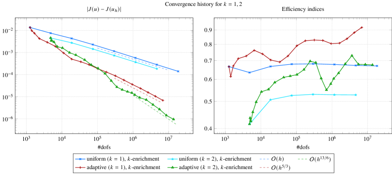
Figure 2: Convergence rates of the error in the functional and the corresponding efficiency index for the space-time domain with pre-contact part.

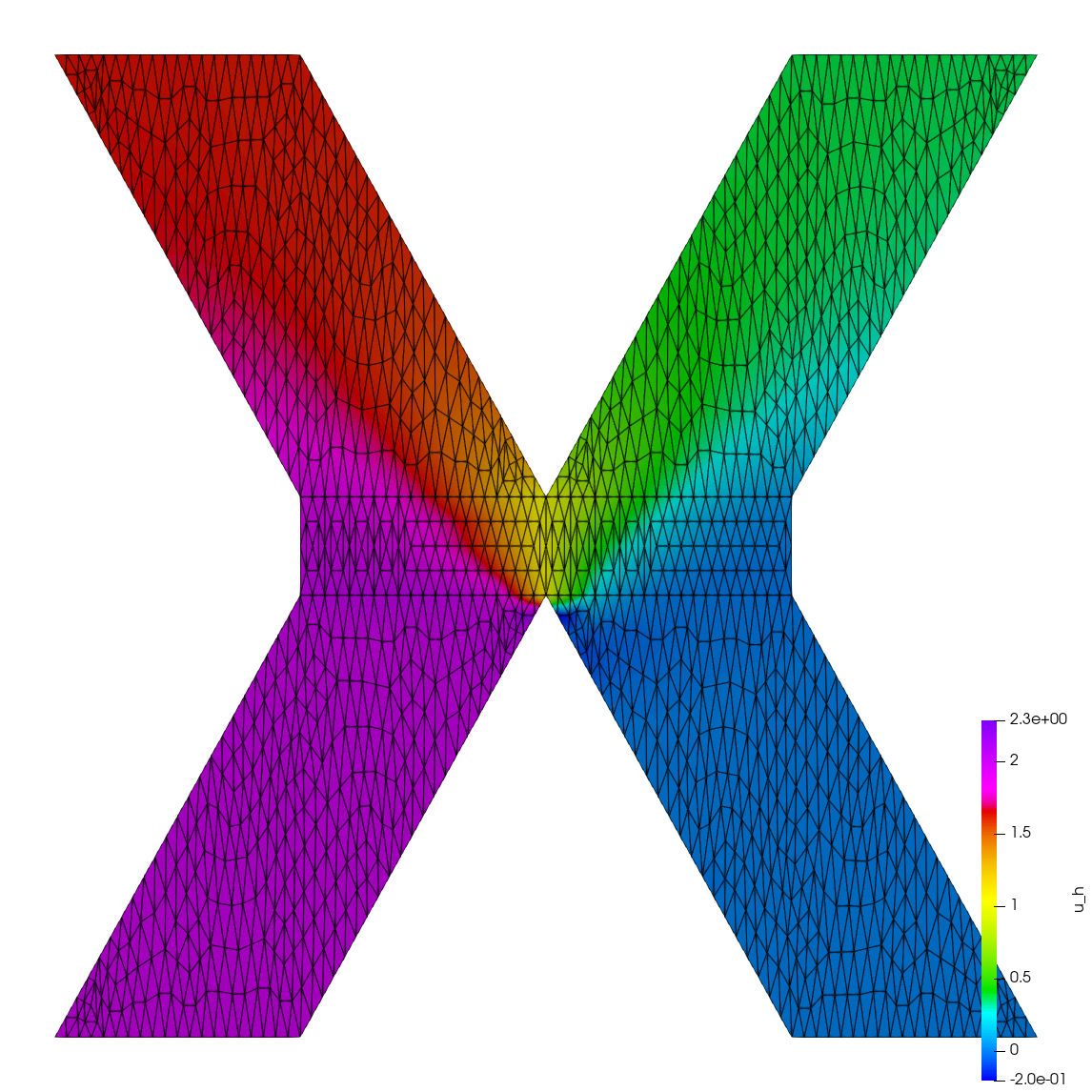
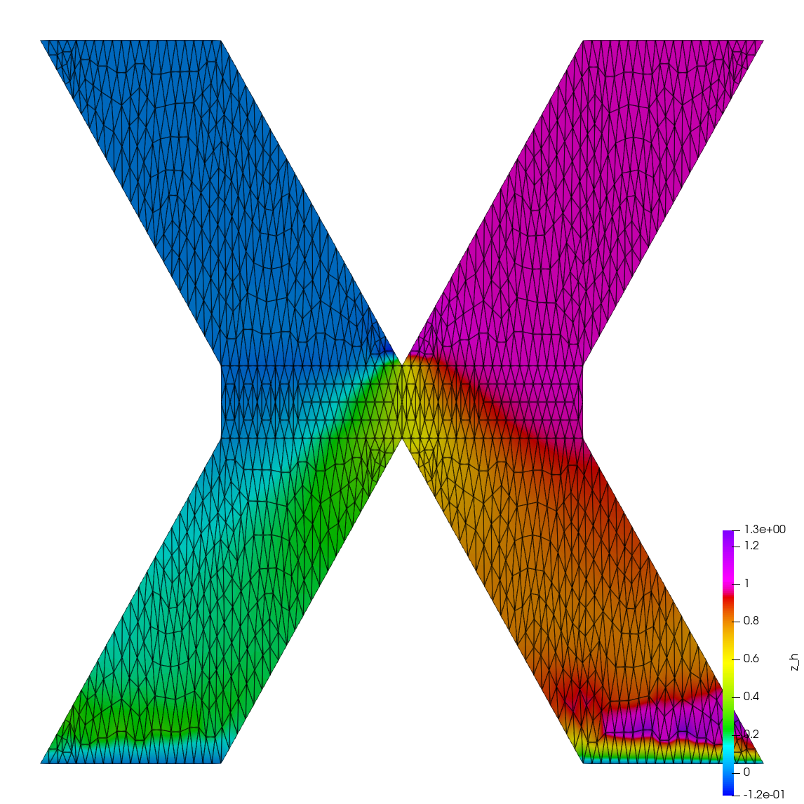
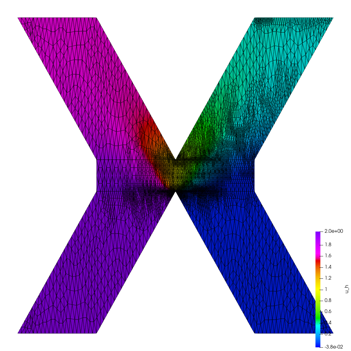
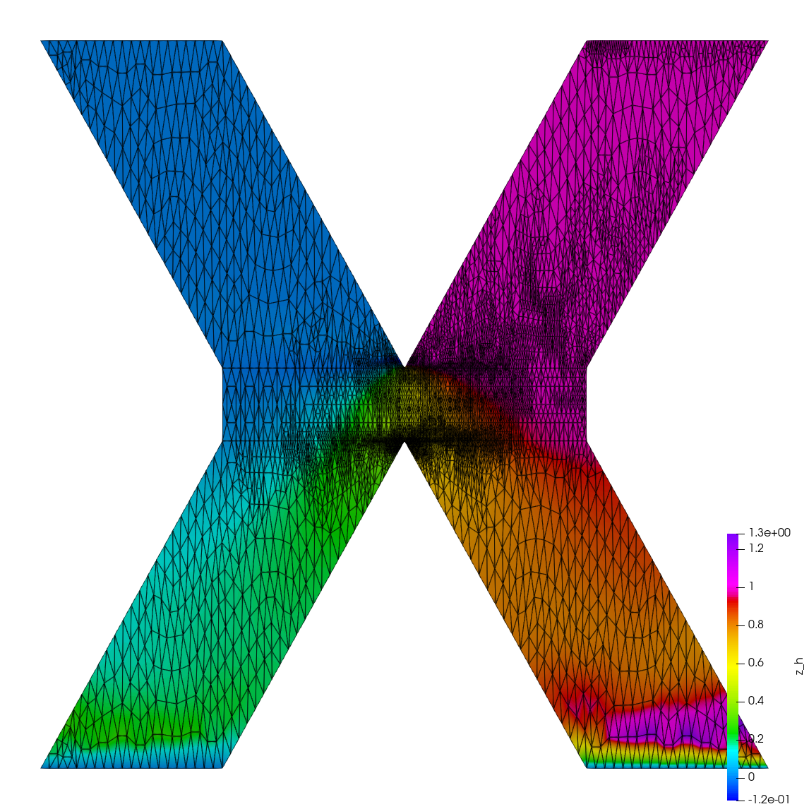
Figure 3: Initial space-time solution $u_{h}$ with mesh (upper left); initial space-time sensitivity $z_{h}$ with mesh (upper right); space-time solution $u_{h}$ with mesh after 5 adaptive refinements (lower left); space-time sensitivity $z_{h}$ with mesh after 5 adaptive refinements (lower right); using linear finite elements and $k$-enrichment for the DWR-estimator. The mesh was stretched in $t$-direction for visualization purposes only.

- (1) Amestoy, P.R., Duff, I.S., L’Excellent, J.Y., Koster, J.: A fully asynchronous multifrontal solver using distributed dynamic scheduling. SIAM J. Matrix Anal. Appl. 23(1), 15–41 (2001). DOI 10.1137/S0895479899358194
- (2) Anderson, R., Andrej, J., Barker, A., Bramwell, J., Camier, J.S., Dobrev, J.C.V., Dudouit, Y., Fisher, A., Kolev, T., Pazner, W., Stowell, M., Tomov, V., Akkerman, I., Dahm, J., Medina, D., Zampini, S.: MFEM: A modular finite element methods library. Computers & Mathematics with Applications 81, 42–74 (2021). DOI 10.1016/j.camwa.2020.06.009
- (3) Bangerth, W., Rannacher, R.: Adaptive Finite Element Methods for Differential Equations. Birkhäuser Verlag, Boston (2003)
- (4) Bank, R.E., Sherman, A.H.: An adaptive, multi-level method for elliptic boundary value problems. Computing 26, 91–105 (1981). DOI 10.1007/BF02241777
- (5) Becker, R., Rannacher, R.: An optimal control approach to a posteriori error estimation in finite element methods. Acta Numer. 10, 1–102 (2001)
- (6) Besier, M.: Goal-oriented adaptivity in space-time finite element simulations of nonstationary incompressible flows. Ph.D. thesis, University of Heidelberg (2010)
- (7) Dörfler, W.: A convergent adaptive algorithm for Poisson’s equation. SIAM J. Numer. Anal. 33(3), 1106–1124 (1996)
- (8) Endtmayer, B., Langer, U., Neitzel, I., Wick, T., Wollner, W.: Multigoal-oriented optimal control problems with nonlinear PDE constraints. Comput. Math. Appl. 79(10), 3001–3026 (2020). DOI 10.1016/j.camwa.2020.01.005
- (9) Endtmayer, B., Langer, U., Schafelner, A.: Goal-oriented adaptive space-time finite element methods for regularized parabolic p-laplace problems (2023). DOI 10.48550/arXiv.2306.07167
- (10) Endtmayer, B., Langer, U., Wick, T.: Multigoal-oriented error estimates for non-linear problems. J. Numer. Math. 27(4), 215–236 (2019)
- (11) Endtmayer, B., Langer, U., Wick, T.: Two-Side a Posteriori Error Estimates for the Dual-Weighted Residual Method. SIAM J. Sci. Comput. 42(1), A371–A394 (2020). DOI 10.1137/18M1227275
- (12) Endtmayer, B., Langer, U., Wick, T.: Reliability and efficiency of dwr-type a posteriori error estimates with smart sensitivity weight recovering. Computational Methods in Applied Mathematics 21(2), 351–371 (2021)
- (13) Endtmayer, B., Wick, T.: A Partition-of-Unity Dual-Weighted Residual Approach for Multi-Objective Goal Functional Error Estimation Applied to Elliptic Problems. Comput. Methods Appl. Math. 17(4), 575–599 (2017)
- (14) Failer, L., Wick, T.: Adaptive time-step control for nonlinear fluid–structure interaction. Journal of Computational Physics 366, 448–477 (2018)
- (15) Fischer, H., Roth, J., Chamoin, L., Fau, A., Wheeler, M.F., Wick, T.: Adaptive space-time model order reduction with dual-weighted residual (more dwr) error control for poroelasticity. arXiv preprint arXiv:2311.08907 (2023)
- (16) Geuzaine, C., Remacle, J.F.: Gmsh: a 3-D finite element mesh generator with built-in pre- and post-processing facilities. Int. J. Numer. Methods Eng. 79(11), 1309–1331 (2009). DOI 10.1002/nme.2579
- (17) Hartmann, R.: Multitarget error estimation and adaptivity in aerodynamic flow simulations. SIAM J. Sci. Comput. 31(1), 708–731 (2008). DOI 10.1137/070710962
- (18) Hartmann, R., Houston, P.: Goal-oriented a posteriori error estimation for multiple target functionals. In: Hyperbolic problems: theory, numerics, applications, pp. 579–588. Springer, Berlin (2003)
- (19) Meisrimel, P.: Adaptive time-integration for goal-oriented and coupled problems. Doctoral thesis (compilation), Faculty of Science (2021)
- (20) Muñoz-Matute, J., Calo, V.M., Pardo, D., Alberdi, E., van der Zee, K.G.: Explicit-in-time goal-oriented adaptivity. Computer Methods in Applied Mechanics and Engineering 347, 176–200 (2019)
- (21) Richter, T., Wick, T.: Variational localizations of the dual weighted residual estimator. J. Comput. Appl. Math. 279, 192–208 (2015). DOI 10.1016/j.cam.2014.11.008
- (22) Steinbach, O.: Space-time finite element methods for parabolic problems. Comput. Methods Appl. Math. 15(4), 551–566 (2015). DOI 10.1515/cmam-2015-0026