Ensemble Density-Functional Perturbation Theory: Spatial Dispersion in Metals

Abstract

We present a first-principles methodology, within the context of linear-response theory, that greatly facilitates the perturbative study of physical properties of metallic crystals. Our approach builds on ensemble density-functional theory [Phys. Rev. Lett. 79, 1337 (1997)] to write the adiabatic second-order energy as an unconstrained variational functional of both the wave functions and their occupancies. Thereby, it enables the application of standard tools of density-functional perturbation theory (most notably, the “$2n+1$” theorem) in metals, opening the way to an efficient and accurate calculation of their nonlinear and spatially dispersive responses. We apply our methodology to phonons and strain gradients and demonstrate the accuracy of our implementation by computing the spatial dispersion coefficients of zone-center optical phonons and the flexoelectric force-response tensor of selected metal structures.

I Introduction

In modern condensed matter physics, density-functional perturbation theory (DFPT) has emerged as the method of choice for accurately computing response properties of real materials. One key advantage that sets DFPT apart from alternative methods, e.g. the frozen-phonon technique [1], is its unique ability to handle incommensurate lattice distortions with arbitrary wave vectors $\mathbf{q}$ without significantly increasing the computational burden. Another important feature is related with the variational character of the Kohn-Sham energy functional: its perturbative expansion in powers of an adiabatic parameter $\lambda$ rests on the well-known $2n+1$ theorem, [2, 3, 4] enabling the calculation of, e.g., third-order response properties with the sole knowledge of first-order wave functions. Interestingly, by treating the wave vector $\mathbf{q}$ as an additional perturbation parameter, the advantages of the $2n+1$ theorem have recently been generalized to the long-wavelength expansion of the energy functional at an arbitrary order in the wave vector [5]. Successful application of long-wave DFPT techniques for the calculation of first-order spatial dispersion coefficients was demonstrated in several contexts, including flexoelectric coefficients [5, 6], dynamical quadrupoles [5, 6], natural optical activity [7] and generalized Lorentz forces [8].

In the context of DFPT, metals have historically been overshadowed by insulators. One of the main obstacles one needs to overcome when dealing with metals at zero temperature are Brillouin Zone (BZ) sampling errors coming from the Fermi surface discontinuities. The most effective and widely used strategy to deal with this issue at the ground-state level is the smearing technique [9]. In the latter approach, the sharp Fermi distribution, represented by the Heaviside step function, is approximated by a smoother function that is a broadened approximation of the former. The smearing approach was first introduced in the context of DFPT by de Gironcoli [10], thus enabling the computations of phonons in metals and, in turn, of a number of thermodynamic properties that depend on phonons and electron-phonon interactions (e.g., electrical and thermal conductivity, or superconductivity) [11]. In spite of its success, the formulation proposed by de Gironcoli lacks a straightforward variational formulation. This limitation prevents the application of the $2n+1$ theorem, which is key to accessing to higher-order energy derivatives.

The motivation for obtaining a theoretical framework that overcomes these obstacles is extensive, with notable emphasis on non-linear optics (NLO) [12, 13, 14, 15, 16, 17] and optical dispersion (OD) [18, 19, 20, 21, 22]. Apart from very few examples, most of the calculations that were reported insofar were based on semiclassical or tight-binding models. While these approaches can provide a reliable qualitative picture in many cases, their predictive power at the quantitative level is limited. As the experimental demand for reliable theoretical support is steadily growing in these areas, so is the need for a first-principles method that is free from the aforementioned drawbacks. A tentative roadmap towards this ambitious goal necessarily faces some of the long-standing technical obstacles that have slowed down progress in this area over the years: (i) Most first-principles attempts at calculating third-order (either nonlinear or spatially dispersive) coefficients have relied on cumbersome summations over a large number of unoccupied bands, with an obvious detrimental impact on both accuracy and computational efficiency. (ii) The effects of “local fields”, arising due to the self-consistent screening of the external perturbations have seldom been accounted for, even if their potentially dramatic impact on the response [23, 7] is known. (iii) Actual calculations are often plagued by the poorly conditioned nature of the dynamical response in a metal, where exceptional care in the computational parameters is often needed to avoid unphysical divergencies in the low-frequency limit.

In insulators, (i–ii) have been solved since the mid-90s, both at the static [24, 25] and dynamical [26] level, and (iii) does not pose any special issue as long as one works in the transparent regime. Addressing (i–iii) in metals appears as a daunting task, as they are all open problems in the context of the third-order response. As a first key step, in this work we shall focus on the issues (i–ii) in an adiabatic (static) context, and leave the additional complications related to the dynamical nature of the optical response to a future work. Note that, even within the adiabatic regime, a plethora of outstanding physical phenomena exists that require third-order energy derivatives for their correct treatment, e.g., phonon anharmonicity, nonlinear elasticity or force-response coefficients to strain gradients (flexocoupling coefficients, of relevance to the so-called ferroelectric metals [27]).

To enable their first-principles calculation, here we develop a general perturbative framework for metallic systems by using the ensemble density-functional theory formalism of Marzari, Vanderbilt and Payne (MVP) [28] as a conceptual basis. The invariance of the latter with respect to unitary transformations within the active subspace allows us to write an unconstrained second-order energy functional at an arbitrary $\mathbf{q}$ vector, which is stationary in the first-order wave functions and in the first-order occupation matrix. Then, mimicking the well-established procedure that is employed with insulators [5], the wave vector $\mathbf{q}$ is treated as a perturbation parameter, which provides (via the $2n+1$ theorem) an analytic long-wavelength expansion of the second-order energy functional at any desired order. Our methodology brings the first-principles calculation of dispersion properties in metals to the same level of accuracy and efficiency as in insulators, i.e., only the knowledge of uniform field perturbations is required to access first-order dispersion coefficients.

This work is organized as follows. In Sec. II.1 we summarize the fundamentals of ensemble density-functional theory as described in Ref. [28]. In Sec. II.2 we perform a perturbation expansion of the ensemble-DFT energy functional of MVP, obtaining an unconstrained second-order energy functional of the first-order orbitals and occupation matrices at an arbitrary wave vector $\mathbf{q}$. In Sec. III, following the guidelines of Ref. [5], we take the first-order long-wave expansion of the aforementioned second-order energy. In Sec. IV, we apply our general formalism to phonons and strain gradients, and validate our methodology by computing the spatial dispersion coefficients of zone-center phonons and the flexoelectric force-response tensor for a number of crystals, including the well-known ferroelectric metal LiOsO₃. Finally, we provide a brief summary and outlook in Sec. VI.

II Theory

II.1 Ensemble DFT

Here we recap the basics of ensemble DFT as formulated by Marzari, Vanderbilt and Payne [28], which can be regarded as a generalization of Mermin’s formulation of finite temperature DFT [29]. The key assumption of MVP consists in adopting a matrix representation for the occupancies ($f_{ij}$) via the following energy functional [28],

$$\begin{split}E[\{\psi_{m}\},\{f_{mn}\}]=&\sum_{m,n=1}^{M}f_{nm}\bra*{\psi_{m}}(\hat{T}+\hat{V}_{\text{ext}})\ket*{\psi_{n}}\\ &+E_{\text{Hxc}}[\rho]-\sigma S[\{f_{mn}\}]\\ &-\sum_{m,n=1}^{M}\Lambda_{mn}\left(\bra*{\psi_{m}}\ket*{\psi_{n}}-\delta_{mn}\right)\\ &-\mu\left(\Tr\left(\mathbf{f}\right)-N\right).\end{split}$$ (1)

Here $\hat{T}$ is the kinetic energy operator, $\hat{V}_{\text{ext}}$ refers to the atomic pseudopotentials and $E_{\text{Hxc}}$ is the Hartree exchange and correlation energy, which is a functional of the electron density,

$$\rho(\mathbf{r})=\sum_{m,n=1}^{M}f_{nm}\bra*{\psi_{m}}\ket*{\mathbf{r}}\bra*{\mathbf{r}}\ket*{\psi_{n}}.$$ (2)

In Eq. (1), $\sigma$ and $S$ are, respectively, the smearing parameter and the entropy. If the equilibrium distribution of the occupancies is chosen to follow the Fermi-Dirac (FD) statistics, $\sigma$ plays the role of a finite (electronic) temperature, $T$. In practice, using a smeared distribution function is primarily aimed at accelerating the convergence with $\mathbf{k}$-mesh density, so non-FD forms are often preferred [9, 30]. The Lagrange multipliers $\Lambda_{mn}$ and $\mu$ enforce the orthonormality of the wave functions and the particle number conservation, where $N$ is the total number of electrons. Sums are carried out for a number $M$ of active bands with nonzero occupancies. As long that the occupancies of the highest energy states within this active subspace ($\mathcal{M}$) are vanishingly small, further increasing $M$ does not produce any change in the total energy or in any other observable derived from Eq. (1).

If a diagonal representation for the occupation matrix ${\bf f}$ is enforced at all times, Eq. (1) reduces to the standard formulation [31, 32, 33] of Mermin’s approach. As the system evolves adiabatically in parameter space, however, the numerical integration of the resulting electronic equations of motion suffers from severe ill-conditioning issues. [32] Indeed, whenever level crossings occur near the Fermi surface, the orbitals need to abruptly change in character (via a subspace rotation) along the trajectory due to the explicit imposition of the Hamiltonian gauge. (Sharp symmetry-protected crossings are the most catastrophic, as they imply a discontinuity in the adiabatic evolution of the orbitals involved.) This is obviously not an issue in insulators, where the energy is invariant with respect to arbitrary unitary transformations within the occupied manifold.

The breakthrough idea of ensemble density-functional theory consists in allowing for nonzero off-diagonal elements of the occupation matrix ($f_{ij}$), and to treat them together with the wave functions ($\psi_{i}$) as variational parameters. By doing so, it is easy to prove that Eq. (1) is covariant under any unitary rotation $\mathbf{U}$ of the following type [28],

$$\begin{split}\quad\mathbf{f^{\prime}}&=\mathbf{UfU^{\dagger}},\\ \ket*{\psi_{m}}^{\prime}&=\sum_{n}U_{mn}^{\dagger}\ket*{\psi_{n}},\end{split}$$ (3)

which implies that one is no longer forced to stick to the Hamiltonian gauge. This way, the problematic [34, 35] subspace rotations can be conveniently reabsorbed into $f_{ij}$, which means that the first-order variations of the wave functions are automatically orthogonal to the active subspace, without the need of imposing additional constraints.

II.2 Perturbation expansion

In the following, we assume that the system under study evolves from its equilibrium state, which we describe by assuming a dependence of the Hamiltonian on some adiabatic parameter $\lambda$. In the perturbative regime, we write

$$\hat{H}(\lambda)=\hat{H}^{(0)}+\lambda\hat{H}^{(1)}+\frac{1}{2}\lambda^{2}\hat{H}^{(2)}+\dots$$ (4)

This parametric dependence propagates in a similar way to the wave functions and the occupation matrix,

$$\begin{split}\ket*{\psi_{m}(\lambda)}&=\ket*{\psi_{m}^{(0)}}+\lambda\ket*{\psi_{m}^{(1)}}+\dots,\\ f_{mn}(\lambda)&=f_{mn}^{(0)}+\lambda f_{mn}^{(1)}+\dots\end{split}$$ (5)

We now follow the guidelines of Refs. [3, 2] to recast the second-order energy as the constrained variational minimum of a functional that depends on both the first-order wave functions, $\ket*{\psi_{m}^{(1)}}$, and the first-order occupation matrix, $f_{mn}^{(1)}$. (In the next section we recast this problem as the minimization of an unconstrained energy functional, which poses great advantages in light of performing a long-wavelength expansion.) We find

$$\begin{split}E^{(2)}_{\text{con}}=&2\sum_{m,n=1}^{M}\left(f_{mn}^{(0)}\bra*{\psi_{n}^{(1)}}\hat{H}^{(0)}\ket*{\psi_{m}^{(1)}}-\Lambda^{(0)}_{mn}\bra*{\psi_{n}^{(1)}}\ket*{\psi_{m}^{(1)}}\right)+2\sum_{m,n=1}^{M}f_{mn}^{(0)}\left(\bra*{\psi_{n}^{(1)}}\hat{H}^{(1)}\ket*{\psi_{m}^{(0)}}+\text{c.c.}\right)\\ &+2\sum_{m,n=1}^{M}f_{mn}^{(1)}\bra*{\psi_{n}^{(0)}}\hat{H}^{(1)}\ket*{\psi_{m}^{(0)}}-\sigma\sum_{m,n,l,k=1}^{M}f_{mn}^{(1)}\frac{\partial^{2}S}{\partial f^{(0)}_{nm}\partial f^{(0)}_{lk}}f_{lk}^{(1)}\\ &+\int\int\rho^{(1)}(\mathbf{r})K_{\text{Hxc}}(\mathbf{r,r^{\prime}})\rho^{(1)}(\mathbf{r^{\prime}})d^{3}rd^{3}r^{\prime}+\sum_{m,n=1}^{M}f_{mn}^{(0)}\bra*{\psi_{n}^{(0)}}\hat{H}^{(2)}\ket*{\psi_{m}^{(0)}},\end{split}$$ (6)

where c.c. stands for complex conjugate and the Lagrange multipliers $\Lambda^{(0)}_{mn}$ are related to the matrix elements of the ground state Hamiltonian, $\Lambda^{(0)}_{mn}=f^{(0)}_{nm}\bra*{\psi_{m}^{(0)}}\hat{H}^{(0)}\ket*{\psi_{n}^{(0)}}$, with $f^{(0)}_{nm}=f_{m}\delta_{nm}$. (Note that the energy functional $E^{(2)}$ is defined as the second derivative of the total energy; this convention differs by a factor of two with respect to Refs. [5, 36, 2, 3].) The subscript “con” in Eq. (6) indicates that this energy functional is minimized subject to certain constraints. In this case, we impose that the ground-state wave functions are orthogonal to the first-order wave functions,

$$\bra*{\psi_{m}^{(0)}}\ket*{\psi_{n}^{(1)}}=0,\quad\forall m,n\in\mathcal{M},$$ (7)

which is also known as the parallel transport gauge [3]. We shall explain all the new terms appearing in Eq. (6) in the following. The second derivative of the entropy with respect to the occupation matrix appears in the second line of Eq. (6). By assuming a diagonal representation for the unperturbed occupation matrix, one can show that the following holds,

$$\sigma\frac{\partial^{2}S}{\partial f^{(0)}_{mn}\partial f^{(0)}_{kl}}=\frac{\delta_{mk}\delta_{nl}}{\bar{f}_{mn}},$$ (8)

where the matrix $\bar{f}_{mn}\equiv G(\epsilon_{m},\epsilon_{n})$ is defined as [35]

$$G(x,y)=\begin{cases}\frac{f(x)-f(y)}{x-y}&,\quad\text{if }x\neq y,\\[8.0pt] \frac{1}{2}\left(\frac{\partial f(x)}{\partial x}+\frac{\partial f(y)}{\partial y}\right)&,\quad\text{if }x=y.\end{cases}$$ (9)

(In the numerical implementation we set a finite tolerance to test the equality of $x$ and $y$, hence the need for the symmetrization in the second line; similar considerations apply to Eq. (55) later on.) The third line in Eq. (6) contains the Hartree exchange and correlation (Hxc) kernel,

$$K_{\text{Hxc}}(\mathbf{r,r^{\prime}})=\frac{\delta V_{\text{Hxc}}(\mathbf{r})}{\delta\rho(\mathbf{r^{\prime}})}=\frac{\delta^{2}E_{\text{Hxc}}}{\delta\rho(\mathbf{r})\delta\rho(\mathbf{r^{\prime}})},$$ (10)

and $\rho^{(1)}(\mathbf{r})$ is the first-order electron density, which depends both on the first-order wave functions as well as on the first-order occupation matrix,

$$\rho^{(1)}=\frac{\partial\rho}{\partial\psi}\psi^{(1)}+\frac{\partial\rho}{\partial f}f^{(1)}.$$ (11)

The stationary condition on the first-order occupation matrix allows us to find a solution for $f^{(1)}_{mn}$,

$$\frac{\delta E^{(2)}}{\delta f_{mn}^{(1)}}=0\longrightarrow f_{mn}^{(1)}=\bar{f}_{mn}\bra*{\psi_{m}^{(0)}}\mathcal{\hat{H}}^{(1)}\ket*{\psi_{n}^{(0)}},$$ (12)

where the calligraphic Hamiltonian indicates that SCF terms have been included, $\mathcal{\hat{H}}^{(1)}=\hat{H}^{(1)}+\hat{V}^{(1)}$, with

$$V^{(1)}(\mathbf{r})=\int K_{\text{Hxc}}(\mathbf{r,r^{\prime}})\rho^{(1)}(\mathbf{r^{\prime}})d^{3}r^{\prime}.$$ (13)

II.3 Unconstrained variational formulation

At this stage, in complete analogy with the insulating case [5] and with the forthcoming goal of performing a long-wavelength expansion of the energy functional, we can write an unconstrained variational functional for $E^{(2)}$ as follows,

$$\begin{split}E^{(2)}=&2\sum_{m=1}^{M}f_{m}\bra*{\psi_{m}^{(1)}}(\hat{H}^{(0)}+a\hat{P}-\epsilon_{m}^{(0)})\ket*{\psi_{m}^{(1)}}+2\sum_{m=1}^{M}f_{m}\left(\bra*{\psi_{m}^{(1)}}\hat{Q}\hat{H}^{(1)}\ket*{\psi_{m}^{(0)}}+\text{c.c.}\right)\\ &+2\sum_{m=1}^{M}f^{(1)}_{mn}\bra*{\psi_{n}^{(0)}}\hat{H}^{(1)}\ket*{\psi_{m}^{(0)}}-\sum_{m,n=1}^{M}f_{mn}^{(1)}\frac{\epsilon^{(0)}_{n}-\epsilon^{(0)}_{m}}{f_{n}-f_{m}}f^{(1)}_{nm}\\ &+\int\int\rho^{(1)}(\mathbf{r})K_{\text{Hxc}}(\mathbf{r,r^{\prime}})\rho^{(1)}(\mathbf{r^{\prime}})d^{3}rd^{3}r^{\prime}+\sum_{m}^{M}f_{m}\bra*{\psi_{m}^{(0)}}\hat{H}^{(2)}\ket*{\psi_{m}^{(0)}},\end{split}$$ (14)

where $a$ is a parameter with the dimension of energy that ensures the stability of the functional [5, 4] and the operators

$$\begin{split}\hat{P}=\sum_{m=1}^{M}\ket*{\psi_{m}^{(0)}}\bra*{\psi_{m}^{(0)}},\quad\hat{Q}=1-\hat{P},\end{split}$$ (15)

are projectors onto and out of the active subspace, respectively. These also are also relevant in the first-order electron density,

$$\begin{split}\rho^{(1)}(\mathbf{r})=&\sum_{m=1}^{M}f_{m}\bra*{\psi_{m}^{(1)}}\hat{Q}\ket*{\mathbf{r}}\bra*{\mathbf{r}}\ket*{\psi_{m}^{(0)}}+\text{c.c.}\\ &+\sum_{m,n=1}^{M}f^{(1)}_{mn}\bra*{\psi_{n}^{(0)}}\ket*{\mathbf{r}}\bra*{\mathbf{r}}\ket*{\psi_{m}^{(0)}}.\end{split}$$ (16)

(Note that, unlike in the insulating case, $\hat{P}$ does not correspond to the ground-state density operator.) The stationary condition on the first-order wave functions, $\delta E^{(2)}/\delta\bra*{\psi_{m}^{(1)}}=0$, leads to a standard Sternheimer equation, as proposed by Baroni et al. [4],

$$(\hat{H}^{(0)}+a\hat{P}-\epsilon_{m}^{(0)})\ket*{\psi_{m}^{(1)}}=-\hat{Q}\hat{\mathcal{H}}^{(1)}\ket*{\psi_{m}^{(0)}}.$$ (17)

II.4 Nonstationary formulas

Plugging the stationary conditions Eq. (12) and Eq. (17) into Eq. (14) results in the following nonstationary (nonst) expression for the second-order energy,

$$\begin{split}E^{(2)}_{\text{nonst}}=&\sum_{m=1}^{M}f_{m}\bra*{\psi_{m}^{(1)}}\hat{H}^{(1)}\ket*{\psi_{m}^{(0)}}+\text{c.c.}\\ &+\sum_{m,n=1}^{M}f_{mn}^{(1)}\bra*{\psi_{n}^{(0)}}\hat{H}^{(1)}\ket*{\psi_{m}^{(0)}}\\ &+\sum_{m=1}^{M}f_{m}\bra*{\psi_{m}^{(0)}}\hat{H}^{(2)}\ket*{\psi_{m}^{(0)}}.\end{split}$$ (18)

Interestingly, the only difference between Eq. (16) and Eq. (18) is that the first-order external perturbation, $\hat{H}^{(1)}$, appearing in the second-order energy is substituted with the operator $\ket*{\mathbf{r}}\bra*{\mathbf{r}}$ in the first-order electron density expression. We can even achieve a more compact version of the above by writing both the second-order energy and the first-order electron density as a trace,

$$E^{(2)}_{\text{nonst}}=\Tr\left(\hat{\rho}^{(1)}\hat{H}^{(1)}+\hat{\rho}^{(0)}\hat{H}^{(2)}\right)$$ (19)

and

$$\rho^{(1)}=\Tr\left(\hat{\rho}^{(1)}\ket*{\mathbf{r}}\bra*{\mathbf{r}}\right),$$ (20)

where the ground-state density operator is given by

$$\hat{\rho}^{(0)}=\sum_{m=1}^{M}\ket*{\psi_{m}^{(0)}}f_{m}\bra*{\psi_{m}^{(0)}},$$ (21)

and we have defined the first-order density operator as

$$\begin{split}\hat{\rho}^{(1)}=&\sum_{m=1}^{M}\ket*{\psi_{m}^{(0)}}f_{m}\bra*{{\psi}_{m}^{(1)}}+\text{c.c}\\ &+\sum_{m,n=1}^{M}\ket*{\psi_{m}^{(0)}}f^{(1)}_{mn}\bra*{\psi_{n}^{(0)}}.\end{split}$$ (22)

II.5 Relation to De Gironcoli’s approach

Our formalism naturally recovers De Gironcoli’s standard expressions for metals. We start by defining the following tilded first-order wave functions,

$$\begin{split}\ket*{\tilde{\psi}_{m}^{(1)}}=\ket*{\psi_{m}^{(1)}}+\frac{1}{2f_{m}}\sum_{n=1}^{M}\ket*{\psi_{n}^{(0)}}f^{(1)}_{mn}.\end{split}$$ (23)

The first-order density matrix is then given by

$$\hat{\rho}^{(1)}=\sum_{m=1}^{M}\ket*{\psi_{m}^{(0)}}f_{m}\bra*{\tilde{\psi}_{m}^{(1)}}+\text{c.c.},$$ (24)

which, in turn, exactly reduces to our Eq. (22). The nonstationary second-order energy and the first-order electron density can then be expressed succinctly using this notation as

$$\begin{split}E^{(2)}_{\text{nonst}}=&\sum_{m=1}^{M}f_{m}\bra*{\tilde{\psi}_{m}^{(1)}}\hat{H}^{(1)}\ket*{\psi_{m}^{(0)}}+\text{c.c.}\\ &+\sum_{m=1}^{M}f_{m}\bra*{\psi_{m}^{(0)}}\hat{H}^{(2)}\ket*{\psi_{m}^{(0)}}\end{split}$$ (25)

and

$$\rho^{(1)}=\sum_{m=1}^{M}f_{m}\bra*{\tilde{\psi}_{m}^{(1)}}\ket*{\mathbf{r}}\bra*{\mathbf{r}}\ket*{\psi_{m}^{(0)}}+\text{c.c.},$$ (26)

where this expression for the first-order electron density, Eq. (26), coincides with Eq. (10) of Ref. [10]. Our tilded first-order wave functions defined here can therefore be regarded as the $\Delta\phi_{i}(\mathbf{r})$ wave functions of de Gironcoli’s approach in Ref [10]. Interestingly, Eq. (25) and Eq. (26) resemble the expressions that are commonly used in insulators. Here, however, the tilded first-order wave functions take into account the subspace unitary rotations in the active subspace, via the second term on the right-hand side of Eq. (23); this term is absent in insulators.

II.6 Parametric derivative of operators

Eq. (22) can be regarded as special case of a more general rule for differentiating operators along adiabatic paths in parameter space. We establish this rule in the following, since it is key to the long-wave expansion of the second-order energy functional that we perform in the next section.

Consider an operator in the following form,

$$\hat{O}=\sum_{m=1}^{M}|\psi_{m}^{(0)}\rangle h(\epsilon^{(0)}_{m})\langle\psi_{m}^{(0)}|,$$ (27)

where $h(\epsilon^{(0)}_{m})$ is a real and differentiable function of the eigenvalue $\epsilon^{(0)}_{m}$. The derivative of $\hat{O}$ with respect to an adiabatic parameter $\lambda$ is then given by

$$\begin{split}\frac{\partial\hat{O}}{\partial\lambda}=&\sum_{m=1}^{M}\ket*{\psi_{m}^{(0)}}h(\epsilon^{(0)}_{m})\bra*{{\psi}_{m}^{\lambda}}+\text{c.c.}\\ &+\sum_{m,l=1}^{M}\mathcal{G}(\epsilon^{(0)}_{l},\epsilon^{(0)}_{m})|\psi_{m}^{(0)}\rangle\langle\psi_{m}^{(0)}|\mathcal{H}^{\lambda}|\psi_{l}^{(0)}\rangle\langle\psi_{l}^{(0)}|,\end{split}$$ (28)

where $\mathcal{G}$ is defined as in our Eq. (9), only replacing $f$ with $h$ therein. This result essentially corresponds to Eq. (20) of Ref. [15], but recast in an ensemble-DFPT form. Its proof rests on the following two rules,

$$\frac{\partial h(\epsilon^{(0)}_{m})}{\partial\lambda}= \frac{\partial h(\epsilon^{(0)}_{m})}{\partial\epsilon^{(0)}_{m}}\bra*{\psi_{m}^{(0)}}\hat{\mathcal{H}}^{\lambda}\ket*{\psi_{m}^{(0)}},$$ (29a)

$$\frac{\partial\ket*{\psi_{m}^{(0)}}}{\partial\lambda}= \ket*{\psi^{\lambda}_{m}}+\sum_{\begin{subarray}{c}n=1\\ n\neq m\end{subarray}}^{M}\frac{\bra*{\psi_{n}^{(0)}}\hat{\mathcal{H}}^{\lambda}\ket*{\psi_{m}^{(0)}}}{\epsilon_{m}^{(0)}-\epsilon_{n}^{(0)}},$$ (29b)

where the term $n=m$ is not included in the summation. Note that, when applied separately, Eq. (29) require that there be no degeneracies in the spectrum; conversely, Eq. (28) is valid in the general case. Whenever $h$ corresponds to the occupation function $f$, the operator $\hat{O}$ reduces to the ground-state density operator and Eq. (28) becomes Eq. (22).

III Long-wave expansion of the second-order energy functional

III.1 Monochromatic perturbations

We now apply the formalism presented in the previous subsection to the case of a monochromatic perturbation, modulated at a wave vector $\mathbf{q}$. By exploiting linearity, the first-order Hamiltonian is conveniently written as a phase times a cell-periodic part [36, 5], such that

$$\hat{H}^{(1)}(\mathbf{r,r^{\prime}})=e^{i\mathbf{q\cdot r}}\hat{H}_{\mathbf{q}}^{(1)}(\mathbf{r,r^{\prime}}),$$ (30)

and the Kohn-Sham wave functions are expressed as

$$\psi_{m\mathbf{k}}^{(0)}(\mathbf{r})=e^{i\mathbf{k\cdot r}}u_{m\mathbf{k}}^{(0)}(\mathbf{r}),$$ (31)

where $u_{m\mathbf{k}}^{(0)}(\mathbf{r})$ are the cell-periodic Bloch functions. We can now write the second-order energy functional as a stationary (st) functional (with respect to the wave functions and the occupation matrix) plus a nonvariational (nv) contribution,

$$E_{\mathbf{q}}^{\lambda_{1}\lambda_{2}}=E^{\lambda_{1}\lambda_{2}}_{\text{st},\mathbf{q}}+E^{\lambda_{1}\lambda_{2}}_{\text{nv},\mathbf{q}}.$$ (32)

For the sake of generality, we consider mixed derivatives with respect to two arbitrary perturbations, $\lambda_{1}$ and $\lambda_{2}$. (Applications to the specific cases of phonons and strains are discussed in Section IV.) The stationary part can be written as follows,

$$\begin{split}E^{\lambda_{1}\lambda_{2}}_{\text{st},\mathbf{q}}=&\int_{\text{BZ}}[d^{3}k]\left(\bar{E}_{\mathbf{k,q}}^{\lambda_{1}\lambda_{2}}+\bar{E}_{\mathbf{k+q,-q}}^{\lambda_{1}\lambda_{2}\,*}+\Delta E_{\mathbf{k,q}}^{\lambda_{1}\lambda_{2}}\right)\\ &+\int_{\Omega}\int\rho^{\lambda_{1}*}_{\mathbf{q}}(\mathbf{r})K_{\mathbf{q}}(\mathbf{r,r^{\prime}})\rho^{\lambda_{2}}_{\mathbf{q}}(\mathbf{r^{\prime}})d^{3}rd^{3}r^{\prime},\end{split}$$ (33)

where the shorthand notation $[d^{3}k]=\Omega/(2\pi)^{3}d^{3}k$ is used for the Brillouin Zone (BZ) integration and

$$K_{\mathbf{q}}(\mathbf{r,r^{\prime}})=K_{\text{Hxc}}(\mathbf{r,r^{\prime}})e^{i\mathbf{q}\cdot(\mathbf{r^{\prime}-r})}$$ (34)

is the phase-corrected Coulomb and exchange-correlation kernel. The second line of Eq. (33) explicitly depends on the first-order electron densities,

$$\begin{split}\rho_{\mathbf{q}}^{\lambda}(\mathbf{r})=\int_{\text{BZ}}[d^{3}k]\Bigg{[}&\sum_{m=1}^{M}\Big{(}f_{m\mathbf{k}}\bra*{u_{m\mathbf{k}}^{(0)}}\ket*{\mathbf{r}}\bra*{\mathbf{r}}\hat{Q}_{\mathbf{k+q}}\ket*{u_{m\mathbf{k,q}}^{\lambda}}\\ &+f_{m\mathbf{k+q}}\bra*{u_{m\mathbf{k+q,-q}}^{\lambda}}\hat{Q}_{\mathbf{k}}\ket*{\mathbf{r}}\bra*{\mathbf{r}}\ket*{u_{m\mathbf{k+q}}^{(0)}}\Big{)}\\ &+\sum_{m,n=1}^{M}\bra*{u_{m\mathbf{k}}^{(0)}}\ket*{\mathbf{r}}\bra*{\mathbf{r}}\ket*{u_{n\mathbf{k+q}}^{(0)}}f_{n\mathbf{k+q},m\mathbf{k}}^{\lambda}\Bigg{]},\end{split}$$ (35)

where $\ket*{u_{m\mathbf{k,q}}^{\lambda}}$ and $f_{n\mathbf{k+q},m\mathbf{k}}^{\lambda}$ are the first-order trial wave functions and occupation matrices, respectively. We shall name the new symbols appearing in Eq. (33) as the wave function ($\bar{E}$) and occupation ($\Delta E$) contributions, which are given by

$$\begin{split}\bar{E}^{\lambda_{1}\lambda_{2}}_{\mathbf{k,q}}=&\sum_{m=1}^{M}f_{m\mathbf{k}}\bra*{u_{m\mathbf{k,q}}^{\lambda_{1}}}(\hat{H}^{(0)}_{\mathbf{k+q}}+a\hat{P}_{\mathbf{k+q}}-\epsilon_{m\mathbf{k}}^{(0)})\ket*{u_{m\mathbf{k,q}}^{\lambda_{2}}}\\ &+\sum_{m=1}^{M}f_{m\mathbf{k}}\bra*{u_{m\mathbf{k,q}}^{\lambda_{1}}}\hat{Q}_{\mathbf{k+q}}\hat{H}^{\lambda_{2}}_{\mathbf{k,q}}\ket*{u_{m\mathbf{k}}^{(0)}}\\ &+\sum_{m=1}^{M}f_{m\mathbf{k}}\bra*{u_{m\mathbf{k}}^{(0)}}(\hat{H}^{\lambda_{1}}_{\mathbf{k,q}})^{\dagger}\hat{Q}_{\mathbf{k+q}}\ket*{u_{m\mathbf{k,q}}^{\lambda_{2}}},\end{split}$$ (36)

and

$$\begin{split}\Delta E^{\lambda_{1}\lambda_{2}}_{\mathbf{k,q}}=&\sum_{m,n=1}^{M}f^{\lambda_{1}}_{m\mathbf{k},n\mathbf{k+q}}\bra*{u_{n\mathbf{k+q}}^{(0)}}\hat{H}^{\lambda_{2}}_{\mathbf{k,q}}\ket*{u_{m\mathbf{k}}^{(0)}}\\ &+\sum_{m,n=1}^{M}\bra*{u_{m\mathbf{k}}^{(0)}}(\hat{H}^{\lambda_{1}}_{\mathbf{k,q}})^{\dagger}\ket*{u_{n\mathbf{k+q}}^{(0)}}f_{n\mathbf{k+q},m\mathbf{k}}^{\lambda_{2}}\\ &-\sum_{m,n=1}^{M}f^{\lambda_{1}}_{m\mathbf{k},n\mathbf{k+q}}\frac{\epsilon^{(0)}_{n\mathbf{k+q}}-\epsilon^{(0)}_{m\mathbf{k}}}{f_{n\mathbf{k+q}}-f_{m\mathbf{k}}}f^{\lambda_{2}}_{n\mathbf{k+q},m\mathbf{k}}.\end{split}$$ (37)

It is useful to recall the following Hermiticity conditions for first-order occupation matrices (${\bf f}^{\lambda}$) and operators ($\hat{H}^{\lambda}$, $\hat{\mathcal{H}}^{\lambda}$ or $\hat{\rho}^{\lambda}$),

$$f^{\lambda\dagger}_{n\mathbf{k+q},m\mathbf{k}}=f^{\lambda}_{m\mathbf{k},n\mathbf{k+q}},\qquad\hat{\rho}^{\lambda\dagger}_{\mathbf{k,q}}=\hat{\rho}^{\lambda}_{\mathbf{k+q,-q}},$$ (38)

which guarantees that the Fourier transform of the response functions defined here are real.

The stationary conditions on $\bra*{u^{\lambda_{1}}_{m\mathbf{k,q}}}$ and $f_{n\mathbf{k+q},m\mathbf{k}}^{\lambda_{1}\dagger}$ of this second-order energy functional give us the finite $\mathbf{q}$ counterparts of Eq. (12) and Eq. (17),

$$(\hat{H}^{(0)}_{\mathbf{k+q}}+a\hat{P}_{\mathbf{k+q}}-\epsilon_{m\mathbf{k}}^{(0)})\ket*{u^{\lambda_{2}}_{m\mathbf{k,q}}}=-\hat{Q}_{\mathbf{k+q}}\hat{\mathcal{H}}^{\lambda_{2}}_{\mathbf{k,q}}\ket*{u_{m\mathbf{k}}^{(0)}}$$ (39)

and

$$f^{\lambda_{2}}_{n\mathbf{k+q},m\mathbf{k}}=\frac{f_{n\mathbf{k+q}}-f_{m\mathbf{k}}}{\epsilon^{(0)}_{n\mathbf{k+q}}-\epsilon^{(0)}_{m\mathbf{k}}}\bra*{u_{n\mathbf{k+q}}^{(0)}}\hat{\mathcal{H}}^{\lambda_{2}}_{\mathbf{k,q}}\ket*{u_{m\mathbf{k}}^{(0)}}.$$ (40)

By plugging these two stationary conditions into the second-order energy functional, we obtain the following nonstationary expression,

$$E^{\lambda_{1}\lambda_{2}}_{\text{nonst},\mathbf{q}}=\int_{\text{BZ}}[d^{3}k]\,{\rm Tr}\left(\hat{H}^{\lambda_{1}}_{\mathbf{k+q,-q}}\hat{\rho}^{\lambda_{2}}_{\mathbf{k,q}}\right),$$ (41)

where the integrand is written in a compact form as a trace, and we have introduced the first-order density operator,

$$\begin{split}\hat{\rho}^{\lambda_{2}}_{\mathbf{k,q}}=&\sum_{m=1}^{M}\Big{(}\ket*{u_{m\mathbf{k,q}}^{\lambda_{2}}}f_{m\mathbf{k}}\bra*{u_{m\mathbf{k}}^{(0)}}\\ &+\ket*{u_{m\mathbf{k+q}}^{(0)}}f_{m\mathbf{k+q}}\bra*{u_{m\mathbf{k+q,-q}}^{\lambda_{2}}}\Big{)}\\ &+\sum_{m,n=1}^{M}\ket*{u_{n\mathbf{k+q}}^{(0)}}f^{\lambda_{2}}_{n\mathbf{k+q},m\mathbf{k}}\bra*{u_{m\mathbf{k}}^{(0)}}.\end{split}$$ (42)

As outlined in Sec. II.1, observable quantities must not depend on the size of the active subspace. It can be readily demonstrated that the second-order energy functional, $E^{\lambda_{1}\lambda_{2}}_{\text{nonst},\mathbf{q}}$, is independent of $M$. The proof relies on the $M$-independence of the first-order density operator, $\hat{\rho}^{\lambda_{2}}_{\mathbf{k,q}}$: if $M$ changes, part of the spectral weight is transferred from the first two lines to the Kubo-like term in the third line of Eq. (42), but the overall sum remains unchanged. In the limit where $M$ tends to infinity, the active space coincides with the entire Hilbert space; then, the first two lines vanish and the entire operator is expressed in a Kubo-like sum-over-all-states (third line in Eq. (42)) form [37]. Conversely, in gapped systems at zero temperature, it is common practice to resctrict the active subspace to its bare minimum (i.e., to the valence manifold). In this case $\Delta E^{\lambda_{1}\lambda_{2}}_{\mathbf{k,q}}$ vanishes identically, and the remainder contributions recover the well-known DFPT expressions for insulators [38, 4].

III.2 Time-reversal symmetry

The formulas presented in the previous subsection have the drawback that they require, in principle, to solve the Sternheimer problem simultaneously at ${\bf q}$ and ${\bf-q}$. In the following, we shall specialize our theory to crystals that enjoy time-reversal (TR) symmetry, where this inconvenience can be avoided. Indeed, assuming that both perturbations $\lambda_{1}$ and $\lambda_{2}$ are even under a TR operation, we have

$$\bra*{\mathbf{r}}\ket*{u_{m\mathbf{k}}^{(0)}}=\bra*{u_{m\mathbf{-k}}^{(0)}}\ket*{\mathbf{r}},\quad\bra*{\mathbf{r}}\ket*{u_{m\mathbf{k,q}}^{\lambda}}=\bra*{u_{m\mathbf{-k,-q}}^{\lambda}}\ket*{\mathbf{r}},$$ (43)

which implies

$$\bar{E}^{\lambda_{1}\lambda_{2}\,*}_{\mathbf{k+q,-q}}=\bar{E}^{\lambda_{1}\lambda_{2}}_{\mathbf{-k-q,q}}\rightarrow\bar{E}^{\lambda_{1}\lambda_{2}}_{\mathbf{k,q}}.$$ (44)

(Since the latter quantity must be anyway integrated over the Brillouin zone, we are allowed to operate an arbitrary shift in ${\bf k}$-space.) This allows us to write the stationary expression for the second derivative of the energy as

$$\begin{split}E^{\lambda_{1}\lambda_{2}}_{\text{st},\mathbf{q}}=&\int_{\text{BZ}}[d^{3}k]\left(2\bar{E}_{\mathbf{k,q}}^{\lambda_{1}\lambda_{2}}+\Delta E_{\mathbf{k,q}}^{\lambda_{1}\lambda_{2}}\right)\\ &+\int_{\Omega}\int\rho^{\lambda_{1}*}_{\mathbf{q}}(\mathbf{r})K_{\mathbf{q}}(\mathbf{r,r^{\prime}})\rho^{\lambda_{2}}_{\mathbf{q}}(\mathbf{r^{\prime}})d^{3}rd^{3}r^{\prime},\end{split}$$ (45)

with the first-order electron densities defined as

$$\begin{split}\rho_{\mathbf{q}}^{\lambda}(\mathbf{r})=\int_{\text{BZ}}[d^{3}k]\Bigg{[}&2\sum_{m=1}^{M}f_{m\mathbf{k}}\bra*{u_{m\mathbf{k}}^{(0)}}\ket*{\mathbf{r}}\bra*{\mathbf{r}}\hat{Q}_{\mathbf{k+q}}\ket*{u_{m\mathbf{k,q}}^{\lambda}}\\ &+\sum_{m,n=1}^{M}\bra*{u_{m\mathbf{k}}^{(0)}}\ket*{\mathbf{r}}\bra*{\mathbf{r}}\ket*{u_{n\mathbf{k+q}}^{(0)}}f_{n\mathbf{k+q},m\mathbf{k}}^{\lambda}\Bigg{]}.\end{split}$$ (46)

Note that the first-order wave functions at ${\bf-q}$ are no longer needed. After imposing the stationary principles, Eq. (39) and (40), we arrive at an analogous nonstationary formula for the second derivative,

$$\begin{split}E^{\lambda_{1}\lambda_{2}}_{\text{nonst},\mathbf{q}}=\int_{\text{BZ}}&[d^{3}k]\Bigg{[}2\sum_{m=1}^{M}f_{m\mathbf{k}}\bra*{u_{m\mathbf{k}}^{(0)}}(\hat{H}^{\lambda_{1}}_{\mathbf{k,q}})^{\dagger}\ket*{u_{m\mathbf{k,q}}^{\lambda_{2}}}\\ &+\sum_{m,n=1}^{M}\bra*{u_{m\mathbf{k}}^{(0)}}(\hat{H}^{\lambda_{1}}_{\mathbf{k,q}})^{\dagger}\ket*{u_{n\mathbf{k+q}}^{(0)}}f_{n\mathbf{k+q},m\mathbf{k}}^{\lambda_{2}}\Bigg{]}.\end{split}$$ (47)

The use of TR symmetry in DFPT is, of course, well established. The reason why we spell it out explicitly here is related to an important subtlety, specific to the metallic case, that is important to mention. The point is that, because of the shift in ${\bf k}$-space that we have operated on the TR-rectified “${\bf-q}$” terms, the integrands (i.e., the quantities in the square brackets) in Eq. (46) and (47) are no longer independent of $M$: such property is restored only after integration over the full BZ is performed. This observation has an undesirable consequence when operating the parametric differentiation in ${\bf q}$ (see next subsection): the accuracy of the result depends on the vanishing of the total ${\bf k}$-derivative of $\bar{E}_{\mathbf{k,0}}^{\lambda_{1}\lambda_{2}}$. For this requirement to hold, we need $\bar{E}_{\mathbf{k,0}}^{\lambda_{1}\lambda_{2}}$ to be a differentiable function of ${\bf k}$, which is only true if the active subspace forms an isolated group of bands (i.e., it must be separated from higher unoccupied states by a gap).

In all our test cases we were fortunate enough to find well-defined energy gaps in the conduction-band region of the spectrum, and we could always choose $M$ in such a way that $\epsilon^{(0)}_{M\mathbf{k}}-\epsilon^{(0)}_{M+1\mathbf{k}}\neq 0$ over the whole BZ. Less fortunate cases might require choosing a different $M$ for distinct $\mathbf{k}$ points, in order to avoid degeneracies between $M$ and $M+1$. (When such degeneracies are present, the linear-response Sternheimer problem becomes ill-conditioned, which makes it difficult or impossible to reach numerical convergence.) Although in principle possible, doing so would require using Eq. (33), in place of Eq. (45) as a starting point for the long-wave expansion. As this would entail a significant revision of the spatial-dispersion formulas already implemented in abinit, we defer such developments to a future work.

III.3 First-order in $\mathbf{q}$

In order to access spatial dispersion effects, our next task consists in taking the analytical derivative of Eq. (32) with respect to ${\bf q}$. Here the key advantage of our unconstrained variational formulation becomes clear, as it allows for a straightforward application of the $2n+1$ theorem. At first order, in particular, we have [5]

$$E^{\lambda_{1}\lambda_{2}}_{\gamma}=\frac{dE^{\lambda_{1}\lambda_{2}}_{\mathbf{q}}}{dq_{\gamma}}\bigg{|}_{\mathbf{q=0}}=\frac{\partial E^{\lambda_{1}\lambda_{2}}_{\mathbf{q}}}{\partial q_{\gamma}}\bigg{|}_{\mathbf{q=0}}.$$ (48)

This means that the total derivative in $\mathbf{q}$ coincides with the partial derivative of the second-order energy functional, where the variables that are implicitly defined by the stationary principle (in our case both the first-order wave functions, $\ket*{u^{\lambda}_{m\mathbf{k,q}}}$, and occupation matrices, $f^{\lambda}_{m\mathbf{k},n\mathbf{k+q}}$) are excluded from differentiation. In other words, the time-consuming self-consistent solution of the Sternheimer problem only needs to be performed at ${\bf q}=0$, just like in the insulating case. The only task we are left with consists in taking the derivatives of the nonvariational quantities in Eq. (33) that explicitly depend on ${\bf q}$, i.e., the external potentials and the ground-state wave functions. The final result for the ${\bf q}$-derivative of the stationary part reads as

$$\begin{split}E_{\text{st},\gamma}^{\lambda_{1}\lambda_{2}}=&\int_{\text{BZ}}[d^{3}k]\left(2\bar{E}_{\mathbf{k},\gamma}^{\lambda_{1}\lambda_{2}}+\Delta E_{\mathbf{k},\gamma}^{\lambda_{1}\lambda_{2}}\right)\\ &+\int_{\Omega}\int\rho^{\lambda_{1}*}(\mathbf{r})K_{\gamma}(\mathbf{r,r^{\prime}})\rho^{\lambda_{2}}(\mathbf{r^{\prime}})d^{3}rd^{3}r^{\prime},\end{split}$$ (49)

where

$$K_{\gamma}(\mathbf{r,r^{\prime}})=\frac{\partial K_{\mathbf{q}}(\mathbf{r,r^{\prime}})}{\partial q_{\gamma}}\Big{|}_{\mathbf{q=0}}$$ (50)

represents the first $\mathbf{q}$-gradient of the Hxc kernel. The wave-function term is in the exact same form as in the insulating case [5],

$$\begin{split}\bar{E}_{\mathbf{k},\gamma}^{\lambda_{1}\lambda_{2}}=&\sum_{m=1}^{M}f_{m\mathbf{k}}\bra*{u_{m\mathbf{k}}^{\lambda_{1}}}\hat{H}_{\mathbf{k}}^{k_{\gamma}}\ket*{u_{m\mathbf{k}}^{\lambda_{2}}}\\ &-\sum_{m,n=1}^{M}f_{m\mathbf{k}}\Big{(}\bra*{u_{m\mathbf{k}}^{\lambda_{1}}}\ket*{u_{n\mathbf{k}}^{k_{\gamma}}}\bra*{u_{n\mathbf{k}}^{(0)}}\hat{\mathcal{H}}_{\mathbf{k}}^{\lambda_{2}}\ket*{u_{m\mathbf{k}}^{(0)}}+\bra*{u_{m\mathbf{k}}^{(0)}}(\hat{\mathcal{H}}_{\mathbf{k}}^{\lambda_{1}})^{\dagger}\ket*{u_{n\mathbf{k}}^{(0)}}\bra*{u_{n\mathbf{k}}^{k_{\gamma}}}\ket*{u_{m\mathbf{k}}^{\lambda_{2}}}\Big{)}\\ &+\sum_{m=1}^{M}f_{m\mathbf{k}}\left(\bra*{u_{m\mathbf{k}}^{\lambda_{1}}}\hat{H}_{\mathbf{k},\gamma}^{\lambda_{2}}\ket*{u_{m\mathbf{k}}^{(0)}}+\bra*{u_{m\mathbf{k}}^{(0)}}(\hat{H}_{\mathbf{k},\gamma}^{\lambda_{1}})^{\dagger}\ket*{u_{m\mathbf{k}}^{\lambda_{2}}}\right),\end{split}$$ (51)

and the occupation term, specific to metals, reads as

$$\begin{split}\Delta E_{\mathbf{k},\gamma}^{\lambda_{1}\lambda_{2}}=&\sum_{m,n=1}^{M}\bar{f}_{mn\mathbf{k}}\left(\bra*{u_{m\mathbf{k}}^{(0)}}(\hat{\mathcal{H}}^{\lambda_{1}}_{\mathbf{k}})^{\dagger}\ket*{u_{n\mathbf{k}}^{(0)}}\bra*{u_{n\mathbf{k}}^{(0)}}\hat{H}_{\mathbf{k},\gamma}^{\lambda_{2}}\ket*{u_{m\mathbf{k}}^{(0)}}+\bra*{u_{m\mathbf{k}}^{(0)}}(\hat{H}_{\mathbf{k},\gamma}^{\lambda_{1}})^{\dagger}\ket*{u_{n\mathbf{k}}^{(0)}}\bra*{u_{n\mathbf{k}}^{(0)}}\hat{\mathcal{H}}_{\mathbf{k}}^{\lambda_{2}}\ket*{u_{m\mathbf{k}}^{(0)}}\right)\\ &+\sum_{m,n=1}^{M}\bar{f}_{mn\mathbf{k}}\left(\bra*{u_{m\mathbf{k}}^{(0)}}(\hat{\mathcal{H}}_{\mathbf{k}}^{\lambda_{1}})^{\dagger}\ket*{u_{n\mathbf{k}}^{(0)}}\bra*{u_{n\mathbf{k}}^{k_{\gamma}}}\hat{\mathcal{H}}_{\mathbf{k}}^{\lambda_{2}}\ket*{u_{m\mathbf{k}}^{(0)}}+\bra*{u_{m\mathbf{k}}^{(0)}}(\hat{\mathcal{H}}_{\mathbf{k}}^{\lambda_{1}})^{\dagger}\ket*{u_{n\mathbf{k}}^{k_{\gamma}}}\bra*{u_{n\mathbf{k}}^{(0)}}\hat{\mathcal{H}}_{\mathbf{k}}^{\lambda_{2}}\ket*{u_{m\mathbf{k}}^{(0)}}\right)\\ &+\sum_{m,n,l=1}^{M}\mathcal{F}_{mnl\mathbf{k}}\bra*{u_{m\mathbf{k}}^{(0)}}(\hat{\mathcal{H}}_{\mathbf{k}}^{\lambda_{1}})^{\dagger}\ket*{u_{n\mathbf{k}}^{(0)}}\bra*{u_{n\mathbf{k}}^{(0)}}\hat{H}_{\mathbf{k}}^{k_{\gamma}}\ket*{u_{l\mathbf{k}}^{(0)}}\bra*{u_{l\mathbf{k}}^{(0)}}\hat{\mathcal{H}}_{\mathbf{k}}^{\lambda_{2}}\ket*{u_{m\mathbf{k}}^{(0)}}.\end{split}$$ (52)

The proof of Eq. (52) rests on the rules for the differentiation of operators outlined in Sec. II.6, which we apply here to the case $\lambda=q_{\gamma}$ and $h(\epsilon^{(0)}_{m{\bf k+q}})=G(\epsilon^{(0)}_{n\bf k},\epsilon^{(0)}_{m{\bf k+q}})$.

The new symbols appearing in Eq. (51) and Eq. (52) are the $d/dk_{\gamma}$ wave functions, $\ket*{u_{m\mathbf{k}}^{k_{\gamma}}}$, the velocity operator,

$$\hat{H}_{\mathbf{k}}^{k_{\gamma}}=\frac{\partial\hat{H}_{\mathbf{k+q}}^{(0)}}{\partial q_{\gamma}}\Big{|}_{\mathbf{q=0}}$$ (53)

and

$$\hat{H}_{\mathbf{k},\gamma}^{\lambda}=\frac{\partial\hat{H}^{\lambda}_{\mathbf{k,q}}}{\partial q_{\gamma}}\Big{|}_{\mathbf{q=0}}.$$ (54)

The calligraphic symbol $\mathcal{F}_{mnl\mathbf{k}}\equiv\mathcal{F}(\epsilon_{m\mathbf{k}},\epsilon_{n\mathbf{k}},\epsilon_{l\mathbf{k}})$, which is invariant under any permutation of the three band indices, is defined as [35]

$$\mathcal{F}(x,y,z)=\begin{cases}\frac{G(x,y)-G(x,z)}{y-z},\quad y\neq z\\[8.0pt] \frac{1}{6}\left(\frac{\partial^{2}f(x)}{\partial x^{2}}+\frac{\partial^{2}f(y)}{\partial y^{2}}+\frac{\partial^{2}f(z)}{\partial z^{2}}\right),\quad x=y=z.\end{cases}$$ (55)

(See the parenthetical comment after Eq. (9).) We have carefully tested that our implementation of the function $\mathcal{F}(x,y,z)$ is continuous and smooth in the critical $x\simeq y\simeq z$ region. To illustrate the qualitative differences between $\mathcal{F}$ and $G$, in Fig. 1 we present two filled contour plots of the functions $G(x,y)$ and $\mathcal{F}(x,y,0)$: their respective symmetric and antisymmetric nature under the interchange of the two arguments is clear.

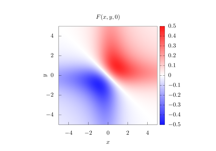
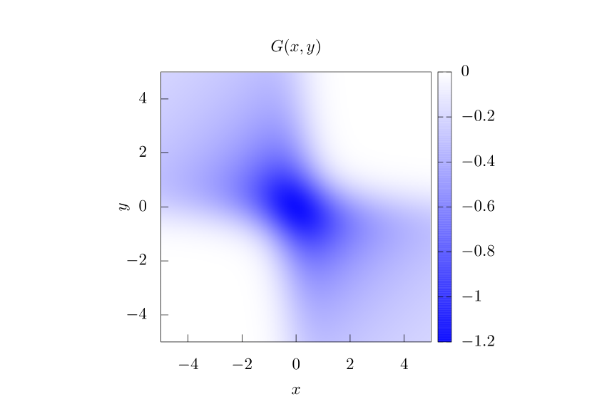
Figure 1: Two-dimensional contour plots (in arbitrary units) of the $\mathcal{F}$ and $G$ functions as defined in Eq. (55) and Eq. (9), respectively. The upper panel shows $\mathcal{F}(x,y,0)$ and the lower panel $G(x,y)$.

In close analogy to the finite-${\bf q}$ case, $\Delta E_{\mathbf{k},\gamma}^{\lambda_{1}\lambda_{2}}$ vanishes in insulators if the active manifold is restricted to the occupied states; the present formalism reduces then to the already established results [5].

III.4 Treatment of the $\mathbf{q}\rightarrow\mathbf{0}$ limit (Fermi level shifts)

Long-wave expansions generally require some care, as the Coulomb potential diverges in the ${\bf q}\rightarrow 0$ limit. In insulators, this divergence results in a nonanalytic contribution to the response that is due to long-range electric fields. In metals, such fields are screened by the redistribution of the free carriers, which tends to enforce local charge neutrality. The requirement of charge neutrality becomes strict at ${\bf q}=0$, where it needs to be taken care of explicitly, via the holonomic constraint on particle number in Eq. (1).

At second-order in the perturbations, this constraint propagates to the second-order energy functional as $\mu^{\lambda}\Tr(\mathbf{f^{\lambda}})$, where $\mu^{\lambda}$ plays the role of a first-order Lagrange multiplier [3]. By imposing the stationary condition on the $\mathbf{f^{\lambda}}$ matrix, one readily obtains the so-called “Fermi level shifts” contribution,

$$\begin{split}f^{\lambda}_{nm\mathbf{k}}&=\bar{f}_{nm\mathbf{k}}\left(\bra*{u^{(0)}_{n\mathbf{k}}}\hat{\mathcal{H}}^{\lambda}_{\mathbf{k}}\ket*{u^{(0)}_{m\mathbf{k}}}-\delta_{mn}\mu^{\lambda}\right)\\ &=\bar{f}_{nm\mathbf{k}}\bra*{u^{(0)}_{n\mathbf{k}}}\big{(}\hat{\mathcal{H}}^{\lambda}_{\mathbf{k}}-\mu^{\lambda}\big{)}\ket*{u^{(0)}_{m\mathbf{k}}}.\end{split}$$ (56)

A closed expression for $\mu^{\lambda}$ is can be obtained by imposing that the trace of $\mathbf{f}^{\lambda}$ should vanish,

$$\mu^{\lambda}=\frac{\displaystyle\int_{\text{BZ}}[d^{3}k]\sum_{m}f^{\prime}_{m\mathbf{k}}\bra*{u^{(0)}_{m\mathbf{k}}}\hat{\mathcal{H}}^{\lambda}_{\mathbf{k}}\ket*{u^{(0)}_{m\mathbf{k}}}}{\displaystyle\int_{\text{BZ}}[d^{3}k]\sum_{m}f^{\prime}_{m\mathbf{k}}},$$ (57)

where $f^{\prime}_{m\mathbf{k}}=\frac{\partial f(\epsilon)}{\partial\epsilon}\big{|}_{\epsilon=\epsilon^{(0)}_{m\mathbf{k}}}$.

It is important to stress that the Fermi-shift-corrected second-order energy at $\Gamma$ is the exact ${\bf q}\rightarrow 0$ limit of the second-order energy calculated at a small but finite ${\bf q}$; in the latter, the diverging ${\bf G}=0$ term in the Coulomb kernel is still present, and therefore, no correction is needed. Note that the limit is the same regardless of the direction, which is equivalent to observing that adiabatic response functions in metals at finite electronic temperature are always analytic functions of ${\bf q}$. This means that, unlike in insulators, the long-wave expansion of the force-constant matrix can be carried out on the whole response function, without the need of artificially suppressing the macroscopic electric field contribution prior to differentiation.

This also implies that special care is needed at correctly differentiating such macroscopic electrostatic term with respect to ${\bf q}$ in Eq. (32). The macroscopic (mac) electrostatic contributions are originated from three different sources: the first contribution comes from the nonvariational term, the second contribution originates from the second line of Eq. (33), where the Coulomb kernel appears with the first-order electron densities, and the third term arises from the first line of the occupation term, Eq. (52). All the divergences nullify each other, yielding an additional contribution that is proportional to the Fermi level shifts ($\mu^{\lambda}$) produced by the perturbations. For the phonon case,

$$E_{\text{mac},\gamma}^{\tau_{\kappa\alpha}\tau_{\kappa^{\prime}\beta}}\simeq i\delta_{\alpha\gamma}Z_{\kappa}\mu^{\tau_{\kappa^{\prime}\beta}}-i\delta_{\beta\gamma}\mu^{\tau_{\kappa\alpha}}Z_{\kappa^{\prime}},$$ (58)

where $Z_{\kappa}$ is the bare nuclear pseudo-charge of sublattice $\kappa$. (More details can be found in Appendix A.)

Since there is no need to remove the (ambiguous) macroscopic fields contributions prior to the long-wave expansion, the adiabatic spatial dispersion coefficients are well-defined bulk properties in metals. In other words, the far-away surfaces cannot contribute electrostatically to the bulk response, and the problematic potential energy reference [6] issue inherent to spatial dispersion in insulators is absent in metals.

IV Application to phonons and strain gradients

Up to now, our theory has been presented in a completely general form, and is valid as it stands for any pair of perturbations $\lambda_{1}$ and $\lambda_{2}$. For a numerical validation of the formal results presented thus far, in the following we shall focus our attention to phonon and strain gradients. These applications, while primarily intended as a numerical illustration of our methodology, have an obvious practical relevance as well, given the ongoing interest in ferroelectric metals.

The basic ingredient for what follows is the force-constant (FC) matrix,

$$\begin{split}\Phi^{\mathbf{q}}_{\kappa\alpha,\kappa^{\prime}\beta}=&\sum_{l}\Phi^{l}_{\kappa\alpha,\kappa^{\prime}\beta}e^{i\mathbf{q}\cdot(\mathbf{R}^{l}+\boldsymbol{\tau}_{\kappa^{\prime}}-\boldsymbol{\tau}_{\kappa})},\\ \Phi^{l}_{\kappa\alpha,\kappa^{\prime}\beta}=&\frac{\partial^{2}E}{\partial u^{0}_{\kappa\alpha}\partial u^{l}_{\kappa^{\prime}\beta}},\end{split}$$ (59)

defined as the second derivative of the total energy $E$ with respect to monochromatic lattice displacements of the type

$$u^{l}_{\kappa\alpha}=u_{\alpha}e^{i\mathbf{q}\cdot\mathbf{R}^{l}_{\kappa}},$$ (60)

where $u_{\alpha}$ represents the deformation amplitude and $\mathbf{R}^{l}_{\kappa}=\mathbf{R}^{l}+\boldsymbol{\tau}_{\kappa}$, where $\mathbf{R}^{l}$ is a Bravais lattice vector of the $l$-th cell, and $\boldsymbol{\tau}_{\kappa}$ represents the equilibrium position of the sublattice $\kappa$ within the unit cell; $\alpha$ and $\beta$ are Cartesian directions. We write its long-wave expansion in a vicinity of ${\bf q}=0$ as [39, 40]

$$\Phi^{\mathbf{q}}_{\kappa\alpha,\kappa^{\prime}\beta}\simeq\Phi^{(0)}_{\kappa\alpha,\kappa^{\prime}\beta}-iq_{\gamma}\Phi^{(1,\gamma)}_{\kappa\alpha,\kappa^{\prime}\beta}-\frac{q_{\gamma}q_{\delta}}{2}\Phi^{(2,\gamma\delta)}_{\kappa\alpha,\kappa^{\prime}\beta},$$ (61)

were $\boldsymbol{\Phi}^{(0)}$ is the zone-center FC matrix, and $\boldsymbol{\Phi}^{(1)}$ and $\boldsymbol{\Phi}^{(2)}$ describe its spatial dispersion at first and second order in the momentum ${\bf q}$. We shall discuss their physical relevance (and their relation to the theory developed insofar) separately in the following.

IV.1 Phonons

$\Phi^{(1,\gamma)}_{\kappa\alpha,\kappa^{\prime}\beta}$ has to do with the force produced on sublattice $\kappa$ along $\alpha$ by a displacement pattern of the sublattice $\kappa^{\prime}$ that is linearly increasing in space along $r_{\gamma}$. If the lattice Hamiltonian were local (i.e., if the atomic lattice behaved like an array of noninteracting harmonic oscillators), such force would trivially correspond to $R_{\kappa^{\prime}\gamma}\Phi^{(0)}$; $\boldsymbol{\Phi}^{(1)}$ describes the correction to that value that is due to the nonlocality of the interatomic forces. Historically, $\boldsymbol{\Phi}^{(1)}$ was first introduced in the context of bulk flexoelectricity, where it mediates an indirect contribution to the lattice response to a macroscopic strain gradient [40, 6]. Such a contribution is relevant whenever the crystal allows for Raman-active lattice modes, e.g., in diamond-structure crystals (bulk Si or C) and tilted perovskites like SrTiO₃ or LiOsO₃. More recently, its importance was pointed out in ferroic crystals, where it acquires a central place in the context of nonlinear gradient couplings (most notably, in the form of antisymmetric Dzyaloshinskii-Moriya-like terms [41]) between lattice modes. In chiral crystals such as $\alpha$-HgS, the main physical consequence of $\boldsymbol{\Phi}^{(1)}$ consists in the appearence of chiral phonon modes with opposite angular momentum that disperse linearly along the main crystal axis [42]. Such an effect can be regarded as the phonon counterpart of the natural optical activity [43].

Based on the theory developed thus far, in combination with the established methodology that was already developed for the insulating case [6], we calculate $\boldsymbol{\Phi}^{(1)}$ as

$$\Phi^{(1,\gamma)}_{\kappa\alpha,\kappa^{\prime}\beta}=-\imaginary\left(E_{\text{st},\gamma}^{\tau_{\kappa\alpha}\tau_{\kappa^{\prime}\beta}}+E_{\text{Ew},\gamma}^{\tau_{\kappa\alpha}\tau_{\kappa^{\prime}\beta}}\right).$$ (62)

The stationary part is straightforwardly obtained by substituting $\lambda_{1}=\tau_{\kappa\alpha}$ and $\lambda_{2}=\tau_{\kappa^{\prime}\beta}$ into Eq. (49), while the nonvariational contribution acquires the form of the first $\mathbf{q}$ derivative of the ionic Ewald (Ew) energy, whose explicit expression can be found in Appendix A of Ref. [6].

IV.2 Strain gradients

$\boldsymbol{\Phi}^{(2)}$ (third term in the right-hand side of Eq. (61)), on the other hand, is directly related to the forces on individual sublattices produced by a strain gradient, i.e., the so-called flexoelectric force-response tensor. Its type-I representation, indicated by the square bracket symbol, can be written as

$$[\alpha\beta,\gamma\delta]^{\kappa}=-\frac{1}{2}\sum_{\kappa^{\prime}}\Phi^{(2,\gamma\delta)}_{\kappa\alpha,\kappa^{\prime}\beta}.$$ (63)

(A type-II strain gradient refers to the gradient of a sym- metrized strain, while its type-I counterpart describes the response to an unsymmetrized strain gradient.) Switching from type-I to type-II representation (and vice versa) is straightforward, through the subsequent rearrangement of the indices [39, 40],

$$\bar{C}^{\kappa}_{\alpha\gamma,\beta\delta}=[\alpha\beta,\gamma\delta]^{\kappa}+[\alpha\delta,\beta\gamma]^{\kappa}-[\alpha\gamma,\beta\delta]^{\kappa},$$ (64)

where the “bar” symbol indicates that we are studying the response at the clamped-ion level. One of the most notable physical manifestation of the latter is the flexocoupling tensor, which accounts for the forces on the zone-center polar modes of the system produced by the applied strain gradient, and can be expressed in the following way,

$$f_{\alpha\lambda,\beta\gamma}=\sum_{\kappa,\alpha}\sqrt{\frac{M}{m_{\kappa}}}P^{(\alpha)}_{\kappa\rho}C^{\kappa}_{\rho\lambda,\beta\gamma},$$ (65)

where $m_{\kappa}$ is the mass of the sublattice $\kappa$, $M=\sum_{\kappa}m_{\kappa}$ is the total mass of the unit cell and $\mathbf{P}^{(\alpha)}$ is a normalized polar eigenvector of the zone-center dynamical matrix. (The factor $\sqrt{M/m_{\kappa}}$ in Eq. (65) follows the convention of earlier works [44, 45, 27].)

Directly applying the formulas of Sec. III.3 to the calculation of $\boldsymbol{\Phi}^{(2)}$ is not possible, as they exclusively target first order terms in ${\bf q}$. However, note that Eq. (63) only requires the sublattice sum of the $\boldsymbol{\Phi}^{(2)}$ coefficients, which physically corresponds to the force-response to an acoustic phonon perturbation. Acoustic phonons can be conveniently recast, via a coordinate transformation to the comoving frame [46], to a metric-wave perturbation [47]. This allows us to write the flexoelectric force-response coefficients as first-order dispersion of the piezoelectric force-response tensor [6]. In light of this, the whole story boils down to applying the theory developed in Sec. III.3 to the case in which $\lambda_{1}=\tau_{\kappa\alpha}$ and $\lambda_{2}=\eta_{\beta\delta}$, where $\boldsymbol{\eta}$ denotes the uniform strain perturbation [48]. In practice, the type-II representation of the flexoelectric force-response tensor exhibits the following formulation [6],

$$\bar{C}^{\kappa}_{\alpha\gamma,\beta\delta}=E^{\tau_{\kappa\alpha}\eta_{\beta\delta}}_{\text{st},\gamma}+E^{\tau_{\kappa\alpha}\eta_{\beta\delta}}_{\text{nv},\gamma}.$$ (66)

(Our notation slightly differs from Refs. [5, 6], where $(\beta\delta)$ is used instead of $\eta_{\beta\delta}$.) Remarkably, the nonvariational contribution takes the exact same form found in insulators [6], the only difference being that, instead of assuming that all the active states are completely filled (this is the case in insulators as the active subspace is usually restricted to the valence manifold), the occupation function $f_{m\mathbf{k}}$ must be taken into account for each band $m$ and $\mathbf{k}$ point. The stationary part is given by

$$\begin{split}E_{\text{st},\gamma}^{\tau_{\kappa\alpha}(\beta\delta)}=&\int_{\text{BZ}}[d^{3}k]\left(2\bar{E}_{\mathbf{k},\gamma}^{\tau_{\kappa\alpha}\eta_{\beta\delta}}+\Delta E_{\mathbf{k},\gamma}^{\tau_{\kappa\alpha}\eta_{\beta\delta}}\right)\\ &+i\int_{\Omega}\int\rho^{\tau_{\kappa\alpha}*}(\mathbf{r})K_{\gamma}(\mathbf{r,r^{\prime}})\rho^{\eta_{\beta\delta}}(\mathbf{r^{\prime}})d^{3}rd^{3}r^{\prime},\end{split}$$ (67)

where $\eta_{\beta\delta}$ represents a uniform strain perturbation, as formulated by Hamann et at. (HWRV) [48].

IV.3 Sum rules

In order to validate our computational strategy for the calculation of the $\boldsymbol{\Phi}^{(1)}$ and $\boldsymbol{\bar{C}}^{\kappa}$ tensors, it is useful to recall the following well-established relationships [39],

$$\Lambda^{\kappa}_{\alpha\beta\gamma}=\sum_{\kappa}\Phi^{(1,\gamma)}_{\kappa\alpha,\kappa^{\prime}\beta}+f_{\kappa\beta}\delta_{\alpha\gamma}$$ (68)

and

$$\begin{split}\bar{C}^{\text{HWRV}}_{\alpha\gamma,\beta\delta}=\frac{1}{\Omega}\sum_{\kappa}\bar{C}^{\kappa}_{\alpha\gamma,\beta\delta}+\frac{1}{2}\Big{(}\delta_{\gamma\beta}S_{\alpha\delta}+\delta_{\gamma\delta}S_{\alpha\beta}\\ -\delta_{\alpha\beta}S_{\gamma\delta}-\delta_{\alpha\delta}S_{\gamma\beta}+2\delta_{\alpha\gamma}S_{\beta\delta}\Big{)},\end{split}$$ (69)

where $\Lambda^{\kappa}_{\alpha\beta\gamma}$ and $\bar{C}^{\text{HWRV}}_{\alpha\gamma,\beta\delta}$ are, respectively, the piezoelectric force-response tensor and the clamped-ion macroscopic elastic tensor, which are routinely computed in standard DFT codes with the metric-tensor formulation as proposed by HWRV [48]. $f_{\kappa\beta}$ represents the atomic force on the sublattice $\kappa$ along the Cartesian direction $\beta$ and $S_{\alpha\delta}$ is the stress tensor, which is symmetric under the exchange $\alpha\leftrightarrow\delta$. While the sum rules provided by Eq. (68) and (69) were initially established for insulators [6], in Sec. V we numerically prove their validity in metal materials, demonstrating that no additional modifications are required. (Unless otherwise stated, we shall assume that the system under study is at mechanical equilibrium, i.e., forces and stresses tend to zero.)

V Results

V.1 Computational parameters

We shall consider two different crystal structures. First, we shall study the zincblende-type structure metals TiB and SiP, which constitute valuable theoretical models for testing our implementation. The selection of the face-centered cubic (fcc) structures for TiB and SiP, which belong to the space group $F\bar{4}3m$ and contain two atoms per unit cell, is motivated by their high symmetry and their structural resemblance to zincblende, an extensively studied compound. A schematic representation of the TiB crystal is given in Fig. 2 (b). Second, we shall draw our attention to LiOsO₃, a polar metal that has been attracting a lot of interest over the last few years, particularly after its experimental observation in 2013 [49]. For simplicity, we shall restrict our analysis to the cubic phase. A cartoon representing its unit cell is depicted in Fig. 2 (a).

Our first principles calculations are performed with the DFT and DFPT implementations of the open-source abinit [50, 51] package with the Perdew-Wang [52] parametrization of the local density approximation (LDA). To facilitate a comparison with earlier works, we also employed the Perdew-Burke-Ernzerhof (PBE) [53] parametrization of the generalized gradient approximation (GGA) for lithium osmate. Our long-wave ensemble DFPT expressions for the computation of dispersion properties in metals, Eq. (49) to (52), are incorporated to the abinit package after minor modifications to the recently implemented longwave module. Norm-conserving pseudopotentials from the Pseudo Dojo [54] website are used as input to the ONCVPSP [55] software, in order to regenerate them without exchange-correlation nonlinear core corrections.

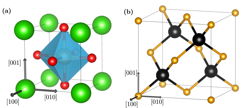
Figure 2: Structures of (a) cubic LiOsO₃ and (b) TiB. Grey arrows indicate the crystallographic directions that form the Cartesian axes.

All our first-principles calculations are carried out with a plane-wave cutoff of 60 Ha, a Gaussian smearing of $0.01$ Ha and the BZ is sampled with a dense Monkhorst-Pack mesh of $20\times 20\times 20$ $\mathbf{k}$ points. The crystal structures are relaxed until all the forces are smaller than $0.5\times 10^{-7}$ Ha/bohr, obtaining a unit cell parameter of $a=9.176$ bohr for TiB and $a=9.879$ bohr for SiP. For LiOsO₃, we obtain a relaxed cell parameter of $a=7.132$ bohr with LDA and $a=7.253$ bohr with GGA.

The active subspace is chosen to be either $M=10$ or $M=14$ for TiB, $M=8$ for SiP and $M=20$ for LiOsO₃. These choices guarantee that the active subspace forms an isolated group of bands in all cases, following the observations in the last paragraph of Sec. III.2. (Using two different values for $M$ in the case of TiB allows us to test the consistency of our implementation, and more specifically the independence of the converged results on the dimension of the active subspace.)

V.2 TiB and SiP

We shall start by testing our implementation with the two simple metals TiB and SiP. The symmetries of the materials substantially reduce the number of independent components of $\boldsymbol{\Phi}^{(1)}$ and $\boldsymbol{\bar{C}}^{\kappa}$. For example, Eq. (68) reduces to $\phi=\lambda$, since [6]

$$\begin{split}\Phi^{(1,\gamma)}_{\kappa\alpha,\kappa^{\prime}\beta}&=(-1)^{\kappa+1}(1-\delta_{\kappa\kappa^{\prime}})\phi\absolutevalue{\epsilon_{\alpha\beta\gamma}},\\ \Lambda^{\kappa}_{\alpha\beta\gamma}&=(-1)^{\kappa+1}\lambda\absolutevalue{\epsilon_{\alpha\beta\gamma}},\end{split}$$ (70)

where $\epsilon_{\alpha\beta\gamma}$ is the Levi-Civita symbol. In Table 1 we show the independent components of the (type-II) flexoelectric force-response tensor, and Table 2 shows the only independent component of $\boldsymbol{\Phi}^{(1)}$ ($\boldsymbol{\Lambda}$), indicated as $\phi$ ($\lambda$). The sum rules Eq. (68) and Eq. (69) are validated to a remarkably high level of accuracy.

Table 1: Linearly independent components of the flexoelectric force-response tensor (in eV) and the clamped-ion elastic tensor (in GPa) for TiB and SiP. The latter is computed via the sublattice sum of $\bar{C}^{\kappa}_{\alpha\gamma,\beta\delta}$ as indicated by Eq. (69), and with the standard HWRV implementation.

		$xx,xx$	$xx,yy$	$xy,xy$
TiB	$\bar{C}^{\text{Ti}}_{\alpha\gamma,\beta\delta}$	5.503	10.373	7.110
	$\bar{C}^{\text{B}}_{\alpha\gamma,\beta\delta}$	10.225	12.163	6.428
	$\bar{C}_{\alpha\gamma,\beta\delta}$	88.108	126.250	75.843
	$\bar{C}^{\text{HWRV}}_{\alpha\gamma,\beta\delta}$	88.069	126.186	75.812
SiP	$\bar{C}^{\text{Si}}_{\alpha\gamma,\beta\delta}$	8.542	14.861	7.034
	$\bar{C}^{\text{P}}_{\alpha\gamma,\beta\delta}$	1.572	7.911	3.676
	$\bar{C}_{\alpha\gamma,\beta\delta}$	45.373	102.162	48.049
	$\bar{C}^{\text{HWRV}}_{\alpha\gamma,\beta\delta}$	45.615	102.223	48.260

Table 2: A comparison between $\phi$ and $\lambda$, in $10^{-3}$ Ha/bohr units (see Eq. 70). $\phi$ is computed with our long-wave ensemble DFPT formalism presented in this work and $\lambda$ with the standard HWRV implementation.

	$\phi$	$\lambda$
TiB	224.360	224.368
SiP	287.126	287.340

As an additional test of our implementation, we show in Fig. 3 the computed $\phi$ parameter for TiB as a function of the $\mathbf{k}$ points mesh resolution. Furthermore, in order to prove that results remain unaltered irrespective of variations in the parameter $M$ (size of the active subspace), we show a comparison between $M=10$ and $M=14$. The obtained results reveal a high level of agreement, which corroborates the robustness of our implementation. (The discrepancies between the results obtained with $M=10$ and $M=14$ in Fig. 3 for small $\mathbf{k}$ points samplings can be attributed to the shift in $\mathbf{k}$ space that we discussed in Sec. III.2. Had we adhered to Eq. (33), instead of utilizing Eq. (45), the results in Fig. 3 would have aligned perfectly, regardless of the number of $\mathbf{k}$ points employed in the calculation.)

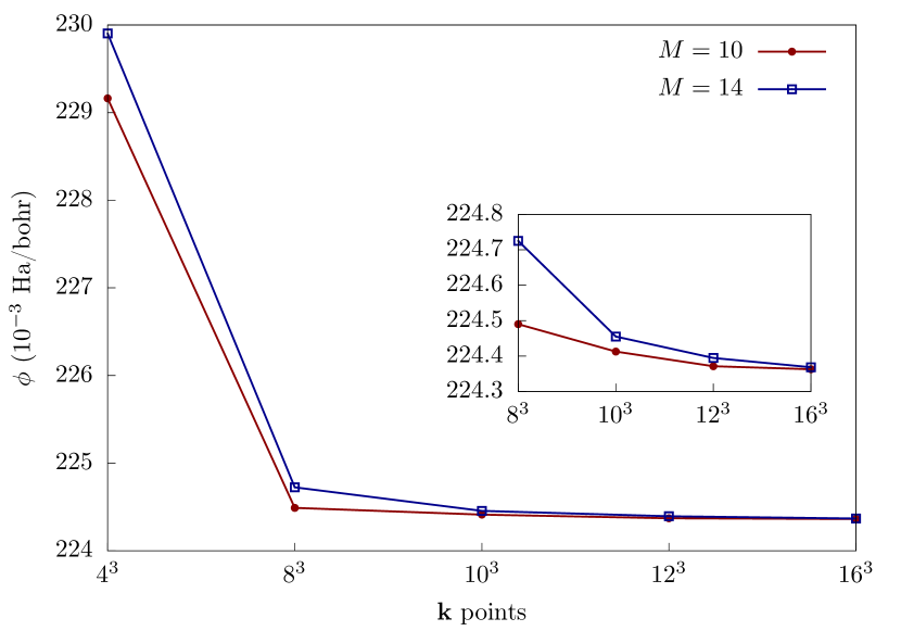
Figure 3: Convergence of the $\phi$ parameter (see Eq. (70)) for TiB as a function of the $\mathbf{k}$ point mesh resolution, for $M=10$ and $M=14$. This is a numerical validation that, as long as the highest states considered in the calculation have vanishing occupations, all the observables that can be extracted from the energy functional are independent of the size of the active subspace, $M$. Solid lines are a guide to the eye.

To conclude with the zincblende structures and in order to validate the sum rules Eq. (68) and (69) in presence of nonvanshing forces and stresses, we apply a displacement of 0.3 bohr along the $x$ Cartesian direction to the B atom in TiB. The resulting crystal structure belongs to the space group $Imm2$ and we obtain, in absolute value, maximum interatomic forces of $3\times 10^{-2}$ Ha$/$bohr and stress components of $3.5\times 10^{-4}$ Ha${}^{3}/$bohr. Table 3 and 4 show selected tensor elements of $\boldsymbol{\Phi}^{(1)}$ and $\boldsymbol{\bar{C}}$, respectively.

Table 3: Independent components of the piezoelectric force-response tensor of distorted TiB, computed with the standard HWRV implementation and with the sum rule of Eq. (68). The prime symbol indicates that the contribution coming from the interatomic forces has not been taken into account. Values are given in $10^{-3}$ Ha/bohr.

	HWRV	[Eq. (68)]′	Eq. (68)
$\Lambda^{\text{Ti}}_{xxx}$	64.420	35.140	64.417
$\Lambda^{\text{Ti}}_{xyy}$	$-$104.004	$-$104.876	$-$104.876
$\Lambda^{\text{Ti}}_{xzy}$	$-$221.380	$-$220.530	$-$220.530
$\Lambda^{\text{Ti}}_{yxy}$	$-$49.769	$-$78.171	$-$48.894
$\Lambda^{\text{Ti}}_{yzx}$	$-$231.073	$-$231.070	$-$231.070

Table 4: Selected clamped-ion elastic tensor coefficients of distorted TiB, computed with the standard HWRV implementation and with the sum rule of Eq. (69). The prime symbol indicates that the contributions coming from the stress have not been taken into account. Values are given in GPa units.

	$\bar{C}^{\text{HWRV}}_{\alpha\gamma,\beta\delta}$	[Eq. (69)]′	Eq. (69)
$xx,xx$	78.258	76.822	78.293
$xx,yy$	122.877	125.366	122.943
$xx,yz$	19.023	29.251	19.038
$xy,xy$	71.972	70.060	72.007
$xy,xz$	17.575	12.478	17.584
$yx,xy$	71.972	73.958	72.011
$yx,xz$	17.575	22.695	17.589
$yy,xx$	122.877	121.470	122.941
$yy,yy$	87.762	90.233	87.810
$yy,yz$	31.655	41.900	31.687
$yy,zz$	135.424	137.935	135.512
$yz,yy$	31.655	21.449	31.662

V.3 Cubic LiOsO₃

In the cubic phase of LiOsO₃ all the atoms sit at inversion centers, resulting in a vanishing $\boldsymbol{\Phi}^{(1)}$ tensor. This system represents, however, the ideal scenario for testing our implementation in the context of strain gradients, as the flexocoupling coefficients of cubic lithium osmate have been previously computed in Ref. [27]. Table 5 presents the calculated independent components for the flexoelectric force-response tensor, along with the numerical validation of Eq. (69). Additionally, the last two rows of Table 5 display the independent components of the flexocoupling tensor, computed by means of Eq. (65). The penultimate row shows the numerical values obtained in the present work, whereas the last row corresponds to the results from Ref. [27].

The agreement between the present results with those of Ref. [27] is remarkable, especially considering the different computational strategy employed therein. (In Ref. [27], the flexocoupling coefficients were calculated via lattice sums of the real-space interatomic FCs, as opposed to the analytical long-wave approach presented here.) Regarding the effect of different schemes for the exchange-correlation functional, we observe that the equilibrium volume slightly differs between LDA and GGA, following the expected trends: we obtain $\Omega=362.756$ bohr³ and $\Omega=381.532$ bohr³, respectively. In general, the calculated values for the flexoelectric force-response tensor and the flexocoupling coefficients show only a small dependence on the choice of the exchange and correlation model. It is also worth mentioning that the limitations of the long-wave module as implemented in the v9 version of abinit prohibits the use of pseudopotentials that include non-linear core corrections. The small disparities for the elastic constants and the flexocoupling tensor obtained with the PBE parametrization of the GGA between Ref. [27] and this work can be largely attributed to the differences in the pseudopotentials.

Atom	$xx,xx$		$xx,yy$		$xy,xy$
	LDA	GGA	LDA	GGA	LDA	GGA
Li	0.95	0.75	10.22	9.99	0.30	0.32
Os	62.97	58.18	24.77	22.67	16.02	15.90
O1	$-$1.08	$-$0.99	$-$2.80	$-$2.44	$-$3.28	$-$3.37
O2	$-$1.08	$-$0.99	9.84	10.13	$-$0.63	$-$0.01
O3	85.00	71.51	6.17	5.07	1.54	2.70
$\bar{C}_{\alpha\gamma,\beta\delta}$	437.42	364.05	143.67	128.73	41.57	44.04
$\bar{C}^{\text{HWRV}}_{\alpha\gamma,\beta\delta}$	437.44	364.19	143.31	128.63	41.83	44.16
Ref. [27]	$\dots$	364.7	$\dots$	129.5	$\dots$	44.3
$f_{\alpha\gamma,\beta\delta}$	$-$14.10	$-$14.24	49.65	47.56	3.69	3.33
Ref. [27]	$\dots$	$-$13.8	$\dots$	49.3	$\dots$	3.3

Table 5: Linearly independent components of the flexoelectric force-response tensor (in eV), the clamped-ion elastic tensor (in GPa) and the flexocoupling tensor (in eV) for cubic LiOsO₃. Values are obtained either with the Perdew-Wang parametrization of the LDA or with the PBE parametrization of the GGA.

VI Conclusions

By combining the virtues of ensemble density-functional theory [28] and density-functional perturbation theory [4], we have established a general and powerful first-principles approach for higher-order derivatives of the total energy in metals. We have focused our numerical tests on the calculation of the flexoelectric coupling coefficients, where our formalism offers drastic improvements, both in terms of accuracy and computational efficiency, compared to earlier approaches. Thereby, our method will greatly facilitate the first-principles-based modeling of polar and ferroelectric metals, which are currently under intense scrutiny within the research community. This work also opens numerous exciting avenues for future work; we shall outline some of them in the following.

First, the advantages of the approach presented here can be immediately extended to other adiabatic spatial dispersion properties via minor modifications to our formulas. For example, by combining the phonon perturbation with a scalar potential one in Eq. (49), our method would yield the “adiabatic Born effective charges” as defined in Ref. [56, 57]. The present approach works directly at the $\Gamma$ point, and hence avoids the need for cumbersome numerical fits. On the other hand, by targeting the adiabatic response to a static (but spatially nonuniform) vector potential field, the present theory could be used to generalize the theory of orbital magnetic susceptibility of Ref. [58] to metals.

Second, note that the scopes of our work go well beyond the specifics of long-wavelength expansions. Our main conceptual achievement consists in generalizing the “$2n+1$” theorem [4], one of the mainstays of DFPT in insulators, to metallic systems. This result opens exciting opportunities for calculating not only spatial dispersion effects, but also nonlinear response properties in metals, with comparable advantages at the formal and practical level. The study of nonlinear optics appears as a particularly attractive topic in this context, although its inherent dynamical nature would require generalizing the formalism presented here to the nonadiabatic regime. We regard this as a promising avenue for future developments of our method.

Appendix A Treatment of the macroscopic electrostatic term in the $\mathbf{q}\rightarrow\mathbf{0}$ limit

A.1 Long-wave limit of external potentials

We shall start by reviewing the long-wavelength behavior of the external potentials, highlighting the differences between insulators and metals.

A.1.1 Insulators

The external potential at first-order in response to an atomic displacement perturbation is usually expressed as a sum of a local plus a separable part [36, 5]. For our scopes, the latter can be omitted, as no divergences associated to the separable part are present in the long-wave limit. The macroscopic component ($\mathbf{G=0}$) of the local part is given by [36]

$$V_{\mathbf{q}}^{\text{loc},\tau_{\kappa\alpha}}(\mathbf{G=0})\sim-i\frac{q_{\alpha}}{\Omega}\left(-\frac{4\pi Z_{\kappa}}{q^{2}}+\frac{F^{\prime\prime}_{\kappa}}{2}\right),$$ (71)

where $F_{\kappa}^{\prime\prime}$ is the second derivative in $q$ of $F_{\kappa}(q)=q^{2}v_{\kappa}^{\text{loc}}(q)$, with $v_{\kappa}^{\text{loc}}(q)\sim-4\pi Z_{\kappa}/q^{2}$, and $Z_{\kappa}$ is the bare nuclear pseudo-charge. The Hartree potential, on the other hand, is given by

$$V_{\mathbf{q}}^{\text{H},\tau_{\kappa\alpha}}=\frac{4\pi}{q^{2}}\rho_{\tau_{\kappa\alpha}}^{\mathbf{q}},$$ (72)

where the lower terms in the Taylor expansion of the first-order electron density (in powers of $\mathbf{q}$) are given by

$$\rho^{\mathbf{q}}_{\tau_{\kappa\alpha}}\sim-iq_{\gamma}\rho^{(1,\gamma)}_{\kappa\alpha}-\frac{q_{\gamma}q_{\delta}}{2}\rho^{(2,\gamma\delta)}_{\kappa\alpha}+\dots$$ (73)

The sum of the local and Hartree potentials then reads as (we omit terms that vanish in the $\mathbf{q}\rightarrow\mathbf{0}$ limit)

$$V_{\mathbf{q}}^{\text{loc}+\text{{H}},\tau_{\kappa\alpha}}\simeq\frac{4\pi}{\Omega}\left(\frac{iq_{\gamma}Z^{(\gamma)}_{\kappa\alpha}}{q^{2}}+\frac{q_{\gamma}q_{\delta}}{2q^{2}}Q^{(\gamma\delta)}_{\kappa\alpha}\right),$$ (74)

where the tensors $Z^{(\gamma)}_{\kappa\alpha}$ and $Q^{(\gamma\delta)}_{\kappa\alpha}$ are, respectively, the screened (short-circuit electrical boundary conditions are assumed) “Born effective charges” and “dynamical quadrupoles”,

$$\begin{split}Z^{(\gamma)}_{\kappa\alpha}&=Z_{\kappa}\delta_{\alpha\gamma}-\Omega\rho^{(1,\gamma)}_{\kappa\alpha},\\ Q^{(\gamma\delta)}_{\kappa\alpha}&=-\Omega\rho^{(2,\gamma\delta)}_{\kappa\alpha}.\end{split}$$ (75)

As a consequence, as long as the “Born effective charges” do not vanish, in an insulator the potential given by Eq. (74) diverges as $\mathcal{O}(q^{-1})$, corresponding to the well-known Frölich term in the scattering potential.

A.1.2 Metals

As we already declared in Sec. III.4, in metals the potential should be an analytic function of the wave vector $\mathbf{q}$, which implies that the divergences that we have encountered in Eq. (74) should disappear. This involves

$$Z^{(\gamma)}_{\kappa\alpha}=0,\quad\Omega\rho^{(1,\gamma)}_{\kappa\alpha}=\delta_{\alpha\gamma}Z_{\kappa}.$$ (76)

In addition, the quadrupoles must be isotropic,

$$Q^{(\gamma\delta)}_{\kappa\alpha}=\delta_{\delta\gamma}Q_{\kappa\alpha}.$$ (77)

We reach the conclusion that in a metal, the first-order electron density in response to an atomic displacement acquires the following form,

$$\Omega\rho^{\mathbf{q}}_{\kappa\alpha}\sim-iq_{\alpha}Z_{\kappa}+\frac{q^{2}}{2}Q_{\kappa\alpha}.$$ (78)

When summing the local and the Hartree potential terms, the divergencies cancel out and, at leading order in $\mathbf{q}$, the scattering potential tends to a direction-independent constant,

$$V_{\mathbf{q}}^{\text{loc+H},\tau_{\kappa\alpha}}\sim\frac{2\pi}{\Omega}Q_{\kappa\alpha},$$ (79)

which is uniquely determined by the charge neutrality of the unit cell and corresponds to the Fermi level shifts defined in Sec. III.4,

$$\frac{2\pi}{\Omega}Q_{\kappa\alpha}=-\mu^{\tau_{\kappa\alpha}}.$$ (80)

A.2 The macroscopic electrostatic energy

A.2.1 Phonons

We want to take the first $\mathbf{q}$ derivative of the three terms that contribute to the macroscopic electrostatic energy in metals, within the framework of variational spatial dispersion theory. To this end, we shall write down the finite $\mathbf{q}$ expressions and we shall take the $\mathbf{q}\rightarrow\mathbf{0}$ limit once the divergencies coming from all the three terms have been properly treated.

The first contribution to the macroscopic electrostatics comes from the ion-ion Ewald (Ew) term,

$$\begin{split}E_{\text{Ew},\mathbf{q}}^{\tau_{\kappa\alpha}\tau_{\kappa^{\prime}\beta}}(\mathbf{G=0})&=Z_{\kappa}Z_{\kappa^{\prime}}\frac{4\pi}{\Omega}\frac{q_{\alpha}q_{\beta}}{q^{2}}e^{-\frac{q^{2}}{4\Lambda^{2}}}\\ &\simeq Z_{\kappa}Z_{\kappa^{\prime}}\frac{4\pi}{\Omega}\left(\frac{q_{\alpha}q_{\beta}}{q^{2}}-\frac{q_{\alpha}q_{\beta}}{4\Lambda^{2}}+\dots\right),\end{split}$$ (81)

where the dots stand for an analytic sum of higher-order terms containing even powers of $\mathbf{q}$. Its partial derivative with respect to the wave vector $q_{\gamma}$ is

$$E_{\text{Ew},\gamma}^{\tau_{\kappa\alpha}\tau_{\kappa^{\prime}\beta}}\simeq\left[\frac{4\pi}{\Omega}\frac{Z_{\kappa}Z_{\kappa^{\prime}}}{q^{2}}\left(\delta_{\alpha\gamma}q_{\beta}+\delta_{\beta\gamma}q_{\alpha}\right)-\frac{8\pi}{\Omega}Z_{\kappa}Z_{\kappa^{\prime}}\frac{q_{\alpha}q_{\beta}q_{\gamma}}{q^{4}}\right]_{\mathbf{q=0}}.$$ (82)

In Eq. (82) and in the following derivations, we omit terms that vanish in the $\mathbf{q=0}$ limit, and we also exclude the $\mathbf{G=0}$ label in order to keep the notation as simple as possible.

The second contribution comes from the second line of Eq. (33), which we shall refer to as the “elst” term, and can be equivalently written in reciprocal space as

$$E_{\text{elst},\mathbf{q}}^{\tau_{\kappa\alpha}\tau_{\kappa^{\prime}\beta}}=\Omega(\rho^{\mathbf{q}}_{\kappa\alpha})^{*}K_{\mathbf{q}}\rho^{\mathbf{q}}_{\kappa^{\prime}\beta},$$ (83)

where $K_{\mathbf{q}}=4\pi/q^{2}$ is the Coulomb kernel. The partial derivative of Eq. (83) with respect to $q_{\gamma}$, within the context of our variational spatial dispersion theory, i.e., excluding the partial $\mathbf{q}$ derivatives of the first-order electron densities, is given by

$$\begin{split}E_{\text{elst},\gamma}^{\tau_{\kappa\alpha}\tau_{\kappa^{\prime}\beta}}&=\left[\Omega(\rho^{\mathbf{q}}_{\tau_{\kappa\alpha}})^{*}K_{\gamma}\rho^{\mathbf{q}}_{\kappa^{\prime}\beta}\right]_{\mathbf{q=0}}\\ &\simeq\frac{1}{\Omega}\left(iq_{\alpha}Z_{\kappa}+\frac{q^{2}}{2}Q_{\kappa\alpha}\right)\left(-\frac{8\pi q_{\gamma}}{q^{4}}\right)\left(-iq_{\beta}Z_{\kappa^{\prime}}+\frac{q^{2}}{2}Q_{\kappa^{\prime}\beta}\right)\bigg{|}_{\mathbf{q=0}}\\ &\simeq\left[-\frac{8\pi}{\Omega}Z_{\kappa}Z_{\kappa^{\prime}}\frac{q_{\alpha}q_{\beta}q_{\gamma}}{q^{4}}+2\left(i\delta_{\alpha\gamma}Z_{\kappa}\mu^{\tau_{\kappa^{\prime}\beta}}-i\delta_{\beta\gamma}\mu^{\tau_{\kappa\alpha}}Z_{\kappa^{\prime}}\right)\right]_{\mathbf{q=0}}.\end{split}$$ (84)

In order to compute the third and last contribution to the macroscopic electrostatic energy, which comes from the local (loc) potentials in the first line of the occupation term, Eq. (52), we need the first $\mathbf{q}$ derivative of the local part of the psuedopotential given in Eq. (71),

$$V_{\gamma}^{\text{loc},\tau_{\kappa\alpha}}\simeq\frac{4\pi i}{\Omega}\left[Z_{\kappa}\frac{\delta_{\alpha\gamma}}{q^{2}}-2Z_{\kappa}\frac{q_{\alpha}q_{\gamma}}{q^{4}}\right]_{\mathbf{q=0}}.$$ (85)

This leads to

$$\begin{split}E_{\text{loc},\gamma}^{\tau_{\kappa\alpha}\tau_{\kappa\beta}}&=\left[\Omega(\rho^{\mathbf{q}}_{\kappa\alpha})^{*}V_{\gamma}^{\text{loc},\tau_{\kappa^{\prime}\beta}}+\Omega(V_{\gamma}^{\text{loc},\tau_{\kappa\alpha}})^{*}\rho^{\mathbf{q}}_{\kappa^{\prime}\beta}\right]_{\mathbf{q=0}}\\ &\simeq\left[\left(iq_{\alpha}Z_{\kappa}+\frac{q^{2}}{2}Q_{\kappa\alpha}\right)\frac{4\pi i}{\Omega}\left(Z_{\kappa^{\prime}}\frac{\delta_{\beta\gamma}}{q^{2}}-2Z_{\kappa^{\prime}}\frac{q_{\beta}q_{\gamma}}{q^{4}}\right)-\frac{4\pi i}{\Omega}\left(Z_{\kappa}\frac{\delta_{\alpha\gamma}}{q^{2}}-2Z_{\kappa}\frac{q_{\alpha}q_{\gamma}}{q^{4}}\right)\left(-iq_{\beta}Z_{\kappa^{\prime}}+\frac{q^{2}}{2}Q_{\kappa^{\prime}\beta}\right)\right]_{\mathbf{q=0}}\\ &\simeq\left[-\frac{4\pi}{\Omega}\frac{Z_{\kappa}Z_{\kappa^{\prime}}}{q^{2}}\left(\delta_{\alpha\gamma}q_{\beta}+\delta_{\beta\gamma}q_{\alpha}\right)+\frac{16\pi}{\Omega}Z_{\kappa}Z_{\kappa^{\prime}}\frac{q_{\alpha}q_{\beta}q_{\gamma}}{q^{4}}+i\delta_{\beta\gamma}\mu^{\tau_{\kappa\alpha}}Z_{\kappa^{\prime}}-i\delta_{\alpha\gamma}Z_{\kappa}\mu^{\tau_{\kappa^{\prime}\beta}}\right]_{\mathbf{q=0}}.\end{split}$$ (86)

When the three contributions are treated together, all the divergences cancel out, and we are left with the following final result,

$$\begin{split}E_{\text{mac},\gamma}^{\tau_{\kappa\alpha}\tau_{\kappa^{\prime}\beta}}&=E_{\text{Ew},\gamma}^{\tau_{\kappa\alpha}\tau_{\kappa^{\prime}\beta}}+E_{\text{elst},\gamma}^{\tau_{\kappa\alpha}\tau_{\kappa^{\prime}\beta}}+E_{\text{loc},\gamma}^{\tau_{\kappa\alpha}\tau_{\kappa^{\prime}\beta}}\\ &\simeq i\delta_{\alpha\gamma}Z_{\kappa}\mu^{\tau_{\kappa^{\prime}\beta}}-i\delta_{\beta\gamma}\mu^{\tau_{\kappa\alpha}}Z_{\kappa^{\prime}},\end{split}$$ (87)

which is Eq. (58) of the main text.

A.2.2 Strain gradients

It is also interesting for our scopes to analyze the contributions coming from the macroscopic electrostatics at second-order in $\mathbf{q}$. By following the same strategy as in Sec. IV.2, second derivatives in $\mathbf{q}$ can be avoided by treating the acoustic phonon perturbation in the comoving frame as a metric-wave perturbation. The final result for the macroscopic electrostatic contribution reads as

$$\begin{split}E_{\text{mac},\gamma}^{\tau_{\kappa\alpha}\eta_{\beta\delta}}&=E_{\text{elst},\gamma}^{\tau_{\kappa\alpha}\eta_{\beta\delta}}+E_{\text{loc},\gamma}^{\tau_{\kappa\alpha}\eta_{\beta\delta}}\\ &\simeq-\delta_{\alpha\gamma}Z_{\kappa}\mu^{\eta_{\beta\delta}},\end{split}$$ (88)

where $\mu^{\eta_{\beta\delta}}$ is the Fermi level shift produced by a uniform strain.

References

- Wei and Chou [1994] S. Wei and M. Y. Chou, Phys. Rev. B 50, 2221 (1994).
- Gonze [1995a] X. Gonze, Phys. Rev. A 52, 1086 (1995a).
- Gonze [1995b] X. Gonze, Phys. Rev. A 52, 1096 (1995b).
- Baroni et al. [2001] S. Baroni, S. de Gironcoli, A. Dal Corso, and P. Giannozzi, Rev. Mod. Phys. 73, 515 (2001).
- Royo and Stengel [2019] M. Royo and M. Stengel, Phys. Rev. X 9, 021050 (2019).
- Royo and Stengel [2022] M. Royo and M. Stengel, Phys. Rev. B 105, 064101 (2022).
- Zabalo and Stengel [2023] A. Zabalo and M. Stengel, Phys. Rev. Lett. 131, 086902 (2023).
- Zabalo et al. [2022] A. Zabalo, C. E. Dreyer, and M. Stengel, Phys. Rev. B 105, 094305 (2022).
- Methfessel and Paxton [1989] M. Methfessel and A. T. Paxton, Phys. Rev. B 40, 3616 (1989).
- de Gironcoli [1995] S. de Gironcoli, Phys. Rev. B 51, 6773 (1995).
- Giustino [2017] F. Giustino, Rev. Mod. Phys. 89, 015003 (2017).
- Kaplan et al. [2023] D. Kaplan, T. Holder, and B. Yan, Nat. Commun. 14, 3053 (2023).
- Hong et al. [2013] S.-Y. Hong, J. I. Dadap, N. Petrone, P.-C. Yeh, J. Hone, and R. M. Osgood, Phys. Rev. X 3, 021014 (2013).
- Wu et al. [2017] L. Wu, S. Patankar, T. Morimoto, N. L. Nair, E. Thewalt, A. Little, J. G. Analytis, J. E. Moore, and J. Orenstein, Nat. Phys. 13, 350 (2017).
- Liu et al. [2023] X. Liu, S. S. Tsirkin, and I. Souza, arXiv preprint arXiv:2303.10129 (2023).
- Zhang et al. [2018] Y. Zhang, Y. Sun, and B. Yan, Phys. Rev. B 97, 041101 (2018).
- Shen [1984] Y.-R. Shen, Principles of nonlinear optics (Wiley-Interscience, New York, NY, USA, 1984).
- Óscar Pozo Ocaña and Souza [2023] Óscar Pozo Ocaña and I. Souza, SciPost Phys. 14, 118 (2023).
- Zhong et al. [2016] S. Zhong, J. E. Moore, and I. Souza, Phys. Rev. Lett. 116, 077201 (2016).
- Malashevich and Souza [2010] A. Malashevich and I. Souza, Phys. Rev. B 82, 245118 (2010).
- Melrose and McPhedran [1991] D. B. Melrose and R. C. McPhedran, Electromagnetic Processes in Dispersive Media (Cambridge University Press, 1991).
- Agranovich and Ginzburg [2013] V. M. Agranovich and V. Ginzburg, Crystal optics with spatial dispersion, and excitons, Vol. 42 (Springer Science & Business Media, 2013).
- Jönsson et al. [1996] L. Jönsson, Z. H. Levine, and J. W. Wilkins, Phys. Rev. Lett. 76, 1372 (1996).
- Dal Corso and Mauri [1994] A. Dal Corso and F. Mauri, Phys. Rev. B 50, 5756 (1994).
- Veithen et al. [2005] M. Veithen, X. Gonze, and P. Ghosez, Phys. Rev. B 71, 125107 (2005).
- Corso et al. [1996] A. D. Corso, F. Mauri, and A. Rubio, Phys. Rev. B 53, 15638 (1996).
- Zabalo and Stengel [2021] A. Zabalo and M. Stengel, Phys. Rev. Lett. 126, 127601 (2021).
- Marzari et al. [1997] N. Marzari, D. Vanderbilt, and M. C. Payne, Phys. Rev. Lett. 79, 1337 (1997).
- Mermin [1965] N. D. Mermin, Phys. Rev. 137, A1441 (1965).
- Marzari et al. [1999] N. Marzari, D. Vanderbilt, A. De Vita, and M. C. Payne, Phys. Rev. Lett. 82, 3296 (1999).
- Gillan [1989] M. J. Gillan, J. Phys.: Condens. Matter 1, 689 (1989).
- Grumbach et al. [1994] M. P. Grumbach, D. Hohl, R. M. Martin, and R. Car, J. Phys.: Condens. Matter 6, 1999 (1994).
- Wentzcovitch et al. [1992] R. M. Wentzcovitch, J. L. Martins, and P. B. Allen, Phys. Rev. B 45, 11372 (1992).
- VandeVondele and De Vita [1999] J. VandeVondele and A. De Vita, Phys. Rev. B 60, 13241 (1999).
- Stengel and De Vita [2000] M. Stengel and A. De Vita, Phys. Rev. B 62, 15283 (2000).
- Gonze [1997] X. Gonze, Phys. Rev. B 55, 10337 (1997).
- Kubo [1957] R. Kubo, J. Phys. Soc. Jpn. 12, 570 (1957).
- Gonze and Lee [1997] X. Gonze and C. Lee, Phys. Rev. B 55, 10355 (1997).
- Born and Huang [1954] M. Born and K. Huang, Dynamical theory of crystal lattices (Clarendon press, 1954).
- Stengel [2013] M. Stengel, Phys. Rev. B 88, 174106 (2013).
- Stengel [2023] M. Stengel, arXiv preprint arXiv:2304.06613 (2023).
- Ishito et al. [2023] K. Ishito, H. Mao, Y. Kousaka, Y. Togawa, S. Iwasaki, T. Zhang, S. Murakami, J.-i. Kishine, and T. Satoh, Nat. Phys. 19, 35 (2023).
- Landau and Lifshitz [1984] L. D. Landau and E. M. Lifshitz, Electrodynamics of continuous media, Landau and Lifshitz course of theoretical physics, vol. 8 (Pergamon Press, 1984).
- Stengel [2016] M. Stengel, Phys. Rev. B 93, 245107 (2016).
- Diéguez and Stengel [2022] O. Diéguez and M. Stengel, Phys. Rev. X 12, 031002 (2022).
- Stengel and Vanderbilt [2018] M. Stengel and D. Vanderbilt, Phys. Rev. B 98, 125133 (2018).
- Schiaffino et al. [2019] A. Schiaffino, C. E. Dreyer, D. Vanderbilt, and M. Stengel, Phys. Rev. B 99, 085107 (2019).
- Hamann et al. [2005] D. R. Hamann, X. Wu, K. M. Rabe, and D. Vanderbilt, Phys. Rev. B 71, 035117 (2005).
- Shi et al. [2013] Y. Shi, Y. Guo, X. Wang, A. J. Princep, D. Khalyavin, P. Manuel, Y. Michiue, A. Sato, K. Tsuda, S. Yu, et al., Nat. Mater. 12, 1024 (2013).
- Gonze et al. [2020] X. Gonze, B. Amadon, G. Antonius, F. Arnardi, L. Baguet, J.-M. Beuken, J. Bieder, F. Bottin, J. Bouchet, E. Bousquet, et al., Comput. Phys. Commun. 248, 107042 (2020).
- Gonze et al. [2009] X. Gonze, B. Amadon, P.-M. Anglade, J.-M. Beuken, F. Bottin, P. Boulanger, F. Bruneval, D. Caliste, R. Caracas, M. Côté, et al., Comput. Phys. Commun. 180, 2582 (2009).
- Perdew and Wang [1992] J. P. Perdew and Y. Wang, Phys. Rev. B 45, 13244 (1992).
- Perdew et al. [1996] J. P. Perdew, K. Burke, and M. Ernzerhof, Phys. Rev. Lett. 77, 3865 (1996).
- VAN [2018] Comput. Phys. Comm. 226, 39 (2018).
- Hamann [2013] D. R. Hamann, Phys. Rev. B 88, 085117 (2013).
- Marchese et al. [2024] G. Marchese, F. Macheda, L. Binci, M. Calandra, P. Barone, and F. Mauri, Nat. Phys. 20, 88 (2024).
- Macheda et al. [2022] F. Macheda, P. Barone, and F. Mauri, Phys. Rev. Lett. 129, 185902 (2022).
- Gonze and Zwanziger [2011] X. Gonze and J. W. Zwanziger, Phys. Rev. B 84, 064445 (2011).