Random walks on Coxeter interchange graphs

Abstract.

A tournament is an orientation of a graph. Vertices are players and edges are games, directed away from the winner. Kannan, Tetali and Vempala and McShine showed that tournaments with given score sequence can be rapidly sampled, via simple random walks on the interchange graphs of Brualdi and Li. These graphs are generated by the cyclically directed triangle, in the sense that traversing an edge corresponds to the reversal of such a triangle in a tournament.

We study Coxeter tournaments on Zaslavsky’s signed graphs. These tournaments involve collaborative and solitaire games, as well as the usual competitive games. The interchange graphs are richer in complexity, as a variety of other generators are involved. We prove rapid mixing by an intricate application of Bubley and Dyer’s method of path coupling, using a delicate re-weighting of the graph metric. Geometric connections with the Coxeter permutahedra introduced by Ardila, Castillo, Eur and Postnikov are discussed.

1. Introduction

A tournament is an orientation of a graph. We think of vertices as players and edges as games, the orientation of which indicates the winner. Tournaments are related to the geometry of the permutahedron $\Pi_{n-1}$, which is a classical polytope in discrete convex geometry. See, e.g., [27, 32, 15].

In [14] we introduced Coxeter tournaments, which are associated with orientations of signed graphs, as in Zaslavsky [31], and the Coxeter permutahedra $\Pi_{\Phi}$, recently introduced by Ardila et al. [2]. Coxeter tournaments involve collaborative and solitaire games, as well as the usual competitive games in graph tournaments.

In this work, we show (see Theorem 3 below) that lazy simple random walks rapidly mix on the sets of Coxeter tournaments with given score sequence, that is, on the fibers of the Coxeter permutahedra $\Pi_{\Phi}$. Informally, this means that the walk is close to uniform in the fiber after a short amount of time, yielding an efficient way to sample from this set of interest.

Many combinatorial properties of these structures remain mysterious. The purpose of this work is to explore the associated Coxeter interchange graphs, which encode their combinatorics, via random walks. These graphs, introduced in [13], generalize the interchange graphs introduced by Brualdi and Li [4]. Rapid mixing in the classical setting was established by Kannan, Tetali and Vempala [11] and McShine [20]. We recover these results as a special case of our general strategy.

Once again, let us emphasize that even the classical interchange graphs appear difficult to describe in general. Indeed, in closing [4], Brualdi and Li state that they are “fascinating combinatorial structures and that much remains to be determined.” For instance, asymptotic estimates for the number of vertices in these graphs are known only for fibers corresponding to points near the center of $\Pi_{n-1}$, by the work of Spencer [26] and McKay et al. [18, 19, 10]. In the other extreme, Chen et al. [7] showed that, for a specific point near the boundary of $\Pi_{n-1}$, the interchange graph is isomorphic to the classical hypercube. The Coxeter interchange graphs are richer still. Therefore, in broad terms, we show that simple random walks rapidly mix on a wide and intricate class of graphs.

This work touches on a variety of subjects (combinatorics, geometry, algebra and probability) and some preliminaries are required before we can state our results precisely. In Section 1.1, we discuss the literature related to tournaments and the standard permutahedron $\Pi_{n-1}$ (of type $A_{n-1}$). Our results are discussed informally in Sections 1.2 and 1.3. Further background on tournaments, root systems, signed graphs and combinatorial geometry is in Section 2 and in the previous works in this series [15, 14, 13]. Our main result is stated formally in Section 3. See Sections 4, 5 and 6 for the proofs.

We hope that this work will serve as an invitation to step into the Coxeter “worlds” (of types $B_{n}$, $C_{n}$ and $D_{n}$). We believe that “Coxeter combinatorics” is fertile ground, where algebraists, combinatorialists, geometers and probabilists can open new lines of fruitful communication. In particular, many problems in discrete probability likely have a Coxeter analogue, waiting to be discovered.

Contents

1. 1 Introduction
   1. 1.1 Context
   2. 1.2 Purpose
   3. 1.3 Discusssion
   4. 1.4 Acknowledgements
2. 2 Background
   1. 2.1 Coxeter tournaments
   2. 2.2 Interchange graphs
   3. 2.3 Path coupling
3. 3 Main result
4. 4 Connectivity
   1. 4.1 Z-frames
   2. 4.2 Decomposing Z-frames
   3. 4.3 Reversing Coxeter tournaments
5. 5 Interchange networks
   1. 5.1 Classifying networks
   2. 5.2 Extended networks
   3. 5.3 Properties of crystals
6. 6 Rapid mixing
   1. 6.1 Coupling in $B_{n}$ and $D_{n}$
   2. 6.2 Coupling in $C_{n}$

1.1. Context

A tournament is an orientation of the complete graph $K_{n}$, encoded as some $T=\{w_{ij}:i>j\}$ with all $w_{ij}\in\{0,1\}$. Each edge $\{i,j\}$ in $K_{n}$ is oriented as $i\to j$ if $w_{ij}=1$ or $i\leftarrow j$ if $w_{ij}=0$. We think of each edge as a game, directed away from the winner. The win sequence

$${\bf w}(T)=\sum_{i>j}[w_{ij}{\bf e}_{i}+(1-w_{ij}){\bf e}_{j}]$$

lists the total number of wins by each player, where ${\bf e}_{i}\in{\mathbb{Z}}^{n}$ are the standard basis vectors. We let ${\bf w}_{n}=(0,1,\ldots,n-1)$ denote the standard win sequence, corresponding to the transitive (acyclic) tournament in which $w_{ij}=1$ for all $i>j$. In a sense, ${\bf w}_{n}$ and its permutations are as “spread out” as possible.

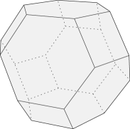
Figure 1. The permutahedron $\Pi_{3}\subset{\mathbb{R}}^{4}$, projected into ${\mathbb{R}}^{3}$. Its 24 vertices correspond to the permutations of the standard win sequence ${\bf w}_{3}=(0,1,2,3)$.

Results by Rado [24] and Landau [16] imply that the set ${\rm Win}(n)$ of all win sequences is precisely the set of lattice points in the permutahedron $\Pi_{n-1}$, that is, ${\rm Win}(n)={\mathbb{Z}}^{n}\cap\Pi_{n-1}$. We recall that $\Pi_{n-1}$ is a classical polytope in discrete geometry (see, e.g., Ziegler [32]), obtained as the convex hull of ${\bf w}_{n}$ and its permutations, see Figure 1. By Stanley [27], win sequences are in bijection with spanning forests $F\subset K_{n}$. (The volume of $\Pi_{n-1}$ is the number of spanning trees $T\subset K_{n}$.) See Postnikov [23] for generalizations.

It is convenient to make a linear shift

$$\Pi_{n-1}^{\prime}=\Pi_{n-1}-\frac{n-1}{2}{\bf 1}_{n},$$ (1)

where ${\bf 1}_{n}=(1,\ldots,1)\in{\mathbb{Z}}^{n}$. Note that this re-centers the polytope at the origin ${\bf 0}_{n}=(0,\ldots,0)\in{\mathbb{Z}}^{n}$. The score sequence

$${\bf s}(T)={\bf w}(T)-\frac{n-1}{2}{\bf 1}_{n},$$

associated with the win sequence ${\bf w}(T)$ of a tournament $T$, is given by

$${\bf s}(T)=\sum_{i>j}(w_{ij}-1/2)({\bf e}_{i}-{\bf e}_{j}).$$ (2)

This shift corresponds to awarding a $\pm 1/2$ point for each win/loss. We let ${\rm Score}(n)$ denote the set of all possible score sequences.

Although the set ${\rm Score}(n)$ has a simple, geometric description, the set ${\rm Tour}(n,{\bf s})$, of tournaments with given score sequence ${\bf s}$, appears to be quite combinatorially complex.

Kannan, Tetali and Vempala [11] investigated simple random walk as a way of sampling from ${\rm Tour}(n,{\bf s})$. However, rapid mixing was proved only for ${\bf s}$ sufficiently close to ${\bf 0}_{n}$. McShine [20] established rapid mixing in time $O(n^{3}\log n)$, for all ${\bf s}\in{\rm Score}(n)$, by an elegant application of Bubley and Dyer’s [5] method of path coupling, which was relatively new at the time. See Section 2.3 below for an overview. We note that Sarkar [25] has shown that mixing takes $\Omega(n^{3})$ for some sequences.

More specifically, in [11, 20], the random walks are on the interchange graphs ${\rm IntGr}(n,{\bf s})$ introduced by Brualdi and Li [4]. Any two tournaments with the same score sequence have the same number of copies of the cyclic triangle $\Delta_{c}$ (see Figure 4). Moreover, if some $T$ contains a copy $\Delta$ of $\Delta_{c}$, then the tournament $T*\Delta$, obtained by reversing the orientation of all edges in $\Delta$, has the same score sequence as $T$. These observations are the key to exploring ${\rm Tour}(n,{\bf s})$. The graph ${\rm IntGr}(n,{\bf s})$ has a vertex $v(T)$ for each $T\in{\rm Tour}(n,{\bf s})$ and two $v(T_{1}),v(T_{2})$ are neighbors if $T_{2}=T_{1}*\Delta$ for some copy $\Delta\subset T_{1}$ of $\Delta_{c}$. It can be shown that ${\rm IntGr}(n,{\bf s})$ is connected. In this sense, $\Delta_{c}$ generates the set ${\rm Tour}(n,{\bf s})$.

The permutahedron $\Pi_{n-1}$ is related with the standard root system of type $A_{n-1}$, as the symmetric group $S_{n}$ is the Weyl group of type $A_{n-1}$. We refer to, e.g., the standard text by Humphreys [9] for background on root systems. We recall that Killing [12] and Cartan [6] classified all (irreducible, crystallographic) root systems (up to isomorphism) as the infinite families $A_{n-1}$, $B_{n}$, $C_{n}$ and $D_{n}$ and the finite exceptional types $E_{6}$, $E_{7}$, $E_{8}$, $F_{4}$ and $G_{2}$.

Coxeter permutahedra $\Pi_{\Phi}$, recently studied by Ardila, Castillo, Eur and Postnikov [2], are obtained by replacing the role of $S_{n}$ in the definition of $\Pi_{n-1}$ with the Weyl group $W_{\Phi}$ of a root system $\Phi$. See, e.g., Figure 2.

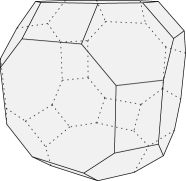
Figure 2. The Coxeter permutahedron of type $C_{3}$.

The previous works in this series [14, 13] studied the connection between the polytopes $\Pi_{\Phi}$ and Coxeter tournaments, which are related to orientations of signed graphs, as developed by Zaslavsky [29, 30, 31]. As mentioned above, these tournaments involve collaborative and solitaire games, as well as the usual competitive games in classical graph tournaments.

1.2. Purpose

In this work (see Theorem 3) we show that simple random walks mix rapidly on the Coxeter interchange graphs ${\rm IntGr}(\Phi,{\bf s})$. These graphs encode the combinatorics of the sets ${\rm Tour}(\Phi,{\bf s})$, of Coxeter tournaments with a given score sequence ${\bf s}$, and give structural information about the fibers of the Coxeter permutahedra $\Pi_{\Phi}$. We focus on the non-standard types $\Phi=B_{n}$, $C_{n}$ and $D_{n}$.

We also show (see Theorem 4) that all Coxeter interchange graphs are connected and we bound their diameter. In constructing our random walk couplings, we uncover various other fine, structural properties of the graphs ${\rm IntGr}(\Phi,{\bf s})$, and hence the sets ${\rm Tour}(\Phi,{\bf s})$, which might be of independent (algebraic, geometric, etc.) interest.

1.3. Discusssion

Path coupling is a powerful method for establishing rapid mixing (see Section 2.3). As already mentioned, path coupling was used in [20]. We will also use this method, however, the application in the Coxeter setting is significantly more delicate.

As discussed above, the interchange graphs in type $A_{n-1}$ are generated by a single neutral tournament, namely, the cyclic triangle $\Delta_{c}$. On the other hand, in the Coxeter setting, there are a number of other generators which play a role (see Figures 5, 6 and 4). A fascinating interplay arises, as these generators can interact in a variety of interesting ways. As such, the Coxeter interchange graphs are much richer in complexity. Likewise, the analysis of random walks on these structures is more involved.

The types increase in difficulty in order $A_{n-1}$, $D_{n}$, $B_{n}$, $C_{n}$. Type $C_{n}$ is especially challenging, due to the presence of loops in some of the generators, which we call clovers (see Figure 6). These generators correspond to double edges in an interchange graph. In particular, a special type of structure, which we call a crystal (see Figure 24), can appear in type $C_{n}$ interchange graphs. See, e.g., Figure 3.

Figure 3. The “snare drum” interchange graph, arising in $C_{3}$, consists of two crystals joined by double edges.

The presence of crystals in type $C_{n}$ interchange graphs leads to two main issues. The first is in extending certain natural, local couplings (on the extended networks discussed in Sections 5.1 and 5.2) to a unified, global coupling. To overcome this difficulty, we will prove a number of detailed combinatorial properties of the Coxeter interchange graphs. We classify the types of local networks (see Figures 13, 16 and 24), which together form the full graph, and study the ways in which they can intersect. For example, one crucial property (see Lemma 20) is that any two crystals can share at most one single edge. Without this property, it seems that a path coupling argument would not be possible.

The second issue caused by crystals is in obtaining a “contractive” (see Section 2.3) coupling. In applying path coupling, we will need to re-weight the graph metric in a specific way, which accounts for the occurrence of crystals. Loosely speaking, the choice of weights is related to the fact that, in our random walk couplings, crystals work like “switches,” that convert single edges to double edges, and vice versa.

The overall coupling used to establish rapid mixing in the Coxeter setting is quite elaborate. See, e.g., Figures 27, 28 and 29 below. The classical type $A_{n-1}$ result [11, 20] is a special case of the argument depicted in Figure 26.

1.4. Acknowledgements

We thank Christina Goldschmidt, James Martin, Sam Olesker-Taylor, Oliver Riordan and Matthias Winkel for helpful conversations. This publication is based on work (MB; RM) partially supported by the EPSRC Centre for Doctoral Training in Mathematics of Random Systems: Analysis, Modelling and Simulation (EP/S023925/1). TP was supported by the Additional Funding Programme for Mathematical Sciences, delivered by EPSRC (EP/V521917/1) and the Heilbronn Institute for Mathematical Research.

2. Background

We refer to Ardila et al. [2], Humphreys [9], Zaslavsky [29, 30, 31], and the previous works in this series [14, 13] for a detailed background on root systems, signed graphs and their connections to discrete geometry. In this section, we will only recall what is used in the current work.

2.1. Coxeter tournaments

A signed graph ${\mathcal{S}}$ on $[n]=\{1,2,\ldots,n\}$ has a set of signed edges $E({\mathcal{S}})$. The four possible types of edges are:

• negative edges $e^{-}_{ij}$ between two vertices $i$ and $j$,

• positive edges $e^{+}_{ij}$ between two vertices $i$ and $j$,

• half edges $e^{h}_{i}$ with only one vertex $i$, and

• loops $e^{\ell}_{i}$ at a vertex $i$.

We note that classical graphs $G$ correspond to signed graphs ${\mathcal{S}}$ with only negative edges.

In this work, we focus on the complete signed graphs ${\mathcal{K}}_{\Phi}$ of types $\Phi=B_{n}$, $C_{n}$ and $D_{n}$. These signed graphs contain all possible negative and positive edges $e_{ij}^{\pm}$. In type $B_{n}$ (resp. $C_{n}$), all possible half edges $e_{i}^{h}$ (resp. loops $e_{i}^{\ell}$) are also included. We call a signed graph ${\mathcal{S}}$ a $\Phi$-graph if ${\mathcal{S}}\subset{\mathcal{K}}_{\Phi}$.

Most of the results in the literature on classical (type $A_{n-1}$) graph tournaments restricts to the case that $G$ is the complete graph $K_{n}$. We note that the signed graph ${\mathcal{K}}_{A_{n-1}}$ with all possible negative edges (and no other types of signed edges) corresponds to the classical complete graph $K_{n}$.

A Coxeter tournament ${\mathcal{T}}$ on a signed graph ${\mathcal{S}}$ is an orientation of ${\mathcal{S}}$. When ${\mathcal{S}}$ is unspecified, our default assumption will be that ${\mathcal{S}}={\mathcal{K}}_{\Phi}$. More formally, ${\mathcal{T}}=\{w_{e}:e\in E({\mathcal{S}})\}$, with all $w_{e}\in\{0,1\}$. We think of each $e\in E({\mathcal{S}})$ as a game, and $w_{e}$ as indicating its outcome.

The score sequence is given by, cf. (2),

$${\bf s}({\mathcal{T}})=\sum_{e\in E({\mathcal{S}})}(w_{e}-1/2){\bf e},$$

where ${\bf e}$ is the vector corresponding to the signed edge $e$, given by ${\bf e}_{ij}^{\pm}={\bf e}_{i}\pm{\bf e}_{j}$, ${\bf e}_{i}^{h}={\bf e}_{i}$ and ${\bf e}_{i}^{\ell}=2{\bf e}_{i}$. In other words:

• negative edges $e_{ij}^{-}$ are competitive games in which one of $i,j$ wins and the other loses a $1/2$ point,

• positive edges $e_{ij}^{+}$ are collaborative games in which $i,j$ both win or lose a $1/2$ point,

• half edges $e_{i}^{h}$ are (half edge) solitaire games in which $i$ wins or loses a $1/2$ point, and

• loops $e_{i}^{\ell}$ are (loop) solitaire games in which $i$ wins or loses $1$ point.

If ${\bf s}({\mathcal{T}})={\bf 0}_{n}$ we say that ${\mathcal{T}}$ is neutral.

We let ${\bf s}_{\Phi}$ denote the standard score sequence corresponding to the Coxeter tournament in which all $w_{e}=1$. We note that, in some contexts, ${\bf s}_{\Phi}$ is called the Weyl vector. It is also the sum of the fundamental weights of the root system $\Phi$. See, e.g., [9, 8] for more details.

As discussed in Ardila et al. [2], the Coxeter $\Phi$-permutahedron $\Pi_{\Phi}$ is the convex hull of the orbit of ${\bf s}_{\Phi}$ under the Weyl group $W_{\Phi}$ of type $\Phi$. Thus ${\bf s}_{\Phi}$ is a distinguished vertex of $\Pi_{\Phi}$. Note that the symmetric group $S_{n}$ is the Weyl group of standard type $\Phi=A_{n-1}$ and the Weyl vector is ${\bf s}_{n}={\bf w}_{n}-\frac{n-1}{2}{\bf 1}_{n}$, so $\Pi_{n-1}^{\prime}$ (see (1) above) is the $\Phi$-permutahedron of standard type $\Phi=A_{n-1}$.

In [14], we showed that $\Pi_{\Phi}$ is precisely the set of all possible mean score sequences of random Coxeter tournaments, thereby establishing a Coxeter analogue of a classical result of Moon [21]. The next work in this series [13] focused on deterministic Coxeter tournaments. The set ${\rm Score}(\Phi)$ of all score sequences of Coxeter tournaments was classified, generalizing the classical result of Landau [16] discussed above.

The precise characterization of ${\rm Score}(\Phi)$ is somewhat technical, involving a certain weak sub-majorization condition and additional parity conditions in types $C_{n}$ and $D_{n}$. The proof is constructive, in that it shows how to build a Coxeter tournament with any given score sequence. See [13, Theorem 4] for more details.

2.2. Interchange graphs

The set ${\rm Tour}(\Phi,{\bf s})$ of all Coxeter tournaments on ${\mathcal{K}}_{\Phi}$ with given score sequence ${\bf s}$ was also investigated in [13]. Coxeter analogues of the interchange graphs ${\rm IntGr}(n,{\bf s})$ discussed above were introduced. Recall that the sets ${\rm Tour}(n,{\bf s})$ are generated by the cyclic triangle $\Delta_{c}$. In the Coxeter setting, there are additional generators.

In all types $B_{n}$, $C_{n}$ and $D_{n}$, in addition to $\Delta_{c}$, we also require a balanced triangle $\Delta_{b}$. In type $B_{n}$, there are also three neutral pairs $\Omega_{1}$, $\Omega_{2}$ and $\Omega_{3}$. On the other hand, in type $C_{n}$, there are also two neutral clovers $\Theta_{1}$ and $\Theta_{2}$. See Figures 4, 5 and 6. In figures depicting Coxeter tournaments, we will draw:

• competitive games as edges directed away from their winner,

• collaborative games as solid/dotted lines if won/lost,

• half edge solitaire games as half edges directed away/toward from their (only) endpoint if won/lost, and

• loop solitaire games as solid/dotted loops if won/lost.

Figure 4. The cyclic and balanced triangles $\Delta_{c}$ and $\Delta_{b}$ are generators in all types $B_{n}$, $C_{n}$ and $D_{n}$.

Figure 5. The neutral pairs $\Omega_{1}$, $\Omega_{2}$ and $\Omega_{3}$ are additional generators in type $B_{n}$.

Figure 6. The neutral clovers $\Theta_{1}$ and $\Theta_{2}$ are additional generators in type $C_{n}$.

The reversal ${\mathcal{T}}^{*}$ of a Coxeter tournament ${\mathcal{T}}=\{w_{e}:e\in E({\mathcal{S}})\}$ on ${\mathcal{S}}$ is obtained by reversing the outcome of all games in ${\mathcal{T}}$. That is, ${\mathcal{T}}^{*}=\{w_{e}^{*}:e\in E({\mathcal{S}})\}$, where $w_{e}^{*}=1-w_{e}$. If ${\mathcal{X}}\subset{\mathcal{T}}$, we let ${\mathcal{T}}*{\mathcal{X}}$ denote the Coxeter tournament obtained from ${\mathcal{T}}$ by reversing the outcome of all games in ${\mathcal{X}}$. In particular, ${\mathcal{T}}^{*}={\mathcal{T}}*{\mathcal{T}}$.

The Coxeter interchange graph ${\rm IntGr}(\Phi,{\bf s})$ has a vertex $v({\mathcal{T}})$ for each ${\mathcal{T}}\in{\rm Tour}(\Phi,{\bf s})$. Vertices $v({\mathcal{T}}_{1}),v({\mathcal{T}}_{2})$ are neighbors if ${\mathcal{T}}_{2}={\mathcal{T}}_{1}*{\mathcal{G}}$, for some copy ${\mathcal{G}}\subset{\mathcal{T}}_{1}$ of a type $\Phi$ generator. If ${\mathcal{G}}$ is a neutral clover, we add a double edge, and otherwise we add a single edge.

For instance, the “snare drum,” in Figure 3 above, is ${\rm IntGr}(C_{3},{\bf s})$ when ${\bf s}=(-1,0,1)$.

The decision to represent clovers as double edges might seem arbitrary at first sight, however, there is a good reason. As it turns out, rather miraculously, this adjustment makes the type $C_{n}$ interchange graphs degree regular. Furthermore, the degree of ${\rm IntGr}(\Phi,{\bf s})$ is related to distances in $\Pi_{\Phi}$ in the following way. Let $\|{\bf x}\|^{2}=\sum_{i}x_{i}^{2}$ denote the squared length of ${\bf x}\in{\mathbb{R}}^{n}$.

Recall that ${\rm Score}(\Phi)$ is the set of all possible score sequences of Coxeter tournaments on ${\mathcal{K}}_{\Phi}$.

Theorem 1 ([13]).

Let $\Phi=B_{n}$, $C_{n}$ or $D_{n}$. Fix any ${\bf s}\in{\rm Score}(\Phi)$. Then the Coxeter interchange graph ${\rm IntGr}(\Phi,{\bf s})$ is regular, with degree given by

$$d(\Phi,{\bf s})=\frac{\|{\bf s}_{\Phi}\|^{2}-\|{\bf s}\|^{2}}{2},$$

where ${\bf s}_{\Phi}$ is the standard score sequence.

In particular, $d(\Phi,{\bf s})=O(n^{3})$.

We observe that, as ${\bf s}$ moves closer to the center ${\bf 0}_{n}$ of the polytope $\Pi_{\Phi}$, the degree $d(\Phi,{\bf s})$ of ${\rm IntGr}(\Phi,{\bf s})$ increases. This is in line with the intuition that Coxeter tournaments with ${\bf s}$ closer to ${\bf 0}_{n}$ (i.e., closer to being neutral) should contain more copies of the (neutral) generators.

In [13], we observed that such a result also holds for graph tournaments, in relation to the standard permutahedron, yielding a geometric interpretation of the classical result (see, e.g., Moon [22]) that any two tournaments with the same win/score sequence have the same number of cyclic triangles.

2.3. Path coupling

We recall that an aperiodic, irreducible discrete-time Markov chain $(X_{n})$ on a finite state space $\Omega$ has a unique equilibrium $\pi$ on $S$ such that, for all $x,y\in\Omega$,

$$p_{n}(x,y)={\mathbb{P}}(X_{n}=y|X_{0}=x)\to\pi(y),$$

as $n\to\infty$. We note that $\pi(y)$ is the asymptotic proportion of time spent at state $y\in\Omega$. The maximal total variation distance from $\pi$ by time $n$,

$$\tau(n)=\max_{x\in\Omega}\frac{1}{2}\sum_{y\in S}|p_{n}(x,y)-\pi(y)|,$$

is non-increasing. The mixing time is defined as

$$t_{\rm mix}=\inf\{n\geqslant 0:\tau(n)\leqslant 1/4\}.$$

A Markov chain is said to be rapidly mixing if $t_{\rm mix}$ is bounded by a polynomial in $\log|\Omega|$.

Path coupling was introduced by Bubley and Dyer [5]. See, e.g., Aldous and Fill [1, Sec. 12.1.12] or Levin et al. [17, Sec. 14.2] for reformulations of the original result that are closer in appearance to that of the following.

Theorem 2 (Path coupling, [5]).

Consider a Markov chain $(X_{n})$ on the vertices of a connected graph $G=(V,E)$. Let $\delta$ denote the graph distance, which assigns weight $\delta(u,v)=1$ to edges $\{u,v\}\in E$. Let $w$ be a re-weighting, assigning some $w(u,v)\geqslant 1$ to $\{u,v\}\in E$. Let $w(x,y)$ be the re-weighted distance between $x,y$ (that is, the minimal total weight of edges along a path between them). Let

$$D_{w}=\max_{x,y\in V}w(x,y)$$

denote the re-weighted diameter of $G$. Suppose that, for some $\alpha>0$, for each $\{x^{\prime},x^{\prime\prime}\}\in E$ there is a coupling $(X_{1}^{\prime},X_{1}^{\prime\prime})$ with $(X_{0}^{\prime},X_{0}^{\prime\prime})=(x^{\prime},x^{\prime\prime})$ so that

$${\mathbb{E}}[w(X_{1}^{\prime},X_{1}^{\prime\prime})]\leqslant(1-\alpha)w(x^{\prime},x^{\prime\prime}).$$

Then $(X_{n})$ mixes in time $t_{\rm mix}=O(\alpha^{-1}\log D_{w})$.

Often this result is applied with $w=\delta$, and, indeed, this will suffice for us in types $B_{n}$ and $D_{n}$. On the other hand, in the more complicated type $C_{n}$, we will select a careful re-weighting $w$ that takes into account some of the delicate, local features of the interchange graphs of this type.

3. Main result

Our main result shows that random walks rapidly mix on the Coxeter interchange graphs.

Theorem 3.

Let $\Phi=B_{n}$, $C_{n}$ or $D_{n}$. Fix any ${\bf s}\in{\rm Score}(\Phi)$. Then lazy simple random walk $({\mathcal{T}}_{n}:n\geqslant 0)$ on ${\rm IntGr}(\Phi,{\bf s})$ mixes in time $t_{\rm mix}=O(n^{3}\log n)$ if $\Phi=B_{n}$ or $D_{n}$, and in time $t_{\rm mix}=O(n^{4}\log n)$ if $\Phi=C_{n}$.

Rapid mixing in type $A_{n-1}$, proved in [11, 20], follows as a special case of our proof of this result in type $D_{n}$.

We note that the classification of ${\rm Score}(\Phi)$ in [14] is constructive, which allows us to initialize the random walk in the first place.

In fact, we will prove sharper bounds (see Theorems 22 and 23 below). In types $B_{n}$ and $D_{n}$, we will show that $t_{\rm mix}=O(d\log n)$, where $d$ is the degree (see Theorem 1 above) of the interchange graph ${\rm IntGr}(\Phi,{\bf s})$. The result above follows, since $d=O(n^{3})$. In type $C_{n}$, we will show that $t_{\rm mix}=O(\gamma d\log n)$, where $\gamma$ is a certain quantity (see Lemma 21) satisfying $\gamma\leqslant\min\{d,2n\}$. We call $\gamma$ the maximal crystal degree of the interchange graph. Roughly speaking, it is maximal number of crystals, all containing the same double edge. This quantity is related to the re-weighting $w$ that we will use in applying Theorem 2 in type $C_{n}$. We note that re-weighting arguments have been used before, e.g., in the work of Wilson [28].

4. Connectivity

Before proving Theorem 3, we will first establish the following combinatorial result, giving further structural information (beyond its regularity, given by Theorem 1) about the Coxeter interchange graphs.

Theorem 4.

Let $\Phi=B_{n}$, $C_{n}$ or $D_{n}$. Fix any ${\bf s}\in{\rm Score}(\Phi$). The Coxeter interchange graph ${\rm IntGr}(\Phi,{\bf s})$ is connected and its diameter $D=O(n^{2})$.

This result is a corollary of Lemma 12 (the “reversing lemma”) proved at the end of this section. A number of preliminaries are required. First, in the next subsection, we will find a way of encoding Coxeter tournaments as special types of directed graphs.

4.1. Z-frames

Oriented signed graphs were studied by Zaslavsky [31]. From this point of view (see [31, Fig. 1]), each oriented signed edge in an oriented signed graph ${\mathcal{S}}$ is the union of at most two directed half edges. We modify this idea, by adding a named endpoint to each half-edge, which we call a match. This will allow us to prove certain structural facts using graph theory techniques. We call such a structure a Z-frame.

Definition 5.

A Z-frame ${\bf Z}$ is a directed, bipartite multigraph on disjoint sets of players $V$ and matches $M$, such that every match has degree $1$ or $2$.

This concept is fairly general, and not all Z-frames correspond to a Coxeter tournament ${\mathcal{T}}$ on some ${\mathcal{S}}\subset{\mathcal{K}}_{\Phi}$. However, each such ${\mathcal{T}}$ has a unique representation as a Z-frame ${\bf Z}({\mathcal{T}})$. We think of ${\bf Z}({\mathcal{T}})$ as revealing the “inner directed graph structure” of ${\mathcal{T}}$. Players in ${\bf Z}({\mathcal{T}})$ correspond to vertices in ${\mathcal{T}}$. Recall that each game in ${\mathcal{T}}$ corresponds to an oriented signed edge. Each such game is associated with a match in ${\bf Z}({\mathcal{T}})$.

We will think of edges directed away/toward players $v\in V$ as positively/negatively charged. We say that $\bf Z$ is neutral if all players $v\in V$ have net zero charge, i.e., ${\rm deg}^{+}(v)-{\rm deg}^{-}(v)=0$, where ${\rm deg}^{\pm}(v)$ is the number of positive/negative edges incident to $v$.

Definition 6.

Let ${\mathcal{T}}$ be a Coxeter tournament on a signed graph ${\mathcal{S}}$ on $[n]$. Let ${\bf Z}({\mathcal{T}})$ be the Z-frame on $V=[n]$ and $M=\{m_{e}\colon e\in{\mathcal{S}}\}$, with the following directed edges:

• If a competitive game $e_{ij}^{-}\in{\mathcal{S}}$ between players $i$ and $j$ is won (resp. lost) by $i$ in ${\mathcal{T}}$, we include two directed edges $i\rightarrow m_{ij}^{-}\rightarrow j$ (resp. $i\leftarrow m_{ij}^{-}\leftarrow j$).

• If a collaborative game $e_{ij}^{+}\in{\mathcal{S}}$ between players $i$ and $j$ is won (resp. lost) in ${\mathcal{T}}$, we include two directed edges $i\rightarrow m_{ij}^{+}\leftarrow j$ (resp. $i\leftarrow m_{ij}^{+}\rightarrow j$).

• If a half edge solitaire game $e_{i}^{h}\in{\mathcal{S}}$ by player $i$ is won (resp. lost) in ${\mathcal{T}}$, we include one directed edge $i\rightarrow m_{i}^{h}$ (resp. $i\leftarrow m_{i}^{h}$).

• If a loop solitaire game $e_{i}^{\ell}\in{\mathcal{S}}$ by player $i$ is won (resp. lost) in ${\mathcal{T}}$, we include two directed edges $i\rightrightarrows m_{i}^{\ell}$ (resp. $i\leftleftarrows m_{i}^{\ell}$).

See Figure 7 for an example of a Coxeter tournament ${\mathcal{T}}$ and its corresponding Z-frame ${\bf Z}({\mathcal{T}})$.

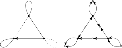
Figure 7. A $C_{3}$-tournament ${\mathcal{T}}$ and its Z-frame ${\bf Z}({\mathcal{T}})$. Players/matches are drawn as black/white dots.

The reason for the above terminology is that directed edges in ${\bf Z}({\mathcal{T}})$ with a positive/negative charge correspond to positive/negative contributions to the score sequence ${\bf s}({\mathcal{T}})$. Note that, in competitive/collaborative games, the two charges are opposing/aligned (regardless of the outcome of the game). See Table 1.

Table 1. Signed edges $e$ in a signed graph ${\mathcal{S}}$ can be oriented in one of two ways $w_{e}\in\{0,1\}$ by a Coxeter tournament ${\mathcal{T}}$. The contribution to the score sequence ${\bf s}({\mathcal{T}})$ and representation in the Z-frame ${\bf Z}({\mathcal{T}})$ are given below.

$e$	$w_{e}$	${\bf s}$	${\bf Z}$
$e_{ij}^{-}$	1	$+{\bf e}_{ij}^{-}/2=+{\bf e}_{i}/2-{\bf e}_{j}/2$	$i\rightarrow m_{ij}^{-}\rightarrow j$
	0	$-{\bf e}_{ij}^{-}/2=-{\bf e}_{i}/2+{\bf e}_{j}/2$	$i\leftarrow m_{ij}^{-}\leftarrow j$
$e_{ij}^{+}$	1	$+{\bf e}_{ij}^{+}/2=+{\bf e}_{i}/2+{\bf e}_{j}/2$	$i\rightarrow m_{ij}^{+}\leftarrow j$
	0	$-{\bf e}_{ij}^{+}/2=-{\bf e}_{i}/2-{\bf e}_{j}/2$	$i\leftarrow m_{ij}^{+}\rightarrow j$
$e_{i}^{h}$	1	$+{\bf e}^{h}_{i}/2=+{\bf e}_{i}/2$	$i\rightarrow m_{i}^{h}$
	0	$-{\bf e}^{h}_{i}/2=-{\bf e}_{i}/2$	$i\leftarrow m_{i}^{h}$
$e_{i}^{\ell}$	1	$+{\bf e}^{\ell}_{i}/2=+{\bf e}_{i}$	$i\rightrightarrows m_{i}^{\ell}$
	0	$-{\bf e}^{\ell}_{i}/2=-{\bf e}_{i}$	$i\leftleftarrows m_{i}^{\ell}$

4.2. Decomposing Z-frames

Our aim is to decompose neutral Coxeter tournaments into irreducible neutral parts. In this section, we will do this for Z-frames in general.

Definition 7.

We call a trail ${\bf T}$ of (directed) edges in a Z-frame closed if it starts and ends at the same vertex, and otherwise we call it open. A trail is neutral if the two consecutive edges at each player $v\in V$ have opposite charges. The length $\ell$ of a trail is its number of matches.

Note that the edges along a trail in a $Z$-frame do not repeat, and are connected to each other in alternation by a player/match. Also note that neutral open trails start and end at distinct final matches (the left and rightmost matches along the trail). See Figure 8.

Figure 8. An open neutral trail of length $\ell=4$.

Lemma 8.

Any neutral Z-frame ${\bf Z}$ can be decomposed into an edge-disjoint union ${\bf Z}=\bigcup_{i}{\bf T}_{i}$ of closed neutral trails and open neutral trails, such that no two open trails have a common final match.

Proof.

Let $v\in V$. Since Z is neutral, ${\rm deg}_{+}(v)={\rm deg}_{-}(v)$. Therefore we may pair each edge directed away from $v$ with an edge directed toward $v$. Note that any such pair is a neutral trail. We let ${\mathcal{P}}_{v}$ denote the set of all such pairs. Then $\bigcup_{v\in V}{\mathcal{P}}_{v}$ is a decomposition of ${\bf Z}$ into an edge-disjoint union of neutral trails. Select a decomposition ${\bf Z}=\bigcup_{i}{\bf T}_{i}$ with the minimal number of neutral trails. Open trails in this decomposition cannot have a common final match, as otherwise they could be concatenated to form a single longer trail, contradicting minimality. ∎

Let ${\bf Z}$ be a neutral Z-frame. We say that ${\bf Z}$ is reducible if it contains a non-empty neutral ${\bf Z}^{\prime}\subsetneq{\bf Z}$. Otherwise, ${\bf Z}$ is irreducible.

Lemma 9.

Let ${\bf Z}$ be an irreducible neutral Z-frame. Then ${\bf Z}$ is a neutral trail and $\mathrm{deg}(v)\in\{0,2,4\}$ for all $v\in V$.

Proof.

By Lemma 8, ${\bf Z}$ is a neutral trail, and so all $\mathrm{deg}(v)$ are even. If $v$ is an isolated vertex that plays no solitaire games, then $\mathrm{deg}(v)=0$. Otherwise, if ${\bf Z}$ is non-trivial, we will argue that $\mathrm{deg}(v)\in\{2,4\}$ are the only possibilities. To see this, start at any $v$ along the trial, and then follow the trail. Consider the charges of the edges incident to $v$, in the order in which they are visited by the trail. If the first and second charges are opposing, then the trail is complete with $\mathrm{deg}(v)=2$. Otherwise, suppose they are both positive (the other case is symmetric). Since ${\bf Z}$ is neutral, the 3rd charge is negative. Finally, consider the 4th charge. If it were positive, then the sub-trail between the third negative edge incident to $v$ and the forth positive edge incident to $v$ would be neutral. Therefore, the 4th charge is negative, and so the trail is complete with $\mathrm{deg}(v)=4$. ∎

4.3. Reversing Coxeter tournaments

Applying the results of the previous section, we obtain the following result for Z-frames ${\bf Z}({\mathcal{T}})$ of Coxeter tournaments ${\mathcal{T}}$.

Lemma 10.

Let $\Phi=B_{n}$, $C_{n}$ or $D_{n}$. Let ${\bf Z}({\mathcal{T}})$ be the Z-frame of a neutral Coxeter tournament ${\mathcal{T}}$ on a signed $\Phi$-graph ${\mathcal{S}}\subset{\mathcal{K}}_{\Phi}$. Consider a decomposition ${\bf Z}({\mathcal{T}})=\bigcup_{i}{\bf T}_{i}$ into neutral trails given by Lemma 8. If $\Phi=C_{n}$ or $D_{n}$ then all trails ${\bf T}_{i}$ are closed. If $\Phi=B_{n}$ then possibly some ${\bf T}_{i}$ are open.

Proof.

This result follows by noting that if ${\mathcal{T}}$ is of type $C_{n}$ or $D_{n}$ then all matches in ${\bf Z}({\mathcal{T}})$ are degree 2. Therefore, there are no open neutral trails in the decomposition, so each ${\bf T}_{i}$ is closed. On the other hand, in type $B_{n}$ it is possible to have open and closed trails, since in this case possibly some matches are degree 1. ∎

Note that a tournament ${\mathcal{T}}$ on a signed graph ${\mathcal{S}}$ is neutral if and only if its Z-frame ${\bf Z}({\mathcal{T}})$ is neutral. Naturally, we call such a ${\mathcal{T}}$ irreducible if ${\bf Z}({\mathcal{T}})$ is irreducible, and reducible otherwise.

Lemma 11.

Suppose that ${\mathcal{S}}$ is a $D_{n}$-graph in which all players $v\in V$ have degree four. Then any neutral tournament ${\mathcal{T}}$ on ${\mathcal{S}}$ is reducible.

Proof.

The proof is by contradiction. Suppose that ${\mathcal{T}}$ on ${\mathcal{S}}$ is neutral and that ${\bf Z}({\mathcal{T}})$ is irreducible. By Lemma 8, ${\bf Z}({\mathcal{T}})$ is in fact a single neutral trail, which for convenience we will denote by $\bf T$. Following the consecutive edges of $\bf T$, we can find a closed trail ${\bf T}^{\prime}\subset{\bf T}$ which:

• starts and ends at some player $v$,

• visits no player $u\neq v$ more than once along the way,

• and is neutral everywhere except at $v$.

Let us assume that the two directed edges in ${\bf T}^{\prime}$ incident to $v$ are positive, since the other case is symmetric.

Consider the extension ${\bf T}^{\prime}\cup{\bf T}^{\prime\prime}$ of ${\bf T}^{\prime}$, as it departs $v$ via some negatively charged directed edge, until it eventually returns to some player $u\in{\bf T}^{\prime}$ for the first time. Note that $u\neq v$, as else, since ${\bf T}$ is irreducible, it would follow that ${\bf T}={\bf T}^{\prime}\cup{\bf T}^{\prime\prime}$, and then that there are degree 2 vertices in ${\bf T}$ along ${\bf T}^{\prime}$. Since ${\bf T}^{\prime}$ is neutral at $u$, the edges in ${\bf T}^{\prime}$ incident to $u$ have opposing charges. Let ${\bf T}^{\prime}={\bf T}^{\prime}_{+}\cup{\bf T}^{\prime}_{-}$, where ${\bf T}^{\prime}_{\pm}\subset{\bf T}^{\prime}$ is the trail between $u$ and $v$ which includes the positive/negative edge in ${\bf T}^{\prime}$ incident to $u$, as in Figure 9. To conclude, consider the charge of the directed edge in ${\bf T}^{\prime\prime}$ along which $u$ is revisited. To obtain the required contradiction, note that if this charge is positive (resp. negative) then ${\bf T}^{\prime}_{-}\cup{\bf T}^{\prime\prime}$ (resp. ${\bf T}^{\prime}_{+}\cup{\bf T}^{\prime\prime}$) is a neutral trail. ∎

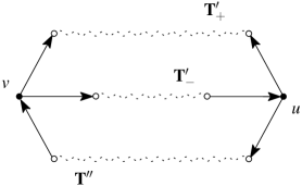
Figure 9. In this instance, the directed edge in ${\bf T}^{\prime\prime}$ along which $u$ is revisited is positive, so ${\bf T}^{\prime}_{-}\cup{\bf T}^{\prime\prime}$ is a neutral trail. If it were negative, then ${\bf T}^{\prime}_{+}\cup{\bf T}^{\prime\prime}$ would be neutral. Curved dotted lines represent the continuation of a trail.

Finally, we turn our attention to the main result of this section.

Lemma 12 (Reversing lemma).

Let $\Phi=B_{n}$, $C_{n}$ or $D_{n}$. Let ${\mathcal{T}}$ be a tournament on the complete signed graph ${\mathcal{K}}_{\Phi}$, and let ${\mathcal{I}}\subset{\mathcal{T}}$ be a neutral sub-tournament. If ${\mathcal{I}}$ has $\ell\geqslant 3$ games then ${\mathcal{I}}$ can be reversed in a series of at most $\ell-2$ type $\Phi$ generator reversals.

The assumption that ${\mathcal{T}}$ is on ${\mathcal{K}}_{\Phi}$ is crucial, since not all of the games in the generators used to reverse ${\mathcal{I}}$ will be in ${\mathcal{I}}$ itself. However, after the series of reversals, only the games in ${\mathcal{I}}$ will have been reoriented, i.e., all games in ${\mathcal{T}}\setminus{\mathcal{I}}$ will be restored to their initial orientations.

Proof.

Without loss of generality we may assume that ${\mathcal{I}}$ is irreducible. In this case, by Lemma 8, the Z-frame ${\mathbf{Z}}({\mathcal{I}})$ is a single neutral trail. For simplicity, we will speak of ${\mathcal{I}}$ as a tournament and trail interchangeably.

We first address the simplest case of open neutral trails, which appears only in type $B_{n}$. We proceed by induction on the length $\ell$. The smallest open trails, with $\ell=3$, are the neutral pairs $\Omega_{i}$ (as in Figure 5) themselves, which are clearly reversible in a single reversal. For longer open neutral trails ${\mathcal{I}}$, consider any (half edge) solitaire game $h$ in ${\mathcal{T}}$ played by some $u$ in ${\mathcal{I}}$, which is not an endpoint of the trail. Using $h$, we can first reverse either the part of the trail that is to the “left” of $u$ or else the part which is to the “right.” We can do this using the inductive hypothesis, as one of the parts is neutral and both have length smaller than $\ell$. Then, using the reversal of this game $h^{*}$, we can reverse the other part of the trail in turn. See Figure 10 for an example.

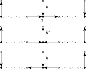
Figure 10. In type $B_{n}$: Reversing an open neutral trail of length $\ell>3$, using a (half edge) solitaire game $h$ played by some $u$ in the “middle” of the trail. In this example, from top to bottom, we first reverse the “right” side of ${\mathcal{I}}$ using $h$, and then the “left” side using $h^{*}$.

Next, we turn to the case of closed neutral trails. Recall that closed trails do not have solitaire half edge games, so from this point on we assume that $\Phi=C_{n}$ or $D_{n}$. If ${\mathcal{I}}$ is generator, then the result clearly holds. If it is not, then let $k\geqslant 3$ be the number of vertices in ${\mathcal{I}}$. If $k=3$, one can verify directly that the result holds. See Figure 11.

Figure 11. Up to symmetry, it suffices to consider the above neutral tournaments on three vertices. Note that each of these tournaments with $\ell$ games can be reversed in $\ell-2$ steps.

For $k\geqslant 4$, we aim to find a pair of vertices $i$, $j$ in ${\mathcal{I}}$ which do not play a game with each other in ${\mathcal{I}}$. Once we find such a pair, the argument is similar to the case of open trails above; the difference being that, in the case of closed trails, we will either first reverse the “top/bottom” (instead of the “left/right”) of the trail, and then the other side in turn, as in Figure 12.

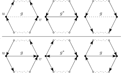
Figure 12. Reversing ${\mathcal{I}}$ when its Z-frame is a closed neutral trail. Above: If the charges of the edges incident to $u$ and $v$ are “aligned,” we use the collaborative game $g$ between $u,v$ to reverse ${\mathcal{I}}$. Below: Otherwise, if they are “unaligned,” we use the competitive game between $u$ and $v$.

To this end, suppose that every pair of vertices in ${\mathcal{I}}$ plays at least one game with each other. As $k\geqslant 4$, this implies that the degree of every player in ${\mathcal{I}}$ is at least $3$. Moreover, if some $v$ in ${\mathcal{I}}$ plays a loop game, then $\deg(v)\geqslant 5$. However, as ${\mathcal{I}}$ is neutral and irreducible, this would contradict Lemma 9. Thus, ${\mathcal{I}}$ is a $4$-regular $D_{n}$-graph. But this is also impossible, by Lemma 11. Therefore, for all $k\geqslant 4$, there exists a pair $i,j$ of players which do not play a game with each other, and this concludes the proof. ∎

Finally, using the reversing lemma, we will prove the main result of this section.

Proof of Theorem 4.

Let ${\mathcal{T}},{\mathcal{T}}^{\prime}\in{\rm Tour}(\Phi,{\bf s})$. The distance between ${\mathcal{T}}$ and ${\mathcal{T}}^{\prime}$ is the smallest number of the generator reversals which transforms ${\mathcal{T}}$ into ${\mathcal{T}}^{\prime}$. The games in the difference ${\mathcal{D}}={\mathcal{T}}\setminus{\mathcal{T}}^{\prime}$ are precisely those which need to be reversed. Since ${\bf s}({\mathcal{T}})={\bf s}({\mathcal{T}}^{\prime})$, it follows that ${\mathcal{D}}$ is neutral. Therefore, by Lemma 12, there is a path from $v({\mathcal{T}})$ to $v({\mathcal{T}}^{\prime})$ in ${\rm IntGr}(\Phi,{\bf s})$ of length $O(n^{2})$. Hence ${\rm IntGr}(\Phi,{\bf s})$ is connected and its diameter $D=O(n^{2})$. ∎

5. Interchange networks

In this section, for ease of exposition, we will speak of Coxeter tournaments ${\mathcal{T}}$ and their corresponding vertices $v({\mathcal{T}})$ in ${\rm IntGr}$ interchangeably.

Definition 13.

For ${\mathcal{T}}_{1},{\mathcal{T}}_{2}\in{\rm Tour}(\Phi,{\bf s})$ at distance two in ${\rm IntGr}(\Phi,{\bf s})$, we define the interchange network $N({\mathcal{T}}_{1},{\mathcal{T}}_{2})$ to be the union over all paths of length two between ${\mathcal{T}}_{1},{\mathcal{T}}_{2}$.

Note that each path of length two between such ${\mathcal{T}}_{1},{\mathcal{T}}_{2}$ corresponds to a way of reversing the difference ${\mathcal{D}}={\mathcal{T}}_{1}\setminus{\mathcal{T}}_{2}$ between ${\mathcal{T}}_{1}$ and ${\mathcal{T}}_{2}$.

5.1. Classifying networks

In this section, we will classify the possibilities for $(N,{\mathcal{D}})$. As we will see, this is the key to applying path coupling (Theorem 2 above) in Section 6 below. In the classical case of type $A_{n-1}$ there is only one possibility for $N$ (a “single diamond”), and this is the reason why such a simple contractive coupling (as in Figure 26 below) is possible. As it turns out, this continues to hold in types $B_{n}$ and $D_{n}$, but the underlying reasons are more complicated. Type $C_{n}$, on the other hand, is significantly more complex, as then the structure of $N$ can take various other forms.

It can be seen that any two distinct generators ${\mathcal{G}}_{1}\neq{\mathcal{G}}_{2}$ are either disjoint ${\mathcal{G}}_{1}\cap{\mathcal{G}}_{2}=\emptyset$ or else have exactly one game $g$ in common ${\mathcal{G}}_{1}\cap{\mathcal{G}}_{2}=\{g\}$. In this case, we say that ${\mathcal{G}}_{1},{\mathcal{G}}_{2}$ are adjacent.

Note that if a path of length two from ${\mathcal{T}}_{1}$ to ${\mathcal{T}}_{2}$ passes through some ${\mathcal{T}}_{12}$, then there are two generators ${\mathcal{G}}_{1},{\mathcal{G}}_{2}\subset{\mathcal{T}}_{12}$ such that ${\mathcal{T}}_{i}={\mathcal{T}}_{12}*{\mathcal{G}}_{i}$, for $i\in\{1,2\}$. In this way, every such path of length two from ${\mathcal{T}}_{1}$ to ${\mathcal{T}}_{2}$ is determined by a midpoint ${\mathcal{T}}_{12}$ and a pair of generators ${\mathcal{G}}_{1},{\mathcal{G}}_{2}\subset{\mathcal{T}}_{12}$.

There are three possible networks when ${\mathcal{G}}_{1},{\mathcal{G}}_{2}$ are disjoint. We call these the single, double and quadruple diamonds. See Figure 13. Recall that double edges in ${\rm IntGr}$ correspond to neutral clover reversals. All other types of reversals (neutral triangles and pairs) are represented as single edges.

Figure 13. Left to right: The single, double and quadruple diamond interchange networks.

The following result classifies the types of networks $N({\mathcal{T}}_{1},{\mathcal{T}}_{2})$ when ${\mathcal{G}}_{1},{\mathcal{G}}_{2}$ are disjoint.

Lemma 14.

Suppose that there is a path of length two between ${\mathcal{T}}_{1},{\mathcal{T}}_{2}$ in ${\rm IntGr}(\Phi,{\bf s})$ that passes through midpoint ${\mathcal{T}}_{12}$, with associated generators ${\mathcal{G}}_{i}\subset{\mathcal{T}}_{12}$ such that ${\mathcal{T}}_{i}={\mathcal{T}}_{12}*{\mathcal{G}}_{i}$. Suppose that ${\mathcal{G}}_{1},{\mathcal{G}}_{2}$ are disjoint. Then if exactly zero, one or two of the ${\mathcal{G}}_{i}$ are clovers then the network $N({\mathcal{T}}_{1},{\mathcal{T}}_{2})$ is a single, double or quadruple diamond, respectively.

Proof.

Clearly, there are exactly two paths from ${\mathcal{T}}_{1}$ to ${\mathcal{T}}_{2}$. These paths correspond to reversing the disjoint generators ${\mathcal{G}}_{1}^{*},{\mathcal{G}}_{2}\subset{\mathcal{T}}_{1}$ in series, in one of the two possible orders. See Figure 14. ∎

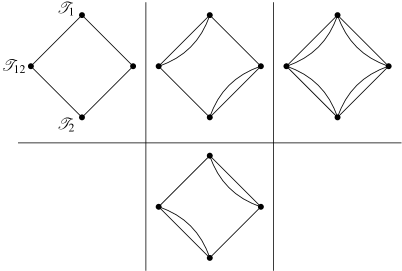
Figure 14. Left to right: $N({\mathcal{T}}_{1},{\mathcal{T}}_{2})$ when exactly zero, one or two of the disjoint ${\mathcal{G}}_{1},{\mathcal{G}}_{2}$ is a clover (single, double and quadruple diamonds). In each cell, the leftmost vertices are ${\mathcal{T}}_{1}$, ${\mathcal{T}}_{12}$ and ${\mathcal{T}}_{2}$, as in the first cell.

The case that ${\mathcal{G}}_{1},{\mathcal{G}}_{2}$ are adjacent is more involved. It is useful to note that, in this case, the difference ${\mathcal{D}}={\mathcal{T}}_{1}\setminus{\mathcal{T}}_{2}$ is a neutral tournament with exactly four games on either three or four vertices. Even so, there are a number of cases to consider, and the key to a concise argument is grouping symmetric cases together. For a Coxeter tournament ${\mathcal{T}}$, we define its projection graph $\pi({\mathcal{T}})$ to be the graph obtained by changing each:

• oriented negative/positive edge (i.e., competitive/collaborative game) into an undirected edge,

• oriented half edge (i.e., half edge solitaire game) into an undirected half edge,

• oriented loop (i.e., loop solitaire game) into an undirected loop.

There are a number of ways that two generators ${\mathcal{G}}_{1},{\mathcal{G}}_{2}$ can be adjacent. However, there are only four possibilities for their projected difference $\pi({\mathcal{D}})$. We call these the square, tent, fork and hanger, as in Figure 15. The following observation is essentially self-evident, and can be verified by an elementary case analysis. We omit the proof.

Figure 15. Left to right: The square, tent, fork, and hanger.

Lemma 15.

Assume the same set up as Lemma 14, except that instead ${\mathcal{G}}_{1},{\mathcal{G}}_{2}$ are adjacent. Let ${\mathcal{D}}={\mathcal{T}}_{1}\setminus{\mathcal{T}}_{2}$. Then:

1. If ${\mathcal{G}}_{1},{\mathcal{G}}_{2}$ are neutral triangles on four/three vertices then $\pi({\mathcal{D}})$ is a square/tent.

2. If ${\mathcal{G}}_{1},{\mathcal{G}}_{2}$ are neutral clovers then $\pi({\mathcal{D}})$ is a tent.

3. If ${\mathcal{G}}_{1}$ is a neutral pair and ${\mathcal{G}}_{2}$ is a neutral pair or triangle then $\pi({\mathcal{D}})$ is a fork.

4. If ${\mathcal{G}}_{1}$ is a neutral clover and ${\mathcal{G}}_{2}$ is a neutral triangle then $\pi({\mathcal{D}})$ is a hanger.

In addition to the single and double diamond networks in Figure 13, there are two additional networks that can occur when ${\mathcal{G}}_{1},{\mathcal{G}}_{2}$ are adjacent. We call these the split and heavy diamonds, see Figure 16.

Figure 16. Left to right: The split and heavy diamond interchange networks.

The following result classifies the types of networks $N({\mathcal{T}}_{1},{\mathcal{T}}_{2})$ when ${\mathcal{G}}_{1},{\mathcal{G}}_{2}$ are adjacent.

Lemma 16.

Assume the same set up as Lemma 15 (with ${\mathcal{G}}_{1},{\mathcal{G}}_{2}$ are adjacent). Let ${\mathcal{D}}={\mathcal{T}}_{1}\setminus{\mathcal{T}}_{2}$ and $N=N({\mathcal{T}}_{1},{\mathcal{T}}_{2})$. Then:

1. If $\Phi=B_{n}$ or $D_{n}$, then $N$ is a single diamond.

2. If $\Phi=C_{n}$ and $\pi({\mathcal{D}})$ is a square, then $N$ is a single diamond.

3. If $\Phi=C_{n}$ and $\pi({\mathcal{D}})$ is a tent, then $N$ is a split diamond.

4. If $\Phi=C_{n}$ and $\pi({\mathcal{D}})$ is a hanger, then $N$ is a double or heavy diamond.

Proof.

Case 1a. We start with the simplest case that $\Phi=B_{n}$ or $D_{n}$ and ${\mathcal{G}}_{1},{\mathcal{G}}_{2}$ are adjacent neutral triangles on four vertices, so that $\pi({\mathcal{D}})$ is a square. Note that, to reverse ${\mathcal{D}}$ in two steps, we must reverse exactly two edges in ${\mathcal{D}}$ in each step. As such, no neutral pairs will be involved in reversing ${\mathcal{D}}$ in two steps. There are exactly two ways to reverse ${\mathcal{D}}$. For each pair of “antipodal” vertices in ${\mathcal{D}}$, consider the two games played between the pair. Exactly one of the two games $g$ allows us to reverse the games in ${\mathcal{D}}$ on one “side” of $g$. Then, in turn, we can use $g^{*}$ to reverse the other two games in ${\mathcal{D}}$. See Figure 17 for all the possible cases of ${\mathcal{D}}$.

Figure 17. Reversing when $\pi({\mathcal{D}})$ is a square in types $B_{n}$, $C_{n}$ or $D_{n}$. Each row corresponds to one of the four possible configurations of ${\mathcal{D}}$. In each cell, the shaded circles indicate how to reverse ${\mathcal{D}}$ in two steps, using one of the games between an “antipodal” pair of players along ${\mathcal{D}}$. Note that each row has exactly two cells, as there is always exactly two ways to reverse ${\mathcal{D}}$ in two steps. The “middle” game (not in the square itself) is reversed twice, so returned to its original orientation.

Case 1b. Suppose that $\Phi=B_{n}$ or $D_{n}$ and ${\mathcal{G}}_{1},{\mathcal{G}}_{2}$ are adjacent neutral triangles on three vertices, so that $\pi({\mathcal{D}})$ is a tent. In this case, both of the (competitive and collaborative) games between the “base” vertices lead to a way of reversing ${\mathcal{D}}$. See Figure 18.

Figure 18. Reversing when $\pi({\mathcal{D}})$ is a tent formed by two neutral triangles in types $B_{n}$ and $D_{n}$. This figure has only one row, as there is only one possibility for ${\mathcal{D}}$.

Case 1c. Suppose that $\Phi=B_{n}$ and that one of ${\mathcal{G}}_{1},{\mathcal{G}}_{2}$ is a neutral pair and the other is an adjacent neutral pair or triangle, so that $\pi({\mathcal{D}})$ is a fork. Then the half edge game played by the “middle” vertex and exactly one of the games between the “base” vertices lead to ways of reversing ${\mathcal{D}}$. See Figure 19.

Figure 19. Reversing when $\pi({\mathcal{D}})$ is a fork in type $B_{n}$. Each row corresponds to a possible configuration for ${\mathcal{D}}$.

By Cases 1a–c, statement (1) follows, that is, in types $B_{n}$ and $D_{n}$ the network $N$ is always a single diamond, as in Figure 20.

Figure 20. When ${\mathcal{G}}_{1},{\mathcal{G}}_{2}$ are adjacent, the only possible $N({\mathcal{T}}_{1},{\mathcal{T}}_{2})$ in types $B_{n}$ and $D_{n}$ is a diamond.

Case 2. In type $C_{n}$, the case that $\pi({\mathcal{D}})$ is a square follows by the same argument as in types $B_{n}$ and $D_{n}$. Indeed, recall that any reversal of ${\mathcal{D}}$ in two steps will involve reversing exactly two games in ${\mathcal{D}}$ in each step. Therefore, no clovers will be involved in such a reversal of ${\mathcal{D}}$, and so once again $N$ is a single diamond, yielding statement (2).

Case 3a. Suppose that $\Phi=C_{n}$ and that $\pi({\mathcal{D}})$ is a tent formed by two adjacent neutral triangles on three vertices. Then by Case 1b, $N$ contains a single diamond. However, using the loop game $\ell$ played by the “middle” vertex, we obtain an additional path of length two between ${\mathcal{T}}_{1},{\mathcal{T}}_{2}$. We can use $\ell$ to reverse the two games on one “side” of the tent. Then, in turn, we can use $\ell^{*}$ to reverse the other two games. See Figure 21. Hence $N$ is a split diamond in this case.

Figure 21. The additional way of reversing when $\pi({\mathcal{D}})$ is a tent in type $C_{n}$.

Case 3b. Suppose that $\Phi=C_{n}$ and that $\pi({\mathcal{D}})$ is a tent formed by two adjacent neutral clovers. Then ${\mathcal{D}}$ is on three vertices, and so by Case 1b, we find that $N$ is a split diamond, once again.

By Cases 3a–b, statement (3) follows. The difference between Cases 3a and 3b are depicted in the first column of Figure 22.

Case 4. Finally, suppose that $\Phi=C_{n}$ and that $\pi({\mathcal{D}})$ is a hanger. We will argue that this case corresponds to the second and third columns in Figure 22.

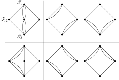
Figure 22. The additional (other than the single diamond) possible $N({\mathcal{T}}_{1},{\mathcal{T}}_{2})$ in type $C_{n}$, when ${\mathcal{G}}_{1},{\mathcal{G}}_{2}$ are adjacent. From left to right: Split, double and heavy diamonds. In each cell, the leftmost vertices are ${\mathcal{T}}_{1}$, ${\mathcal{T}}_{12}$ and ${\mathcal{T}}_{2}$, as in the first cell.

Note that, in this case, exactly one of ${\mathcal{G}}_{1},{\mathcal{G}}_{2}$ is a neutral clover and the other is an adjacent neutral triangle. Suppose that the loop game $\ell$ in ${\mathcal{D}}$ is played by vertex $x$ and that the other two vertices in ${\mathcal{D}}$ are $y,z$. Note that any way of reversing ${\mathcal{D}}$ in two steps will involve reversing $\ell$ exactly once, and so each path of length two from ${\mathcal{T}}_{1}$ to ${\mathcal{T}}_{2}$ will contain exactly one double edge.

The four cases in the second and third columns in Figure 22 can be seen by considering the other games played between $x,y$ and $x,z$ that are not in ${\mathcal{D}}$. Depending on their outcomes, each such game either creates a clover with loop $\ell$ at $x$ or else forms a neutral triangle together with the two “opposite” games in ${\mathcal{D}}$. After this clover/triangle is reversed, the triangle/clover, which was not initially, becomes present. See Figure 23.

Figure 23. Reversing when $\pi({\mathcal{D}})$ is a hanger in type $C_{n}$. Each row corresponds to a possible configuration for ${\mathcal{D}}$.

The proof is complete. ∎

5.2. Extended networks

Lemmas 14 and 16 above classify the types of interchange networks $N({\mathcal{T}}_{1},{\mathcal{T}}_{2})$. Recall that such a network contains all paths of length two between ${\mathcal{T}}_{1},{\mathcal{T}}_{2}$.

Definition 17.

We define the extended interchange network $\hat{N}({\mathcal{T}}_{1},{\mathcal{T}}_{2})$ to be the union of $N({\mathcal{T}}_{1}^{\prime},{\mathcal{T}}_{2}^{\prime})$ over all “antipodal” pairs ${\mathcal{T}}_{1}^{\prime},{\mathcal{T}}_{2}^{\prime}$ in $N({\mathcal{T}}_{1},{\mathcal{T}}_{2})$ at distance two.

Single, double and quadruple diamonds are “stable,” in the sense that $\hat{N}=N$. In contrast, split and heavy diamond networks extend to a type of structure, which we call a crystal. See Figure 24.

Figure 24. The crystal extended interchange network.

Remark.

All of the interchange networks that we have described, except the single diamond, can be found in Figure 3 above. This demonstrates how interchange networks can overlap and mesh together to form the interchange graph of a given score sequence.

Lemma 18.

Suppose that ${\mathcal{T}}_{1},{\mathcal{T}}_{2}$ are at distance two in ${\rm IntGr}(\Phi,{\bf s})$. Let $N=N({\mathcal{T}}_{1},{\mathcal{T}}_{2})$ and $\hat{N}=\hat{N}({\mathcal{T}}_{1},{\mathcal{T}}_{2})$.

1. If $N$ is a single, double or quadruple diamond, then the extended interchange network $\hat{N}=N$.

2. Otherwise, if $N$ is a split or heavy diamond, then the extended interchange network $\hat{N}$ is a crystal.

Proof.

Statement (1) is clear, and can be seen by inspection. On the other hand, statement (2) follows by repeated application of Lemma 16, considering the various antipodal pairs in $N$.

Case 1. If $N$ is a split diamond, as in the first column of Figure 22, then consider ${\mathcal{T}}_{1}^{\prime},{\mathcal{T}}_{2}^{\prime}$ in $N$ that are incident to only single edges in $N$. By Lemma 16, it follows that $N({\mathcal{T}}_{1}^{\prime},{\mathcal{T}}_{2}^{\prime})$ is a split diamond, and therefore $\hat{N}$ is a crystal.

Case 2. If $N$ is a heavy diamond, as in the third column of Figure 22, then consider ${\mathcal{T}}_{1}^{\prime},{\mathcal{T}}_{2}^{\prime}$ in $N$, each of which incident to exactly one single edge and one double edge in $N$. By Lemma 16, it follows that $N({\mathcal{T}}_{1}^{\prime},{\mathcal{T}}_{2}^{\prime})$ is a split diamond, and therefore there is a path of length two between them consisting of two single edges in $\hat{N}$. Then, applying Lemma 16, once again, but this time to the midpoint ${\mathcal{T}}_{12}^{\prime}$ along this path and ${\mathcal{T}}_{3}$ in $N$ that is incident to two single edges in $N$, we find that $\hat{N}$ is a crystal, as claimed. ∎

Recall that two generators are either disjoint or have exactly one game in common. A similar property holds for extended networks.

Lemma 19.

Any two distinct extended networks $\hat{N}\neq\hat{N}^{\prime}$ are either edge-disjoint or have exactly one single or double edge in common.

Proof.

By Lemma 18 there are only four types of extended networks. By an elementary case analysis, it can be seen that any two antipodal (distance two) vertices ${\mathcal{T}}_{1},{\mathcal{T}}_{2}$ in an extended network $\hat{N}$ give rise to the same extended network $\hat{N}$. That is, $\hat{N}=\hat{N}({\mathcal{T}}_{1},{\mathcal{T}}_{2})$, for any such ${\mathcal{T}}_{1},{\mathcal{T}}_{2}$. From this observation the result follows, since if two extended networks $\hat{N},\hat{N}^{\prime}$ share at least three vertices, then they necessarily have at least one antipodal pair of vertices in common. ∎

5.3. Properties of crystals

In this section, we obtain two key properties of crystals, which will play a crucial role in the type $C_{n}$ couplings discussed in Section 6.2 below.

First, we note that crystals cannot share a single edge. We will use this, together with Lemma 19, to extend certain local couplings to a consistent, global coupling.

Lemma 20.

Suppose that $\hat{N}\neq\hat{N}^{\prime}$ are distinct crystals in an interchange network ${\rm IntGr}(C_{n},{\bf s})$. Then $\hat{N}$, $\hat{N}^{\prime}$ are either edge-disjoint or share a double edge. That is, no such $\hat{N}\neq\hat{N}^{\prime}$ share a single edge.

Proof.

By the proof of Lemmas 16 and 18, it can be seen that each crystal is associated with three players. Each double edge in the crystal corresponds to reversing a neutral clover involving two of them, and each single edge corresponds to reversing a neutral triangle involving all three.

By Lemma 19, it suffices to show that two crystals $\hat{N}\neq\hat{N}^{\prime}$ cannot share a single edge. To see this, simply note that otherwise both tournaments joined by this single edge would contain a tournament on three players with three neutral triangles, which is impossible. See Figure 25. ∎

Figure 25. It is impossible for two (distinct) crystals to share a single edge, as depicted above, since there are at most two neutral triangles on any given three players in a tournament. However, each of the two “middle” vertices in this figure are incident to three single edges.

The previous result shows that single edges can be in at most one crystal. Double edges, on the other hand, can be in more than one. The following result gives an upper bound on this number, which is related to the re-weighting $w$ of the graph metric, discussed in Section 6.2, under which our coupling will be contractive.

Recall that $d=d(C_{n},{\bf s})$ is the degree of ${\rm IntGr}(C_{n},{\bf s})$.

Lemma 21.

Any given double edge in an interchange network ${\rm IntGr}(C_{n},{\bf s})$ is contained in at most $\min\{d,2n\}$ crystals.

Proof.

Consider a double edge between some ${\mathcal{T}}_{1},{\mathcal{T}}_{2}$. By Lemma 19, each crystal containing it corresponds to an additional double edge or two single edges incident to ${\mathcal{T}}_{1}$. It follows that there are at most $(d-2)/2$ such crystals.

The second bound is somewhat more complicated. Recall, as noted in the proof of Lemma 20, that each crystal is associated with three players. Suppose that a double edge between some ${\mathcal{T}}_{1},{\mathcal{T}}_{2}$ is associated with a neutral clover involving players $i,j$. We claim that, for any other player $k$, there are at most two crystals associated with $i,j,k$. To see this, observe that, if there were three, then one of ${\mathcal{T}}_{1},{\mathcal{T}}_{2}$ would be incident to four single edges in these crystals. However, this would imply that in one of ${\mathcal{T}}_{1},{\mathcal{T}}_{2}$ there are four neutral triangles on $i,j,k$, which is impossible. Indeed, as noted in the proof of Lemma 20, there can be at most two. Therefore, there are at most $2(n-2)$ crystals containing any given double edge. (In fact, the upper bound $n-2$ can be proved, but involves a more careful analysis.) ∎

6. Rapid mixing

Using the results of the previous section, we show that simple random walk on any given ${\rm IntGr}(\Phi,{\bf s})$ is rapidly mixing. The idea is to first define local couplings on extended networks $\hat{N}$. We then argue that these local couplings are compatible, and extend to a global coupling.

In types $B_{n}$ and $D_{n}$, rapid mixing then follows by Theorem 2, using the standard weighting $w=\delta$ given by the graph distance $\delta$ in ${\rm IntGr}(\Phi,{\bf s})$. In type $C_{n}$, we will need to select a special re-weighting $w\neq\delta$, accounting for the presence of crystals in the interchange graphs of this type.

For a tournament ${\mathcal{T}}\in{\rm Tour}(\Phi,{\bf s})$, we let ${\mathcal{E}}({\mathcal{T}})$ denote the set of edges in ${\rm IntGr}(\Phi,{\bf s})$ incident to $v({\mathcal{T}})$.

6.1. Coupling in $B_{n}$ and $D_{n}$

We begin with the simplest cases of types $B_{n}$ and $D_{n}$. These types are the most straightforward, since then all networks $N({\mathcal{T}}_{1},{\mathcal{T}}_{2})$ are single diamonds, and no re-weighting of the graph metric is necessary.

Theorem 22.

Let $\Phi=B_{n}$ or $D_{n}$. Fix any ${\bf s}\in{\rm Score}(\Phi)$. Then lazy simple random walk $({\mathcal{T}}_{n}:n\geqslant 0)$ on the Coxeter interchange graph ${\rm IntGr}(\Phi,{\bf s})$ is rapidly mixing in time $t_{\rm mix}=O(d\log n)$.

Proof.

Let $\Phi=B_{n}$ or $D_{n}$. Consider two copies of lazy simple random walk $({\mathcal{T}}_{n}^{\prime})$ and $({\mathcal{T}}_{n}^{\prime\prime})$ on ${\rm IntGr}(\Phi,{\bf s})$, started from neighboring ${\mathcal{T}}_{0}^{\prime},{\mathcal{T}}_{0}^{\prime\prime}\in{\rm Tour}(\Phi,{\bf s})$. Then ${\mathcal{T}}_{0}^{\prime\prime}={\mathcal{T}}_{0}^{\prime}*{\mathcal{G}}$ for some type $\Phi$ generator ${\mathcal{G}}\subset{\mathcal{T}}_{0}^{\prime}$. In this sense, the random walks start at distance 1.

We will construct a contractive coupling of ${\mathcal{T}}_{1}^{\prime},{\mathcal{T}}_{1}^{\prime\prime}$, such that the expected distance between ${\mathcal{T}}_{1}^{\prime},{\mathcal{T}}_{1}^{\prime\prime}$ is strictly less than $1$, uniformly in the choice of ${\mathcal{T}}_{0}^{\prime},{\mathcal{T}}_{0}^{\prime\prime}$. In fact, in this coupling, the ${\mathcal{T}}_{1}^{\prime},{\mathcal{T}}_{1}^{\prime\prime}$ will coincide with probability $1/d$, and otherwise remain at distance $1$.

More specifically, we couple ${\mathcal{T}}_{1}^{\prime},{\mathcal{T}}_{1}^{\prime\prime}$ using the natural bijection $\psi$ from ${\mathcal{E}}({\mathcal{T}}_{0}^{\prime})$ to ${\mathcal{E}}({\mathcal{T}}_{0}^{\prime\prime})$, which fixes the edge $\{{\mathcal{T}}_{0}^{\prime},{\mathcal{T}}_{0}^{\prime\prime}\}$ and pairs “opposite” edges in each single diamond containing $\{{\mathcal{T}}_{0}^{\prime},{\mathcal{T}}_{0}^{\prime\prime}\}$. By Lemmas 14 and 16, for each type $\Phi$ generator ${\mathcal{G}}^{\prime}\neq{\mathcal{G}}\subset{\mathcal{T}}_{0}^{\prime}$, the network $N({\mathcal{T}}_{0}^{\prime\prime},{\mathcal{T}}_{0}^{\prime}*{\mathcal{G}}^{\prime})$ is a single diamond. As such, there are exactly two paths of length two from ${\mathcal{T}}_{0}^{\prime\prime}$ to ${\mathcal{T}}_{0}^{\prime}*{\mathcal{G}}^{\prime}$. One such path passes through ${\mathcal{T}}_{0}^{\prime}$. We let

$$\psi(\{{\mathcal{T}}_{0}^{\prime},{\mathcal{T}}_{0}^{\prime}*{\mathcal{G}}^{\prime}\})=\{{\mathcal{T}}_{0}^{\prime\prime},{\mathcal{T}}_{0}^{\prime\prime}*{\mathcal{G}}^{\prime\prime}\}$$ (3)

be the first edge along the other such path. By Theorems 1, 18 and 19, $\psi$ is a bijection from ${\mathcal{E}}({\mathcal{T}}_{0}^{\prime})$ to ${\mathcal{E}}({\mathcal{T}}_{0}^{\prime\prime})$.

Finally, we define the coupling of ${\mathcal{T}}_{1}^{\prime},{\mathcal{T}}_{1}^{\prime\prime}$ as follows. Let $\{{\mathcal{T}}_{0}^{\prime},{\mathcal{T}}_{0}^{\prime}*{\mathcal{G}}^{\prime}\}$ be a uniformly random edge in ${\mathcal{E}}({\mathcal{T}}_{0}^{\prime})$ and $r_{0}$ a Bernoulli$(1/2)$ random variable (i.e., a fair “coin flip”). If ${\mathcal{G}}^{\prime}={\mathcal{G}}$, we put ${\mathcal{T}}_{1}^{\prime}={\mathcal{T}}_{1}^{\prime\prime}={\mathcal{T}}_{0}^{\prime}$ if $r_{0}=0$ and ${\mathcal{T}}_{1}^{\prime}={\mathcal{T}}_{1}^{\prime\prime}={\mathcal{T}}_{0}^{\prime\prime}$ if $r_{0}=1$. In this case, the coupling contracts. On the other hand, if ${\mathcal{G}}^{\prime}\neq{\mathcal{G}}$ we put ${\mathcal{T}}_{1}^{\prime}={\mathcal{T}}_{0}^{\prime}$ and ${\mathcal{T}}_{1}^{\prime\prime}={\mathcal{T}}_{0}^{\prime\prime}$ if $r_{0}=0$, and ${\mathcal{T}}_{1}^{\prime}={\mathcal{T}}_{0}^{\prime}*{\mathcal{G}}^{\prime}$ and ${\mathcal{T}}_{1}^{\prime\prime}={\mathcal{T}}_{0}^{\prime\prime}*{\mathcal{G}}^{\prime\prime}$ if $r_{0}=1$, where ${\mathcal{G}}^{\prime\prime}$ is given by the bijection $\psi$ in (3). See Figure 26.

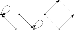
Figure 26. A contractive coupling in $B_{n}$ and $D_{n}$. The black and white vertices represent the starting positions ${\mathcal{T}}_{0}^{\prime},{\mathcal{T}}_{0}^{\prime\prime}$. In the configuration at right, corresponding to ${\mathcal{G}}^{\prime}\neq{\mathcal{G}}$, the loops have been omitted, since in this case the walks are either both lazy or not.

In this coupling, ${\mathcal{T}}_{1}^{\prime}={\mathcal{T}}_{1}^{\prime\prime}$ with probability $1/d$. Otherwise, they remain at distance $1$. By Theorem 4, the diameter of ${\rm IntGr}(\Phi,{\bf s})$ is $D=O(n^{2})$. Therefore, by Theorem 2, the mixing time is bounded by $O(d\log n)$. ∎

Remark.

Rapid mixing for classical (type $A_{n-1}$) tournaments follows as a special case of the argument above.

6.2. Coupling in $C_{n}$

Finally, we investigate mixing in type $C_{n}$.

Recall that, in types $B_{n}$ and $D_{n}$, the coupling was determined by an edge pairing, given by a bijection $\psi$ from ${\mathcal{E}}({\mathcal{T}}_{0}^{\prime})$ to ${\mathcal{E}}({\mathcal{T}}_{0}^{\prime\prime})$, where ${\mathcal{T}}_{0}^{\prime},{\mathcal{T}}_{0}^{\prime\prime}$ are neighboring tournaments in ${\rm IntGr}(\Phi,{\bf s})$. The coupling in type $C_{n}$ is also determined by such a $\psi$, however, since there are a number of different networks in type $C_{n}$, the pairing is more involved.

The fact (see Lemma 20) that distinct crystals cannot share a single edge is crucial. Otherwise it would not be possible to extend natural local couplings on extended networks to a global coupling. Roughly speaking, this is because (see Case 1b in the proof of Theorem 23 below) single edges $\{{\mathcal{T}}_{0}^{\prime},{\mathcal{T}}_{0}^{\prime\prime}\}$ in a crystal will need to be paired with one of the edges in a double edge of the same crystal. As such, if there were two crystals with the same single edge, a bijective pairing would not be possible.

Furthermore, there is an additional complication in type $C_{n}$. As it turns out, the pairing $\psi$ does not lead to a contractive coupling, with respect to the graph distance in ${\rm IntGr}(C_{n},{\bf s})$. The problem concerns the case that the initial starting positions ${\mathcal{T}}_{0}^{\prime},{\mathcal{T}}_{0}^{\prime\prime}$ are joined by a single edge in a crystal. In this case, the natural coupling is only “neutral” (i.e., with $\alpha=0$ in Theorem 2), rather than contractive.

There are (at least) three ways to overcome this difficulty, leading to increasingly better bounds on the mixing time. The first way is to apply is to apply Bordewich and Dyer’s [3] path coupling without contraction, leading to an upper bound $O(dn^{4})=O(n^{7})$. It is also possible to apply path coupling at time $t=2$, since at this point the coupling (with respect to the usual graph metric) becomes contractive. In doing so, the key is to observe that, in the problematic case that ${\mathcal{T}}_{0}^{\prime},{\mathcal{T}}_{0}^{\prime\prime}$ are joined by a single edge in a crystal, if ${\mathcal{T}}_{1}^{\prime}$ stays within the crystal then the pairing $\psi$ (described below) selects a ${\mathcal{T}}_{1}^{\prime\prime}$ in the crystal such that ${\mathcal{T}}_{1}^{\prime},{\mathcal{T}}_{1}^{\prime\prime}$ are now joined by a double edge. This argument leads to an upper bound of $O(d^{2}\log n)=O(n^{6}\log n)$.

We will present a third strategy, by re-weighting the metric, which yields to a better bound.

Recall (see Lemma 20) that single edges in ${\rm IntGr}(C_{n},{\bf s})$ are contained in at most one crystal. Double edges, on the other hand, can be contained in more than one. We define the crystal degree of a double edge to be the number of crystals containing it. We let $\gamma=\gamma(C_{n},{\bf s})$ denote the maximal crystal degree, over all double edges. By Lemma 21, we have that $\gamma\leqslant\min\{d,2n\}$, where $d=d(C_{n},{\bf s})$ is the degree of ${\rm IntGr}(C_{n},{\bf s})$.

We will assume throughout that $\gamma>0$. Indeed, if $\gamma=0$, then there are no crystals in the interchange graph. In this case, a straightforward modification of the proof of Theorem 22 (using the standard graph metric) shows that $t_{\rm mix}=O(d\log n)$.

Using the re-weighting $w$ that puts $w=1$ on (each edge in) double edges and $1+1/\gamma$ on single edges, we will prove the following result.

Theorem 23.

Let $\Phi=C_{n}$. Fix any ${\bf s}\in{\rm Score}(\Phi)$. Then lazy simple random walk $({\mathcal{T}}_{n}:n\geqslant 0)$ on the Coxeter interchange graph ${\rm IntGr}(C_{n},{\bf s})$ is rapidly mixing. If there are no crystals in ${\rm IntGr}(C_{n},{\bf s})$ (when $\gamma=0$) then $t_{\rm mix}=O(d\log n)$. Otherwise, we have $t_{\rm mix}=O(\gamma d\log n)$.

In particular, this result implies that $t_{\rm mix}=O(n^{4}\log n)$.

Proof.

As discussed, let us assume that $\gamma>0$, as otherwise a simple adaptation of the general reasoning in types $B_{n}$ and $D_{n}$ (the proof of Theorem 22) shows that $t_{\rm mix}=O(d\log n)$.

Consider two copies of lazy simple random walk $({\mathcal{T}}_{n}^{\prime})$ and $({\mathcal{T}}_{n}^{\prime\prime})$ on ${\rm IntGr}(C_{n},{\bf s})$, started from neighbors ${\mathcal{T}}_{0}^{\prime},{\mathcal{T}}_{0}^{\prime\prime}\in{\rm Tour}(C_{n},{\bf s})$. Let ${\mathcal{G}}$ be such that ${\mathcal{T}}_{0}^{\prime\prime}={\mathcal{T}}_{0}^{\prime}*{\mathcal{G}}$.

The first step is to obtain an edge pairing $\psi$, which will associate a ${\mathcal{T}}_{1}^{\prime\prime}$ to each possible ${\mathcal{T}}_{1}^{\prime}$. Then we will show that this coupling is contractive, with respect to the re-weighting $w=1+1/\gamma$ on single edges and $w=1$ on each edge in double edges. The key in this regard will be the classification of extended networks, established in Section 5.

By Lemma 20, there are three cases to consider:

1. ${\mathcal{G}}=\Delta$ is a neutral triangle, and the edge $\{{\mathcal{T}}_{0}^{\prime},{\mathcal{T}}_{0}^{\prime\prime}\}$ is in

   1. no crystal,

   2. exactly one crystal.

2. ${\mathcal{G}}=\Theta$ is a neutral clover, and the double edge between ${\mathcal{T}}_{0}^{\prime},{\mathcal{T}}_{0}^{\prime\prime}$ is in $\gamma^{\prime}\leqslant\gamma$ crystals.

In these cases, we will construct couplings with the following properties:

• In Case 1a, either ${\mathcal{T}}_{1}^{\prime}={\mathcal{T}}_{1}^{\prime\prime}$, or else ${\mathcal{T}}_{1}^{\prime},{\mathcal{T}}_{1}^{\prime\prime}$ are again joined by a single edge.

• In Case 1b, either ${\mathcal{T}}_{1}^{\prime},{\mathcal{T}}_{1}^{\prime\prime}$ are joined by a double edge in the crystal, or else ${\mathcal{T}}_{1}^{\prime},{\mathcal{T}}_{1}^{\prime\prime}$ are joined by a single edge.

• In Case 2, either ${\mathcal{T}}_{1}^{\prime},{\mathcal{T}}_{1}^{\prime\prime}$ are joined by a single edge in some crystal containing the double edge between ${\mathcal{T}}_{0}^{\prime},{\mathcal{T}}_{0}^{\prime\prime}$, or else ${\mathcal{T}}_{1}^{\prime},{\mathcal{T}}_{1}^{\prime\prime}$ are joined by a double edge.

Note that, under these couplings, crystal networks work like “switches,” in that they move single edges to double edges, and vice versa. Also note that, it is Cases 1b and 2 in which the choice of $w$ is crucial. We put weight $w=1+1/\gamma$ on single edges so that, as we will see, the couplings in these cases are contractive.

Case 1a. Suppose that ${\mathcal{G}}=\Delta$ is a neutral triangle, and that the single edge $\{{\mathcal{T}}_{0}^{\prime},{\mathcal{T}}_{0}^{\prime\prime}\}$ is not contained in a crystal. Then, by Lemmas 14 and 16, all extended networks $\hat{N}$ containing $\{{\mathcal{T}}_{0}^{\prime},{\mathcal{T}}_{0}^{\prime\prime}\}$ are single and double diamonds. As such, it is only slightly more complicated to construct a contractive coupling in this case, than it was in types $B_{n}$ and $D_{n}$ above. We proceed as depicted in Figure 27 (cf. Figure 26).

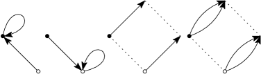
Figure 27. Case 1a: A contractive coupling, when the starting positions (black and white vertices) are joined by a single edge, which is not in a crystal.

Once again (as in the proof of Theorem 22), using Theorems 1, 18 and 19, we find a bijection $\psi$ from from ${\mathcal{E}}({\mathcal{T}}_{0}^{\prime})$ to ${\mathcal{E}}({\mathcal{T}}_{0}^{\prime\prime})$ that fixes the edge $\{{\mathcal{T}}_{0}^{\prime},{\mathcal{T}}_{0}^{\prime\prime}\}$ and pairs “opposite” edges in single and double diamonds containing $\{{\mathcal{T}}_{0}^{\prime},{\mathcal{T}}_{0}^{\prime\prime}\}$. and so correspond to the same generator.

For each edge $\{{\mathcal{T}}_{0}^{\prime},{\mathcal{T}}_{0}^{\prime}*{\mathcal{G}}^{\prime}\}$ in a single diamond $\hat{N}$ containing $\{{\mathcal{T}}_{0}^{\prime},{\mathcal{T}}_{0}^{\prime\prime}\}$, we let

$$\psi(\{{\mathcal{T}}_{0}^{\prime},{\mathcal{T}}_{0}^{\prime}*{\mathcal{G}}^{\prime}\})=\{{\mathcal{T}}_{0}^{\prime\prime},{\mathcal{T}}_{0}^{\prime\prime}*{\mathcal{G}}^{\prime\prime}\}$$ (4)

be the “opposite” edge in $\hat{N}$.

Likewise, for each double edge, consisting of two copies $\{{\mathcal{T}}_{0}^{\prime},{\mathcal{T}}_{0}^{\prime}*{\mathcal{G}}^{\prime}\}^{(i)}$, with $i\in\{1,2\}$, of the same edge in a double diamond network $\hat{N}$ containing $\{{\mathcal{T}}_{0}^{\prime},{\mathcal{T}}_{0}^{\prime\prime}\}$, we let

$$\psi(\{{\mathcal{T}}_{0}^{\prime},{\mathcal{T}}_{0}^{\prime}*{\mathcal{G}}^{\prime}\}^{(i)})=\{{\mathcal{T}}_{0}^{\prime\prime},{\mathcal{T}}_{0}^{\prime\prime}*{\mathcal{G}}^{\prime\prime}\}^{(i)},$$ (5)

with $i\in\{1,2\}$, be the “opposite” edges in $\hat{N}$.

We couple ${\mathcal{T}}_{1}^{\prime},{\mathcal{T}}_{1}^{\prime\prime}$ as follows. Let $\{{\mathcal{T}}_{0}^{\prime},{\mathcal{T}}_{0}^{\prime}*{\mathcal{G}}^{\prime}\}$ be a uniformly random edge in ${\mathcal{E}}({\mathcal{T}}_{0}^{\prime})$ and $r_{0}$ a Bernoulli$(1/2)$. (Note that, this is a uniformly random edge, not generator. Indeed, neutral clovers ${\mathcal{G}}^{\prime}=\Theta$ corresponding to double edges are twice as likely to be selected as neutral triangles ${\mathcal{G}}^{\prime}=\Delta$.) If ${\mathcal{G}}^{\prime}={\mathcal{G}}$, we put ${\mathcal{T}}_{1}^{\prime}={\mathcal{T}}_{1}^{\prime\prime}={\mathcal{T}}_{0}^{\prime}$ if $r_{0}=0$ and ${\mathcal{T}}_{1}^{\prime}={\mathcal{T}}_{1}^{\prime\prime}={\mathcal{T}}_{0}^{\prime\prime}$ if $r_{0}=1$. On the other hand, if ${\mathcal{G}}^{\prime}\neq{\mathcal{G}}$, we put ${\mathcal{T}}_{1}^{\prime}={\mathcal{T}}_{0}^{\prime}$ and ${\mathcal{T}}_{1}^{\prime\prime}={\mathcal{T}}_{0}^{\prime\prime}$ if $r_{0}=0$ and ${\mathcal{T}}_{1}^{\prime}={\mathcal{T}}_{0}^{\prime}*{\mathcal{G}}^{\prime}$ and ${\mathcal{T}}_{1}^{\prime\prime}={\mathcal{T}}_{0}^{\prime\prime}*{\mathcal{G}}^{\prime\prime}$ if $r_{0}=1$, where ${\mathcal{G}}^{\prime\prime}$ is given by the bijection $\psi$, defined in (4) or (5) above.

Note that ${\mathcal{T}}_{1}^{\prime}={\mathcal{T}}_{1}^{\prime\prime}$ with probability $1/d$. Otherwise, ${\mathcal{T}}_{1}^{\prime},{\mathcal{T}}_{1}^{\prime\prime}$ are again joined by a single edge. As such

$${\mathbb{E}}[w({\mathcal{T}}_{1}^{\prime},{\mathcal{T}}_{1}^{\prime\prime})]=(1-1/d)w({\mathcal{T}}_{0}^{\prime},{\mathcal{T}}_{0}^{\prime\prime}).$$ (6)

Case 1b. Suppose that ${\mathcal{G}}=\Delta$ is a neutral triangle, and that the single edge $\{{\mathcal{T}}_{0}^{\prime},{\mathcal{T}}_{0}^{\prime\prime}\}$ is contained in exactly one crystal. Once again, by Lemma 19, all single and double diamonds and the one crystal containing $\{{\mathcal{T}}_{0}^{\prime},{\mathcal{T}}_{0}^{\prime\prime}\}$ are otherwise edge-disjoint. In this case, the bijection can no longer fix $\{{\mathcal{T}}_{0}^{\prime},{\mathcal{T}}_{0}^{\prime\prime}\}$, as in Case 1a. Rather, we will need to use this edge in a non-trivial way in order to define the edge pairing within the crystal.

The bijection $\psi$, in this case, is defined in the same way as in Case 1a for the edges in each single and double diamond. On the other hand, for the edges in the crystal, we define $\psi$ as indicated in Figure 28. That is, the two single edges in the crystal incident to ${\mathcal{T}}_{0}^{\prime}$ (one of which is $\{{\mathcal{T}}_{0}^{\prime},{\mathcal{T}}_{0}^{\prime\prime}\}$) are paired with the double edges in the crystal incident to ${\mathcal{T}}_{0}^{\prime\prime}$, and vice versa. By Theorem 1, $\psi$ is a bijection from ${\mathcal{E}}({\mathcal{T}}_{0}^{\prime})$ to ${\mathcal{E}}({\mathcal{T}}_{0}^{\prime\prime})$. We stress here that $\psi$ pairs edges, not generators, and it is critical, in this case, that there is only one crystal containing $\{{\mathcal{T}}_{0}^{\prime},{\mathcal{T}}_{0}^{\prime\prime}\}$ (since it can only be paired once).

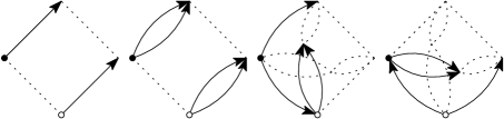
Figure 28. Case 1b: A neutral coupling, when the starting positions (black and white vertices) are joined by a single edge, which is in exactly one crystal. Note that, if the walks stay in the crystal, they move to a pair joined by a double edge.

To couple ${\mathcal{T}}_{1}^{\prime},{\mathcal{T}}_{1}^{\prime\prime}$, we let $\{{\mathcal{T}}_{0}^{\prime},{\mathcal{T}}_{0}^{\prime}*{\mathcal{G}}^{\prime}\}$ be a uniformly random edge in ${\mathcal{E}}({\mathcal{T}}_{0}^{\prime})$ and $r_{0}$ a Bernoulli$(1/2)$. If $r_{0}=0$, we put ${\mathcal{T}}_{1}^{\prime}={\mathcal{T}}_{0}^{\prime}$ and ${\mathcal{T}}_{1}^{\prime\prime}={\mathcal{T}}_{0}^{\prime\prime}$. If $r_{0}=1$, we put ${\mathcal{T}}_{1}^{\prime}={\mathcal{T}}_{0}^{\prime}*{\mathcal{G}}^{\prime}$ and ${\mathcal{T}}_{1}^{\prime\prime}={\mathcal{T}}_{0}^{\prime\prime}*{\mathcal{G}}^{\prime\prime}$, where ${\mathcal{G}}^{\prime\prime}$ is given by the bijection $\psi$.

In this case, with probability $2/d$ the pair ${\mathcal{T}}_{1}^{\prime},{\mathcal{T}}_{1}^{\prime\prime}$ remains in the crystal, but are now joined by a double edge. Otherwise, ${\mathcal{T}}_{1}^{\prime},{\mathcal{T}}_{1}^{\prime\prime}$ are again joined by a single edge. Therefore,

$${\mathbb{E}}[w({\mathcal{T}}_{1}^{\prime},{\mathcal{T}}_{1}^{\prime\prime})] =(1-2/d)(1+1/\gamma)+2/d$$

$$=\left[1-\frac{2}{d(1+\gamma)}\right]w({\mathcal{T}}_{0}^{\prime},{\mathcal{T}}_{0}^{\prime\prime}),$$ (7)

since $w({\mathcal{T}}_{0}^{\prime},{\mathcal{T}}_{0}^{\prime\prime})=1+1/\gamma$.

Case 2. Finally, suppose that ${\mathcal{G}}=\Theta$ is a neutral clover. Suppose that $\{{\mathcal{T}}_{0}^{\prime},{\mathcal{T}}_{0}^{\prime\prime}\}$ is contained in $\gamma^{\prime}\leqslant\gamma$ crystals.

By Lemmas 14 and 16, all extended networks $\hat{N}$ containing $\{{\mathcal{T}}_{0}^{\prime},{\mathcal{T}}_{0}^{\prime\prime}\}$ are double and quadruple diamonds and crystals. As in the previous cases, we define $\psi$ in this case by pairing “opposite” edges in the double and quadruple diamonds. In this case, $\psi$ fixes the two edges in the double edge between ${\mathcal{T}}_{0}^{\prime},{\mathcal{T}}_{0}^{\prime\prime}$. Note that if $\{{\mathcal{T}}_{0}^{\prime},{\mathcal{T}}_{0}^{\prime\prime}\}$ is in a crystal, then one of ${\mathcal{T}}_{0}^{\prime},{\mathcal{T}}_{0}^{\prime\prime}$ is incident to two single edges in the crystal and the other is incident to a double edge $\neq\{{\mathcal{T}}_{0}^{\prime},{\mathcal{T}}_{0}^{\prime\prime}\}$ in the crystal. We define $\psi$ on each such crystal by pairing these edges, as indicated in Figure 29. Once again, applying Theorem 1, we see that $\psi$ is a bijection from ${\mathcal{E}}({\mathcal{T}}_{0}^{\prime})$ to ${\mathcal{E}}({\mathcal{T}}_{0}^{\prime\prime})$.

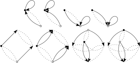
Figure 29. Case 2: A contractive coupling, when the starting positions (black and white vertices) are joined by a double edge.

To couple ${\mathcal{T}}_{1}^{\prime},{\mathcal{T}}_{1}^{\prime\prime}$, we let $\{{\mathcal{T}}_{0}^{\prime},{\mathcal{T}}_{0}^{\prime}*{\mathcal{G}}^{\prime}\}$ be a uniformly random edge in ${\mathcal{E}}({\mathcal{T}}_{0}^{\prime})$ and $r_{0}$ a Bernoulli$(1/2)$. If ${\mathcal{G}}^{\prime}={\mathcal{G}}$, we put ${\mathcal{T}}_{1}^{\prime}={\mathcal{T}}_{1}^{\prime\prime}={\mathcal{T}}_{0}^{\prime}$ if $r_{0}=0$ and ${\mathcal{T}}_{1}^{\prime}={\mathcal{T}}_{1}^{\prime\prime}={\mathcal{T}}_{0}^{\prime\prime}$ if $r_{0}=1$. Otherwise, if ${\mathcal{G}}^{\prime}\neq{\mathcal{G}}$, we put ${\mathcal{T}}_{1}^{\prime}={\mathcal{T}}_{0}^{\prime}$ and ${\mathcal{T}}_{1}^{\prime\prime}={\mathcal{T}}_{0}^{\prime\prime}$ if $r_{0}=0$ and ${\mathcal{T}}_{1}^{\prime}={\mathcal{T}}_{0}^{\prime}*{\mathcal{G}}^{\prime}$ and ${\mathcal{T}}_{1}^{\prime\prime}={\mathcal{T}}_{0}^{\prime\prime}*{\mathcal{G}}^{\prime\prime}$ if $r_{0}=1$, where ${\mathcal{G}}^{\prime\prime}$ is given by the bijection $\psi$.

In this case, ${\mathcal{T}}_{1}^{\prime}={\mathcal{T}}_{1}^{\prime\prime}$ with probability $2/d$. With probability $\gamma^{\prime}/d$, the pair ${\mathcal{T}}_{1}^{\prime},{\mathcal{T}}_{1}^{\prime\prime}$ move within one of the $\gamma^{\prime}$ crystals containing $\{{\mathcal{T}}_{0}^{\prime},{\mathcal{T}}_{0}^{\prime\prime}\}$, and are then joined by a single edge. Otherwise, with probability $1-(2+\gamma^{\prime})/d$, ${\mathcal{T}}_{1}^{\prime},{\mathcal{T}}_{1}^{\prime\prime}$ remain joined by a double edge. Therefore,

$${\mathbb{E}}[w({\mathcal{T}}_{1}^{\prime},{\mathcal{T}}_{1}^{\prime\prime})] =\frac{\gamma^{\prime}}{d}(1+1/\gamma)+1-\frac{2+\gamma^{\prime}}{d}$$

$$=1-\frac{2\gamma-\gamma^{\prime}}{d\gamma}$$

$$\leqslant(1-1/d)w({\mathcal{T}}_{0}^{\prime},{\mathcal{T}}_{0}^{\prime\prime}),$$ (8)

since $w({\mathcal{T}}_{0}^{\prime},{\mathcal{T}}_{0}^{\prime\prime})=1$.

By (6)–(8), we may apply Theorem 2 with $\alpha=O(1/\gamma d)$. Note that, by Theorem 4, it follows that $D_{w}=O((1+1/\gamma)D)=O(n^{2})$. We conclude that the mixing time is bounded by $O(\gamma d\log n)$, as claimed. ∎

References

- 1. D. Aldous and J. A. Fill, Reversible markov chains and random walks on graphs, 2002, Unfinished monograph, recompiled 2014, available at http://www.stat.berkeley.edu/~aldous/RWG/book.html.
- 2. F. Ardila, F. Castillo, C. Eur, and A. Postnikov, Coxeter submodular functions and deformations of Coxeter permutahedra, Adv. Math. 365 (2020), 107039, 36.
- 3. M. Bordewich and M. Dyer, Path coupling without contraction, J. Discrete Algorithms 5 (2007), no. 2, 280–292.
- 4. R. A. Brualdi and Q. Li, The interchange graph of tournaments with the same score vector, Progress in graph theory (Waterloo, Ont., 1982), Academic Press, Toronto, ON, 1984, pp. 129–151.
- 5. R. Bubley and M. Dyer, Path coupling: A technique for proving rapid mixing in Markov chains, Proc. 38th IEEE Symposium on Foundations of Computer Science, IEEE Computer Society Press, 1997, pp. 223–231.
- 6. E. Cartan, Sur la Reduction a sa Forme Canonique de la Structure d’un Groupe de Transformations Fini et Continu, Amer. J. Math. 18 (1896), no. 1, 1–61.
- 7. A.-H. Chen, J.-M. Chang, and Y.-L. Wang, The interchange graphs of tournaments with minimum score vectors are exactly hypercubes, Graphs Combin. 25 (2009), no. 1, 27–34.
- 8. B. Hall, Lie groups, Lie algebras, and representations, second ed., Graduate Texts in Mathematics, vol. 222, Springer, Cham, 2015, An elementary introduction.
- 9. J. E. Humphreys, Reflection groups and Coxeter groups, Cambridge Studies in Advanced Mathematics, vol. 29, Cambridge University Press, Cambridge, 1990.
- 10. M. Isaev, T. Iyer, and B. D. McKay, Asymptotic enumeration of orientations of a graph as a function of the out-degree sequence, Electron. J. Combin. 27 (2020), no. 1, Paper No. 1.26, 30.
- 11. R. Kannan, P. Tetali, and S. Vempala, Simple Markov-chain algorithms for generating bipartite graphs and tournaments, Random Structures Algorithms 14 (1999), no. 4, 293–308.
- 12. W. Killing, Die Zusammensetzung der stetigen endlichen Transformationsgruppen, Math. Ann. 36 (1890), no. 2, 161–189.
- 13. B. Kolesnik, R. Mitchell, and T. Przybyłowski, Tournaments on signed graphs, preprint available at arXiv:2312.04532.
- 14. B. Kolesnik and M. Sanchez, Coxeter tournaments, preprint available at arXiv:2302.14002.
- 15. by same author, The geometry of random tournaments, Discrete Comput. Geom., in press, available at https://doi.org/10.1007/s00454-023-00571-4.
- 16. H. G. Landau, On dominance relations and the structure of animal societies. III. The condition for a score structure, Bull. Math. Biophys. 15 (1953), 143–148.
- 17. D. A. Levin, Y. Peres, and E. L. Wilmer, Markov chains and mixing times, American Mathematical Society, Providence, RI, 2009, With a chapter by James G. Propp and David B. Wilson.
- 18. B. D. McKay, The asymptotic numbers of regular tournaments, Eulerian digraphs and Eulerian oriented graphs, Combinatorica 10 (1990), no. 4, 367–377.
- 19. B. D. McKay and X. Wang, Asymptotic enumeration of tournaments with a given score sequence, J. Combin. Theory Ser. A 73 (1996), no. 1, 77–90.
- 20. L. McShine, Random sampling of labeled tournaments, Electron. J. Combin. 7 (2000), Research Paper 8, 9.
- 21. J. W. Moon, An extension of Landau’s theorem on tournaments, Pacific J. Math. 13 (1963), 1343–1345.
- 22. by same author, Topics on tournaments, Holt, Rinehart and Winston, New York-Montreal, Que.-London, 1968.
- 23. A. Postnikov, Permutohedra, associahedra, and beyond, Int. Math. Res. Not. IMRN (2009), no. 6, 1026–1106.
- 24. R. Rado, An inequality, J. London Math. Soc. 27 (1952), 1–6.
- 25. S. Sarkar, Mixing times of tournaments, undergraduate thesis, Georgia Institute of Technology, 2020.
- 26. J. H. Spencer, Random regular tournaments, Period. Math. Hungar. 5 (1974), 105–120.
- 27. R. P. Stanley, Decompositions of rational convex polytopes, Ann. Discrete Math. 6 (1980), 333–342.
- 28. D. B. Wilson, Mixing times of Lozenge tiling and card shuffling Markov chains, Ann. Appl. Probab. 14 (2004), no. 1, 274–325.
- 29. T. Zaslavsky, The geometry of root systems and signed graphs, Amer. Math. Monthly 88 (1981), no. 2, 88–105.
- 30. by same author, Signed graphs, Discrete Appl. Math. 4 (1982), no. 1, 47–74.
- 31. by same author, Orientation of signed graphs, European J. Combin. 12 (1991), no. 4, 361–375.
- 32. G. M. Ziegler, Lectures on polytopes, Graduate Texts in Mathematics, vol. 152, Springer-Verlag, New York, 1995.