Self-Supervised Representation Learning for Nerve Fiber Distribution Patterns in 3D-PLI

Abstract

A comprehensive understanding of the organizational principles in the human brain requires, among other factors, well-quantifiable descriptors of nerve fiber architecture. Three-dimensional polarized light imaging (3D-PLI) is a microscopic imaging technique that enables insights into the fine-grained organization of myelinated nerve fibers with high resolution. Descriptors characterizing the fiber architecture observed in 3D-PLI would enable downstream analysis tasks such as multimodal correlation studies, clustering, and mapping. However, best practices for observer-independent characterization of fiber architecture in 3D-PLI are not yet available. To this end, we propose the application of a fully data-driven approach to characterize nerve fiber architecture in 3D-PLI images using self-supervised representation learning. We introduce a 3D-Context Contrastive Learning (CL-3D) objective that utilizes the spatial neighborhood of texture examples across histological brain sections of a 3D reconstructed volume to sample positive pairs for contrastive learning. We combine this sampling strategy with specifically designed image augmentations to gain robustness to typical variations in 3D-PLI parameter maps. The approach is demonstrated for the 3D reconstructed occipital lobe of a vervet monkey brain. We show that extracted features are highly sensitive to different configurations of nerve fibers, yet robust to variations between consecutive brain sections arising from histological processing. We demonstrate their practical applicability for retrieving clusters of homogeneous fiber architecture and performing data mining for interactively selected templates of specific components of fiber architecture such as U-fibers.

Keywords deep learning, contrastive learning, fiber architecture, polarized light imaging, occipital lobe, vervet monkey brain

1 Introduction

Decoding the human brain requires analyzing its structural and functional organization at different spatial scales, including cytoarchitecture and fiber architecture at microscopic resolutions [Amunts and Zilles, 2015, Axer and Amunts, 2022]. Three-dimensional polarized light imaging (3D-PLI) [Axer et al., 2011b] is an imaging technique that reveals the fine-grained configuration and 3D orientation of myelinated nerve fibers in both gray and white matter with micrometer resolution. 3D-PLI thus establishes a link between microscopic myeloarchitecture and dMRI-based structural connectivity at the macro- and mesoscopic scale [Zilles et al., 2016, Caspers and Axer, 2019]. 3D-PLI images provide detailed visual information for obtaining maps of fiber architecture at different scales. Based on 3D-PLI images, previous work demonstrated the detection of myelinated pathways and delineation of subfields in the human hippocampus [Zeineh et al., 2017] as well as the identification of fiber tracts and visual areas in the vervet monkey visual system [Takemura et al., 2020].

Polarized light imaging allows processing of whole-brain tissue sections and enables scanning of large tissue stacks [Axer et al., 2020a, Axer et al., 2020b, Howard et al., 2023]. However, interpretation and analysis of the complex information provided by 3D-PLI requires substantial expertise that cannot scale to the vastly increasing amount of data produced by recent high-throughput devices. Moreover, solutions for automated large-scale analysis of fiber architecture at the resolution provided by 3D-PLI have not been established so far, as it is difficult to derive reliable descriptors for characteristic fiber configurations from the data. A promising direction towards automated analysis of 3D-PLI is to reduce the complexity of the image data by finding a suitable embedding space of 3D-PLI textures. Ideally, the features in this embedding remain highly expressive regarding different fiber configurations while being robust against other sources of variation, such as histological processing effects and the relative 3D orientation of image patches.

Recent advances in self-supervised representation learning suggest using contrastive learning [Hadsell et al., 2006, van den Oord et al., 2018] to extract distinctive features from large amounts of data. The training objective here is to represent similar instances (positive pairs) as close points in the embedding space while pushing dissimilar instances (negative pairs) apart to prevent representational collapse. While other methods to prevent representational collapse have been proposed as well, such as clustering [Caron et al., 2020], distillation [Grill et al., 2020, Chen and He, 2021], information maximization [Zbontar et al., 2021] or variance preservation [Bardes et al., 2022], contrastive learning of visual representations by application or adaptation of SimCLR [Chen et al., 2020] and MoCo [He et al., 2020] is still popular in medical image analysis [Chen et al., 2022, Krishnan et al., 2022]. Due to its simplicity, we build on the SimCLR framework [Chen et al., 2020]. An application of SimCLR in cytoarchitectonic brain mapping was recently performed for histological images [Schiffer et al., 2021]. A main challenge they discovered was the tendency of models to focus more on anatomical landmarks than on features descriptive of cytoarchitecture when creating positive pairs based on data augmentations of the same image. To overcome this effect, they employ a supervised contrastive loss [Khosla et al., 2020] by defining positive pairs based on same labels and sample pairs within each brain area. Since class labels for fiber architecture in 3D-PLI are not yet available at the scale required for deep learning, an alternative strategy for generating positive pairs is required.

To overcome the need for class labels, several self-supervised learning methods were proposed to learn image feature descriptions based on spatial context, which can be used to create correlated views for contrastive learning [van den Oord et al., 2018, Chen et al., 2020, Van Gansbeke et al., 2021] or to define pre-text tasks [Doersch et al., 2015, Noroozi and Favaro, 2016, Pathak et al., 2016]. For microscopic imaging, predicting the geodesic distance between image patches along the brain surface [Spitzer et al., 2018] or the sequence of multi-resolution histopathology images [Srinidhi et al., 2022] have been proposed as pre-text tasks. Other approaches leverage the spatial continuity of images by maximizing mutual information between neighboring patches in histological images [Gildenblat and Klaiman, 2019] or satellite images [Ji et al., 2019]. They assume textures in spatial proximity to be similar and therefore aim to contrast them from texture in rather distant image parts.

In the present study, we explore self-supervised contrastive learning for inferring descriptive features of local nerve fiber distribution patterns from raw 3D-PLI measurements. To generate positive pairs of 3D-PLI texture examples, we assume that fundamental properties of local fiber architecture are typically consistent between closeby image patches. While this assumption is likely violated at boundaries between distinct structural brain areas, we assume that it holds for the largest share of closeby image patches. In contrast to previous work [Gildenblat and Klaiman, 2019, Ji et al., 2019], instead of utilizing in-plane similarity of images, we use a 3D reconstructed histological volume to access the spatial coordinates of image patches in 3D. More precisely, we extract positive pairs of image patches at closeby coordinates across tissue sections. This sampling strategy is motivated by the idea that positive pairs from different tissue sections show independently measured tissue and thus encourage the learning of features that are robust to random variations in the measurement process not descriptive of fiber architecture. We denote this 3D-informed self-supervised learning strategy as 3D-Context Contrastive Learning (CL-3D).

To verify the validity of the proposed approach, we compare in-plane (CL-2D) with cross-section (CL-3D) sampling strategies for positive pairs and show that the latter aids in learning more robust features with respect to variations between brain sections. We investigate the main factors of variations in the CL-3D features by examining their principal components. Furthermore, we study the relationship between 3D-PLI texture features and morphological measures at the macroscopic scale, using a precise automatic cortex segmentation which we developed specifically for 3D-PLI images based on a U-Net model [Ronneberger et al., 2015]. To demonstrate the applicability of the learned CL-3D features, we apply the approach to a 3D reconstruction of the occipital lobe of a vervet monkey brain. We show that the features form clusters that reflect different types of fiber architecture and are suitable for interactive instance retrieval of U-fiber structures by specifying only few example patches as a template.

The main contributions of the present study are the following:

• We propose a novel 3D-Context Contrastive Learning (CL-3D) strategy to learn a powerful feature embedding for microscopic resolution image patches from 3D-PLI.

• We present specific image augmentations for maximizing invariance of learned features with respect to typical variations in 3D-PLI images.

• We show a high sensitivity of the resulting 3D-PLI feature embeddings to fundamental configurations of nerve fibers, such as myelinated radial and tangential fibers within the cortex, fiber bundles, crossings, and fannings, as well as cortical morphology.

• Using a dataset from a vervet monkey brain, we demonstrate that the learned features are well suited for exploratory data analysis, specifically for finding clusters of similar fiber architecture and retrieving locations with specific architectural properties based on interactively chosen examples.

2 Materials and Methods

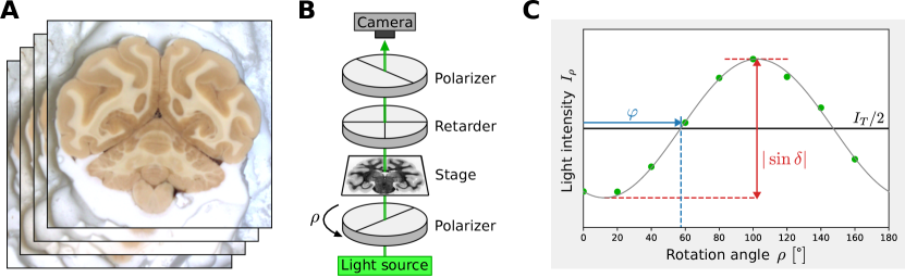
Figure 1: Overview of the 3D-PLI data acquisition. (A) Blockface images are taken for every section before slicing, providing a distortion-free reference for 3D volume reconstruction. (B) 3D-PLI measurement setup for the polarizing microscope (LMP-1) consisting of a coherent green light source, a rotating linear polarizer, a specimen stage, a stationary circular analyzer (quarter-wave retarder, linear polarizer) and a CCD camera to capture transmitted light intensities. (C) Example intensity profile recorded by a single pixel of the CCD camera at 9 polarizer rotation angles $\rho$, which can be described by three modalities: transmittance $I_{T}$, direction $\varphi$, and retardation $|\sin\delta|$.

2.1 3D-PLI measurements from the occipital lobe of a vervet monkey brain

Tissue samples.

For this study, we use a 3D reconstruction of 234 coronal sections from the right occipital lobe of a 2.4-year-old adult male vervet monkey brain (ID 1818) measured with 3D-PLI [Takemura et al., 2020]. The brain sample was obtained post-mortem after flush with phosphate-buffered saline in accordance with the Wake Forest Institutional Animal Care and Use Committee (IACUC #A11-219) and conforming the AVMA Guidelines for the Euthanasia of Animals. It was perfusion fixed with 4% paraformaldehyde, immersed in 20% glycerin for cryo-protection, and frozen at -70 C°. Sectioning of the frozen brain was performed coronally at 60 µm thickness using a large-scale cryostat microtome (Poly-cut CM 3500, Leica, Germany). Before each section was sliced, blockface images were taken as an undistorted reference for image realignment using a CCD camera (Fig. 1A).

3D-PLI acquisition.

For 3D-PLI measurement [Axer et al., 2011b, Axer et al., 2011a, Axer and Amunts, 2022], the brain sections were scanned using a polarizing microscope (LMP-1, Taorad, Germany), which provides a detailed view of the nerve fiber architecture at a resolution of 1.3 µm. In this microscope setup, sections are placed on a stage between a rotating linear polarizer and a stationary circular analyzer consisting of a quarter-wave retarder and a second linear polarizer (Fig. 1B). The setup is illuminated by an incoherent white light LED equipped with a band-pass filter of 550 $\pm$ 5 nm half-width. Variations in transmitted light intensity are captured using a CCD camera for nine equidistant rotation angles $\rho$ of the rotating linear polarizer covering 180° of rotation. The recorded light intensity variations feature sinusoidal profiles at each pixel (Fig. 1C), which are determined by the spatial orientation of myelinated nerve fibers. Using Jones calculus, a physical description for these profiles can be derived as

$$I_{\rho}=\frac{I_{T}}{2}\cdot\left(1+\sin(2\rho-2\varphi)\cdot\sin\delta\right),$$ (1)

where harmonic Fourier analysis can be applied to retrieve parameter maps of transmittance $I_{T}$, retardation $|\sin\delta|$ and direction $\varphi$ from the profiles [Axer et al., 2011a]. The phase shift $\delta$ between the ordinary and the extraordinary ray can be further decomposed as

$$\delta\approx 2\pi\frac{t\cdot\Delta n}{\lambda}\cos^{2}\alpha$$ (2)

with the cumulative thickness of birefringent tissue $t$, birefringence $\Delta n$, the wavelength of the light source $\lambda$, and nerve fiber inclination angle $\alpha$. While birefringence $\Delta n$ and wavelength $\lambda$ are kept constant for all pixels, the amount of myelinated nerve fibers, reflected by $t$, varies. To resolve Eq. 2 for inclination $\alpha$, a transmittance-weighted model [Menzel et al., 2022] can be used to estimate $t$. Fiber inclination and direction information can then be jointly visualized in fiber orientation maps in HSV color space [Axer et al., 2011b], where the hue value corresponds to in-plane fiber direction $\varphi$ while saturation and value reflect the out-of-plane fiber inclination $\alpha$ (both zero for vertical fibers at $\alpha$ = 90°).

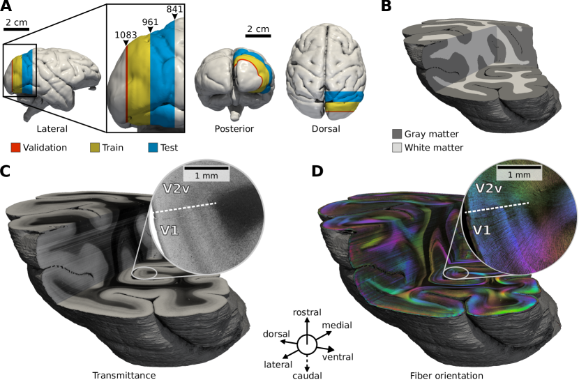
Figure 2: 3D reconstructed occipital lobe of the right hemisphere of a vervet monkey brain measured with 3D-PLI. (A) Localization of the occipital lobe on the surface of the 3D blockface reconstruction. Sections used for training (yellow), validation (red), and testing (blue) are color-coded. Numbers indicate section numbers. (B) 3D volume rendering of segmented cortical gray matter and white matter of the lobe. (C) 3D volume rendering for transmittance maps $I_{T}$ and (D) fiber orientation in HSV color space (hue: direction $\varphi$; saturation, brightness: inclination $\alpha$). Zoom-ins highlight the fiber architecture at the border between the primary visual cortex (V1) and the secondary visual cortex (V2). All volumes are masked at the pial boundary shown as a gray surface.

3D registration.

To access the three-dimensional context of images, registration of 3D-PLI parameter maps is performed on 234 sections of the right occipital lobe between from section 841 to 1083 (Fig. 2), interpolating 9 missing sections by their nearest neighbor. In order to generate an undistorted reference space, the mounted tissue block is imaged using a camera before each cutting step to obtain a full stack of blockface images for the complete specimen. A volume reconstruction is then performed from these blockface images using affine transformations (Fig. 2A), by extraction of visual markers which are positioned on the cryotome and enable precise localization of the images [Schober et al., 2015]. Subsequently, non-linear transformation fields are estimated for alignment of 3D-PLI transmittance maps using the blockface volume as reference, which yields a reconstruction of the overall anatomical shape and topology of the occipital lobe in the 3D-PLI volume space. However, blockface images do not contain sufficient structural detail for precise alignment of fine structures visible in 3D-PLI such as single fiber bundles and small blood vessels. Therefore, in a subsequent step, each 3D-PLI section (transmittance and retardation parameter maps) is iteratively mapped to its adjacent sections to reconstruct coherent 3D fiber tract transitions. All registrations are performed using the ELASTIX [Klein et al., 2010, Shamonin et al., 2014], ANTs [Avants et al., 2010, Avants et al., 2011] and ITK [McCormick et al., 2014] software packages. The computed transformation fields are used to warp all 3D-PLI parameter maps into a common volume space (Fig. 2C) with a resolution of 31077 $\times$ 28722 $\times$ 243 voxels with a voxel size of 1.3 $\times$ 1.3 $\times$ 60 µm. In-plane orientation information reflected by direction maps $\varphi$ is preserved by adjusting the 2D rotation components at each pixel estimated by the curl of the transformation field.

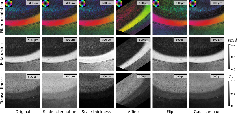
Figure 3: Illustration of implemented 3D-PLI data augmentations for an example patch from the calcarine sulcus. Images show transmittance $I_{T}$, retardation $|\sin\delta|$ and fiber orientation in HSV color space (hue: direction $\varphi$; saturation, brightness: inclination $\alpha$). The colormap for retardation is scaled with a gamma correction for visibility. Parameters for the transmittance weighted model to compute fiber orientation are kept constant for all augmentations.

2.2 Data augmentations for 3D-PLI

Data augmentations are crucial for increasing the diversity of the training data. Self-supervised contrastive learning methods in particular rely on augmentations to learn representations that are more generalizable and robust to variations in the input data [Chen et al., 2020]. It is crucial that the augmentation schemes model the expected variability adequately. In microscopy, for example, similar textures can exhibit different orientations, intensities, or sharpness in each scan. For this study, we introduce a set of augmentations specifically designed to reflect typical variations in 3D-PLI images. We derive augmentations for joint transmittance, direction, and retardation parameter maps from a physical model of 3D-PLI.

2.2.1 Modulation of signal parameters

Parameters of the tissue in the physical model of 3D-PLI might vary (e.g. transparency, thickness) depending on postmortem time, tissue processing, or storage time of the mounted sections. Here, we provide transformations that can be implemented into 3D-PLI-specific data augmentations that approximate typical variations in the parameters.

Attenuation coefficient.

The transmitted light intensity of the tissue can vary across image acquisitions due to a change in light attenuation. Assuming uniform attenuation for simplicity, the transmittance $I_{T}$ can be described by Bouguer-Lambert’s law as

$$I_{T}=I_{0}e^{-t\mu}$$ (3)

for the intensity of incident light $I_{0}$, section thickness $t$ and attenuation coefficient $\mu$. Scaling the attenuation by $\mu^{\prime}=\gamma\mu$ results in a scaled transmittance $I_{T}^{\prime}$ as follows:

$$I_{T}^{\prime}=I_{0}e^{-t\mu^{\prime}}=I_{0}(\frac{I_{T}}{I_{0}})^{\gamma}.$$ (4)

Note that this equation is only an approximation of a real change in $\mu$ due to the simplifying assumption of uniform attenuation.

Section thickness.

Although the section thickness was held constant throughout all brain sections used in this study, it might vary between data acquisitions of other samples. To reflect a relative change in thickness parameter $t$ in Eq. 2, we scale $\delta\propto t$, introducing a scaling factor $\gamma$. For retardation $r=|\sin(\delta)|$ and $\delta^{\prime}=\gamma\delta$ we obtain a scaled retardation

$$r^{\prime}=\sin(\gamma\arcsin(r)).$$ (5)

To adjust the light transmittance $I_{T}$, we compute scaled $I_{T}^{\prime}$ analog to Eq. 4 for scaled thickness $t^{\prime}=\gamma t$ as follows:

$$I_{T}^{\prime}=I_{0}e^{-t^{\prime}\mu}=I_{0}(\frac{I_{T}}{I_{0}})^{\gamma}.$$ (6)

Note that this augmentation is also only an approximation to a real change in thickness $t$, as it does not add or remove tissue components from the measurement.

2.2.2 Resampling

Many image transformations require resampling of image intensity values. For 3D-PLI, resampling of the measured intensities from Eq. 1 can be performed as

$$I^{\prime}_{\rho}=\sum_{i}w_{i}I_{\rho,i}$$ (7)

by a weighted mean of intensity values $I_{\rho,i}$ with corresponding weights $w_{i}$, where $\sum_{i}w_{i}=1$. With the 3D-PLI parameter maps, however, we work with derivations of the originally measured image intensities and cannot directly resample values for retardation $r=|\sin\delta|$ and direction values $\varphi$. By representing Eq. 7 as Fourier series and due to the linearity of the Fourier transformation, resampling of the 3D-PLI parameter maps can be performed through

$$I_{T}^{\prime} =\sum_{i}w_{i}I_{T,i}$$ (8)

$$r^{\prime}\cdot e^{\operatorname*{\mathrm{i}}2\varphi^{\prime}} =\frac{1}{I_{T}^{\prime}}\sum_{i}w_{i}r_{i}I_{T,i}\cdot e^{\operatorname*{\mathrm{i}}2\varphi_{i}},$$ (9)

by computing $I_{T}^{\prime}$ via Eq. 8 before obtaining $r^{\prime}$ and $\varphi^{\prime}$ from Eq. 9 via decomposition of the right-hand side into magnitude and phase, which correspond to $r^{\prime}$ and $2\varphi^{\prime}$, respectively. The equations are used for all geometric transformations and filters, such as affine transformations or Gaussian blur, that require resampling of 3D-PLI parameter maps.

2.2.3 Direction correction

Since 3D-PLI measures the absolute in-plane orientation of nerve fibers, any transformation that changes the geometry of image pixels requires a subsequent correction of direction values $\varphi$. For applications in diffusion MRI, Preservation of Principal Directions (PPD) [Alexander et al., 2001b, Alexander et al., 2001a] was introduced to preserve directional information undergoing non-rigid transformations. While proposed for 3D diffusion tensors, a similar correction mechanism can be introduced for 3D-PLI, where we restrict the transformations to in-plane transformations for simplicity. We convert direction angles $\varphi$ to cartesian coordinates normalized to one as

$$\vec{d}=\begin{pmatrix}\cos{\varphi}\\ \sin{\varphi}\end{pmatrix}$$ (10)

in order to generate corrected direction angles $\varphi^{\prime}$ via

$$\vec{d}^{\prime} =J_{f}\vec{d}$$ (11)

$$\varphi^{\prime} =\text{atan2}(d_{2}^{\prime},d_{1}^{\prime})$$

for non-linear image transformation function $f\colon{\mathbb{R}^{2}}\to{\mathbb{R}^{2}}$, which maps pixel coordinates in the source domain to coordinates in the target domain, and Jacobi matrix $J_{f}$ of function $f$. The correction is applied before application of function $f$ to transform the image. For specific transformations, Eq. 11 can be simplified to more convenient forms.

Rotation.

For an example of counter-clockwise rotation by arbitrary angle $\theta$, Eq. 11 can be simplified to

$$\varphi^{\prime}=\varphi+\theta.$$ (12)

Affine Transform.

For pixel coordinates $\vec{p}=[x,y]^{T}$ and an affine transformation composed of translation vector $\vec{t}$ and matrix $A$, the transformation function is given as

$$f(x,y)=A\vec{p}+\vec{t}.$$ (13)

If inserted into Eq. 11, a simplified correction mechanism for the affine transformation can be derived as

$$\vec{d}^{\prime} =A\vec{d}$$ (14)

$$\varphi^{\prime} =\text{atan2}(d_{2}^{\prime},d_{1}^{\prime}).$$

2.3 Cortex segmentation

To access brain morphology and distinguish gray and white matter locations, a U-Net model [Ronneberger et al., 2015] is trained for segmentation of pixels into background (BG), gray matter (GM), and white matter (WM) classes and applied on every 3D-PLI section. For training the model, we create a dataset representing a large variety of textures in 3D-PLI images with minimal labeling effort by employing an active learning strategy in the annotation process. Rather than annotating complete sections, we manually select 58 square regions of interest (ROIs) of size 2048 pixels (2.66 mm) from several sections, including sections outside the occipital lobe for a higher variety of examples. We train a U-Net model using these ROIs as inputs and apply the model to all available sections. We then identify the most severe misclassifications from the model outputs for selecting new ROIs. This process is repeated to obtain a growing dataset of 58, 119, 183, 301 and finally 369 ROIs of highly diverse patches capturing different textures across the entire brain.

It should be noted that large parts of the cortex can be segmented at acceptable quality using simple thresholding of transmittance and retardation values [Menzel et al., 2022]. Challenging parts, such as an oblique cut border between gray and white matter or an intersecting pial surface within narrow sulci, form only a small fraction of the data, but have a significant impact on matching inner and outer cortical boundaries. We therefore apply a multi-class implementation of focal loss [Lin et al., 2017] for the training objective to increase emphasis for the model on challenging examples. We use 3D-PLI-specific augmentations, as described in Sec. 2.2, for training the cortex segmentation model.

Segmentations of the final model are corrected manually by removing small tissue fragments, extrapolating broken tissue, and filling holes to obtain a topologically correct cortex segmentation. As a last step, the resulting segmentations for individual 3D-PLI sections are stacked to form a segmented volume of the entire cortex in 3D (Fig. 2B).

2.4 3D context contrastive learning

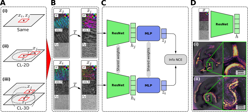
Figure 4: Illustration of the proposed 3D context contrastive learning scheme. (A) Correlated views of similar nerve fiber architecture are sampled as positive pairs of image patches $(x_{i},x_{j})$ as (i) identical patch pairs (Same), (ii) as in-plane shifted patches within a radius $r$ (CL-2D), or (iii) around a sphere with radius $r$ in proximity to the anchor example across sections using nearest neighbor interpolation (CL-3D). (B) Data augmentations $T$ for 3D-PLI are randomly applied to sampled patches to promote learning representations that are robust to typical variations in 3D-PLI measurements. Patches are visualized as transmittance $I_{T}$, retardation $|\sin\delta|$ and the fiber orientation map (FOM) in HSV color space (hue: direction $\varphi$; saturation, brightness: inclination $\alpha$). (C) The contrastive learning framework [Chen et al., 2020] consisting of a ResNet encoder, hidden features $h_{i}$ and $h_{j}$, a fully connected MLP projection head, projections $z_{i}$ and $z_{j}$ and InfoNCE loss. (D) For inference, the trained encoder is applied on un-augmented patches $x$ to extract 3D-PLI texture features $h$. Whole sections are converted to feature maps using a sliding window approach. Two example feature maps are shown on top of transmittance maps for reference highlighting (i) U-fibers and (ii) primary visual cortex (V1).

Contrastive learning aims to learn robust and descriptive representations of data samples by contrasting similar and dissimilar pairs of samples. The goal is to learn an encoding function $f$ which groups similar samples closely together in representation space while pushing dissimilar samples apart from each other. Assuming a reasonable measure of similarity that can be efficiently derived from the data, similar samples are generated as positive pairs consisting of an anchor sample and a positive sample with high similarity, while for negative pairs the anchor is combined with a dissimilar negative sample.

In this study, we derive similarity from the spatial neighborhood of image patches in a 3D-Context Contrastive Learning objective. Given a random location $p^{a}$ for the anchor sample, we generate a positive sample from neighborhood locations $p^{+}=p^{a}+\Delta p$, where $\Delta p$ is chosen based on two variants of spatial similarity (Fig. 4A):

1. CL-2D, where we sample $\Delta p$ on an in-plane circle with radius $r$ from the same tissue section. We regard Same as a special case of CL-2D, where $r$ = 0.

2. CL-3D, where we sample $\Delta p$ on a sphere with radius $r$ across sections, and choose the cross-section location for $p^{+}$ by rounding the sampled coordinate to the nearest available section, but exclude the section from which the anchor sample was taken (i.e. $p^{a}$ and $p^{+}$ are always located on different sections). For $r$ = 0 µm, we sample at the same in-plane coordinates but from a random adjacent section.

For $p^{a}$, only locations with visible tissue are considered to avoid sampling positive pairs containing background only, using the segmentation masks obtained in Sec. 2.3. In addition to the spatial sampling, we perform random augmentations for all samples as detailed in Sec. 2.2 (Fig. 4B).

For training encoder $f$, we build on the SimCLR contrastive learning framework [Chen et al., 2020] (Fig. 4C). In this specific framework, $N$ augmented positive pairs $(\tilde{x}_{i},\tilde{x}_{j})$ are sampled for each training step and stored in minibatches of $2N$ total examples $\{\tilde{x}_{k}\}$. We refer to the set containing indices $(i,j)$ for all $N$ positive pairs in the minibatch as $\Omega$. For each positive pair, all $2(N-1)$ other samples $\{\tilde{x}_{k}\}_{k\neq i,j}$ are considered negative samples. Encoder $f$ typically refers to a deep learning model, which yields network activation vectors $h_{k}=f(\tilde{x}_{k})$ as representations. An additional projection head $g$ is introduced to map the activations $h_{k}$ to a lower dimensional space of projections $z_{k}=g(h_{k})$, on which contrastive loss is applied. The training objective is given in terms of the InfoNCE loss [van den Oord et al., 2018]:

$$\ell_{i,j}=-\log\dfrac{\exp({\operatorname{S_{c}}(z_{i},z_{j})/\tau})}{\sum_{k=1}^{2N}\mathds{1}_{[k\neq i]}\exp({\operatorname{S_{c}}(z_{i},z_{k})/\tau})},$$ (15)

where $z_{k}=g(f(\tilde{x}_{k}))$ and similarity metric $\operatorname{S_{c}}$ chosen as the cosine similarity with temperature parameter $\tau$. The former per-sample loss is accumulated into a total loss as

$$\mathcal{L}=\frac{1}{2N}\sum_{(i,j)\in\Omega}\ell_{i,j}+\ell_{j,i}.$$ (16)

After training, the projection head is discarded and for inference only representations $h=f(x)$ on un-augmented samples $x$ are used (Fig. 4D).

2.5 Model training

Model Architecture.

For the encoder $f$ we use a ResNet-50 [He et al., 2016] model with 3 input channels and remove the last fully-connected layer. We reduce the number of features for all blocks in the ResNet-50 architecture to 1/8 to limit the encoder capacity, which results in 256-dimensional hidden representations. Training models with the full ResNet-50 capacity systematically resulted in high activations to infrequent but highly pronounced structures such as tangential cut radial fibers. Such structures made it trivial to solve the contrastive learning objectivate based on spatial similarity. Reducing the model capacity prevented the model from overfitting to these specific structures and let us learn more general concepts of fiber architecture. For projection head $g$ we use a two-layer MLP with ReLU activations, hidden feature size of 90 and outputs $z$ of size 32. To feed 3D-PLI images to the ResNet, parameter maps transmittance $I_{T}$, direction $\varphi$ and retardation $|\sin\delta|$ are stacked as $x$ = ($I_{T}$, $\sin\delta\cdot\cos(2\varphi)$, $\sin\delta\cdot\sin(2\varphi)$) to the channel dimension, which resolves the cyclic nature of direction values $\varphi$. We standardize the input channels by running mean and standard deviation over the first 1 024 batches during training.

Implementation.

We use PyTorch [Paszke et al., 2019], PyTorch Lightning [Borovec et al., 2022], and Hydra [Yadan, 2019] frameworks using the Quicksetup-ai [Mekki et al., 2022] template for building our model. Data augmentations (cf. Sec. 2.2) are implemented using the Albumentations [Buslaev et al., 2020] framework. Training is conducted using a distributed data-parallel strategy on 4 Nvidia A100 GPUs with synchronized batch normalization statistics [Ioffe and Szegedy, 2015] on the supercomputer JURECA-DC at the Jülich Supercomputing Centre (JSC) [Thörnig, 2021].

Data sampling.

We sample square patches of size 192 pixels (250 µm) as anchor examples from random locations within the training volume, excluding background using the previously generated cortex segmentation. For each anchor example, we sample positive examples from a location in spatial proximity, depending on the chosen definition of spatial similarity. As we sample patch locations on the fly, we do not have a fixed dataset size but define an epoch as the sampling of 512 $\times$ 512 = 262 144 positive pairs. Per training step, we sample 512 anchor examples and positive examples and process them evenly split on the 4 GPUs.

Data augmentation.

In all examples, we apply an affine transformation (scaling from [0.9, 1.3] on each axis, rotation from [-180°, 180°], and shearing from [-20°, 20°] on each axis) with linear interpolation and subsequent center cropping to crops of size 128 pixels (166 µm) to eliminate padding effects. Subsequently, we perform random flipping on the center crops and scale relative thickness $t$ (Eq. 4) and the attenuation coefficient $\mu$ (Eq. 3) each by random scaling from a logarithmic distribution with basis 2 from [-1, 1]. As the last augmentation, we perform Gaussian blur with $\sigma$ from [0.0, 2.0] with a probability of 50%.

Training.

All augmented crops are fed to the encoder model and projection head in order to minimize the loss in Eq. 16. We use Adam optimizer [Kingma and Ba, 2017] with a learning rate of 10^-3, a weight decay of 10^-6 and default parameters $\beta_{1}$ = 0.9, $\beta_{2}$ = 0.999 and $\epsilon$ = 10^-8. For the choice of temperature parameter $\tau$ in Eq. 15 we follow the optimal choice of $\tau$ = 0.5 reported by [Chen et al., 2020] when training until convergence. We apply the same loss for training and validation. All models are trained until convergence if the validation loss did not reduce for more than 50 epochs, which took between 195 (2D context) and 400 (3D context) epochs.

Inference.

After training, model weights are frozen and inference is performed on complete sections using the trained ResNet encoder, discarding the projection head. Each section is converted into feature maps using a sliding window approach by dividing 3D-PLI parameter maps into tiles of size 128 pixels (166 µm) with 50% overlap. The overlap is chosen to better represent pixels at the edges of patches that would otherwise lie on the boundary between adjacent patches. We extract a 256-dimensional feature vector for each tile without applying the data augmentation used in training. All extracted feature vectors are then reassembled into whole feature maps with a reduced in-plane resolution of 84.4 µm per pixel compared to the original input parameter maps, but 256 characteristic feature channels describing for the local texture content. Compared to the section thickness of 60 µm, this makes the feature voxels approximately isotropic.

2.6 GLCM texture feature baseline

The present approach enables learning of texture features specifically for 3D-PLI parameter maps. As a baseline for texture analysis, we use Grey-Level Co-occurrence Matrices (GLCM) [Haralick et al., 1973] as a well-established approach to represent textures using higher-order statistics in medical imaging such as CT, MR, and PET [Scalco and Rizzo, 2017]. Using the same sliding window approach introduced in Sec. 2.5, we divide 3D-PLI parameter maps into tiles of size 128 pixels (166 µm) with 50 % overlap and compute GLCMs for each of them.

Direction maps $\varphi$ represent the absolute orientation of fibers within the imaging plane. Since we want to find texture representations that are independent of their absolute orientation, we are more interested in local patterns of $\varphi$ than in their absolute values. We use the Sobel operator as a first derivative filter to highlight image edges and eliminate absolute values of $\varphi$. To filter direction values $\varphi$, we need to resolve their circular nature. Therefore, we represent direction angles $\varphi$ in polar form as complex number

$$z=\cos(2\varphi)+i\sin(2\varphi)$$ (17)

and apply Sobel filtering as

$$G_{x}=K_{x}*z\hskip 8.53581pt\text{and}\hskip 8.53581ptG_{y}=K_{y}*z$$ (18)

with convolution operator $*$ and Sobel filter kernels $K_{x}$ and $K_{y}$. We aggregate the filtered images as

$$\hat{\varphi}=|G_{x}+G_{y}|/12,$$ (19)

where $|.|$ extracts the magnitude of complex numbers, and dividing by 12 normalizes the filtered values to [0, 1].

We compute normalized and symmetric GLCMs for 32 equally spaced bins of parameters maps $I_{T}$, $\sin\delta$ and $\hat{\varphi}$ for distances [1, 2, 4] and angles [0, $\pi$/4, $\pi$/2, 3$\pi$/4]. From each GLCM, we compute contrast, correlation, energy, and homogeneity as features [Haralick et al., 1973]. We concatenate the features for all parameter maps and distances while averaging over the angles to make the features robust to rotations. Each feature is then standardized by its global mean and standard deviation. In this way, we obtain a baseline feature vector of length 36, which we can compare to the learned deep texture representations of dimension 256.

3 Experiments and Results

We train CL-2D and CL-3D models using the data from the occipital lobe of a vervet monkey brain described in Sec. 2.1. We split the volume into sections for training (#962 - #1077), sections for validation (#1078 - #1083), and sections for testing (#851 - #961) as shown in Fig. 2A. We evaluate the feature representations produced by the models regarding their interpretability, spatial consistency, and applicability for downstream tasks. In particular, we compare the extent to which features of different approaches can be related to brain morphology and their robustness to variations between sections. We investigate the main factors of variation specifically for the CL-3D features and demonstrate that they lend themselves to interactive data exploration and identification of nerve fiber architecture in large volumes of 3D-PLI data. All experiments are based exclusively on features extracted from the test data sections.

3.1 Main factors of variation in the learned representations

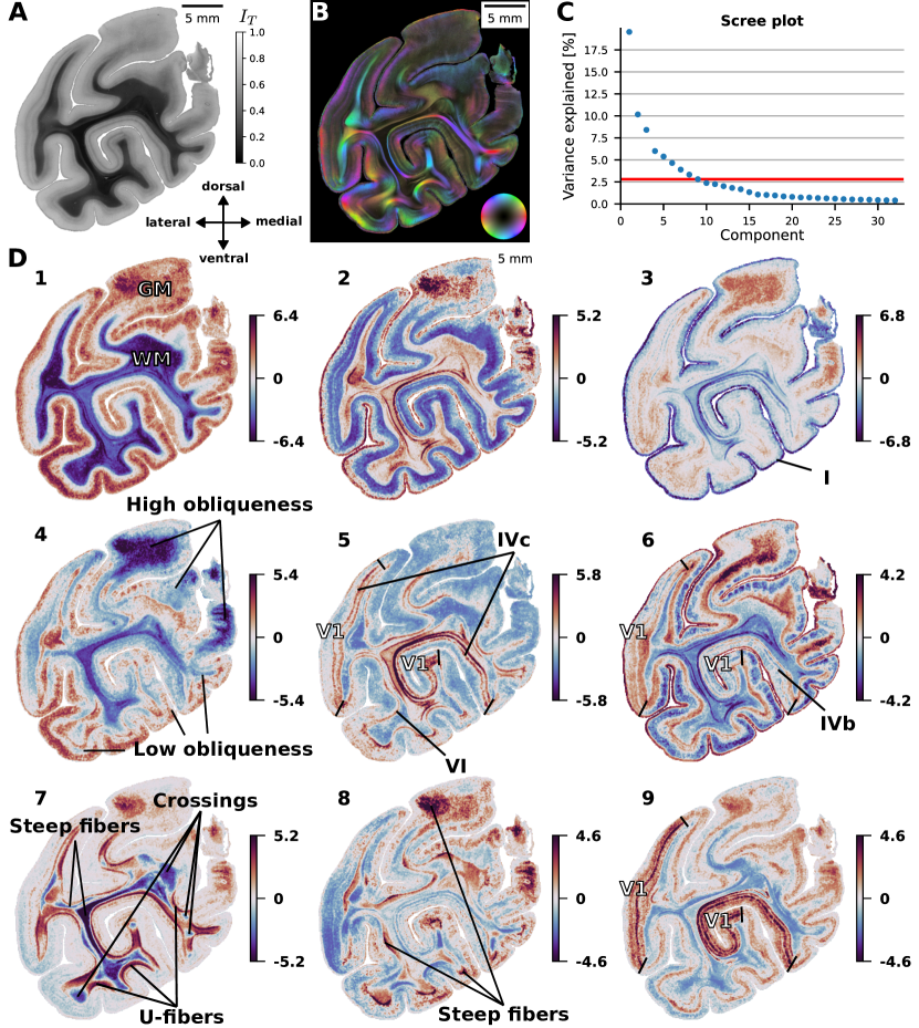
Figure 5: Projection of the CL-3D texture representations from section 961 onto the 9 PCA components with largest explained variance. (A) Transmittance and (B) fiber orientation maps (FOM) for the section. (C) Scree plot showing the variance explained by the first 32 components. The horizontal red line indicates the variance explained by the 9th component of 2.8%. (D) Color-coded parameter maps of the selected PCA components, with background pixels masked as zero. The maps reveal anatomically plausible structures. GM: gray matter, WM: white matter, V1: primary visual cortex.

To gain insights into the main factors of variation captured by the CL-3D features, we perform principal component analysis (PCA) on a random subset of 1 million pixels from the feature maps. We use the estimated principal axes to project the feature channels for the entire dataset onto the 9 components with the largest explained variance (64.2% cumulative explained variance), with at least 2.8% of variance explained per component.

Fig. 5D shows images of the first 9 principal components, which in general terms reveal anatomically plausible structures. Component (1) shows a clear separation of white matter (WM) and gray matter (GM). Within GM, higher values indicate layers with a lower density of radial fibers. Within GM, values in component (2) distinguish between layers with high density of radial fibers (low values) and high density of tangential fibers (high values in the superficial layers, which contain mainly tangential fibers, and values around 0 in the Gennari stripe, which presents both radial and tangential fibers), while high values within WM highlight edges between fiber bundles. Low values in component (3) highlight layer I, which contains a high density of tangential fibers, as well as WM structures with high fiber density that run in-plane, such as the Tapetum. High values indicate tangentially sectioned radial fibers. Component (4) has low values towards out-of-plane fibers and highly oblique cortex and high values towards superficial GM layers with a low density of radial fibers and low obliqueness. Component (5) shows high values for layer IVc in the primary visual area (V1) and layer VI throughout the whole cortex. In component (6), high values show layer I throughout the cortex as well as layer IVb within V1 (Stria of Gennari), i.e., they highlight GM layers with a high density of tangential fibers. High and low values in (7) mainly represent WM, with high values indicating U-fibers and other in-plane fibers and low values indicating steep fibers or crossings. The stratum sagittale (SS) has the lowest values, as here fibers emerge vertically from the plane. High values in GM mainly highlight tangentially sectioned radial fibers. High values in (8) also highlight tangentially sectioned radial fibers in GM. Additionally, they indicate abrupt twisting of flat, in-plane fibers that twist out of plane at the GM/WM transition and show parts of U-fibers that are cut through the plane. In component (9), layers IVa, IVc and VI within V1 are characterized by high values.

3.2 Linear relationships of learned features to brain morphology

Table 1: Proportion of variance in the morphological measures cortical depth, white matter depth, curvature, and obliqueness that can be explained by a linear model from extracted features. We consider features by contrastive learning methods using cross-section pairs (CL-3D) and in-plane pairs (CL-2D) compared to GLCM texture features. The goodness of the fit is calculated using the coefficient of determination $R^{2}$. A medium sampling radius of $r$ = 118 µm in CL-3D has the overall highest relationship to the morphological measures.

Method	$r$ [ µm ]	Cortical depth	White matter depth	Curvature	Obliqueness
GLCM	-	0.57	0.23	0.03	-0.02
CL-2D	0	0.59	0.16	0.01	0.14
	118	0.80	0.29	-0.02	0.32
	236	0.78	0.19	-0.03	0.33
CL-3D	0	0.80	0.31	0.04	0.47
	118	0.81	0.36	0.02	0.50
	236	0.81	0.32	0.02	0.45

(a) CL-3D texture features

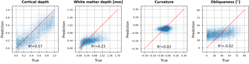
(b) GLCM texture features

Figure 6: Proportion of variance for different morphological parameters explained by (a) the proposed CL-3D feature representations and (b) GLCM texture features. A linear model was trained via least squares to predict cortical depth, white matter depth, curvature, and obliqueness. Predicted and true target measures are shown as blue scatter plots, where red lines indicate an optimal fit. Goodness of fit is calculated by the coefficient of determination $R^{2}$.

Fiber architecture has mutual dependencies with cortical morphology [Van Essen, 1997, Striedter et al., 2015]. To investigate to what extent different texture representations are related to cortical morphology, we extract a range of morphological parameters from our test data. In particular, based on the cortex segmentation described in Sec. 2.3, we compute a Laplacian field between outer pial and inner white matter surfaces using the HighRes cortex [Leprince et al., 2015] module included in brainvisa [Cointepas et al., 2001]. We extract the following measures:

• Equivolumetric cortical depth [Bok, 1929] as the depth along cortical traverses following the gradient of the Laplacian field, compensating for the effect of cortical curvature through the divergence of the same field. It has values of 0 at the Pial and 1 at the gray-white matter surface.

• White matter depth defined as the shortest distance from each voxel within white matter to the interface between the cortical ribbon and white matter in millimeters.

• Cortical curvature as the divergence of the gradient of the Laplace field between Pial and white matter surfaces ([Goldman, 2005], Equation 3.8; [Leprince et al., 2015])

• Obliqueness of the sectioning plane, computed as the absolute angle between the gradient of the Laplacian field and the sectioning plane with values in [0°, 90°].

White matter depth allows us to investigate to what extent the texture features can differentiate between superficial fiber bundles such as U-fibers in contrast to deeper bundles. The relative cutting angle, while not a morphological measure, provides an important geometric parameter affecting the 3D-PLI textures.

We follow the approach of [Spitzer, 2020] and investigate how well a linear model can predict these measures from the learned feature representations. We randomly select 10 000 voxels from the training set, and compute both their feature representations using the trained models as well as the above-mentioned morphological measures. The features are standardized using Z-score normalization and used to fit a linear regression model via least-squares. The goodness of the linear fit is then determined by calculating the coefficient of determination $R^{2}$, which denotes the proportion of variation in the measures that can be explained by the feature representations. We compute $R^{2}$ for predicted values from 10 000 randomly selected voxels from the test set.

Scatter plots in Fig. 6 summarize the results for predicted and true values. We observe a strong linear relationship of the proposed CL-3D features to cortical depth ($R^{2}$ = 0.81), a moderate relationship to obliqueness ($R^{2}$ = 0.50) and white matter depth ($R^{2}$ = 0.36), and no significant correlation with curvature ($R^{2}$ = 0.02). For obliqueness, especially larger angles can be predicted from the CL-3D features, while smaller angles do not show a good fit in the scatter plot. The relative ranking of variance explained by GLCM texture features in cortical depth ($R^{2}$ = 0.57), white matter depth ($R^{2}$ = 0.23), and curvature ($R^{2}$ = 0.03) is identical, but values are overall lower. In contrast to CL-3D features, the GLCM texture features are not related to obliqueness ($R^{2}$ = -0.02). In comparison to CL-2D in Tab. 1, CL-3D has an overall higher relationship to the morphological measures. A medium sampling radius of $r$ = 118 µm improves the relationship for both methods over a larger radius ($r$ = 236 µm) or sampling from the same in-plane coordinates ($r$ = 0 µm).

3.3 Clustering of learned features

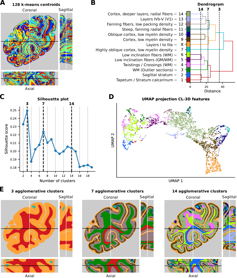
Figure 7: Agglomerative hierarchical clustering of 128 k-means centroids shows a hierarchy of fiber architecture. (A) The 128 k-means centroids form superpixel-like clusters. (B) Dendrogram representing distances between identified clusters before merging and approximate labels naming the structures with highest overlap with each cluster. (C) Silhouette plot showing local maxima around 3, 7 and 14 clusters. (D) UMAP projection of the CL-3D features. The color of each point corresponds to the respective cluster assignment. (E) Clustering results for 3, 7 and 14 clusters.

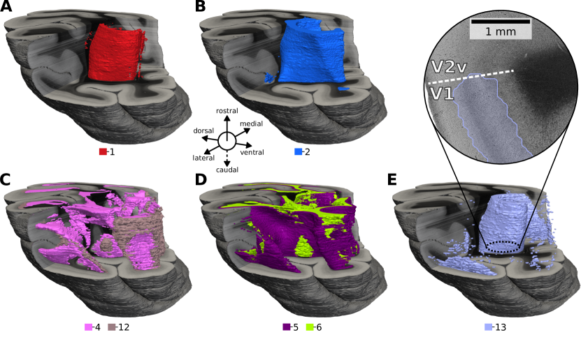
Figure 8: Hierarchical agglomerative clustering of representations extracted by the CL-3D approach produces consistent 3D segments with anatomical relevance. (A) Approximately the Tapetum and stratum calcarinum (1). (B) Contains steep fibers of the sagittal stratum (2). (C) Close to in-plane twisting or crossing fibers (4) and flat fanning fibers (12). (D) Flat fibers for layer VI (5) and WM (6). (E) Mainly layers IVb-V of primary visual area (V1), sometimes including layer VI (13). It is less clearly defined than other clusters.

3.3.1 Hierarchical clustering

We perform hierarchical cluster analysis in the embedding space of the learned CL-3D features to evaluate how far the features form maps of characteristic nerve fiber configurations. Hierarchical clustering creates a tree-like structure of hierarchical relationships among data points as a dendrogram based on their similarity in representational space. We choose the bottom-up approach for agglomerative clustering, which merges closest clusters based on our choice of Euclidean distance and Ward linkage. To reduce noise and computational effort, we cluster the PCA-reduced feature maps from Sec. 3.1, but with 20 components as channels and 80.4% total explained variance. To increase the receptive field and reduce in-plane noise, each feature map is smoothed by an in-plane 2D Gaussian kernel with a standard deviation of $\sigma=1$ which provides a good trade-off between noise and sensitivity to smaller structures.

We select features from foreground voxels across all test sections. Due to the huge amount of 16 million data points, hierarchical clustering cannot be applied directly to the data points. Instead, we perform a two-step approach by first performing k-means clustering on a subsample of 100 000 features using $k=128$. We use the 128 resulting cluster centers to assign all remaining 15.9M data points to these clusters, allowing us to represent the whole test volume by superpixel-like clusters (Fig. 7). As a second step, we perform agglomerative hierarchical clustering to obtain a cluster dendrogram (Fig. 7B). We compute silhouette scores for the clustering results at different distance thresholds to determine the most distinct clusterings for visualization (Fig. 7C).

While score values are overall declining, we can identify local maxima around 3, 7, and 14 clusters. Results for these optimal cluster configurations are summarized in Fig. 7E. A range of characteristic aspects of fiber architecture is revealed: Solutions for 3 clusters demonstrate a first global differentiation of the data into GM and WM. Due to its high fiber density, cortical layer VI is sometimes represented inside the WM cluster. We further observe a small cluster of tangentially cut cortex.

The configuration with 7 clusters differentiates superficial and deep cortical layers. This segregation is shaped by the packing density of radial fibers in the deeper layers, and the tangentially running fibers close to the pial surface. For WM, voxels are split into two clusters: 1) the red cluster in Fig. 7E highlights densely packed fibers with out-of-plane orientation of the sagittal stratum (SS), as well as surrounding densely packed in-plane fibers of the tapetum. 2) the green cluster in Fig. 7E encompasses in-plane fibers or fibers with relatively low inclination, together with steep but less densely packed fiber bundles.

The configuration of 14 clusters reveals an increased sensitivity to specific WM fiber bundles and displays a cortical region delineation for the primary visual cortex (V1). Furthermore, a range of fiber architectural properties can be recognized in the maps corresponding to the clusters in Fig. 7B:

• Cluster (1) shows the Tapetum and stratum calcarinum (SC), characterized by approximate in-plane fibers with high packing density.

• Cluster (2) displays densely packed, highly inclined fibers and fibers of the sagittal stratum (SS) with out-of-plane orientation.

• Cluster (3) includes WM voxels from sections with an artifact-related increased light transmittance (not present in the section shown in Fig. 6E).

• Cluster (4) mainly displays WM voxels, but in some cortical segments also encompasses layer VI. WM covered by these voxels is characterized by fibers with high packing density, small inclination angles, and twisting or crossing patterns.

• Cluster (5) mainly highlights layer VI of cortical segments complementing cluster 4. WM voxels encompass fibers with low packing density and low inclination at the border between GM/WM.

• Cluster (6) reveals only WM voxels with very small fiber inclination mostly parallel configurations, with only a few crossings.

• Cluster (7) highlights voxels located in highly oblique cortex with layers characterized by low myelination. When not tangentially sectioned, this portion of the cortex is encompassed by cluster (9).

• Cluster (8) highlights the most superficially located bands of tangential fibers, namely those of the zonal layer and the Kaes–Bechterew stripe, which are located in cytoarchitectonic layers I and IIIa, respectively [Zilles et al., 2015], and found throughout the whole cortex.

• Cluster (9) covers cortical layers with low density of myelin. The width of this cluster varies along the cortical ribbon. Some areas, where radial fibers reach almost up to layer II, are characterized by a narrow band of cluster (9), while in other areas it is broad because their radial fibers only reach into layer IIIb. The cluster disappears in the cortex of highly compressed sulci.

• Voxels in cluster (10) are also located in obliquely sectioned layers with a low myelination while being less oblique than those of cluster (7).

• Cluster (11) encompasses steep radial fibers fanning out at the apex of the gyrus.

• Cluster (12) highlights approximate in-plane fibers with low packing density, fanning out at the apex of the gyrus.

• Voxels of cluster (13) are restricted to the primary visual area (V1). They are mainly found in layers IVb-V, but, depending on packing density, sometimes also those of layer VI). This cluster could reflect local cortical connectivity within V1.

• Cluster (14) highlights deeper layers mainly due to their density of radial fibers. Its width varies along the cortical ribbon and is inversely related to the width of cluster (9). In V1 cluster (14) is restricted to layers IIIb and IVa. In the remaining cortex, depending on the area it can reach from layer IIIa or IIIb to layer V or VI.

To visualize the organization of data points in the learned representational space, we additionally perform UMAP [McInnes et al., 2020] projection of the PCA-reduced features used for clustering on two dimensions using 4 000 example data points. The projections in Fig. 7D show an organization of the features in a continuous band along cortical depth starting from superficial layers (clusters 8 and 9), to deeper layers (clusters 13, 14, 5, and partially 4) until reaching WM clusters (3, 6 and partially 4). Branches to the sides highlight different degrees of obliqueness of cortical layers (i.e. clusters 7, 9, and 10). Clusters for structures such as the SS (cluster 2), Tapetum/SC (cluster 1), or layers of V1 (cluster 13) form separate branches in the projected space.

3.3.2 Consistency of clusters across sections

In addition to the 2D cluster maps, we assemble 3D renderings of the configuration with 14 clusters (Fig. 8). Although the feature representations for CL-3D were only generated based on in-plane texture information without cross-section constraints, the volume rendering reveals consistent cluster boundaries across sections, as can be observed by the smooth cluster shapes in the cross-sections. Cluster 13 stands out in being more noisy than other clusters.

To better quantify the cross-section consistency of feature clusters, we compute the intersection over union (IoU) of cluster assignments between adjacent sections for different numbers of clusters assigned to the feature maps by k-means (2, 8, 32 and 128 clusters). Since the absolute coordinates are not encoded in feature space, this analysis provides us insights into the robustness of representations to inter-section variations arising from histological processing.

Table 2: Cross-section consistency as mean IoU of cluster assignments between neighboring sections based on different representations. Contrastive learning approaches by different sampling strategies for positive examples (same: CL, in-plane: CL-2D, cross-section: CL-3D) are compared to baseline GLCM texture features. Using a cross-section sampling strategy in CL-3D achieves overall highest consistency.

Method	$r$ [ µm ]	2 clusters	8 clusters	32 clusters	128 clusters
GLCM	-	95.2	58.4	34.1	19.4
CL-2D	0	88.9	47.1	25.0	12.8
	118	95.4	61.2	35.9	20.0
	236	95.0	55.8	36.7	21.0
CL-3D	0	89.2	70.8	50.2	30.3
	118	96.1	70.5	51.0	32.3
	236	95.4	71.9	50.7	32.0

The IoU scores are reported in Tab. 2, and are overall declining with increasing number of clusters. Cluster assignments based on CL-3D feature representations are more consistent across different numbers of clusters than the other methods. By using the same image as the anchor and positive examples in CL, IoU values fall below the GLCM baseline. Using an in-plane context in CL-2D results in IoU scores comparable to the GLCM baseline.

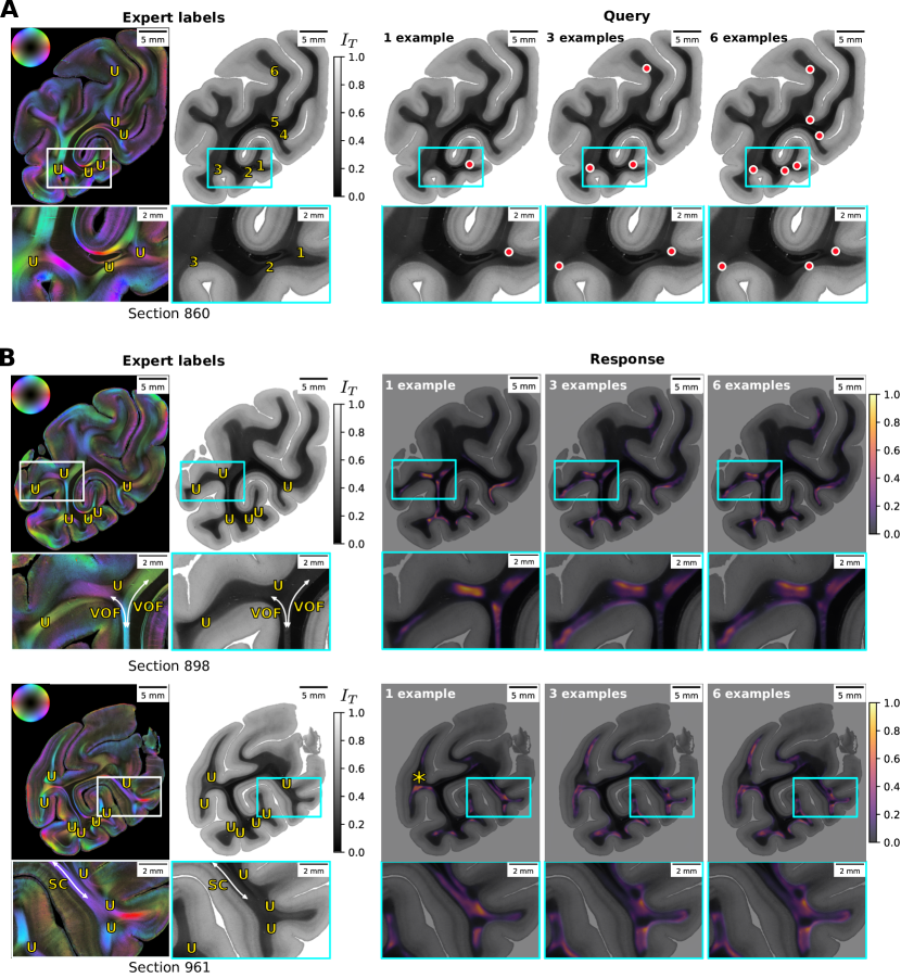
Figure 9: The proposed CL-3D feature representations allow for retrieval of distinct nerve fiber patterns by presenting prototypical image patches as a query and searching for closeby patches in the feature embedding space. (A) A section from the test set used to place query points that identify positive examples for U-fibers. Yellow ’U’ markers in the fiber orientation maps (and numbers in the same positions in the corresponding transmittance images) show U-fibers identified by an expert [Takemura et al., 2020]. Red dots highlight query points used to identify U-fibers with increasing amounts of examples (namely 1, 3, and 6). Responses to the queries are shown in (B) for two other sections from the test set. They show the similarity for all data points to the mean representation of example points as affinity maps from voxels in the feature maps. Asterisk highlights the position of a U-fiber not detected by this procedure. U: U-fibers, VOF: vertical occipital fascicle, SC: stratum calcarinum.

3.4 Using learned features for retrieval of common fiber orientation patterns

The proposed method embeds image patches with similar fiber architectural properties as close points in the learned feature space. Therefore, we expect that the resulting feature representations can be used for retrieval of similar structures, given a known "prototype" image patch. To evaluate the suitability for such an application, we investigate how far U-fiber structures can be found in 3D-PLI image data from a few image examples. Although U-fibers are represented by one of the principal axes (Fig. 5D (7)), they do not appear as individual clusters in Fig. 7E. To demonstrate that the representations can still be used to identify specific nerve fiber architectures, we provide a few positive examples of U-fiber systems to perform a query for similar fiber configurations (Fig. 9).

Unfortunately, access to detailed, annotated data in combination with 3D-PLI measurements is limited, as reliable identification of positive and negative examples is not always possible. However, we can still search for U-fibers by selecting only a few positive examples that could be identified with confidence from 3D-PLI images in [Takemura et al., 2020]. For this purpose, we select up to 6 query points as positive examples (Fig. 9A) and compute affinity maps that show the similarity of all voxels in the feature maps to the averaged query features in representational space as responses. For this experiment, we smooth PCA-reduced feature maps with 20 components (80.4% total explained variance) by a 2D Gaussian kernel analog to Sec. 3.3, but set $\sigma$=2 to increase the receptive field of texture features. This allows to represent texture for larger structures such as U-fibers and improves retrieval results. We calculate the affinity between feature points using a Gaussian radial basis function (RBF) kernel with $\sigma$ = 3.5.

The affinity maps reveal peak regions at locations displaying U-fiber structures (Fig. 9B). They activate to all U-fibers identified by an expert, except for one missing activation for a U-fiber, highlighted by the asterisk. In addition, the activations highlight some fiber bundles that are not labeled as U-fibers, such as the vertical occipital fascicle (VOF) or the stratum calcarinum (SC). Although the false positive activations for VOF and SC could be suppressed through more query points, they do not disappear completely.

4 Discussion

4.1 Feature representations encode fundamental aspects of fiber architecture

The feature representations extracted by the proposed CL-3D method from 3D-PLI image patches encode distinct aspects of fiber architecture. Our experiments in Sec. 3.3 have shown that the features form hierarchical clusters that represent gray and white matter, myeloarchitectonic layer structures, fiber bundles, fiber crossings, and fiber fannings. These clusters are spatially consistent and often highlight specific characteristics of fiber architecture as locally connected structures (Fig. 7). Even without explicit clustering, the main PCA components of the feature embedding space produce maps that highlight fundamental principles of fiber architecture (Fig. 5). This indicates that proximity of features in the embedding space, which is efficient and easy to compute, serves as a suitable proxy measure for similarity of fiber architecture as captured in the corresponding image patches. This is in contrast to directly measuring similarity of 3D-PLI image patches, where strong differences can occur despite very similar fiber configurations. Thus, the CL-3D features are well suited to facilitate downstream applications for 3D-PLI image analysis.

4.2 Feature representations are robust to common variations in histological processing

While encoding relevant aspects of fiber architecture, the proposed CL-3D features proved to be robust against many other sources of texture variation. We were able to observe this robustness in the 3D stacking of consecutive images with derived cluster segments from CL-3D features. The segments showed a very high overlap across brain sections (Tab. 2), in particular, compared to the clustering of statistical GLCM features as a baseline, but also w.r.t. CL-2D features which only learned from in-plane context. The volume renderings in Fig. 8 illustrated the consistency of clustering CL-3D features as spatially consistent 3D segments. This suggests that CL-3D promotes the learning of representations that are more robust to discrepancies between independently processed sections.

CL-3D features were also found to be robust to the absolute in-plane orientation of texture, as shown by consistent laminar patterns of cluster assignments regardless of their absolute orientation in 2D (Fig. 7). We attribute this to the random affine transformation and flipping used for data augmentation, which prevent the encoder from encoding the absolute orientation of texture as a descriptive feature.

At the same time, CL-3D features showed sensitivity to the relative cutting angle of cortical voxels, which we observed as a correlation with the independently measured obliqueness of image patches (Tab. 1). Obliqueness is a local feature of histological images that is consistent across adjacent sections and could be exploited by the contrastive learning objective to identify closeby positive pairs. For the majority of cortical voxels, however, this effect on the features seems to be small. Only for very high obliqueness the CL-3D features formed some smaller branches in the UMAP projection in Fig. 7D or isolated clusters in Fig. 7E. This is consistent with the observation from the scatter plots (Fig. 6(a)) that the CL-3D features are only related to obliqueness for larger angles, being unable to predict variation in smaller angles. If the representation of obliqueness in downstream applications is nevertheless not intended, a supervisory signal that combines texture patches with different cutting angles into the same label could be helpful. For unsupervised learning, treating obliqueness as a confounding variable [Snoek et al., 2019, Dinga et al., 2020] could also help to reduce its effect.

4.3 Retrieval and mapping as possible downstream applications

Fiber architecture is expressed in highly complex textures when measured at microscopic resolution. This makes it extremely challenging to navigate and explore larger stacks of 3D-PLI images. An obvious, albeit simple, application is the search for similar local configurations of nerve fibers, given a template image patch used as a prototype for such a query. We took a search for U-fiber structures as an example (Fig. 9), where independent expert annotations could be obtained from a previous study, and were able to demonstrate the feasibility of such a retrieval task with the proposed CL-3D features.

We showed that features cluster into groups that follow certain fiber bundles such as the sagittal stratum or the Tapetum (Fig. 7). While this might at first suggest to use the features for automated brain mapping tasks, the clusters did not lend themselves to a sufficiently accurate delineation of anatomical structures. This could be due to partial volume effects of patches used to represent texture, or to the smoothing performed before clustering to denoise the features. As contrastive learning focuses on the most characteristic properties of texture to identify positive pairs, some aspects of fiber architecture might overshadow others. The clustering in Fig. 7E, for example, did not fall into accurate GM/WM segments. This could be due to features reflecting the density of myelinated fibers more than other aspects of fiber architecture, thus including the deepest cortical layers in the WM segment, where the density of myelinated fibers is still very high. Since the degree of sharpness of the boundary between cortex and white matter constitutes a criterium for the identification of architectonically distinct areas (e.g., REF [Niu et al., 2020]), another explanation would therefore be that brain areas with a blurry boundary are those in which voxels of layer VI merge into the WM segment. It should be noted though, that the proposed method is not specifically designed for performing automatic brain mapping. A supervised approach for brain mapping as a downstream application can nevertheless be promising with the proposed features. A more systematic investigation into fiber architectonic mapping based on CL-3D features will thus be an important follow-up work of this study.

4.4 Relationship of feature representations with cortical morphology

Cortical layers are arranged along the cortical depth and have distinct characteristic architectures. Being able to regress cortical depth from texture features therefore suggests that they encode information about the layering structure of the cortex. The high amount of variance in cortical depth explained by the CL-3D and CL-2D features (Tab. 1) indicates that these models have indeed learned to represent layer-related textures. For CL-2D, this claim is also supported by the observation that the main PCA components highlight layers (Fig. 5) and that the features fall into layer-related clusters (Fig. 7). Compared to the relationship between GLCM features and cortical depth, deep texture features by CL-3D and CL-2D show a higher relation with cortical depth, suggesting that contrastive learning can represent cortical architecture better than the GLCM baseline. Furthermore, being able to regress the distance of the centers of image patches to the cortical ribbon (Tab. 1) suggests that the CL-3D features separate deep from superficial fiber bundles such as U-fibers [Decramer et al., 2018, Shinohara et al., 2020].

Methods for analyzing the laminar structure of the cortex typically require representations that are robust to cortical folding [Schleicher et al., 1999, Waehnert et al., 2014, Leprince et al., 2015]. While the CL-3D model learned to represent some curvature-related patterns such as for fanning radial fibers at gyral crowns (Fig. 7), correlation with curvature was very low overall (Tab. 1), indicating moderate robustness of the proposed feature representations to cortical folding. For CL-3D and CL-2D, the low relationship might be attributed to the affine transformation applied in the contrastive learning setup, which performs scaling and shearing operations on the texture examples. It should be noted that in addition to the curvature definition used in Sec. 3.2, other established definitions [Goldman, 2005] that have not been considered in this study might lead to different results.

5 Conclusion and Outlook

Aiming to improve automatic mapping and analysis of fiber orientation distributions in the brain, we introduced a self-supervised contrastive learning scheme for extracting "deep" feature representations for 3D-PLI image patches at micrometer resolution. We specifically proposed 3D context Contrastive Learning (CL-3D), where positive pairs are sampled based on their spatial proximity across nearby brain sections. Without any anatomical prior information given during training, the feature representations extracted by CL-3D were shown to highlight fundamental patterns of fiber architecture in both gray and white matter, such as myelinated radial and tangential fibers within the cortex, fiber bundles, crossings, and fannings. At the same time, feature representations by CL-3D proved to be more robust to variations between independently measured sections, such as artifacts arising from histological processing, compared to statistical methods and representations by in-plane sampling of positive pairs in contrastive learning (CL-2D).

The present study opens new perspectives for automated analysis of fiber architecture in 3D-PLI. Due to the low-dimensional embedding space, the feature representations can aid in interpretation of 3D-PLI textures and improve computational efficiency of downstream 3D-PLI analysis. For example, the learned feature representations can be used to develop spatial maps of specific aspects of fiber orientation distributions, such as U-fibers, which allow comparison of fiber architecture with other modalities linked to brain atlases. They can also be used to train discriminative models for downstream tasks such as segmenting tissue classes, cortical layers, fiber bundles, or even brain areas with minimal amount of positive and negative labelled examples.

An important direction for future research will be to extend the trained models to larger training datasets. We intend to extend the approach to whole brain datasets, possibly including multiple species. Since the main challenge for establishing training data is the precise 3D reconstruction from individual brain sections, it will be helpful to investigate how far approximate registrations can be sufficient for CL-3D. Furthermore, we plan to integrate deep 3D-PLI features into brain atlases to provide easy accessibility. For the human brain, the BigBrain [Amunts et al., 2013] model would be an ideal reference model for integration, which is already used for multimodal data integration from other imaging modalities, such as cyto- and receptor architecture.

Compliance with ethical standards

Vervet monkeys used were part of the Vervet Research Colony housed at the Wake Forest School of Medicine. Our study did not include experimental procedures with living animals. Brains were obtained when animals were sacrificed to reduce the size of the colony, where they were maintained and sacrificed in accordance with the guidelines of the Wake Forest Institutional Animal Care and Use Committee IACUC #A11-219 and the AVMA Guidelines for the Euthanasia of Animals.

Conflict of Interest Statement

The authors declare that the research was conducted in the absence of any commercial or financial relationships that could be construed as a potential conflict of interest.

References

- [Alexander et al., 2001a] Alexander, D., Pierpaoli, C., Basser, P., and Gee, J. (2001a). Spatial transformations of diffusion tensor magnetic resonance images. IEEE Transactions on Medical Imaging, 20(11):1131–1139.
- [Alexander et al., 2001b] Alexander, D., Pierpaoli, C., Basser, P., and Gee, J. C. (2001b). An algorithm for preservation of orientation during non-rigid warps of diffusion tensor magnetic resonance (DT-MR) images. In Proc. Int. Soc. Mag. Reson. Med, volume 9, page 791. Citeseer.
- [Amunts et al., 2013] Amunts, K., Lepage, C., Borgeat, L., Mohlberg, H., Dickscheid, T., Rousseau, M.-É., Bludau, S., Bazin, P.-L., Lewis, L. B., and Oros-Peusquens, A.-M. (2013). BigBrain: An ultrahigh-resolution 3D human brain model. Science, 340(6139):1472–1475.
- [Amunts and Zilles, 2015] Amunts, K. and Zilles, K. (2015). Architectonic Mapping of the Human Brain beyond Brodmann. Neuron, 88(6):1086–1107. Publisher: Elsevier.
- [Avants et al., 2011] Avants, B. B., Tustison, N. J., Song, G., Cook, P. A., Klein, A., and Gee, J. C. (2011). A reproducible evaluation of ANTs similarity metric performance in brain image registration. NeuroImage, 54(3):2033–2044.
- [Avants et al., 2010] Avants, B. B., Yushkevich, P., Pluta, J., Minkoff, D., Korczykowski, M., Detre, J., and Gee, J. C. (2010). The optimal template effect in hippocampus studies of diseased populations. NeuroImage, 49(3):2457–2466.
- [Axer and Amunts, 2022] Axer, M. and Amunts, K. (2022). Scale matters: The nested human connectome. Science, 378(6619):500–504.
- [Axer et al., 2011a] Axer, M., Amunts, K., Grässel, D., Palm, C., Dammers, J., Axer, H., Pietrzyk, U., and Zilles, K. (2011a). A novel approach to the human connectome: Ultra-high resolution mapping of fiber tracts in the brain. NeuroImage, 54(2):1091–1101.
- [Axer et al., 2011b] Axer, M., Graessel, D., Kleiner, M., Dammers, J., Dickscheid, T., Reckfort, J., Huetz, T., Eiben, B., Pietrzyk, U., Zilles, K., and Amunts, K. (2011b). High-Resolution Fiber Tract Reconstruction in the Human Brain by Means of Three-Dimensional Polarized Light Imaging. Frontiers in Neuroinformatics, 5.
- [Axer et al., 2020a] Axer, M., Gräßel, D., Palomero-Gallagher, N., Takemura, H., Jorgensen, M. J., Woods, R., and Amunts, K. (2020a). Images of the nerve fiber architecture at micrometer-resolution in the vervet monkey visual system.
- [Axer et al., 2020b] Axer, M., Poupon, C., and Costantini, I. (2020b). Fiber structures of a human hippocampus based on joint dmri, 3d-pli, and tpfm acquisitions.
- [Bardes et al., 2022] Bardes, A., Ponce, J., and LeCun, Y. (2022). VICReg: Variance-Invariance-Covariance Regularization for Self-Supervised Learning.
- [Bok, 1929] Bok, S. T. (1929). Der Einflu\ der in den Furchen und Windungen auftretenden Krümmungen der Gro\hirnrinde auf die Rindenarchitektur. Zeitschrift für die gesamte Neurologie und Psychiatrie, 121(1):682–750.
- [Borovec et al., 2022] Borovec, J., Falcon, W., Nitta, A., Jha, A. H., otaj, Brundyn, A., Byrne, D., Raw, N., Matsumoto, S., Koker, T., Ko, B., Oke, A., Sundrani, S., Baruch, Clement, C., POIRET, C., Gupta, R., Aekula, H., Wälchli, A., Phatak, A., Kessler, I., Wang, J., Lee, J., Mehta, S., Yang, Z., O’Donnell, G., and zlapp (2022). Lightning-ai/lightning-bolts: Minor patch release.
- [Buslaev et al., 2020] Buslaev, A., Iglovikov, V. I., Khvedchenya, E., Parinov, A., Druzhinin, M., and Kalinin, A. A. (2020). Albumentations: Fast and flexible image augmentations. Information, 11(2).
- [Caron et al., 2020] Caron, M., Misra, I., Mairal, J., Goyal, P., Bojanowski, P., and Joulin, A. (2020). Unsupervised Learning of Visual Features by Contrasting Cluster Assignments. Advances in Neural Information Processing Systems, 33.
- [Caspers and Axer, 2019] Caspers, S. and Axer, M. (2019). Decoding the microstructural correlate of diffusion MRI. NMR in Biomedicine, 32(4):e3779.
- [Chen et al., 2020] Chen, T., Kornblith, S., Norouzi, M., and Hinton, G. (2020). A Simple Framework for Contrastive Learning of Visual Representations. In International Conference on Machine Learning, volume 119, pages 1597–1607. PMLR.
- [Chen and He, 2021] Chen, X. and He, K. (2021). Exploring Simple Siamese Representation Learning. In Proceedings of the IEEE/CVF Conference on Computer Vision and Pattern Recognition, pages 15750–15758.
- [Chen et al., 2022] Chen, X., Wang, X., Zhang, K., Fung, K.-M., Thai, T. C., Moore, K., Mannel, R. S., Liu, H., Zheng, B., and Qiu, Y. (2022). Recent advances and clinical applications of deep learning in medical image analysis. Medical Image Analysis, 79:102444.
- [Cointepas et al., 2001] Cointepas, Y., Mangin, J.-F., Garnero, L., Poline, J.-B., and Benali, H. (2001). BrainVISA: Software platform for visualization and analysis of multi-modality brain data. Neuroimage, 13(6):98.
- [Decramer et al., 2018] Decramer, T., Swinnen, S., van Loon, J., Janssen, P., and Theys, T. (2018). White matter tract anatomy in the rhesus monkey: A fiber dissection study. Brain Structure and Function, 223(8):3681–3688.
- [Dinga et al., 2020] Dinga, R., Schmaal, L., Penninx, B. W. J. H., Veltman, D. J., and Marquand, A. F. (2020). Controlling for effects of confounding variables on machine learning predictions.
- [Doersch et al., 2015] Doersch, C., Gupta, A., and Efros, A. A. (2015). Unsupervised Visual Representation Learning by Context Prediction. In Proceedings of the IEEE International Conference on Computer Vision, pages 1422–1430.
- [Gildenblat and Klaiman, 2019] Gildenblat, J. and Klaiman, E. (2019). Self-Supervised Similarity Learning for Digital Pathology. In MICCAI 2019 Workshop COMPAY.
- [Goldman, 2005] Goldman, R. (2005). Curvature formulas for implicit curves and surfaces. Computer Aided Geometric Design, 22(7):632–658.
- [Grill et al., 2020] Grill, J.-B., Strub, F., Altché, F., Tallec, C., Richemond, P., Buchatskaya, E., Doersch, C., Avila Pires, B., Guo, Z., Gheshlaghi Azar, M., Piot, B., Kavukcuoglu, K., Munos, R., and Valko, M. (2020). Bootstrap Your Own Latent - A New Approach to Self-Supervised Learning. Advances in Neural Information Processing Systems, 33.
- [Hadsell et al., 2006] Hadsell, R., Chopra, S., and LeCun, Y. (2006). Dimensionality Reduction by Learning an Invariant Mapping. In 2006 IEEE Computer Society Conference on Computer Vision and Pattern Recognition (CVPR’06), volume 2, pages 1735–1742.
- [Haralick et al., 1973] Haralick, R. M., Shanmugam, K., and Dinstein, I. (1973). Textural Features for Image Classification. IEEE Transactions on Systems, Man, and Cybernetics, SMC-3(6):610–621.
- [He et al., 2020] He, K., Fan, H., Wu, Y., Xie, S., and Girshick, R. (2020). Momentum Contrast for Unsupervised Visual Representation Learning. In Proceedings of the IEEE/CVF Conference on Computer Vision and Pattern Recognition, pages 9729–9738.
- [He et al., 2016] He, K., Zhang, X., Ren, S., and Sun, J. (2016). Deep Residual Learning for Image Recognition. In 2016 IEEE Conference on Computer Vision and Pattern Recognition (CVPR), pages 770–778.
- [Howard et al., 2023] Howard, A. F. D., Huszar, I. N., Smart, A., Cottaar, M., Daubney, G., Hanayik, T., Khrapitchev, A. A., Mars, R. B., Mollink, J., Scott, C., Sibson, N. R., Sallet, J., Jbabdi, S., and Miller, K. L. (2023). An open resource combining multi-contrast MRI and microscopy in the macaque brain. Nature Communications, 14(1):4320.
- [Ioffe and Szegedy, 2015] Ioffe, S. and Szegedy, C. (2015). Batch normalization: Accelerating deep network training by reducing internal covariate shift. In International Conference on Machine Learning, pages 448–456. PMLR.
- [Ji et al., 2019] Ji, X., Henriques, J. F., and Vedaldi, A. (2019). Invariant Information Clustering for Unsupervised Image Classification and Segmentation. arXiv:1807.06653 [cs].
- [Khosla et al., 2020] Khosla, P., Teterwak, P., Wang, C., Sarna, A., Tian, Y., Isola, P., Maschinot, A., Liu, C., and Krishnan, D. (2020). Supervised Contrastive Learning. arXiv:2004.11362 [cs, stat].
- [Kingma and Ba, 2017] Kingma, D. P. and Ba, J. (2017). Adam: A Method for Stochastic Optimization. arXiv:1412.6980 [cs].
- [Klein et al., 2010] Klein, S., Staring, M., Murphy, K., Viergever, M. A., and Pluim, J. P. W. (2010). Elastix: A Toolbox for Intensity-Based Medical Image Registration. IEEE Transactions on Medical Imaging, 29(1):196–205.
- [Krishnan et al., 2022] Krishnan, R., Rajpurkar, P., and Topol, E. J. (2022). Self-supervised learning in medicine and healthcare. Nature Biomedical Engineering, 6(12):1346–1352.
- [Leprince et al., 2015] Leprince, Y., Poupon, F., Delzescaux, T., Hasboun, D., Poupon, C., and Rivière, D. (2015). Combined Laplacian-equivolumic model for studying cortical lamination with ultra high field MRI (7 T). In 2015 IEEE 12th International Symposium on Biomedical Imaging (ISBI), pages 580–583.
- [Lin et al., 2017] Lin, T.-Y., Goyal, P., Girshick, R., He, K., and Dollár, P. (2017). Focal loss for dense object detection. In Proceedings of the IEEE International Conference on Computer Vision, pages 2980–2988.
- [McCormick et al., 2014] McCormick, M., Liu, X., Ibanez, L., Jomier, J., and Marion, C. (2014). ITK: Enabling reproducible research and open science. Frontiers in Neuroinformatics, 8.
- [McInnes et al., 2020] McInnes, L., Healy, J., and Melville, J. (2020). UMAP: Uniform Manifold Approximation and Projection for Dimension Reduction.
- [Mekki et al., 2022] Mekki, I., Vivar, G., Subramanian, H., and Merdivan, E. (2022). Quicksetup-ai.
- [Menzel et al., 2022] Menzel, M., Reuter, J. A., Gräßel, D., Costantini, I., Amunts, K., and Axer, M. (2022). Automated computation of nerve fibre inclinations from 3D polarised light imaging measurements of brain tissue. Scientific Reports, 12(1):1–14.
- [Niu et al., 2020] Niu, M., Impieri, D., Rapan, L., Funck, T., Palomero-Gallagher, N., and Zilles, K. (2020). Receptor-driven, multimodal mapping of cortical areas in the macaque monkey intraparietal sulcus. eLife, 9:e55979.
- [Noroozi and Favaro, 2016] Noroozi, M. and Favaro, P. (2016). Unsupervised Learning of Visual Representations by Solving Jigsaw Puzzles. In Leibe, B., Matas, J., Sebe, N., and Welling, M., editors, Computer Vision – ECCV 2016, Lecture Notes in Computer Science, pages 69–84, Cham. Springer International Publishing.
- [Paszke et al., 2019] Paszke, A., Gross, S., Massa, F., Lerer, A., Bradbury, J., Chanan, G., Killeen, T., Lin, Z., Gimelshein, N., Antiga, L., Desmaison, A., Kopf, A., Yang, E., DeVito, Z., Raison, M., Tejani, A., Chilamkurthy, S., Steiner, B., Fang, L., Bai, J., and Chintala, S. (2019). Pytorch: An imperative style, high-performance deep learning library. In Advances in Neural Information Processing Systems 32, pages 8024–8035. Curran Associates, Inc.
- [Pathak et al., 2016] Pathak, D., Krahenbuhl, P., Donahue, J., Darrell, T., and Efros, A. A. (2016). Context Encoders: Feature Learning by Inpainting. In Proceedings of the IEEE Conference on Computer Vision and Pattern Recognition, pages 2536–2544.
- [Ronneberger et al., 2015] Ronneberger, O., Fischer, P., and Brox, T. (2015). U-net: Convolutional networks for biomedical image segmentation. In International Conference on Medical Image Computing and Computer-Assisted Intervention, pages 234–241. Springer.
- [Scalco and Rizzo, 2017] Scalco, E. and Rizzo, G. (2017). Texture analysis of medical images for radiotherapy applications. The British Journal of Radiology, 90(1070):20160642.
- [Schiffer et al., 2021] Schiffer, C., Amunts, K., Harmeling, S., and Dickscheid, T. (2021). Contrastive Representation Learning For Whole Brain Cytoarchitectonic Mapping In Histological Human Brain Sections. In 2021 IEEE 18th International Symposium on Biomedical Imaging (ISBI), pages 603–606.
- [Schleicher et al., 1999] Schleicher, A., Amunts, K., Geyer, S., Morosan, P., and Zilles, K. (1999). Observer-Independent Method for Microstructural Parcellation of Cerebral Cortex: A Quantitative Approach to Cytoarchitectonics. NeuroImage, 9(1):165–177.
- [Schober et al., 2015] Schober, M., Schlömer, P., Cremer, M., Mohlberg, H., Huynh, A.-M., Schubert, N., Kirlangic, M. E., and Amunts, K. (2015). Reference Volume Generation for Subsequent 3D Reconstruction of Histological Sections. In Handels, H., Deserno, T. M., Meinzer, H.-P., and Tolxdorff, T., editors, Bildverarbeitung Für Die Medizin 2015, Informatik Aktuell, pages 143–148, Berlin, Heidelberg. Springer.
- [Shamonin et al., 2014] Shamonin, D., Bron, E., Lelieveldt, B., Smits, M., Klein, S., and Staring, M. (2014). Fast Parallel Image Registration on CPU and GPU for Diagnostic Classification of Alzheimer’s Disease. Frontiers in Neuroinformatics, 7.
- [Shinohara et al., 2020] Shinohara, H., Liu, X., Nakajima, R., Kinoshita, M., Ozaki, N., Hori, O., and Nakada, M. (2020). Pyramid-Shape Crossings and Intercrossing Fibers Are Key Elements for Construction of the Neural Network in the Superficial White Matter of the Human Cerebrum. Cerebral Cortex, 30(10):5218–5228.
- [Snoek et al., 2019] Snoek, L., Miletić, S., and Scholte, H. S. (2019). How to control for confounds in decoding analyses of neuroimaging data. NeuroImage, 184:741–760.
- [Spitzer, 2020] Spitzer, H. (2020). Automatic Analysis of Cortical Areas in Whole Brain Histological Sections Using Convolutional Neural Networks. Thesis, HHU Düsseldorf.
- [Spitzer et al., 2018] Spitzer, H., Kiwitz, K., Amunts, K., Harmeling, S., and Dickscheid, T. (2018). Improving Cytoarchitectonic Segmentation of Human Brain Areas with Self-supervised Siamese Networks. In Frangi, A. F., Schnabel, J. A., Davatzikos, C., Alberola-López, C., and Fichtinger, G., editors, Medical Image Computing and Computer Assisted Intervention – MICCAI 2018, Lecture Notes in Computer Science, pages 663–671, Cham. Springer International Publishing.
- [Srinidhi et al., 2022] Srinidhi, C. L., Kim, S. W., Chen, F.-D., and Martel, A. L. (2022). Self-supervised driven consistency training for annotation efficient histopathology image analysis. Medical Image Analysis, 75:102256.
- [Striedter et al., 2015] Striedter, G. F., Srinivasan, S., and Monuki, E. S. (2015). Cortical folding: When, where, how, and why? Annual Review of Neuroscience, 38:291–307.
- [Takemura et al., 2020] Takemura, H., Palomero-Gallagher, N., Axer, M., Gräßel, D., Jorgensen, M. J., Woods, R., and Zilles, K. (2020). Anatomy of nerve fiber bundles at micrometer-resolution in the vervet monkey visual system. eLife, 9:e55444.
- [Thörnig, 2021] Thörnig, P. (2021). JURECA: Data Centric and Booster Modules implementing the Modular Supercomputing Architecture at Jülich Supercomputing Centre. Journal of large-scale research facilities JLSRF, 7:A182–A182.
- [van den Oord et al., 2018] van den Oord, A., Li, Y., and Vinyals, O. (2018). Representation learning with contrastive predictive coding. arXiv preprint arXiv:1807.03748.
- [Van Essen, 1997] Van Essen, D. C. (1997). A tension-based theory of morphogenesis and compact wiring in the central nervous system. Nature, 385(6614):313–318.
- [Van Gansbeke et al., 2021] Van Gansbeke, W., Vandenhende, S., Georgoulis, S., and Van Gool, L. (2021). Revisiting Contrastive Methods for Unsupervised Learning of Visual Representations. arXiv:2106.05967 [cs].
- [Waehnert et al., 2014] Waehnert, M. D., Dinse, J., Weiss, M., Streicher, M. N., Waehnert, P., Geyer, S., Turner, R., and Bazin, P. L. (2014). Anatomically motivated modeling of cortical laminae. NeuroImage, 93:210–220.
- [Yadan, 2019] Yadan, O. (2019). Hydra - a framework for elegantly configuring complex applications. Github.
- [Zbontar et al., 2021] Zbontar, J., Jing, L., Misra, I., LeCun, Y., and Deny, S. (2021). Barlow Twins: Self-Supervised Learning via Redundancy Reduction. arXiv:2103.03230 [cs, q-bio].
- [Zeineh et al., 2017] Zeineh, M. M., Palomero-Gallagher, N., Axer, M., Gräßel, D., Goubran, M., Wree, A., Woods, R., Amunts, K., and Zilles, K. (2017). Direct Visualization and Mapping of the Spatial Course of Fiber Tracts at Microscopic Resolution in the Human Hippocampus. Cerebral Cortex (New York, N.Y.: 1991), 27(3):1779–1794.
- [Zilles et al., 2015] Zilles, K., Palomero-Gallagher, N., and Amunts, K. (2015). Myeloarchitecture and maps of the cerebral cortex. In Toga, A., Zilles, K., and Amunts, K., editors, Brain Mapping: An Encyclopedic Reference, chapter 209, pages 137–156. Elsevier Academic Press, San Diego.
- [Zilles et al., 2016] Zilles, K., Palomero-Gallagher, N., Gräßel, D., Schlömer, P., Cremer, M., Woods, R., Amunts, K., and Axer, M. (2016). Chapter 18 - High-Resolution Fiber and Fiber Tract Imaging Using Polarized Light Microscopy in the Human, Monkey, Rat, and Mouse Brain. In Rockland, K. S., editor, Axons and Brain Architecture, pages 369–389. Academic Press, San Diego.