Optimal quantum teleportation of collaboration

Abstract

Quantum teleportation is a task in which one sends quantum information of an unknown quantum state to a distant receiver using shared entanglement together with Local Operations and Classical Communication (LOCC). We consider a network of three spatially separated labs of Alice, Bob, and Charlie, with a two-qubit state shared between Alice-Bob and another two-qubit state shared between Bob-Charlie, and all of them can collaborate through LOCC. We focus on the problem of optimal and deterministic distribution of a quantum teleportation channel (QTC) between Alice and Charlie. This involves distributing a two-qubit entangled state between Alice and Charlie with an optimized fully entangled fraction (FEF) over all three-party trace-preserving (TP) LOCC, exceeding the classical bound. However, we find that the optimal distribution of QTC generally has no one-to-one correspondence with the optimal distribution of entanglement. For some specific class of pre-shared two-qubit states, we identify the set of sufficient TP LOCC strategies that optimally distribute QTC. In this context, the mentioned set is restricted, with Bob initiating operations and subsequently sharing the outcomes with Alice and Charlie. Following Bob’s contribution and after it is discarded, Alice and Charlie have the freedom of local post-processing. It seems that if one of the preshared entangled states is noisy, the optimal distribution may not necessarily require the other one to be most resourceful, i.e., a maximally entangled state (MES). Furthermore, when both of the preshared entangled states are noisy, there are instances where an efficient Bob-assisted protocol (generally a suboptimal protocol distributing a channel with FEF larger than the classical bound) necessarily requires Bob’s joint measurement to be either performing projective measurement (PVM) in partially entangled pure states or performing POVM. In this regard, our study also reveals that the RPBES protocol introduced in Ref. Gour and Sanders (2004) for efficient entanglement distribution (even optimally for some cases), is not an efficient protocol in general.

I Introduction

Quantum teleportation (QT) is a task in which one sends quantum information of an unknown quantum state to a spatially separated receiver using shared entanglement as a nonclassical resource and Local Operations and Classical Communication (LOCC) Bennett et al. (1993); Horodecki et al. (1999). Perfect quantum teleportation (PQT) requires a shared maximally entangled state (MES) Bennett et al. (1993). The standard figure of merit for QT is the average teleportation fidelity Horodecki et al. (1996, 1999) that measures how close the output state of the receiver is with the input state on average. Here the average is taken over all possible input states. In Ref. Horodecki et al. (1996) it has been shown that if the sender and receiver share an arbitrary two-qubit state then under a specific LOCC protocol (also known as the standard protocol), one can exactly compute the average teleportation fidelity in terms of the state parameters of the shared state. If the computed value is greater than $\frac{2}{3}$, the state is useful for QT Horodecki et al. (1996). The standard protocol is optimal only if local unitary operations are allowed but it is not optimal overall trace-preserving LOCC (TP LOCC) between sender and receiver Badzia¸g et al. (2000); Horodecki et al. (1999). So it is worth mentioning that the average teleportation fidelity under the standard protocol is not a LOCC monotone in general. There have been studies to figure out the optimal TP LOCC protocol for which the average teleportation fidelity becomes a LOCC monotone Řeháček et al. (2001); Horodecki et al. (1999); Siddhu and Smolin (2023). In Ref. Horodecki et al. (1999) it has been shown that the optimal average teleportation fidelity is linearly dependent on the optimal fully entangled fraction (FEF) of the shared two-qubit state. Later in Ref.Verstraete and Verschelde (2003), the authors have demonstrated that for an arbitrary two-qubit entangled state, the optimal teleportation can always be realized by a one-way TP LOCC protocol. In such a protocol, the sender first applies a state-dependent filtering operation (a POVM operation) on one part of the shared state. If the filter passes, they come up with a canonical two-qubit state with the optimal success probability, otherwise, both of them replace the existing shared state with a pure product state Verstraete and Verschelde (2003). The structure of the canonical form of the two-qubit state is well explained in Ref. Verstraete et al. (2001) and Sudha et al. (2020). Thus on average, one always obtains the FEF to be greater than the classical bound $\frac{1}{2}$ if the state is entangled. Following such local post-processing, they execute the standard protocol Verstraete and Verschelde (2003); Badzia¸g et al. (2000); Pal and Bandyopadhyay (2018). Thus the whole TP LOCC requires more than two cbit of communication in general and this protocol is sufficient for optimizing FEF for any two-qubit state.

In recent years, people have studied the efficient distribution of entanglement and other non-classical correlations over a quantum network Perseguers et al. (2008); Dür et al. (1999); Bose et al. (1998); Zeilinger et al. (1997); Konrad et al. (2007); Song et al. (2014); Bergou et al. (2021); Briegel et al. (1998); Razavi et al. (2009); Perseguers et al. (2008); Kłobus et al. (2012); Meng et al. (2021); Li et al. (2021). Using such distributed entanglement, people studied how to accomplish QT Hermans et al. (2022); Modławska and Grudka (2008). In this paper, we consider a network of only three spatially separated parties, say Alice ($\mathcal{A}$), Bob ($\mathcal{B}$), and Charlie ($\mathcal{C}$), where Alice - Bob ($\mathcal{AB}$) share a two-qubit state and Bob - Charlie ($\mathcal{BC}$) also share a two-qubit state. Thus Bob possesses two qubits that do not share any initial correlation. Similarly, Alice - Charlie ($\mathcal{AC}$) do not share any form of initial correlation. For such a given pair of preshared states, our motivation is to optimally distribute a quantum teleportation channel between Alice and Charlie, where all of them can collaborate using LOCC. Here optimal teleportation channel equivalently means a shared two-qubit state between Alice and Charlie whose FEF is always greater than $\frac{1}{2}$ and is a monotone under tripartite TP LOCC. Answering this question is difficult since for a pair of arbitrary two-qubit states, three of the parties have to implement an optimal tripartite protocol that remotely prepares a two-qubit state acting as the best possible teleportation resource. So we need to characterize the set of TP LOCC protocols for a given pair of states. We know that entanglement is necessary for QT and thereby the distribution of teleportation channel automatically implies the distribution of entanglement. However, the optimal distribution of entanglement does not generally imply the optimal distribution of the teleportation channel and vice versa. Since the optimal QT efficacy of a two-qubit state (as measured by its optimal fully entangled fraction) has no one-to-one correspondence with its entanglement content (as measured by its concurrence). It has been shown that the optimal fully entangled fraction (FEF) and concurrence of a two-qubit state Wootters (1998) which are LOCC monotones are independent of each other Bandyopadhyay and Ghosh (2012); Pal et al. (2014). Independence, in this context, refers to the existence of a pair of two-qubit states such that the first state has less concurrence value but on the other hand, has a larger optimal FEF compared with the second state Bandyopadhyay and Ghosh (2012). Now considering our three-party scenario, one can reasonably argue that such a pair of two-qubit states can be remotely prepared via two different TP LOCC protocols. More precisely, let us assume that there are two TP-LOCC protocols, say $\mathcal{P}_{1}$ and $\mathcal{P}_{2}$ that prepare two different two-qubit states between Alice and Charlie. Then it is not very surprising to expect that the state prepared via $\mathcal{P}_{1}$ has less concurrence but possesses a greater optimal FEF compared with the state prepared via $\mathcal{P}_{2}$. It is worth mentioning here that the optimal FEF of the prepared state through a protocol $P$ is in general not optimized over all tripartite TP-LOCC protocols. This is because, after the remote preparation through some specific protocol the best thing Alice and Charlie can do is to apply the existing optimal one-way LOCC protocol Verstraete and Verschelde (2003) that optimizes the FEF value.

Now one could ask that for a pair of arbitrary two-qubit states between $\mathcal{AB}$ and $\mathcal{BC}$ whether or not there exists a unique collaborative protocol that is sufficient to distribute the optimal teleportation channel between Alice and Charlie. If such a protocol exists then it is very hard to figure it out, because the optimization is now over all tripartite TP-LOCC. Considering our network scenario, it has been shown in Ref. Modławska and Grudka (2008) that if $\mathcal{AC}$ intend to prepare an efficient teleportation channel, such strategy is not optimal in general for $\mathcal{AB}$ and $\mathcal{BC}$ to independently perform optimal post-processing Verstraete and Verschelde (2003) on their preshared states. This is because, instead of post-processing the preshared states, if Bob first performs Bell basis measurement (BBM) then there are instances where the latter strategy becomes more efficient than the former. Now one can intuitively argue that instead of post-processing both the shared states, one can post-process only one with a relatively larger optimal FEF and use the modified state to teleport one part of the other shared state. More precisely, let Bob acts as a common sender and he chooses a receiver (either Alice or Charlie) depending on which of the preshared states has a larger optimal FEF. After that, Bob and the receiver (Alice or Charlie) perform the optimal post-processing Verstraete and Verschelde (2003) on their shared state. Consequently, Bob (sender) applies the standard protocol Horodecki et al. (1996) and teleports one part of the other preshared state to the chosen receiver. Finally, $\mathcal{AC}$ can optimally post-process their remotely prepared state. Note that this proposed strategy is an intuitive approach to figure out a sufficient protocol.

Summary of results:

In this paper, we first show the allowed set of three-party TP LOCC protocols that optimally distribute a teleportation channel. It is worth mentioning that these protocols explicitly depend on the preshared states. Then from the LOCC argument, we propose two independent upper bounds on the optimal FEF of the remotely prepared state under all three-party TP LOCC. We illustrate that for two arbitrary preshared two-qubit states, there is no unique collaborative protocol that optimally distributes a teleportation channel.

$\bullet$ We demonstrate that for a given class of preshared entangled states, each of the upper bounds is saturated for a restricted class of three-party TP LOCC protocols. Such optimal TP LOCC protocols start with Bob’s operation on his two-qubit system and then a one-way classical communication to both Alice and Charlie. After that Bob’s system is discarded and Alice-Charlie have the freedom to perform local post-processing depending on Bob’s result. We further show that there also exists a special class of preshared two-qubit states, Bell-diagonal states, for which the best possible FEF of the distributed state can be strictly less than the proposed upper bounds. The optimal TP LOCC protocol for this case is also a one-way LOCC from Bob to Alice-Charlie.

$\bullet$ An interesting aspect appears while studying these restricted set of optimal LOCC protocols. Let $\mathcal{AB}$ share a noisy entangled state. In such a case, even if $\mathcal{BC}$ share the most resourceful state, such as a MES, no TP LOCC can distribute a better teleportation channel than $\mathcal{AB}$. However, considering the same, i.e. $\mathcal{AB}$ sharing some noisy entangled state, one can show that even if $\mathcal{BC}$ share a less entangled state than MES, still there can exist a set of TP LOCC that optimally distributes the same channel as if $\mathcal{BC}$ share a MES. This observation clearly indicates that the optimal distribution of the teleportation channel can be entirely different from the optimal distribution of entanglement. In fact, the optimal distribution of the teleportation channel in general is not an extension of optimally teleporting one part of a preshared entangled state and further post-processing.

$\bullet$ In a more general scenario, where both $\mathcal{AB}$ and $\mathcal{BC}$ share arbitrary states, we do not know for sure whether the Bob-assisted protocols are optimal or not. However, for some given class of preshared states, we can at least answer which set of assisted protocols is not optimal or even efficient. We show that for a specific class of preshared states, all Bob-assisted protocols that begin with PVM in any MES basis are not efficient. In such a case, PVM-assisted protocols in non-maximally entangled states (NMES) or even some POVM-assisted protocols show an advantage here. This observation is counter-intuitive because one may think that performing PVM in MES is the most entangling measurement that one can perform. This observation also reveals that the RPBES protocol introduced in Ref. Gour and Sanders (2004) which optimally distributes entanglement for some specific cases is not an efficient protocol in general. Since, in the RPBES protocol, Bob performs PVM in a specific MES basis Gour and Sanders (2004). We show that for specific preshared states, a PVM-assisted protocol in NMES or even a POVM-assisted protocol is more efficient than RPBES.

The rest of the paper is arranged as follows. In Sec. II we discuss the preliminary concept of a qubit teleportation channel and the standard figures of merit of teleportation with a two-qubit state. Then we discuss the distribution of a perfect teleportation channel. In Sec. III we discuss the distribution of optimal teleportation channel with arbitrary preshared two-qubit states. In Sec. IV we discuss the possible structure of optimal TP LOCC protocol for channel distribution, the possible upper bounds on the FEF. Then we elaborately discuss some optimal protocols as well as suboptimal instances. In Sec. V we discuss the complexity of channel distribution while we go beyond three party. In Sec. VI we discuss the importance of our observations and we conclude.

II Preliminaries

II.1 Quantum teleportation as a channel

Let a sender, say Alice, and a receiver, say Bob, share an arbitrary two-qubit state $\rho_{AB}$. Let $\ket{\psi}_{in}$ be an unknown input state for Alice. Now $\mathcal{AB}$ perform most general QT protocol (a TP LOCC protocol), say $\mathcal{T}$ on the composite state $\ket{\psi}_{in}\bra{\psi}\otimes\rho_{AB}$. At last Alice’s system is discarded and Bob obtains the teleported state as

$$\rho_{\psi,out}=Tr_{A}\left(\mathcal{T}(\ket{\psi}_{in}\bra{\psi}\otimes\rho_{AB})\right).$$ (1)

The teleported state in Eq.  (1) can be equivalently written as the action of a qubit channel $\Lambda_{\mathcal{T},\leavevmode\nobreak\ \rho_{AB}}$ which depends on the protocol $\mathcal{T}$ and the shared state $\rho_{AB}$. Hence, the channel $\Lambda_{\mathcal{T},\leavevmode\nobreak\ \rho_{AB}}$ takes every input state $\ket{\psi}_{in}$ to some output state $\rho_{\psi,out}$. The average fidelity of the channel $\Lambda_{\mathcal{T},\leavevmode\nobreak\ \rho_{AB}}$ is defined as

$$f_{\Lambda_{\mathcal{T},\leavevmode\nobreak\ \rho_{AB}}}=\int d\psi\leavevmode\nobreak\ \bra{\psi}\rho_{\psi,out}\ket{\psi},$$ (2)

where the integration denotes a Haar measure over all input states. The average channel fidelity $f_{\Lambda_{\mathcal{T},\leavevmode\nobreak\ \rho_{AB}}}$ also denotes the average fidelity of the QT protocol $\mathcal{T}$ which is denoted as $f_{\rho_{AB},\leavevmode\nobreak\ \mathcal{T}}$. In general, $f_{\rho_{AB},\leavevmode\nobreak\ \mathcal{T}}$ is not a monotone under LOCC, and the optimal teleportation fidelity is defined as

$$f^{*}(\rho_{AB})=\max_{\mathcal{T}}f_{\rho_{AB},\leavevmode\nobreak\ \mathcal{T}},$$ (3)

where the optimization is over all QT protocols which are trace-preserving LOCC operations.

II.2 Fully entangled fraction

Fully entangled fraction (FEF) of an arbitrary two-qubit state $\rho_{AB}$ measures the closeness or overlap of $\rho_{AB}$ with its closest maximally entangled state. Thus FEF of $\rho_{AB}$ can be expressed as

$$F(\rho_{AB})=\max_{\ket{\Phi}}\bra{\Phi}\rho_{AB}\ket{\Phi},$$ (4)

where $\ket{\Phi}$ is a maximally entangled state. It is worth mentioning that $F(\rho_{AB})$ is not a LOCC monotone, hence, can increase under a TP LOCC operation $\Lambda$ similar to the average teleportation fidelity. In Ref. Horodecki et al. (1999) it has been shown that $f^{*}(\rho_{AB})$ is linearly dependent on the optimal fully entangled fraction of the shared two-qubit state. For an arbitrary two-qubit state $\rho_{AB}$, such dependence can be written as

$$f^{*}(\rho_{AB})=\dfrac{2\leavevmode\nobreak\ F^{*}(\rho_{AB})+1}{3},$$ (5)

where $F^{*}(\rho_{AB})$ is the optimal FEF which is defined as

$$F^{*}(\rho)=\max_{\Lambda\in TP\leavevmode\nobreak\ LOCC}F(\rho_{\Lambda}),$$ (6)

where $\rho_{\Lambda}=\Lambda(\rho)$ is a post processed state and the maximization in Eq.  (6) is taken over all TP LOCC. For all entangled two-qubit states, the optimal FEF is strictly greater than the classical bound $\frac{1}{2}$. The optimal FEF is upper bounded as

$$F^{*}(\rho_{AB})\leq\dfrac{1+N(\rho_{AB})}{2}\leq\dfrac{1+C(\rho_{AB})}{2},$$ (7)

where $N(\rho_{AB})$ is the negativity Horodecki et al. (2009) and $C(\rho_{AB})$ is the concurrence Wootters (1998) of the state $\rho_{AB}$. Hence, the upper and lower bounds are explicit functions of two entanglement measures. In general, the upper bound in Eq.  (7) is not always achievable, and in those cases, $F^{*}(\rho_{AB})$ has no correspondence with the measures $N(\rho_{AB})$ and $C(\rho_{AB})$ respectively. The upper bound is saturated iff the following condition is satisfied,

$$\rho_{AB}^{\Gamma}\ket{\Psi}=\lambda_{min}\ket{\Psi},$$ (8)

where $\Gamma$ is the partial transpose and $\lambda_{min}$ is the smallest eigenvalue of $\rho_{AB}^{\Gamma}$ and the eigenvector $\ket{\Psi}$ is a maximally entangled state. If such a condition is not satisfied, then there is no closed-form expression to compute the optimal FEF. On that occasion, one needs to find the feasible solution of the following semi-definite programming (SDP):

$$maximize\quad F(X,\rho)=\dfrac{1}{2}-Tr(X\rho^{\Gamma}),$$

$$s.t.\quad\quad 0\leq X\leq\mathbb{I},$$

$$and\quad\quad- \dfrac{\mathbb{I}}{2}\leq X^{\Gamma}\leq\dfrac{\mathbb{I}}{2},$$ (9)

where the optimal feasible solution, i.e., $F(X_{opt},\rho)$, will give us the optimal FEF value that is strictly greater than $\frac{1}{2}$ if the given state $\rho$ is entangled. Here the operator $X_{opt}$ must be a rank one positive operator.

II.3 Distribution of perfect teleportation channel

Suppose Alice - Bob share a MES $\ket{\Psi}_{AB_{1}}$ and Bob - Charlie share another MES $\ket{\Phi}_{B_{2}C}$ and using TP LOCC Alice - Charlie want to remotely prepare some MES between them as

$$\ket{\Psi}_{AB_{1}}\otimes\ket{\Phi}_{B_{2}C}\xrightarrow{\text{TP-LOCC}}\ket{\tilde{\Phi}}_{AC}.$$ (10)

Then the only possible TP-LOCC operation for this above state transformation is known as perfect entanglement swapping operation (ESO). Before describing the protocol, let us first define four orthogonal Bell states as

$$\ket{\Phi_{0}}=\dfrac{1}{\sqrt{2}}(\ket{00}+\ket{11}),\quad\quad\ket{\Phi_{1}}=\dfrac{1}{\sqrt{2}}(\ket{00}-\ket{11}),$$

$$\ket{\Phi_{2}}=\dfrac{1}{\sqrt{2}}(\ket{01}+\ket{10}),\quad\quad\ket{\Phi_{3}}=\dfrac{1}{\sqrt{2}}(\ket{01}-\ket{10}).$$ (11)

Protocol :

The state $\ket{\Psi}_{AB_{1}}$ is always connected with $\ket{\Phi_{0}}_{AB}$ through some local unitary $U_{A}$ acting on Alice’s lab. Similarly, $\ket{\Phi}_{B_{2}C}$ is connected with $\ket{\Phi_{0}}_{BC}$ through some local unitary $V_{C}$ acting on Charlie’s lab. Now the composite state $\ket{\Phi_{0}}_{AB}\otimes\ket{\Phi_{0}}_{BC}$ can be written as

$$\ket{\Phi_{0}}_{AB}\otimes\ket{\Phi_{0}}_{BC}=\dfrac{1}{2}\sum_{i=0}^{3}\ket{\Phi_{i}}_{B}\otimes\ket{\Phi_{i}}_{AC},$$ (12)

from which it is clear that if Bob performs a measurement in $\{\ket{\Phi_{i}}\}$ basis and obtains $i^{th}$ outcome then Alice-Charlie end up with the state $\ket{\Phi_{i}}_{AC}$. Now the composite preshared state in Eq.  (12) can be written as

$$\ket{\Psi}_{AB_{1}}\otimes\ket{\Phi}_{B_{2}C}$$

$$= (U_{A}\otimes\mathbb{I}_{B})\otimes(\mathbb{I}_{B}\otimes V_{C})\leavevmode\nobreak\ \ket{\Phi_{0}}_{AB}\otimes\ket{\Phi_{0}}_{BC}$$

$$= \dfrac{1}{2}\sum_{i=0}^{3}\ket{\Phi_{i}}_{B}\otimes(U_{A}\otimes V_{C})\ket{\Phi_{i}}_{AC},$$ (13)

where from Eq.  (13) it is clear that for every outcome of Bob, the resulting state between Alice and Charlie is some MES which can be converted to the desired state $\ket{\tilde{\Phi}}_{AC}$ via local unitary. At the end of the protocol Bob’s two-qubit system is discarded and Alice - Charlie end up in their desired state.

III Distribution of optimal teleportation channel

The TP LOCC transformation in Eq.  (10) represents a perfect ESO that implies perfectly teleporting one part of a MES through another MES acting as a perfect channel. However, in the most general case, the preshared states can be noisy entangled, and then the corresponding teleportation channel is imperfect. So for instance, let $\rho_{AB_{1}}$ is a two-qubit state shared between $\mathcal{AB}$ and $\sigma_{B_{2}C}$ is another two-qubit state shared between $\mathcal{BC}$. In Fig. 1, we provide a schematic diagram to visualize this. For such a scenario, the most general TP-LOCC operation that optimally distributes a teleportation channel between $\mathcal{AC}$ can always be written in a separable form,

$$\Lambda^{*}(\eta_{AB_{1}B_{2}C})=\max_{\Lambda\in TP\leavevmode\nobreak\ LOCC}\leavevmode\nobreak\ \leavevmode\nobreak\ \Lambda(\eta_{AB_{1}B_{2}C})$$

$$=Tr_{B}\left(\sum_{i}\left(A_{i}^{*}\otimes B^{*}_{i}\otimes C^{*}_{i}\right)\eta_{AB_{1}B_{2}C}(A^{*}_{i}\otimes B^{*}_{i}\otimes C^{*}_{i})^{\dagger}\right),$$

where $(*)$ implies the optimality, and $\eta_{AB_{1}B_{2}C}=\rho_{AB_{1}}\otimes\sigma_{B_{2}C}$ is the initial state and the operation $\Lambda$ is acting on $\mathbb{C}^{2}\otimes\mathbb{C}^{4}\otimes\mathbb{C}^{2}$ system. It is worth mentioning that any tripartite LOCC can be written as Eq.  (LABEL:14), although the converse is not true in general. Here $\{(A^{*}_{i})^{\dagger}A^{*}_{i},\leavevmode\nobreak\ (B^{*}_{i})^{\dagger}B^{*}_{i},\leavevmode\nobreak\ (C^{*}_{i})^{\dagger}C^{*}_{i}\}$ is the set of trace non-increasing quantum operations, where $\{(B^{*}_{i})^{\dagger}B^{*}_{i}\}$ implies a two-qubit operation in general. Note here that the the optimal protocol can be of finite rounds between three parties and finding its exact structure is difficult unless we know the properties of the preshared states.

So the payoff function that we need to optimize here is the FEF of the finally prepared two-qubit state (or equivalently, an ensemble of two-qubit states) between Alice-Charlie. The optimal FEF can be expressed as

$$F^{*}_{AC}(\rho_{AB_{1}},\sigma_{B_{2}C}) =\max_{\Lambda\in TP\leavevmode\nobreak\ LOCC}\leavevmode\nobreak\ \leavevmode\nobreak\ F(\Lambda(\eta_{AB_{1}B_{2}C}))$$

$$=\max_{\ket{\Phi}\in MES}\max_{\Lambda}\bra{\Phi}\Lambda(\eta_{AB_{1}B_{2}C})\ket{\Phi},$$ (15)

where the maximization is over all tripartite TP LOCC operation and all MES. Note that if both the preshared states i.e., $\rho_{AB_{1}}$ and $\sigma_{B_{2}C}$ are entangled, then $F^{*}_{AC}(\rho_{AB_{1}},\sigma_{B2C})>\frac{1}{2}$. In the worst case when one of the preshared states is separable, then it is not difficult to understand that any three-party TP LOCC protocol cannot distribute entanglement between Alice-Charlie. Hence, it can be always argued that $F^{*}_{AC}(\rho_{AB_{1}},\sigma_{B_{2}C})=\frac{1}{2}$ if either of the preshared state is separable.

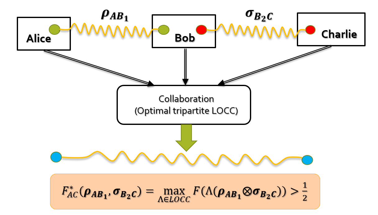
Figure 1: (Color online) Alice-Bob share a two-qubit state $\rho_{AB_{1}}$, whereas Bob-Charlie share a two-qubit state $\sigma_{B_{2}C}$. The task is to optimally distribute the best possible teleportation channel between Alice-Charlie using three-party TP LOCC (collaboration). The fully entangled fraction of the distributed two-qubit state must be monotone under three-party TP LOCC and is strictly greater than $\frac{1}{2}$.

IV Results

IV.1 Allowed set of TP LOCC protocols

Let us assume that $\rho_{AB_{1}}$ and $\sigma_{B_{2}C}$ are shared between $\mathcal{AB}$ and $\mathcal{BC}$. We first ask the question of which set of TP LOCC protocols is not physically realizable while optimizing FEF. Whether a protocol is physically allowed or not can be answered if one could answer what the necessary conditions are for deterministic state transformation from $\rho_{AB_{1}}\otimes\sigma_{B_{2}C}$ to some two-qubit density matrix $\eta_{AC}$. Let $\Lambda$ be a protocol that deterministically prepares some state $\eta_{AC}$ from the initial pair $(\rho_{AB_{1}},\leavevmode\nobreak\ \sigma_{B_{2}C})$. For this case, $\Lambda$ would be a valid TP LOCC if both of the following conditions are satisfied:

$$(i)\quad F^{*}(\eta_{AC})\leq F^{*}(\rho_{AB_{1}})\quad and\quad F^{*}(\eta_{AC})\leq F^{*}(\sigma_{B_{2}C}).$$

$$(ii)\quad C(\eta_{AC})\leq C(\rho_{AB_{1}})\leavevmode\nobreak\ C(\sigma_{B_{2}C}).$$ (16)

In a more general sense, the protocol $\Lambda$ may prepare some ensemble of two-qubit states, say $\mathcal{E}=\{p_{i},\leavevmode\nobreak\ \eta_{AC,i}\}$ from $\rho_{AB_{1}}\otimes\sigma_{B_{2}C}$. For this case also, $\Lambda$ implies a valid TP LOCC if the conditions $(i)$ and $(ii)$ (i.e., Eq.  (16)) are satisfied while averaging over the ensemble $\mathcal{E}$.

The mentioned conditions $(i)$ and $(ii)$ are necessary for deterministic state transformation from $\mathbb{C}^{2}\otimes\mathbb{C}^{4}\otimes\mathbb{C}^{2}$ to $\mathbb{C}^{2}\otimes\mathbb{C}^{2}$. Here note that condition $(ii)$ is a direct consequence of the observation made in Ref. Gour and Sanders (2004). However, satisfying one of the conditions does not necessarily imply the other to be satisfied in general; since for any two-qubit state $\rho$, $F^{*}(\rho)$ and $C(\rho)$ are independent LOCC monotones. Ergo, if $\Lambda$ violates either of the conditions $(i)$ and $(ii)$, it would not be a valid LOCC state transformation.

Structure of optimal protocols:

Now we will discuss the possible structures of the three-party TP LOCC protocols that are optimal for distributing the best teleportation channel. All such protocols explicitly depend on the preshared states. Consider the $\mathcal{A}|\mathcal{BC}$ bipartition and the fact that $\mathcal{BC}$ can perform any global operation. In that case, Bob and Charlie do not have to remain spatially separated and can be considered in a single lab. However, here Alice-Bob are only allowed to perform LOCC. Now from Ref. Verstraete and Verschelde (2003), it is already known that a one-way LOCC is sufficient for optimizing FEF of any two-qubit state. Hence, for the case where Bob-Charlie are in a single lab, a one-way LOCC from Bob to Alice is sufficient for obtaining the best FEF between Alice-Charlie. So for the given initial state $\eta_{AB_{1}B_{2}C}$ let us consider $\mathcal{S}(\Gamma_{B\rightarrow A}|\eta_{AB_{1}B_{2}C})$ as the set of all such protocols which are one-way LOCC from Bob to Alice ($B\rightarrow A$), where Bob-Charlie perform global operation. Similarly, if one considers $\mathcal{C}|\mathcal{AB}$ bipartition, where Alice-Bob can perform any global operation, then one can consider another set of protocols $\mathcal{S}(\tilde{\Gamma}_{B\rightarrow C}|\eta_{AB_{1}B_{2}C})$ which are one-way LOCC from Bob to Charlie ($B\rightarrow C$) only.

So for the given initial state $\eta=\rho_{AB_{1}}\otimes\sigma_{B_{2}C}$, let $\mathcal{S}(\Lambda^{*}|\leavevmode\nobreak\ \eta)$ denote the set of all optimal three-party TP LOCC protocols that can prepare the best teleportation channel between Alice-Charlie. Then of course the following property

$$\mathcal{S}(\Lambda^{*}|\leavevmode\nobreak\ \eta)\subset\mathcal{S}(\Gamma_{B\rightarrow A}|\leavevmode\nobreak\ \eta)\cap\mathcal{S}(\tilde{\Gamma}_{B\rightarrow C}|\leavevmode\nobreak\ \eta)$$ (17)

should satisfy, where $\Lambda^{*}\in TP\leavevmode\nobreak\ LOCC$ is the optimal protocol.

Set of one-way assisted protocols from Bob to Alice-Charlie:

It is difficult to exactly figure out the set $\mathcal{S}(\Lambda^{*}|\eta_{AB_{1}B_{2}C})$ unless the given initial state $\rho_{AB_{1}}\otimes\sigma_{B_{2}C}$ has some specific property in its state-space structure. In this regard, one can think of a restricted TP LOCC protocol that is a one-way TP LOCC protocol from Bob to Alice-Charlie. Here Bob starts the protocol by performing any finite $m-$outcome POVM, $\{\Pi_{i}=B_{i}^{\dagger}B_{i}\}_{i=0}^{m-1}$, where $\{B_{i}\}$ are the set of Kraus operators. After that, Bob’s system is completely discarded, and depending on the measurement outcome $i$, Alice-Charlie have the freedom to perform local post-processing. So the best that Alice-Charlie can do after Bob’s operation is to perform the optimal post-processing (see Eq.  (9)).

Let $\mathcal{S}(\Lambda_{B\rightarrow AC}|\eta)$ denotes the set of all such one-way TP LOCC protocols assisted by Bob i.e., $\Lambda_{B\rightarrow AC}$ for the given initial state $\eta$. Hence, for such a restricted set of protocols from Bob to Alice-Charlie ($B\rightarrow AC$), the best possible average FEF can be computed as

$$F^{*}_{B\rightarrow AC}(\rho,\sigma) =\max_{\Lambda_{B\rightarrow AC}}F(\Lambda_{B\rightarrow AC}(\eta))$$

$$=\max_{\{\Pi_{i}\}}\sum_{i=0}^{m-1}F^{*}(\rho_{AC,\Pi_{i}})$$

$$\leq F^{*}_{AC}(\rho,\sigma),$$ (18)

where $\Lambda_{B\rightarrow AC}\in\mathcal{S}(\Lambda_{B\rightarrow AC}|\eta)$ and the maximization is taken over the set $\mathcal{S}(\Lambda_{B\rightarrow AC}|\eta)$. Here is the remotely prepared state:

$$\rho_{AC,\Pi_{i}} =\dfrac{1}{Q_{i}}Tr_{B_{1}B_{2}}\left[(\mathbb{I}_{AC}\otimes B_{i})\eta_{AB_{1}B_{2}C}(\mathbb{I}_{AC}\otimes B^{\dagger}_{i})\right],$$

where $Q_{i}=Tr\left[(\mathbb{I}_{AC}\otimes\Pi_{i})\eta_{AB_{1}B_{2}C}\right]$ is the probability of preparing $\rho_{AC,\Pi_{i}}$. Note that the inequality in Eq.  (18) arises because every one-way TP LOCC protocol $\Lambda_{B\rightarrow AC}$ is not an optimal protocol in general. However for a given $\eta$, a strict subset of $\mathcal{S}(\Lambda_{B\rightarrow AC}|\eta)$ can be a subset of the set of optimal protocols i.e. $\mathcal{S}(\Lambda^{*}|\eta)$. Only in that case, the inequality in Eq.  (18) is saturated.

IV.2 Upper bounds on the fully entangled fraction

Proposition 1.

In a three-party network scenario, if Alice-Bob ($\mathcal{AB}$) share a two-qubit state $\rho_{AB_{1}}$ and Bob-Charlie ($\mathcal{BC}$) share a two-qubit state $\sigma_{B_{2}C}$, then under collaboration (under all possible tripartite TP LOCC), the optimal fully entangled fraction (FEF) between Alice-Charlie i.e., $F^{*}_{AC}(\rho,\leavevmode\nobreak\ \sigma)$ has the following upper bound,

$$F^{*}_{AC}(\rho,\leavevmode\nobreak\ \sigma)\leq\min\{F_{1}^{*}(\rho,\sigma),\leavevmode\nobreak\ F_{2}^{*}(\rho,\sigma)\},$$ (19)

where $$F_{1}^{*}=\min\{F^{*}(\rho_{AB_{1}}),\leavevmode\nobreak\ F^{*}(\sigma_{B_{2}C})\},$$ (20)

and $$F_{2}^{*}=\dfrac{1}{2}\left(1+C(\rho_{AB_{1}})\leavevmode\nobreak\ C(\sigma_{B_{2}C})\right),$$ (21)

where $C(\rho)$ denotes the concurrence of a two-qubit state $\rho$.

Proof.

In the proof, first we need to show whether $F^{*}_{AC}(\rho,\leavevmode\nobreak\ \sigma)\leq F_{1}^{*}(\rho,\sigma)$ and $F^{*}_{AC}(\rho,\leavevmode\nobreak\ \sigma)\leq F_{2}^{*}(\rho,\sigma)$ hold or not. The former inequality can be trivially argued from the concept of any LOCC monotone. Note that in the $\mathcal{A}\leavevmode\nobreak\ |\leavevmode\nobreak\ \mathcal{BC}$ bipartition, the optimal FEF cannot exceed the value $F^{*}(\rho_{AB_{1}})$, whether or not $\mathcal{BC}$ can perform any global operation. Same argument holds for $\mathcal{C}\leavevmode\nobreak\ |\leavevmode\nobreak\ \mathcal{AB}$ bipartition. So no tripartite TP LOCC operation can prepare a bipartite two-qubit state with optimal FEF exceeding the value, $F_{1}^{*}(\rho,\sigma)=\min\{F^{*}(\rho_{AB_{1}}),\leavevmode\nobreak\ F^{*}(\sigma_{B_{2}C})\}$.

Now we need to show whether $F^{*}_{AC}(\rho,\leavevmode\nobreak\ \sigma)\leq F_{2}^{*}(\rho,\sigma)$ holds or not. The proof directly follows from the observations in Ref. Verstraete and Verschelde (2003) and Ref. Gour and Sanders (2004). As per the definition of the optimal FEF of any two-qubit state, we know that $F^{*}(\rho)$ is always upper bounded as (see Eq.  (7))

$$F^{*}(\rho)\leq\dfrac{1}{2}\left(1+C(\rho)\right).$$ (22)

In Ref. Gour and Sanders (2004) it has been shown that if $\mathcal{AB}$ share a two-qubit state $\rho_{AB_{1}}$ and $\mathcal{BC}$ share $\sigma_{B_{2}C}$ then under all possible tripartite TP LOCC, the average concurrence between Alice-Charlie cannot exceed the bound $C(\rho_{AB_{1}})\leavevmode\nobreak\ C(\sigma_{B_{2}C})$. Now with this observation and by following Eq.  (22) one can easily conclude that optimal average FEF between Alice-Charlie is upper bounded by

$$F^{*}_{AC}(\rho,\leavevmode\nobreak\ \sigma)\leq\dfrac{1}{2}\left(1+C(\rho_{AB_{1}})\leavevmode\nobreak\ C(\sigma_{B_{2}C})\right)=F_{2}^{*}(\rho,\sigma).$$ (23)

The upper bounds $F_{1}^{*}(\rho,\sigma)$ and $F_{2}^{*}(\rho,\sigma)$ are independent:

The upper bounds $F_{1}^{*}(\rho,\sigma)$ and $F_{2}^{*}(\rho,\sigma)$ introduced in Proposition 1 are in general independent of each other. Hence, if one of the bounds is saturated the other one becomes unachievable in general. So in different instances, one can show that both the conditions, $F_{1}^{*}(\rho,\sigma)\geq F_{2}^{*}(\rho,\sigma)$ and $F_{1}^{*}(\rho,\sigma)\leq F_{2}^{*}(\rho,\sigma)$ are possible.

When $F_{1}^{*}(\rho,\sigma)\leq F_{2}^{*}(\rho,\sigma)$ is satisfied:

Let $\mathcal{AB}$ share a two-qubit state $\rho_{AB_{1}}$ and $\mathcal{BC}$ share a Bell state $\ket{\Phi_{0}}_{B_{2}C}$ (see Eq.  (11)). For such a pair of preshared states, one can trivially show that the optimal FEF satisfies,

$$F^{*}_{AC}(\rho,\leavevmode\nobreak\ \sigma) =F_{1}^{*}(\rho,\sigma)=F^{*}(\rho_{AB_{1}}),$$ (24)

The reason is that $\mathcal{BC}$ are sharing a perfect teleportation channel between them, Bob can perfectly teleport one part of $\rho_{AB_{1}}$ to Charlie. As a result, $\mathcal{AC}$ end up with the original preshared state $\rho_{AB_{1}}$. So with all possible tripartite TP LOCC, $\mathcal{AC}$ cannot yield FEF better than $F^{*}(\rho_{AB_{1}})$. Hence, the bound $F_{1}^{*}(\rho,\sigma)$ is saturated here.

For such an instance, the upper bound $F_{2}^{*}(\rho,\sigma)$ can be expressed as

$$F_{2}^{*}(\rho,\sigma)=\dfrac{1+C(\rho_{AB_{1}})\leavevmode\nobreak\ C(\ket{\Phi_{0}}_{B_{2}C})}{2}=\dfrac{1+C(\rho_{AB_{1}})}{2}.$$ (25)

However, if we choose $\rho_{AB_{1}}=p\ket{\Phi_{0}}\bra{\Phi_{0}}+(1-p)\ket{01}\bra{01}$ with $0<p<1$, then one can always show that $F^{*}(\rho_{AB_{1}})<F_{2}^{*}(\rho,\sigma)$. So this example implies that $F_{1}^{*}(\rho,\sigma)<F_{2}^{*}(\rho,\sigma)$.

When $F_{1}^{*}(\rho,\sigma)\geq F_{2}^{*}(\rho,\sigma)$ is satisfied:

Let us consider a scenario, where $\mathcal{AB}$ share a two-qubit pure partially entangled state $\ket{\Psi}_{AB_{1}}$ and $\mathcal{BC}$ share another two-qubit pure partially entangled state $\ket{\Phi}_{B_{2}C}$ such that $C(\ket{\Psi}_{AB_{1}})<C(\ket{\Phi}_{B_{2}C})<1$.

The FEF $F(\Psi)$ of any two-qubit pure entangled state $\ket{\Psi}$ can be expressed as Verstraete and Verschelde (2002)

$$F(\Psi)=F^{*}(\Psi)=\dfrac{1+C(\Psi)}{2},$$ (26)

which is already a LOCC monotone and is proportional to the concurrence. Now considering our three-party case, no TP LOCC protocol can prepare a pure entangled state between Alice-Charlie whose concurrence exceeds the bound $C(\ket{\Psi}_{AB_{1}})C(\ket{\Phi}_{B_{2}C})$ Gour and Sanders (2004). In Ref. Gour and Sanders (2004), it is shown that there exists a TP LOCC protocol which remotely prepares a two-qubit pure state with the best possible concurrence. Hence, the best possible FEF that $\mathcal{AC}$ can expect is

$$F^{*}_{AC}(\rho,\leavevmode\nobreak\ \sigma)=F_{2}^{*}(\rho,\sigma)=\dfrac{1+C(\ket{\Psi}_{AB_{1}})C(\ket{\Phi}_{B_{2}C})}{2}.$$ (27)

On the other hand, one can always argue that $F^{*}_{AC}(\rho,\leavevmode\nobreak\ \sigma)<F_{1}^{*}(\rho,\sigma)=\min\{F^{*}(\ket{\Psi}_{AB_{1}}),F^{*}(\ket{\Phi}_{B_{2}C})\}$. Hence, the upper bound

$$F^{*}_{AC}(\rho,\leavevmode\nobreak\ \sigma)\leq\min\{F_{1}^{*}(\rho,\sigma),F_{2}^{*}(\rho,\sigma)\}.$$ (28)

holds in general. Hence Proposition 1 is proved. ∎

IV.3 Instances where a subset of Bob-assisted TP LOCC protocols are optimal

We have already introduced the set of one-way TP LOCC protocols from Bob to Alice-Charlie denoted as $\mathcal{S}(\Lambda_{B\rightarrow AC}|\eta)$. We now discuss under which specific cases a strict subset of $\mathcal{S}(\Lambda_{B\rightarrow AC}|\eta)$ becomes a subset of the set of optimal TP LOCC protocols $\mathcal{S}(\Lambda^{*}|\leavevmode\nobreak\ \eta)$. In each of these instances, the average FEF $F^{*}_{B\rightarrow AC}(\rho,\sigma)$ defined in Eq.  (18) becomes equal with the optimal FEF of collaboration i.e., $F_{AC}^{*}(\rho,\sigma)$.

Proposition 2.

Let Alice-Bob ($\mathcal{AB}$) share a two-qubit state $\rho_{AB_{1}}$ and Bob-Charlie $(\mathcal{BC})$ share a two-qubit state $\sigma_{B_{2}C}$, then if there exists a one-way TP LOCC protocol $\Lambda_{B\rightarrow AC}$ from Bob to Alice-Charlie which deterministically prepares a two-qubit state $\chi_{AC}$ between Alice-Charlie such that the following condition is satisfied,

$$\chi_{AC}^{\Gamma_{C}}\leavevmode\nobreak\ \ket{\Phi}=-\dfrac{C(\rho_{AB_{1}})C(\sigma_{B_{2}C})}{2}\leavevmode\nobreak\ \ket{\Phi},$$ (29)

$${\text{w}here,}\quad \Lambda_{B\rightarrow AC}(\rho_{AB_{1}}\otimes\sigma_{B_{2}C})=\chi_{AC},$$

and $\Gamma_{C}$ is the partial transposition w.r.t Charlie and $\ket{\Phi}$ is a MES, then such a protocol is optimal i.e., $\Lambda_{B\rightarrow AC}\in\mathcal{S}(\Lambda^{*}|\rho\otimes\sigma)$. For such a case the optimal FEF of $\chi_{AC}$ is the optimal FEF of collaboration, saturating one of the upper bounds i.e., $F^{*}(\chi_{AC})=F_{AC}^{*}(\rho,\sigma)=F_{2}^{*}(\rho,\sigma)$.

Proof.

The proof is very straightforward. For a given preshared state $\eta_{AB_{1}B_{2}C}=\rho_{AB_{1}}\otimes\sigma_{B_{2}C}$, let $\Lambda_{B\rightarrow AC}$ be a one-way TP LOCC protocol from Bob to Alice-Charlie. Hence, such protocol either deterministically prepares a two-qubit state $\chi_{AC}$ or may prepare a collection of two-qubit states $\mathcal{E}=\{q_{i},\leavevmode\nobreak\ \chi_{AC,i}\}$, where $q_{i}$ denotes the probability of obtaining $\chi_{AC,i}$. The optimal FEF of any two-qubit $\rho$ state cannot exceed the bound given in Eq.  (7) and it is saturated iff the condition in Eq.  (8) is satisfied. Therefore, the protocol $\Lambda_{B\rightarrow AC}$ must be chosen in such a way that either of the conditions

$$\chi_{AC}^{\Gamma_{C}}\leavevmode\nobreak\ \ket{\Phi}=-\dfrac{C(\rho_{AB_{1}})C(\sigma_{B_{2}C})}{2}\leavevmode\nobreak\ \ket{\Phi},$$ (30)

$$or,\quad \chi_{AC,i}^{\Gamma_{C}}\leavevmode\nobreak\ \ket{\Phi_{i}}=-\dfrac{C(\chi_{AC,i})}{2}\leavevmode\nobreak\ \ket{\Phi_{i}},\quad\forall i$$

must hold, where the average concurrence becomes $\sum_{i}q_{i}\leavevmode\nobreak\ C(\chi_{AC,i})=C(\rho_{AB_{1}})C(\sigma_{B_{2}C})$ and $\ket{\Phi}$ as well as every $\ket{\Phi_{i}}$ are MES. Hence, the optimal average FEF can be computed as

$$F^{*}(\chi_{AC})=\sum_{i}q_{i}\leavevmode\nobreak\ F^{*}(\chi_{AC,i}) =\dfrac{1+C(\rho_{AB_{1}})C(\sigma_{B_{2}C})}{2}$$

$$=F_{2}^{*}(\rho,\sigma).$$ (31)

Note here that for a given pair of preshared states, if such assisted protocol(s) exists i.e., $\{\Lambda_{B\rightarrow AC}\}$ satisfying Eq.  (29), then such protocol(s) also maximizes the average concurrence. This is due to the fact that under three-party TP LOCC, the average concurrence is always upper bounded by the value $C(\rho_{AB_{1}})C(\sigma_{B_{2}C})$. Next, we see for a specific class of preshared states whether such protocol(s) exists or not. ∎

Corollary 1.

If $\mathcal{AB}$ share any pure entangled state $\ket{\Psi}_{AB_{1}}$ with concurrence $C_{AB_{1}}$ and $\mathcal{BC}$ share any pure entangled state $\ket{\Phi}_{B_{2}C}$ with concurrence $C_{B_{2}C}$, then the optimal FEF $F^{*}_{AC}(\rho,\leavevmode\nobreak\ \sigma)$ between Alice-Charlie can be expressed as

$$F^{*}_{AC}(\rho,\leavevmode\nobreak\ \sigma)=\dfrac{1+C_{AB_{1}}C_{B_{2}C}}{2},$$ (32)

and the optimal TP LOCC protocol is a one-way LOCC from Bob to Alice-Charlie, where Bob first performs a projection-valued measurement (PVM) in maximally entangled states (MES) and depending on the outcome, Alice-Charlie apply local unitary corrections accordingly.

Proof.

The proof is straightforward and the exact expression of the optimal FEF of collaboration i.e., $F^{*}(\Psi,\Phi)$ is already explained in the proof of Proposition 1. Here we discuss the optimal protocol that supports Proposition 2. The optimal protocol is known as the RPBES protocol Gour and Sanders (2004). So without any loss of generality, let us consider the preshared states, $\ket{\Psi}_{AB_{1}}$ and $\ket{\Phi}_{B_{2}C}$ have the Schmidt decomposition as $\ket{\Psi}_{AB_{1}}=\sqrt{\lambda_{0}}\ket{00}+\sqrt{\lambda_{1}}\ket{11}$, where $\lambda_{0}\geq\lambda_{1}>0$, and $\ket{\Phi}_{B_{2}C}=\sqrt{\eta_{0}}\ket{00}+\sqrt{\eta_{1}}\ket{11}$, where $\eta_{0}\geq\eta_{1}>0$. The RPBES protocol dictates that Bob should first perform a PVM in a basis with the following four basis elements:

$$\ket{P_{k,l}}_{B_{1}B_{2}}=\dfrac{1}{2}\sum_{m,m^{\prime}=0}^{1}e^{i\left[\frac{\pi}{2}(2k+l)(2m+m^{\prime})+\pi\leavevmode\nobreak\ mm^{\prime}\right]}\leavevmode\nobreak\ \ket{m\leavevmode\nobreak\ m^{\prime}},$$ (33)

where $k,l\in\{0,1\}$. Afterward, Bob sends the outcome information $kl$ to Charlie by sending 2 cbits and $l$ to Alice by sending 1 cbit. Depending on $kl$ Charlie performs a unitary correction,

$$U_{C}^{(k,l)}\ket{m^{\prime}}=e^{i\frac{\pi}{2}(2k+l)m^{\prime}}\ket{m^{\prime}},$$ (34)

whereas, Alice performs another unitary correction

$$V_{A}^{l}\ket{m}=e^{i\pi lm}\ket{m}.$$ (35)

So finally the remotely prepared state between Alice-Charlie is

$$\ket{\chi}_{AC}=\sum_{m,m^{\prime}=0}^{1}e^{i\pi mm^{\prime}}\sqrt{\lambda_{m}\eta_{m^{\prime}}}\ket{mm^{\prime}},$$ (36)

where note that $\ket{\chi_{AC}}$ satisfies the condition given in Eq.  (29) and the concurrence of $\ket{\chi}_{AC}$ is $C_{AB_{1}}C_{B_{2}C}$ and the FEF value,

$$F(\chi_{AC})=F^{*}_{AC}(\rho,\leavevmode\nobreak\ \sigma)=\dfrac{1+C_{AB_{1}}C_{B_{2}C}}{2}.$$ (37)

∎

Proposition 3.

If $\mathcal{AB}$ share an arbitrary two-qubit state $\rho_{AB_{1}}$ and $\mathcal{BC}$ share a MES and vice versa, otherwise if $\mathcal{AB}$ share a class of two-qubit entangled states $\rho_{AB_{1}}$, with rank two (containing one product basis in its support) and $\mathcal{BC}$ share a two-qubit pure entangled state $\sigma_{B_{2}C}=\ket{\phi}\bra{\phi}$ (not necessarily a MES) such that the inequality $F^{*}(\rho_{AB_{1}})<F^{*}(\sigma_{B_{2}C})$ holds and vice versa, then there exists a set of Bob assisted protocols i.e., $\mathcal{S}(\Lambda_{B\rightarrow AC}|\eta)$ which are optimal. For such a case, the optimal average FEF becomes the optimal FEF of collaboration i.e., $F^{*}_{AC}(\rho,\sigma)$, that saturates the upper bound i.e., $F^{*}_{AC}(\rho,\sigma)=F_{1}^{*}(\rho,\sigma)$.

Proof.

If $\mathcal{AB}$ share an arbitrary two-qubit state $\rho_{AB_{1}}$ and $\mathcal{BC}$ share a Bell state $\ket{\Phi_{0}}$, then Bob can perfectly teleport the qubit system $B_{1}$ to Charlie using standard teleportation protocol Horodecki et al. (1996). After unitary correction by Charlie, exactly $\rho_{AB_{1}}$ is prepared between Alice-Charlie. After this, Alice-Charlie perform optimal local post-processing and can at most achieve optimal FEF not exceeding $F^{*}(\rho_{AB_{1}})$. So in this case, the optimal FEF of collaboration trivially hits the upper bound $F_{1}^{*}(\rho,\sigma)$. The other scenario, though, is not quite so simple.

Let $\mathcal{AB}$ now share a rank two mixed state of the form $\rho_{AB_{1}}=(\Lambda_{ADC}\otimes\mathbb{I})\ket{\psi}_{AB_{1}}\bra{\psi}$, where $\ket{\psi}_{AB_{1}}=\sqrt{\alpha_{0}}\ket{00}+\sqrt{\alpha_{1}}\ket{11}$ such that the Schmidt coefficients are $\alpha_{0}\geq\alpha_{1}>0$. Here $\Lambda_{ADC}$, being the amplitude damping channel (ADC), is a non-unital channel locally acting on Alice’s system. Note that $\Lambda_{ADC}$ has Kraus operators, $K_{0}=|0\rangle\langle 0|+\sqrt{1-p}|1\rangle\langle 1|$ and $K_{1}=\sqrt{p}|0\rangle\langle 1|+|1\rangle\langle 0|$ respectively, where $p\in(0,1)$ is the channel parameter. So the representation of the noisy state $\rho_{AB_{1}}$ can be expressed as

$$\rho_{AB_{1}} =(1-p\alpha_{1})|\chi_{p}\rangle\langle\chi_{p}|+p\alpha_{1}|01\rangle\langle 01|,$$ (38)

$$\text{where,}\leavevmode\nobreak\ \ket{\chi_{p}} =\frac{1}{\sqrt{1-p\alpha_{1}}}\left(\sqrt{\alpha_{0}}\ket{00}+\sqrt{1-p}\sqrt{\alpha_{1}}\ket{11}\right)$$ (39)

From Eq.  (38), one can compute the optimal FEF of the preshared state $\rho_{AB_{1}}$ as

$$F^{*}(\rho_{AB_{1}}) =\dfrac{1}{2}(1+C(\rho_{AB_{1}})-p\alpha_{1}),\leavevmode\nobreak\ \leavevmode\nobreak\ \textit{if}\leavevmode\nobreak\ \leavevmode\nobreak\ C(\rho_{AB_{1}})\geq 2p\alpha_{1},$$

$$=\dfrac{1}{2}\left(1+\alpha_{0}\dfrac{1-p}{p}\right),\quad\textit{if}\leavevmode\nobreak\ \leavevmode\nobreak\ C(\rho_{AB_{1}})<2p\alpha_{1},$$ (40)

where $C(\rho_{AB_{1}})=2\sqrt{\alpha_{0}\leavevmode\nobreak\ \alpha_{1}}\sqrt{1-p}$ is the concurrence of $\rho_{AB_{1}}$. Furthermore from Eq.  (40) one can easily conclude that

$$F^{*}(\rho_{AB_{1}})<\dfrac{1+C(\rho_{AB_{1}})}{2}.$$

We now assume a scenario, where $\mathcal{BC}$ share a pure two-qubit entangled state, say, $\ket{\phi}_{B_{2}C}=\sqrt{\beta_{0}}\ket{00}+\sqrt{\beta_{1}}\ket{11}$ such that $\beta_{0}\geq\beta_{1}>0$. Moreover, we assume that

$$F^{*}(\rho_{AB_{1}})<F^{*}(\ket{\phi}_{B_{2}C})=\dfrac{1+C(\phi)}{2}$$

is satisfied which signifies $\mathcal{AB}$ initially share a worst teleportation channel. Now we will show that under some specific range of state parameters of $\rho_{AB_{1}}$ and $\ket{\phi}_{B_{2}C}$, there exists a set of TP LOCC protocols for which one obtains the best possible FEF $F^{*}_{AC}(\rho,\leavevmode\nobreak\ \sigma)$ as

$$F^{*}_{AC}(\rho,\leavevmode\nobreak\ \sigma)=\min\{F_{1}^{*}(\rho,\sigma),\leavevmode\nobreak\ F_{2}^{*}(\rho,\sigma)\}=F_{1}^{*}(\rho,\sigma),$$

$$s.t.,\leavevmode\nobreak\ \leavevmode\nobreak\ F_{1}^{*}(\rho,\sigma)=F^{*}(\rho_{AB_{1}}).$$

Conditions on the state parameters:

The independent state parameters of $\rho_{AB_{1}}$ are $p\in(0,1)$ and $\alpha_{0}\in[\frac{1}{2},1)$, whereas for $\ket{\phi}_{B_{2}C}$ it is just $\beta_{0}\in[\frac{1}{2},1)$. We are interested in the domain where

$$\frac{1}{2}\leq\alpha_{0}<\frac{p^{2}}{1-p+p^{2}},\quad\text{while}\leavevmode\nobreak\ \leavevmode\nobreak\ \frac{\sqrt{5}-1}{2}<p<1.$$

and, $$\frac{1}{2}\leq\beta_{0}<\frac{\alpha_{1}\leavevmode\nobreak\ p^{2}}{p^{2}+\alpha_{0}(1-p-p^{2})}.$$ (41)

are satisfied.

Optimal protocol:

It can be shown if the parameters $(p,\leavevmode\nobreak\ \alpha_{0},\leavevmode\nobreak\ \beta_{0})$ lie in the above domain, there exists a set of optimal TP LOCC protocols which are one-way LOCC protocols from Bob to Alice and Charlie. However, these protocols are sufficient and may not be the only protocols. In each of the protocols, Bob first performs a PVM measurement in the following equally entangled basis,

$$\ket{\eta_{0}}=\sqrt{\delta_{0}}\ket{00}+\sqrt{\delta_{1}}\ket{11},\leavevmode\nobreak\ \ket{\eta_{1}}=\sqrt{\delta_{1}}\ket{00}-\sqrt{\delta_{0}}\ket{11}$$

$$\ket{\eta_{2}}=\sqrt{\delta_{0}}\ket{01}+\sqrt{\delta_{1}}\ket{10},\leavevmode\nobreak\ \ket{\eta_{3}}=\sqrt{\delta_{1}}\ket{01}-\sqrt{\delta_{0}}\ket{10}$$ (42)

where $\delta_{0}\geq\delta_{1}>0$ and further restriction on the PVM basis is

$$\dfrac{1}{2}\leq\delta_{0}<\dfrac{p^{2}(1-\alpha_{0}-\beta_{0}+\alpha_{0}\beta_{0})}{\alpha_{0}\beta_{0}(1-p)+p^{2}(1-\alpha_{0}-\beta_{0}+\alpha_{0}\beta_{0})}.$$ (43)

So note here that for a given choice of preshared states $\rho_{AB_{1}}$ and $\ket{\phi}_{B_{2}C}$ with parameters chosen from the domain (given in Eq.  (41)), there exists a set of PVM measurements (in Eq.  (42)) that can be performed by Bob. After this, Bob’s system is discarded and Alice-Charlie end up with a post-measurement state (see Appendix A for details)

$$\rho_{AC,\eta_{i}}=(\Lambda_{ADC}\otimes\mathbb{I})|\xi_{i}\rangle\langle\xi_{i}|,$$

where $\ket{\xi_{i}}=\sqrt{\gamma_{0,i}}\ket{00}+\sqrt{\gamma_{1,i}}\ket{11}$ such that $\gamma_{0,i}$ is the largest Schmidt coefficient and is a function of the parameters $p,\leavevmode\nobreak\ \alpha_{0},\leavevmode\nobreak\ \beta_{0},\leavevmode\nobreak\ \delta_{0}$. Note here that the probability of obtaining $\rho_{AC,\eta_{i}}$ is $P_{i}=\frac{1}{4}$.

After preparing $\rho_{AC,\eta_{i}}$, Charlie next performs a two-outcome POVM operation $\{A_{0,i}^{\dagger}A_{0,i},\leavevmode\nobreak\ \mathbb{I}-A_{0,i}^{\dagger}A_{0,i}\}$ depending on the outcome $i$. Here the POVM element $A_{0,i}^{\dagger}A_{0,i}$ has the form

$$A_{0,i}^{\dagger}A_{0,i}=\left(\begin{array}[]{cc}1&0\\ 0&\dfrac{\gamma_{0,i}}{\gamma_{1,i}}\dfrac{1-p}{p^{2}}\end{array}\right),$$ (46)

$$s.t.,\leavevmode\nobreak\ \leavevmode\nobreak\ \sqrt{\gamma_{0,i}\leavevmode\nobreak\ (1-p)}<p\sqrt{\gamma_{1,i}}$$ (47)

holds. So if the first outcome appears, Alice does nothing, otherwise, they replace the state with a product state. So after averaging over all outcome the average FEF of Alice-Charlie can be expressed as

$$\frac{1}{4}\sum_{i=0}^{3}F^{*}(\rho_{AC,\eta_{i}})=F_{1}^{*}(\rho,\sigma)=F^{*}(\rho_{AB_{1}}).$$

Therefore, one can easily argue that the best possible FEF under collaboration is $F^{*}_{AC}(\rho,\leavevmode\nobreak\ \sigma)=\frac{1}{4}\sum_{i}F^{*}(\rho_{AC,\eta_{i}})$. ∎

Remark:

There is an interesting observation in Proposition 3. Suppose $\mathcal{AB}$ initially share an entangled state $\rho_{AB_{1}}$ that is an imperfect resource for teleportation. Now with this already existing noisy state $\rho_{AB_{1}}$, intuition suggests that distributing a two-qubit state between Alice-Charlie with the best possible teleportation fidelity, Bob needs to perfectly teleport one of his qubits which is entangled with Alice, and for this $\mathcal{BC}$ must share a MES. With this, exactly $\rho_{AB_{1}}$ will be distributed between Alice and Charlie, and then Alice-Charlie can perform optimal post-processing to obtain the best possible FEF $F^{*}_{AC}(\rho,\leavevmode\nobreak\ \sigma)$. However, this is not the only way to obtain $F^{*}_{AC}(\rho,\leavevmode\nobreak\ \sigma)$. Even if $\mathcal{BC}$ share a non-maximal pure entangled state (an imperfect teleportation channel) then also there exists a protocol via which Alice-Charlie can achieve FEF same as $F^{*}_{AC}(\rho,\leavevmode\nobreak\ \sigma)$. Moreover, in each of the TP LOCC protocols, joint two-qubit measurement by Bob in a complete MES basis is sufficient but not necessary. This observation infers that the optimal distribution of a general teleportation channel does not necessarily imply perfectly teleporting a part of an entangled state to the receiver.

Proposition 4.

If $\mathcal{AB}$ share an entangled Bell-diagonal state $\rho_{AB_{1}}=\sum_{i=0}^{3}p_{i}\ket{\Phi_{i}}\bra{\Phi_{i}}$ and $\mathcal{BC}$ share another entangled Bell-diagonal state $\sigma_{B_{2}C}=\sum_{j=0}^{3}q_{j}\ket{\Phi_{j}}\bra{\Phi_{j}}$, then with collaboration, the best possible FEF between Alice-Charlie can be expressed as

$$F^{*}_{AC}(\rho,\leavevmode\nobreak\ \sigma) =\lambda_{max}\left[(\Lambda_{p}\circ\tilde{\Lambda}_{q}\otimes\mathbb{I})\leavevmode\nobreak\ P_{\Phi_{0}}\right]$$

$$\leq min\{F_{1}^{*}(\rho,\sigma),F_{2}^{*}(\rho,\sigma)\},$$ (48)

where $P_{\Phi_{0}}=\ket{\Phi_{0}}\bra{\Phi_{0}}$, and $\{\ket{\Phi_{i}}\}$ forms complete orthonormal Bell basis $($Eq.  (11)$)$. $\lambda_{max}(\rho)$ is the largest eigenvalue of any density matrix $\rho$ and $\{\Lambda_{p},\tilde{\Lambda}_{q}\}$ are unital qubit channels with Kraus operators $\{\sqrt{p_{i}}\leavevmode\nobreak\ \sigma_{i}\}$ and $\{\sqrt{q_{j}}\leavevmode\nobreak\ \sigma_{j}^{*}\}$ respectively, $\sigma_{i}$s being the Pauli matrices.

The detailed proof of this proposition is given in Appendix B and in the proof of Proposition 5. One important point to note here is that the optimal FEF of collaboration $F^{*}_{AC}(\rho,\sigma)$ in Eq.  (48) must strictly larger than $\frac{1}{2}$. Equivalently, the concatenated unital channel $\Lambda_{p}\circ\tilde{\Lambda}_{q}$ must not be entanglement breaking, otherwise we have $F^{*}_{AC}(\rho,\sigma)=\frac{1}{2}$. This implies that not all the preshared entangled Bell diagonal states are useful here, rather a subset of them must be chosen such that we have $F^{*}_{AC}(\rho,\leavevmode\nobreak\ \sigma)>\frac{1}{2}$.

Proposition 5.

The collaborative optimal TP LOCC protocol for achieving the optimal FEF in Eq.  (48) is a one-way LOCC from Bob to Alice-Charlie, where Bob performs PVM in MES and Alice-Charlie perform local unitary corrections accordingly.

Proof.

Let us assume that $\mathcal{AB}$ share an entangled state of Bell mixtures $\rho_{AB_{1}}=\sum_{i=0}^{3}p_{i}\ket{\Phi_{i}}\bra{\Phi_{i}}$, and $\mathcal{BC}$ share $\sigma_{B_{2}C}=\sum_{j=0}^{3}q_{j}\ket{\Phi_{j}}\bra{\Phi_{j}}$ which is also entangled. Here, $\{\ket{\Phi_{i}}\}$ forms complete orthonormal Bell basis (see Eq.  (11)) and without any loss of generality one can assume that $p_{0}\geq p_{1}\geq p_{2}\geq p_{3}\geq 0$ and $q_{0}\geq q_{1}\geq q_{2}\geq q_{3}\geq 0$. The only condition via which one can say that both $\rho_{AB_{1}}$ and $\sigma_{B_{2}C}$ are entangled is when the largest eigenvalues $p_{0}$ and $q_{0}$ are strictly larger than $\frac{1}{2}$.

Now to obtain the structure of the optimal protocol, one needs to know the properties of the preshared states. For instance, the FEF of both the preshared states has the form,

$$F(\rho_{AB_{1}})=F^{*}(\rho_{AB_{1}})=\dfrac{1+C(\rho_{AB_{1}})}{2},$$

$$F(\sigma_{B_{2}C})=F^{*}(\sigma_{B_{2}C})=\dfrac{1+C(\sigma_{B_{2}C})}{2},$$

which are of course LOCC monotones. So if Alice or Charlie starts the protocol, they can only perform local unitary operations, otherwise, the protocol will not be optimal. This is because even if Bob-Charlie come to a common lab, then in $\mathcal{A}|\mathcal{BC}$ bipartition, the FEF of the preshared state cannot increase beyond $F^{*}(\rho_{AB_{1}})$. So Alice has no option to perform any operation except local unitary. The same argument follows for Charlie also, while considering $\mathcal{C}|\mathcal{AB}$ bipartition. So without any loss of generality, Bob can start the protocol.

Bob performs PVM:

Suppose Bob performs PVM in any entangling basis, say $\{\ket{\psi_{i}^{*}}\}$. Then after the $k^{th}$ outcome, Alice and Charlie end up with the state (for detailed analysis see Appendix B)

$$\rho_{AC}(\psi_{k})=(\Lambda_{p}\otimes\Lambda_{q})\ket{\psi_{k}}_{AC}\bra{\psi_{k}},$$ (49)

with probability $P_{k}=\frac{1}{4}$. Here $\Lambda_{p}$ and $\Lambda_{q}$ are two general Pauli channels with Kraus operators $\{\sqrt{p_{i}}\sigma_{i}\}$ and $\{\sqrt{q_{j}}\sigma_{j}\}$ respectively. Note that $\{p_{i}\}$ and $\{q_{j}\}$ are the eigenvalues of the preshared states. So the optimal FEF between Alice-Charlie for this PVM-assisted protocol can be expressed as

$$F^{*}_{AC,PVM}=\dfrac{1}{4}\max_{PVM}\sum_{k=0}^{3}\leavevmode\nobreak\ F^{*}(\rho_{AC}^{(k)}),$$ (50)

where $F^{*}(\rho_{AC}^{(k)})$ denotes the optimal FEF of $\rho_{AC}(\psi_{k})$ after optimal post-processing by Alice-Charlie. Note here that performing PVM in a complete basis $\{\ket{\psi^{\prime}_{0}},\ket{\psi^{\prime}_{1}},\ket{\psi^{\prime}_{2}},\ket{\psi^{\prime}_{3}}\}$, Bob can prepare four possible states between Alice-Charlie as $\{\rho_{AC}(\psi^{\prime}_{0}),\rho_{AC}(\psi^{\prime}_{1}),\rho_{AC}(\psi^{\prime}_{2}),\rho_{AC}(\psi^{\prime}_{3})\}$. If the choice of basis $\{\ket{\psi^{\prime}_{0}},\ket{\psi^{\prime}_{1}},\ket{\psi^{\prime}_{2}},\ket{\psi^{\prime}_{3}}\}$ is optimal then one can argue that

$$F(\rho_{AC,\psi^{\prime}_{i}}) =\max_{\ket{\Phi}\in MES}\max_{\ket{\psi_{i}}}\bra{\Phi}\rho_{AC}(\psi_{i})\ket{\Phi}$$

$$=\max_{\ket{\Phi}}\max_{\Gamma\in LOCC}\max_{\ket{\psi_{i}}}\bra{\Phi}\Gamma(\rho_{AC}(\psi_{i}))\ket{\Phi}$$

$$=F^{*}(\rho_{AC,\psi^{\prime}_{i}}).$$ (51)

In Ref. Pal et al. (2014) it has been shown that if Alice sends one part of a two-qubit pure entangled state $\ket{\psi}$ to Bob through any qubit channel $\Lambda$, then the best possible FEF attainable through the channel is

$$F(\Lambda) =\max_{\ket{\Phi}}\max_{\Gamma\in LOCC}\max_{\ket{\psi}}\bra{\Phi}\Gamma(\rho_{\Lambda,\psi})\ket{\Phi}$$

$$=\lambda_{max}(\rho_{\Lambda,\Phi_{0}}),$$ (52)

where $\rho_{\Lambda,\psi}=(\mathbb{I}\otimes\Lambda)\ket{\psi}\bra{\psi}$. The maximization over $\ket{\psi}$ implies optimal pre-processing and once the best input state is shared through $\Lambda$, they can perform the optimal post-processing $\Gamma$. It is shown in Ref. Pal et al. (2014) that if $\Lambda$ is an unital channel then the optimal pre-processed state $\ket{\psi}$ must be a MES. In that case, the shared two-qubit state $\rho_{\Lambda_{u},\psi}$ is a Bell diagonal state up to local unitary correction.

Hence, the choice of PVM basis i.e., $\{\ket{\psi^{\prime}_{0}},\ket{\psi^{\prime}_{1}},\ket{\psi^{\prime}_{2}},\ket{\psi^{\prime}_{3}}\}$ must be any four orthogonal MES, since both $\Lambda_{p}$ and $\Lambda_{q}$ are unital. Using straightforward calculations, one can show that the best possible FEF between Alice-Charlie under PVM-assisted protocol (Bob starts with PVM) becomes (detailed derivation is given in Appendix B)

$$F^{*}_{AC,PVM} =\lambda_{max}\left[(\Lambda_{p}\circ\tilde{\Lambda}_{q}\otimes\mathbb{I})\rho_{\Phi_{0}}\right]$$ (53)

$$\leq\min\{F_{1}^{*}(\rho,\sigma),F_{2}^{*}(\rho,\sigma)\}.$$

Bob performs POVM:

Instead of performing PVM, Bob could perform POVM. Any $N$ outcome POVM elements can be expressed as the collection $\{\pi_{i}\}$ such that $\sum_{i=1}^{N}\pi_{i}=\mathbb{I}$. Without any loss of generality, one can represent each POVM element as

$$\pi_{i}=\sum_{k=0}^{3}q_{i,k}\ket{\psi^{*}_{i,k}}\bra{\psi^{*}_{i,k}},\quad\quad q_{i,k}\geq 0$$

where $\sum_{k}q_{i,k}\leq 1$ and $\{\ket{\psi^{*}_{i,k}}\}$ forms a complete orthonormal basis set. With this approach, it can be easily shown that (for details see Appendix B)

$$F^{*}_{AC,POVM}\leq F^{*}_{AC,PVM}=F^{*}_{AC}(\rho,\leavevmode\nobreak\ \sigma).$$ (54)

Hence, the sufficient protocol that optimally distributes the teleportation channel comprises Bob performing PVM in the standard Bell basis (see Eq.  (11)), whereas Alice and Charlie perform unitary correction (Pauli correction) accordingly. ∎

IV.4 Every Bob-assisted protocol that starts with joint PVM in any MES basis may not be efficient

Proposition 6.

Suppose $\mathcal{AB}$ share a rank two entangled state of the form, $\rho_{AB_{1}}=q|\psi\rangle\langle\psi|+(1-q)|01\rangle\langle 01|$, where $\ket{\psi}=\sqrt{\alpha_{0}}\ket{00}+\sqrt{\alpha_{1}}\ket{11}$ with $0<q<1$ and $\alpha_{0}\geq\alpha_{1}>0$. Whereas, $\mathcal{BC}$ share a weakly entangled Werner state i.e., $\sigma_{B_{2}C}=\lambda|\Phi_{0}\rangle\langle\Phi_{0}|+(1-\lambda)\frac{\mathbb{I}_{4}}{4}$. Then depending on the parameter $\lambda$, there can exist a range $0<q<q_{c}(\lambda)$ for which any Bob-assisted TP LOCC protocol is suboptimal or efficient iff Bob’s operation excludes PVM in any maximally entangled basis.

Proof.

As mentioned previously in Proposition 3 that the structure of $\rho_{AB_{1}}$ has the form

$$\rho_{AB_{1}}=\left(1-\frac{p}{2}\right)|\psi_{p}\rangle\langle\psi_{p}|+\frac{p}{2}|01\rangle\langle 01|,$$

where, $$\ket{\psi_{p}}=\frac{1}{\sqrt{2-p}}\left(\ket{00}+\sqrt{1-p}\ket{11}\right),$$ (55)

and $p\in(0,1)$ is the channel parameter. Notice that $\rho_{AB_{1}}$ has a single channel parameter $p$. We now choose $\sigma_{B_{2}C}$ to be isotropic that means $\sigma_{B_{2}C}$ is a two-qubit Werner state i.e., $\sigma_{B_{2}C}=\lambda|\Phi_{0}\rangle\langle\Phi_{0}|+(1-\lambda)\frac{\mathbb{I}}{4}$ which is entangled if $\lambda>\frac{1}{3}$. Now as per the proposition demands, let us choose $\sigma_{B_{2}C}$ to be weakly entangled. This means that we must choose $\lambda$ to be close to $\frac{1}{3}$. So for instance, let us choose $\lambda=\frac{2}{5}$ such that $\sigma_{B_{2}C}$ is weakly entangled. One can easily estimate that concurrence of $\sigma_{B_{2}C}$ is $0.1$ while $\lambda=\frac{2}{5}$.

Efficient distribution protocol:

For the given choice of preshared states, finding the optimal protocol that distributes the best teleportation channel between Alice and Charlie is hard. However, by considering the property of the preshared states (also see Eq,  (40)), one can estimate

$$F^{*}(\rho_{AB_{1}}) =\frac{1}{2}\left(1+C(\rho_{AB_{1}})-\frac{p}{2}\right),\leavevmode\nobreak\ \leavevmode\nobreak\ \text{if}\leavevmode\nobreak\ \leavevmode\nobreak\ 0<p<\frac{\sqrt{5}-1}{2},$$

$$=\frac{1}{2}\left(1+\frac{1-p}{2p}\right),\leavevmode\nobreak\ \leavevmode\nobreak\ \text{if}\leavevmode\nobreak\ \leavevmode\nobreak\ p>\frac{\sqrt{5}-1}{2},$$

and, $$F^{*}(\sigma_{B_{2}C})=\frac{1+C(\sigma_{B_{2}C})}{2}=\frac{1+3\lambda}{4}.$$ (56)

So if $\mathcal{AB}$ are allowed to do global operation (if they come to a single lab) then considering $\mathcal{C}|\mathcal{AB}$ bipartition, Charlie cannot perform any operation rather than local unitary, since the FEF of $\mathcal{BC}$ is already a LOCC monotone. Therefore there are two different ways to collaborate. Either Alice or Bob can begin the protocol. However, we are only interested in the branch, where Bob starts the protocol. Next, we will show that if Bob starts protocol by performing PVM in any maximally entangled basis, then such protocol is not efficient and of course not optimal.

Bob performs PVM in MES:

Let Bob performs PVM in an arbitrary MES basis, say for example $\{\ket{\Psi_{i}^{*}}\}$, where each of the vector $\ket{\Psi_{i}^{*}}$ can be expressed as (see Appendix C for details)

$$\ket{\Psi^{*}_{i}}=(\mathbb{I}\otimes W^{*}_{i})\ket{\Phi_{0}},\quad i=0,1,2,3,$$ (57)

where $\langle\Psi_{i}|\Psi_{j}\rangle=\delta_{ij}$ and $W_{i}^{*}$ is a unitary from $SU(2)$ for every $i$. The orthogonality condition demands that $Tr(W^{T}_{i}W^{*}_{j})=2\delta_{ij}$. After performing PVM in $\{\ket{\Psi^{*}_{i}}\}$, Alice-Charlie end up with a post-measurement state (see Appendix C for details)

$$\rho_{AC,\Psi_{i}} =(\Lambda_{ADC}\otimes\Lambda_{dep})|\Psi_{i}\rangle\langle\Psi_{i}|$$

$$=(\mathbb{I}\otimes W_{i})(\Lambda_{ADC}\otimes\Lambda_{dep})|\Phi_{0}\rangle\langle\Phi_{0}|(\mathbb{I}\otimes W_{i}^{\dagger}),$$ (58)

which is prepared with probability $P_{i}=\frac{1}{4}$. In Eq.  (58) $\Lambda_{dep}$ represents depolarzing channel with Kraus operators $\{\sqrt{\frac{1+3\lambda}{4}}\mathbb{I},\leavevmode\nobreak\ \sqrt{\frac{1-\lambda}{4}}\sigma_{1},\leavevmode\nobreak\ \sqrt{\frac{1-\lambda}{4}}\sigma_{2},\sqrt{\frac{1-\lambda}{4}}\sigma_{3}\}$. Eq.  (58) also implies that $\rho_{AC,\Psi_{i}}$ is connected with an unique state $\rho_{\Lambda_{ADC},\Lambda_{dep},\Phi_{0}}=(\Lambda_{ADC}\otimes\Lambda_{dep})|\Phi_{0}\rangle\langle\Phi_{0}|$ via local unitary $W_{i}$. So after performing PVM in any MES, Charlie can transform the state to a unique form via unitary correction.

After preparing the $\rho_{AC,\Psi_{i}}$ for every $i$, the best thing Alice-Charlie can do is to perform optimal post-processing (see Eq.  (9)), and with this the average fidelity between Alice-Charlie can be expressed as

$$F^{*}_{AC,\{\Psi_{i}\}} =\sum_{i}P_{i}F^{*}(\rho_{AC,\Psi_{i}})$$

$$=F^{*}(\rho_{\Lambda_{ADC},\Lambda_{dep},\Phi_{0}})\leq F^{*}_{AC}(\rho,\leavevmode\nobreak\ \sigma).$$ (59)

It can be analytically shown that if we fix $\lambda=\frac{2}{5}$, then within a range $\frac{1}{3}<p<1$, every two-qubit state $\rho_{AC,\Psi_{i}}$ is separable, hence,

$$F^{*}_{AC,\{\Psi_{i}\}}=\frac{1}{2}\quad and\quad C(\rho_{AC,\Psi_{i}})=0$$ (60)

if we choose $\lambda=\frac{2}{5}$ and $\frac{1}{3}<p<1$.

Bob performs PVM in partially entangled states:

Now let us consider that Bob performs PVM in some partially entangled states. Of course, the average entanglement cost of such measurement is strictly less than performing PVM in MES. Let us choose the measurement basis as

$$\ket{\eta_{0}}=\frac{\sqrt{3}}{2}\ket{00}+\frac{1}{2}\ket{11},\quad\ket{\eta_{1}}=\frac{1}{2}\ket{00}-\frac{\sqrt{3}}{2}\ket{11},$$

$$\ket{\eta_{2}}=\frac{\sqrt{3}}{2}\ket{01}+\frac{1}{2}\ket{10},\quad\ket{\eta_{3}}=\frac{1}{2}\ket{01}-\frac{\sqrt{3}}{2}\ket{10}.$$

After performing PVM in the above basis, the prepared state between Alice-Charlie can be written as

$$\rho_{AC,\eta_{i}}=(\Lambda_{ADC}\otimes\Lambda_{dep})|\eta_{i}\rangle\langle\eta_{i}|,\quad\quad i=0,1,2,3,$$

which occurs with equal probability $\frac{1}{4}$. Thus, after the state preparation, Alice-Charlie can now perform optimal post-processing on every $\rho_{AC,\eta_{i}}$. Hence, on average the assisted FEF i.e., $F^{*}_{AC,\{\eta_{i}\}}$ can be expressed as (see Appendix C for details)

$$F^{*}_{AC,\{\eta_{i}\}}=\frac{1}{4}\sum_{i=0}^{3}F^{*}(\rho_{AC,\eta_{i}}).$$ (61)

Now if one compares between two aforementioned PVM-assisted TP LOCC protocols then it can be shown that

$$F^{*}_{AC,\{\Psi_{i}\}}<F^{*}_{AC,\{\eta_{i}\}},\quad\text{and,}\quad\overline{C}_{AC,\{\Psi_{i}\}}<\overline{C}_{AC,\{\eta_{i}\}},$$ (62)

while the two conditions, $\lambda=\frac{2}{5}$ and $\frac{1}{3}<p<1$ are satisfied. Here $\overline{C}_{AC,\{\Psi_{i}\}}$ and $\overline{C}_{AC,\{\eta_{i}\}}$ represent the average concurrence for different PVM assisted protocols. So this proclaims that any TP LOCC protocol that starts with Bob’s PVM operation in any MES is not necessarily optimal or even efficient. The comparison is clearly illustrated in Fig. 2 and 3.

Bob performs POVM:

Now suppose that instead of performing PVM, Bob performs a specific five outcome two-qubit POVM whose elements $\{\Pi_{i,B_{1}B_{2}}\}$ are given by (see Appendix C for details)

$$\Pi_{i,B_{1}B_{2}} =B_{i}^{\dagger}B_{i},\quad\quad\quad\quad i=0,1,2,3$$

$$=\left(\sqrt{A_{0}^{\dagger}A_{0}}\otimes\mathbb{I}\right)P_{\Phi_{i}}\left(\sqrt{A_{0}^{\dagger}A_{0}}\otimes\mathbb{I}\right),$$

$$\Pi_{4,B_{1}B_{2}} =\mathbb{I}_{4}-\sum_{i=0}^{3}\Pi_{i,B_{1}B_{2}}=(\mathbb{I}-A_{0}^{\dagger}A_{0})\otimes\mathbb{I},$$ (63)

where $B_{i}=P_{\Phi_{i}}\left(\sqrt{A_{0}^{\dagger}A_{0}}\otimes\mathbb{I}\right)$ is the $i^{th}$ Kraus operator and $P_{\Phi_{i}}=|\Phi_{i}\rangle\langle\Phi_{i}|$ is the projector on the $i^{th}$ Bell basis and $A_{1}^{\dagger}A_{1}=\mathbb{I}_{2}-A_{0}^{\dagger}A_{0}$. Here the operator $A_{0}$ is defined as

$$A_{0}^{\dagger}A_{0}=\left(\begin{array}[]{cc}1&0\\ 0&\frac{1-p}{p^{2}}\end{array}\right).$$ (66)

Note that the operator $A_{0}^{\dagger}A_{0}$ is positive and trace non-increasing iff the channel parameter $p$ lies in the domain $\frac{\sqrt{5}-1}{2}<p<1$. Thus the POVM elements in Eq.  (63) are physical only in a particular range of channel parameter $p$. Now let us fix a specific TP LOCC protocol, where Bob first performs the POVM $\Pi_{i,B_{1}B_{2}}$ and then depending on the outcome $i$, Alice-Charlie again have to perform optimal post-processing on the prepared state. So for $i^{th}$ outcome, if $\rho_{AC,\Pi_{i}}$ is the prepared state between Alice-Charlie then it can be shown that the following strict inequalities appear within $\frac{\sqrt{5}-1}{2}<p<1$ as

$$F^{*}_{AC,\{\Pi_{i}\}}=\sum_{i=0}^{3}Q_{i}\leavevmode\nobreak\ F^{*}(\rho_{AC,\Pi_{i}})>F^{*}(\rho_{\Lambda_{ADC},\Lambda_{dep},\Phi_{0}}),$$

$$\overline{C}_{AC,\{\Pi_{i}\}}>\overline{C}_{AC,\{\Psi_{i}\}}=0,\quad\quad\forall\ket{\Psi_{i}}\in MES$$ (67)

which implies that measurement in POVM that are typically less costly shows a quantum advantage (in terms of distribution of teleportation channel as well as entanglement) over the performance of PVM in any MES basis. Comparison with PVM-assisted protocols is pictorially demonstrated in Fig. 4 and 5.

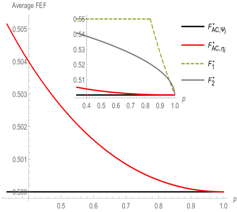
Figure 2: (Color online) The small subfigure is the plots of different PVM-assisted average FEF w.r.t. the channel parameter $p$ of ADC in the range $\frac{1}{3}<p<1$ while $\lambda=\frac{2}{5}$. $F_{1}^{*}(\rho,\sigma)$ and $F_{2}^{*}(\rho,\sigma)$ curves are the plots of two independent LOCC upper bounds (Eq.  (20) and (21)). The larger figure is the magnified version of the smaller one without the plots of $F_{1}^{*}(\rho,\sigma)$ and $F_{2}^{*}(\rho,\sigma)$. The red curve (Eq.  (61)) represents $F^{*}_{AC,\{\eta_{i}\}}$, where Bob performs PVM in non-maximally entangled states (NMES), whereas, the dark horizontal plot (Eq.  (60)) represents all MES assisted FEF, $F^{*}_{AC,\{\Psi_{i}\}}$ which is always $\frac{1}{2}$. This shows clear advantage of PVM-assisted protocol in NMES over PVM-assisted protocols in any MES.

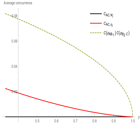
Figure 3: (Color online) Plots of average concurrence for different PVM-assisted protocols w.r.t. the channel parameter $p$ of ADC while $\frac{1}{3}<p<1$ and $\lambda=\frac{2}{5}$. The dashed curve represents the LOCC upper bound on the average concurrence value which is the product of the concurrence of the preshared states. The red curve represents the average concurrence when Bob performs PVM in NMES basis $\{\ket{\eta_{i}}\}$, whereas, the black horizontal line (Eq.  (60)) represents the average concurrence that is zero while Bob performs PVM in any MES basis $\{\ket{\Psi_{i}}\}$.

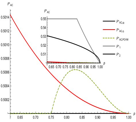
Figure 4: (Color online) The small subfigure contains plots of the average FEF w.r.t. the channel parameter $p$ of ADC for three different assisted protocols (both PVM and POVM) from Bob to Alice-Charlie. It also contains plots of the LOCC upper bounds $F_{1}^{*}(\rho,\sigma)$ and $F_{2}^{*}(\rho,\sigma)$. The larger figure is a magnified version of the smaller one where the plots of $F_{1}^{*}(\rho,\sigma)$ and $F_{2}^{*}(\rho,\sigma)$ are omitted. Here the red curve is for the PVM-assisted protocol in the NMES basis. The dashed curve (see Eq.  (67)) is for POVM-assisted protocol and the black horizontal line is for PVM in any MES. The plots clearly show that within the region $\frac{\sqrt{5}-1}{2}<p<1$, the average FEF from POVM-assisted protocol, i.e., $F^{*}_{AC,\{\Pi_{i}\}}$ can be strictly larger than PVM-assisted protocol in any MES basis.

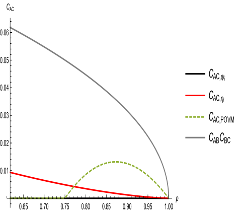
Figure 5: (Color online) Plots of average concurrence w.r.t. the channel parameter $p$ of ADC for different assisted strategies (both PVM and POVM) from Bob to Alice-Charlie. Here the gray curve denotes the upper bound on the average concurrence via LOCC. The red curve, dashed curve (Eq.  (67)), and the black horizontal line denote the average concurrence for PVM-assisted protocol in NMES, POVM-assisted protocol, and the PVM-assisted protocol in any MES. This indicates that POVM-assisted protocol can be more efficient than PVM-assisted protocol in any MES basis while distributing entanglement.

∎

Remark:

Proposition 6 tells that a Bob-assisted protocol $\Lambda_{B\rightarrow AC}$ that begins with performing PVM in any MES basis is not optimal or even efficient for optimal distribution of the teleportation channel. This means that there exist specific preshared entangled states for which a set of one-way ($B\rightarrow AC$) protocols is ruled out. This is indeed counter-intuitive if one compares it with the previous cases, where every optimal Bob-assisted protocol starts with PVM in some MES basis. We have shown that this is not the case in general, and this happens, i.e., PVM-assisted protocols in an MES basis become less efficient if the following scenarios are considered:

Scenario I:

If one of the preshared states is a full rank Bell-diagonal state, whereas the other state is chosen as a rank two state with one entangled and one product basis in its support (see Eq.  (55)).

Scenario II:

If one of the preshared states is a full rank Bell-diagonal state, whereas the other state is chosen as a rank four state with two entangled and two product basis in its support.

Scenario III:

If both the preshared states are chosen as rank two states with one entangled and one product basis in their support.

The scenarios $(II)$ and $(III)$ are also checked by the same process as mentioned in Proposition 6. The interesting observation is that if the preshared states have one or more product basis in their support, then PVM-assisted protocols in one or more MES basis may become less efficient. In that case, POVM-assisted or NMES-assisted protocols show an advantage.

An alternative approach:

We know from Proposition 4 that if both of the preshared states are Bell-diagonal then the optimal protocol has a simple structure. So one can argue that at first $\mathcal{AB}$ and $\mathcal{BC}$ both can independently perform optimal local post-processing on the individual preshared states $\rho_{AB_{1}}$ and $\sigma_{B_{2}C}$ to optimize their FEF. After this, both $\mathcal{AB}$ and $\mathcal{BC}$ can independently perform twirling operation $\mathcal{T}_{twirl}$ Horodecki et al. (1999) on the post-processed states and can deterministically convert them to Werner states without changing their optimized FEF. So after twirling, $\mathcal{AB}$ now share a Werner state with FEF equal to $F^{*}(\rho_{AB_{1}})$, whereas $\mathcal{BC}$ also share another Werner state with FEF equal to $F^{*}(\sigma_{B_{2}C})$. Ultimately the best TP LOCC protocol optimally distributes the best teleportation channel (as discussed in Proposition 4). It can be verified that the proposed alternative approach is not even efficient in general. This is because if one considers the preshared states to be the same as that considered in Proposition 6, then it can verified that the average FEF of this proposed protocol is in general smaller than the average FEF of the proposed protocol in Proposition 6.

V Beyond three party scenario

If we go beyond the three-party case, that means if we consider four spatially separated labs of Alice, Bob, Charlie, and David, then the situation becomes more complicated. So let us assume a quantum repeater-like scenario of four spatially separated labs, where $\mathcal{AB}$ share a two-qubit state $\rho_{AB_{1}}$, $\leavevmode\nobreak\ \mathcal{BC}$ share another two-qubit state $\sigma_{B_{2}C_{1}}$, and similarly Charlie-David ($\mathcal{CD}$) share another two-qubit state $\eta_{C_{2}D}$. Now our goal is to prepare the best teleportation channel between Alice-David ($\mathcal{AD}$) using four-party TP LOCC and preshared entanglement. Here the major problem is again to find the exact structure of the set of TP LOCC protocols that are optimal. Keeping the goal in mind, one can at least propose a set of upper bounds under all possible four-party TP LOCC. So if our objective is to obtain the following payoff function,

$$F^{*}_{AD}(\rho,\sigma,\eta)=\max_{\Lambda\in TP\leavevmode\nobreak\ LOCC}\max_{\ket{\Phi}\in MES}\bra{\Phi}\Lambda(\rho\otimes\sigma\otimes\eta)\ket{\Phi},$$

then the possible upper bounds can be expressed as

$$(i)\leavevmode\nobreak\ F^{*}_{AD}(\rho,\sigma,\eta)\leq\min\{F^{*}(\rho_{AB_{1}}),F^{*}(\sigma_{B_{2}C_{1}}),F^{*}(\eta_{C_{2}D})\}$$

$$(ii)F^{*}_{AD}(\rho,\sigma,\eta)\leq\min\{F^{*}_{AC}(\rho,\sigma),F^{*}_{BD}(\sigma,\eta),F^{*}_{AD}(\rho,\eta)\}$$

$$(iii)\leavevmode\nobreak\ F^{*}_{AD}(\rho,\sigma,\eta)\leq\dfrac{1+C(\rho_{AB_{1}})C(\sigma_{B_{2}C_{1}})C(\eta_{C_{2}D})}{2}.$$ (69)

So note that the above set of upper bounds arise from the LOCC picture and with the increasing number of parties, the set of upper bounds should increase as well.

The set of three inequalities can be argued as follows. The inequality $(i)$ arises from the argument that if Bob-Charlie-David can perform global operation, then in $\mathcal{A}|\mathcal{BCD}$ bipartition, the best FEF that can be obtained is $F^{*}(\rho_{AB_{1}})$ because Alice and Bob-Charlie-David can only perform LOCC. A similar argument is valid for the other bipartitions as well i.e., $\mathcal{AB}|\mathcal{CD}$ and $\mathcal{D}|\mathcal{ABC}$ and the optimal FEF of four-party collaboration i.e., $F^{*}_{AD}(\rho,\sigma,\eta)$ must be upper bounded by their minimum. The inequality $(ii)$ arises from a similar argument where if either of the two parties ( $\mathcal{AB}$ or $\mathcal{BC}$ or $\mathcal{CD}$) can perform global operation then $F^{*}_{AD}(\rho,\sigma,\eta)$ is always upper bounded by the minimum of what can be achieved by three-party collaboration. The inequality $(iii)$ appears because of the fact in Eq.  (7) and the maximum two-qubit concurrence that can be obtained between Alice-David under four-party TP LOCC is upper bounded by $C(\rho_{AB_{1}})C(\sigma_{B_{2}C_{1}})C(\eta_{C_{2}D})$.

Observation 1.

Consider four spatially separated labs of Alice ($\mathcal{A}$), Bob ($\mathcal{B}$), Charlie ($\mathcal{C}$) and David ($\mathcal{D}$) in a linear chain configuration, where each of $\mathcal{AB}$, $\mathcal{BC}$ and $\mathcal{CD}$ individually share a two-qubit entangled state. For such a case, the four-party collaborative optimal protocol to distribute the best teleportation channel between Alice-David may be a concatenation of two collaborative three-party optimal protocols (see Fig. 6). In this regard, if $\mathcal{AB}$ share a noisy state then the rest of the preshared states do not necessarily have to be MES.

Proof.

Let us assume that $\mathcal{AB}$ share an entangled rank two state of the form (as given in Eq.  (55)),

$$\rho_{AB_{1}}=\left(1-\frac{p}{2}\right)|\psi_{p}\rangle\langle\psi_{p}|+\frac{p}{2}|01\rangle\langle 01|,$$

$$\text{where,}\quad\ket{\psi_{p}}=\frac{1}{\sqrt{2-p}}\left(\ket{00}+\sqrt{1-p}\ket{11}\right),$$ (70)

and $p\in(0,1)$. Whereas, we assume both $\mathcal{BC}$ and $\mathcal{CD}$ share a partially entangled pure state, $\ket{\psi}_{B_{2}C_{1}}=\sqrt{\lambda_{0}}\ket{00}+\sqrt{\lambda_{1}}\ket{11}$, with $\lambda_{0}\geq\lambda_{1}>0$, and $\ket{\phi}_{C_{2}D}=\sqrt{\eta_{0}}\ket{00}+\sqrt{\eta_{1}}\ket{11}$, with $\eta_{0}\geq\eta_{1}>0$ respectively. We further assume a condition that

$$F^{*}(\rho_{AB_{1}})<F^{*}(\sigma_{B_{2}C_{1}})\leq F^{*}(\eta_{C_{2}D})$$

holds. Here our goal is to evaluate the payoff in Eq.  (LABEL:56). One of the optimal four-party protocols can be expressed as the following:

Protocol:

The composite state of Bob-Charlie-David ($\mathcal{BCD}$) can be written as $\ket{\psi}_{B_{2}C_{1}}\bra{\psi}\otimes\ket{\phi}_{C_{2}D}\bra{\phi}$. Corollary 1 tells that for any two preshared pure entangled states, one can find an optimal TP LOCC $\Lambda^{*}_{BCD}$ which distributes a unique state (see Eq.  (36)) $\ket{\chi}_{BD}$ between Bob-David ($\mathcal{BD}$) with best possible FEF. Thus without any loss of generality, the distributed state $\ket{\chi}_{B_{2}D}$ can be expressed in the Schmidt form as

$$\ket{\chi}_{B_{2}D} =\sqrt{\chi_{0}}\ket{00}+\sqrt{\chi_{1}}\ket{11},$$ (71)

where $\chi_{0,1}=\dfrac{1\pm\sqrt{1-C^{2}(\psi)C^{2}(\phi)}}{2}$ are the Schmidt coefficients such that $\chi_{0}\geq\chi_{1}>0$ and the concurrence of $\ket{\chi}_{B_{2}D}$ i.e., $C(\chi)=C(\psi)C(\phi)\leq 1$.

After performing $\Lambda^{*}_{BCD}$, Charlie’s system ($C_{1}C_{2}$) is discarded and the remaining composite state is again a three-party state of the form $\rho_{AB_{1}}\otimes\ket{\chi}_{B_{2}D}\bra{\chi}$. Now, again as given in Proposition 3, Alice-Bob-David can perform another optimal TP LOCC $\Lambda^{*}_{ABD}$ which can on average distribute the best teleportation channel between Alice-David. However, to achieve the optimal payoff there will be restrictions on the state parameters of $\rho_{AB_{1}}$ and $\ket{\chi}_{B_{2}D}$ (see Eq.  (41)) as

$$\dfrac{\sqrt{5}-1}{2}<p<1,\quad\leavevmode\nobreak\ and\leavevmode\nobreak\ \quad\dfrac{1}{2}\leq\chi_{0}<\dfrac{p^{2}}{1-p+p^{2}}.$$ (72)

If such conditions are satisfied, then one of the optimal four-party protocols for the given state $\rho_{AB_{1}}\otimes\ket{\psi}_{B_{2}C_{1}}\bra{\psi}\otimes\ket{\phi}_{C_{2}D}\bra{\phi}$ can be expressed as $\Lambda^{*}_{ABCD}=\Lambda^{*}_{ABD}\circ\Lambda^{*}_{BCD}$. For such a case, the optimal FEF $F^{*}_{AD}(\rho,\psi,\phi)$ saturates the first bound, i.e., $\min\{F^{*}(\rho_{AB_{1}}),F^{*}(\sigma_{B_{2}C_{1}}),F^{*}(\eta_{C_{2}D})\}$ as well as the second bound, i.e., $\min\{F^{*}_{AC}(\rho,\sigma),F^{*}_{BD}(\sigma,\eta),F^{*}_{AD}(\rho,\eta)\}$ of Eq.  (69). ∎

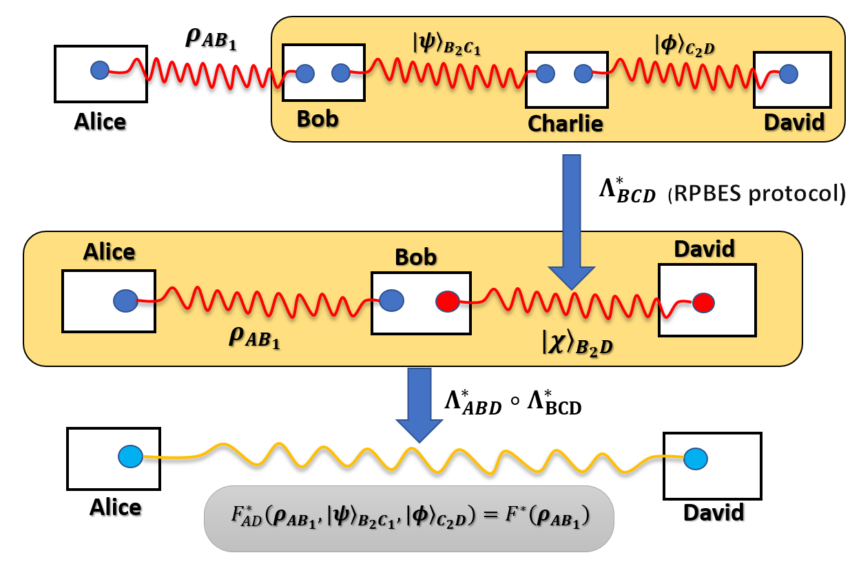
Figure 6: (Color online) An optimal four-party protocol for distributing teleportation channel between Alice and David, where only Alice-Bob share a noisy entangled state. As per the protocol, first Bob-Charlie-David collaborate and prepare best teleportation channel between Bob and David. Then Alice-Bob and David collaborate and optimally distribute the best possible channel between Alice-David. Although the preshared teleportation channels of $\mathcal{BC}$ and $\mathcal{CD}$ are noisy, on average they show the same advantage as a noiseless teleportation channel.

VI Discussion

In this present work, we have considered a network of three spatially separated parties, say, Alice, Bob, and Charlie. Here both $\mathcal{AB}$ and $\mathcal{BC}$ initially share a two-qubit state each, and all of them can perform LOCC. Our goal is to deterministically prepare a two-qubit state between $\mathcal{AC}$ via LOCC (collaboration) that possesses FEF which is optimized over three-party TP LOCC. We call this the optimally prepared teleportation channel under collaboration. The study becomes trivial if both the preshared states possess one ebit of entanglement. Then we know the only optimal protocol is the standard teleportation protocol, where Bob teleports one of his qubit through the noiseless qubit teleportation channel (1 ebit entanglement) of either $\mathcal{AB}$ or $\mathcal{BC}$. Thereafter Alice-Charlie perform local unitary correction and prepare another noiseless channel.

Nontriviality arises when the preshared states are noisy. In such a case, it is difficult to figure out the optimal TP LOCC which distributes the best teleportation channel between Alice and Charlie. So we first proposed the necessary conditions that every three-party TP LOCC should satisfy while distributing any two-qubit state. We then proposed the possible upper bounds on the FEF of the distributed state. Luckily we have found the optimal protocols for some classes of preshared two-qubit states. While studying the optimal protocols we have pointed out that the optimal distribution of teleportation channel has no correspondence with the optimal distribution of entanglement. For example, let $\mathcal{AB}$ share some noisy entangled state. Here one will argue that if $\mathcal{BC}$ share less entanglement than one ebit, then the optimal FEF of collaboration would be poor. Generally, this is not the case and this indicates that optimal teleportation of collaboration has no correspondence with optimal distribution of entanglement.

Our study has shown that for specific classes of preshared entangled states, one-way Bob-assisted TP LOCC protocols are sufficient to obtain the optimal FEF of collaboration. In the suboptimal cases i.e., where we cannot say that Bob-assisted protocols are optimal, we can surely say that there are instances where Bob’s PVM-assisted protocols in any maximally entangled basis are not efficient. Thus for such a case, PVM in partially entangled states are special i.e., they have an operational advantage even if they are weakly entangling operations. We have also observed that the efficient distribution of entanglement not necessarily implies that Bob has to initiate the protocol via performing PVM in a maximally entangled basis. In this regard, the RPBES protocol introduced in Gour and Sanders (2004) is in general not an efficient protocol for entanglement distribution.

We have also studied the network beyond the three-party case and observed that with the increasing number of parties, the complexity of the problem grows. Here by complexity, we mean that the number of independent upper bounds may increase and there is no unique way of saturating one or more bounds just like in the three-party case. However, our study has some limitations. Even for the three-party case, we could not answer with full generality that for arbitrary preshared states, what should be the exact structure of the optimal protocol? Answering this question is difficult since it requires characterization of canonical form(s) of the resulting two-qubit states of $\mathcal{AC}$ under any transformation from the group $SL(2,\mathbb{C})\otimes SL(4,\mathbb{C})\otimes SL(2,\mathbb{C})$ – a study, we would like to pursue in the near future. There can be some open directions of our study. One can consider the preshared states of $\mathcal{AB}$ and $\mathcal{BC}$ to be of infinite dimensions, a two-mode Gaussian state for example. This is because Gaussian states are easy to prepare experimentally. Furthermore, in any network-based problem, the distribution of teleportation channel is only facet. There can be different figures of merit one can think of in such distribution problems, where each of the figures of merit comes from a physical task.

Appendix A Detail proof of Proposition 3

Proof.

Suppose we have a pair of two-qubit entangled states $(\rho_{AB_{1}},\sigma_{B_{2}C})$ shared between Alice-Bob and Bob-Charlie such that $\rho_{AB_{1}}=(\Lambda_{ADC}\otimes\mathbb{I})\ket{\psi}_{AB_{1}}\bra{\psi}$ and $\sigma_{B_{2}C}=\ket{\phi}_{B_{2}C}\bra{\phi}$. Here $\ket{\psi}_{AB_{1}}$ and $\ket{\phi}_{B_{2}C}$ have their Schmidt decomposition as,

$$\ket{\psi}_{AB_{1}} =\sqrt{\alpha_{0}}\ket{00}+\sqrt{\alpha_{1}}\ket{11},\quad\quad\quad\alpha_{0}\geq\alpha_{1}>0$$

$$=(A_{\alpha}\otimes\mathbb{I})\ket{\Phi_{0}},\quad\quad\text{where,}\quad A_{\alpha}=diag\{\sqrt{2\leavevmode\nobreak\ \alpha_{0}},\leavevmode\nobreak\ \sqrt{2\leavevmode\nobreak\ \alpha_{1}}\leavevmode\nobreak\ \}$$

$$\ket{\phi}_{B_{2}C} =\sqrt{\beta_{0}}\ket{00}+\sqrt{\beta_{1}}\ket{11},\quad\quad\quad\beta_{0}\geq\beta_{1}>0,$$

$$=(\mathbb{I}\otimes B_{\beta})\ket{\Phi_{0}},\quad\quad\text{where,}\quad B_{\beta}=diag\{\sqrt{2\leavevmode\nobreak\ \beta_{0}},\leavevmode\nobreak\ \sqrt{2\leavevmode\nobreak\ \eta_{1}}\},$$ (73)

where $A_{\alpha}^{\dagger}A_{\alpha}$ and $B_{\beta}^{\dagger}B_{\beta}$ in Eq.  (73) are trace non-increasing CP maps i.e. $A_{\alpha}^{\dagger}A_{\alpha}\leq\mathbb{I}$ and $B_{\beta}^{\dagger}B_{\beta}\leq\mathbb{I}$ acting on the Bell state $\ket{\Phi_{0}}$. So the composite four-qubit state can be expressed as

$$\eta_{AB_{1}B_{2}C} =(\Lambda_{ADC}\otimes\mathbb{I})\ket{\psi}_{AB_{1}}\bra{\psi}\otimes\ket{\phi}_{B_{2}C}\bra{\phi}$$

$$=\sum_{i=0}^{1}(K_{i,p}\otimes\mathbb{I})\ket{\psi}_{AB_{1}}\bra{\psi}(K_{i,p}^{\dagger}\otimes\mathbb{I})\otimes\ket{\phi}_{B_{2}C}\bra{\phi}$$

$$=\sum_{i=0}^{1}(K_{i}\leavevmode\nobreak\ A_{\alpha}\otimes\mathbb{I})\ket{\Phi_{0}}_{AB_{1}}\bra{\Phi_{0}}(A_{\alpha}^{\dagger}\leavevmode\nobreak\ K_{i}^{\dagger}\otimes\mathbb{I})\otimes(\mathbb{I}\otimes B_{\beta})\ket{\Phi_{0}}_{B_{2}C}\bra{\Phi_{0}}(\mathbb{I}\otimes B_{\beta}^{\dagger})$$

$$=\dfrac{1}{4}\sum_{k,l=0}^{3}\ket{\psi^{*}_{k}}_{B_{1}B_{2}}\bra{\psi^{*}_{l}}\otimes\sum_{i=0}^{1}(K_{i}\leavevmode\nobreak\ A_{\alpha}\otimes B_{\beta})\ket{\psi_{k}}_{AC}\bra{\psi_{l}}(A_{\alpha}^{\dagger}\leavevmode\nobreak\ K_{i}^{\dagger}\otimes B_{\beta}^{\dagger}),$$ (74)

where $\{\ket{\psi_{k}}\}$ forms any orthonormal set of basis and $*$ is the complex conjugate of the vectors. Thus if Bob performs measurement in the basis, $\{\ket{\psi^{*}_{j}}_{B_{1}B_{2}}\}$ then the corresponding prepared state between Alice-Charlie becomes

$$\rho_{AC,\psi_{i}} =\dfrac{1}{p_{i}}\leavevmode\nobreak\ Tr_{B}\left((\ket{\psi^{*}_{i}}_{B_{1}B_{2}}\bra{\psi^{*}_{i}}\otimes\mathbb{I})\eta_{AB_{1}B_{2}C}\right)$$

$$=\dfrac{1}{p_{i}}\leavevmode\nobreak\ \sum_{i=0}^{1}(K_{i}\leavevmode\nobreak\ A_{\alpha}\otimes B_{\beta})\ket{\psi_{i}}_{AC}\bra{\psi_{i}}(A_{\alpha}^{\dagger\leavevmode\nobreak\ }K_{i}^{\dagger}\otimes B_{\beta}^{\dagger})$$

$$=\dfrac{1}{p_{i}}\leavevmode\nobreak\ (\Lambda_{ADC}\otimes\mathbb{I})(A_{\alpha}\otimes B_{\beta})\ket{\psi_{i}}_{AC}\bra{\psi_{i}}(A_{\alpha}^{\dagger}\otimes B_{\beta}^{\dagger})$$

$$=(\Lambda_{ADC}\otimes\mathbb{I})\ket{\chi_{i}}_{AC}\bra{\chi_{i}},\quad\quad i=0,1,2,3,$$ (75)

where $\ket{\chi_{i}}_{AC}=\dfrac{1}{\sqrt{p_{i}}}(A_{\alpha}\otimes B_{\beta})\ket{\psi_{i}}_{AC}$ and $p_{i}=Tr\left((A_{\alpha}^{\dagger}A_{\alpha}\otimes B_{\beta}^{\dagger}B_{\beta})\ket{\psi_{i}}_{AC}\bra{\psi_{i}}\right)$ is the probability of obtaining the state $\rho_{AC,\psi_{i}}$.

Bob performs PVM:

Now let us assume that Bob first starts the protocol by performing a PVM in the following basis:

$$\ket{\eta_{0}}=\sqrt{\delta_{0}}\ket{00}+\sqrt{\delta_{1}}\ket{11},\quad\ket{\eta_{1}}=\sqrt{\delta_{1}}\ket{00}-\sqrt{\delta_{0}}\ket{11},$$

$$\ket{\eta_{2}}=\sqrt{\delta_{0}}\ket{01}+\sqrt{\delta_{1}}\ket{10},\quad\ket{\eta_{3}}=\sqrt{\delta_{1}}\ket{01}-\sqrt{\delta_{0}}\ket{10},$$ (76)

where $\delta_{0}\geq\delta_{1}>0$. Hence, one can express each of the state $\ket{\chi_{i}}_{AC}=\dfrac{1}{\sqrt{p_{i}}}(A_{\alpha}\otimes B_{\beta})\ket{\eta_{i}}_{AC}$ as

$$\ket{\chi_{0}}_{AC}=\dfrac{1}{\sqrt{p_{0}}}\left(\sqrt{\delta_{0}\alpha_{0}\beta_{0}}\ket{00}+\sqrt{\delta_{1}\alpha_{1}\beta_{1}}\ket{11}\right)=\sqrt{A_{0}}\ket{00}+\sqrt{A_{1}}\ket{11}$$

$$\ket{\chi_{1}}_{AC}=\dfrac{1}{\sqrt{p_{1}}}\left(\sqrt{\delta_{1}\alpha_{0}\beta_{0}}\ket{00}-\sqrt{\delta_{0}\alpha_{1}\beta_{1}}\ket{11}\right)=\sqrt{B_{0}}\ket{00}-\sqrt{B_{1}}\ket{11}$$

$$\ket{\chi_{2}}_{AC}=\dfrac{1}{\sqrt{p_{2}}}\left(\sqrt{\delta_{0}\alpha_{0}\beta_{1}}\ket{01}+\sqrt{\delta_{1}\alpha_{1}\beta_{0}}\ket{10}\right)=\sqrt{C_{0}}\ket{01}+\sqrt{C_{1}}\ket{10}$$

$$\ket{\chi_{3}}_{AC}=\dfrac{1}{\sqrt{p_{3}}}\left(\sqrt{\delta_{1}\alpha_{0}\beta_{1}}\ket{01}-\sqrt{\delta_{0}\alpha_{1}\beta_{0}}\ket{10}\right)=\sqrt{D_{0}}\ket{01}-\sqrt{D_{1}}\ket{10},$$ (77)

where $p_{i}$ is the normalization factor for every $i$ and $\{A_{i},\leavevmode\nobreak\ B_{i},\leavevmode\nobreak\ C_{i},\leavevmode\nobreak\ D_{i}\}$ are the Schmidt coefficients of $\{\ket{\chi_{i}}_{AC}\}$. Now from the knowledge of $\{\ket{\chi_{i}}_{AC}\}$, one can figure out the optimal FEF of every $\rho_{AC,\eta_{i}}$ as

$$F^{*}(\rho_{AC,\eta_{0}}) =\dfrac{1}{2}\left(1+2\leavevmode\nobreak\ \sqrt{A_{0}\leavevmode\nobreak\ A_{1}\leavevmode\nobreak\ (1-p)}-p\leavevmode\nobreak\ A_{1}\right),\quad\quad\text{if,}\quad\sqrt{A_{0}A_{1}(1-p)}\geq pA_{1},$$

$$F^{*}(\rho_{AC,\eta_{1}}) =\dfrac{1}{2}\left(1+2\leavevmode\nobreak\ \sqrt{B_{0}\leavevmode\nobreak\ B_{1}\leavevmode\nobreak\ (1-p)}-p\leavevmode\nobreak\ B_{1}\right),\quad\quad\text{if,}\quad\sqrt{B_{0}B_{1}(1-p)}\geq pB_{1},$$

and, (78)

$$F^{*}(\rho_{AC,\eta_{0}}) =\dfrac{1}{2}\left(1+A_{0}\leavevmode\nobreak\ \dfrac{1-p}{p}\right),\leavevmode\nobreak\ \leavevmode\nobreak\ \leavevmode\nobreak\ \leavevmode\nobreak\ \leavevmode\nobreak\ \leavevmode\nobreak\ \leavevmode\nobreak\ \leavevmode\nobreak\ \leavevmode\nobreak\ \leavevmode\nobreak\ \leavevmode\nobreak\ \leavevmode\nobreak\ \leavevmode\nobreak\ \leavevmode\nobreak\ \leavevmode\nobreak\ \leavevmode\nobreak\ \quad\quad\quad\quad\text{if,}\quad\sqrt{A_{0}A_{1}(1-p)}<pA_{1},$$

$$F^{*}(\rho_{AC,\eta_{1}}) =\dfrac{1}{2}\left(1+B_{0}\leavevmode\nobreak\ \dfrac{1-p}{p}\right),\leavevmode\nobreak\ \leavevmode\nobreak\ \leavevmode\nobreak\ \leavevmode\nobreak\ \leavevmode\nobreak\ \leavevmode\nobreak\ \leavevmode\nobreak\ \leavevmode\nobreak\ \leavevmode\nobreak\ \leavevmode\nobreak\ \leavevmode\nobreak\ \leavevmode\nobreak\ \leavevmode\nobreak\ \leavevmode\nobreak\ \leavevmode\nobreak\ \leavevmode\nobreak\ \quad\quad\quad\quad\text{if,}\quad\sqrt{B_{0}B_{1}(1-p)}<pB_{1},$$ (79)

whereas,

$$F^{*}(\rho_{AC,\eta_{2}}) =\dfrac{1}{2}\left(1+2\leavevmode\nobreak\ \sqrt{C_{0}\leavevmode\nobreak\ C_{1}\leavevmode\nobreak\ (1-p)}-p\leavevmode\nobreak\ C_{1}\right),\quad\quad\text{if,}\quad\sqrt{C_{0}C_{1}(1-p)}\geq pC_{1},$$

$$F^{*}(\rho_{AC,\eta_{3}}) =\dfrac{1}{2}\left(1+2\leavevmode\nobreak\ \sqrt{D_{0}\leavevmode\nobreak\ D_{1}\leavevmode\nobreak\ (1-p)}-p\leavevmode\nobreak\ D_{1}\right),\quad\quad\text{if,}\quad\sqrt{D_{0}D_{1}(1-p)}\geq pD_{1},$$

and, (80)

$$F^{*}(\rho_{AC,\eta_{2}}) =\dfrac{1}{2}\left(1+C_{0}\leavevmode\nobreak\ \dfrac{1-p}{p}\right),\leavevmode\nobreak\ \leavevmode\nobreak\ \leavevmode\nobreak\ \leavevmode\nobreak\ \leavevmode\nobreak\ \leavevmode\nobreak\ \leavevmode\nobreak\ \leavevmode\nobreak\ \leavevmode\nobreak\ \leavevmode\nobreak\ \leavevmode\nobreak\ \leavevmode\nobreak\ \leavevmode\nobreak\ \leavevmode\nobreak\ \leavevmode\nobreak\ \leavevmode\nobreak\ \quad\quad\quad\quad\text{if,}\quad\sqrt{C_{0}C_{1}(1-p)}<pC_{1},$$

$$F^{*}(\rho_{AC,\eta_{3}}) =\dfrac{1}{2}\left(1+D_{0}\leavevmode\nobreak\ \dfrac{1-p}{p}\right),\leavevmode\nobreak\ \leavevmode\nobreak\ \leavevmode\nobreak\ \leavevmode\nobreak\ \leavevmode\nobreak\ \leavevmode\nobreak\ \leavevmode\nobreak\ \leavevmode\nobreak\ \leavevmode\nobreak\ \leavevmode\nobreak\ \leavevmode\nobreak\ \leavevmode\nobreak\ \leavevmode\nobreak\ \leavevmode\nobreak\ \leavevmode\nobreak\ \leavevmode\nobreak\ \quad\quad\quad\quad\text{if,}\quad\sqrt{D_{0}D_{1}(1-p)}<pD_{1},$$ (81)

Now let us consider a particular domain where all four inequality conditions,

$$\quad\sqrt{A_{0}\leavevmode\nobreak\ A_{1}(1-p)}<p\leavevmode\nobreak\ A_{1}$$

$$\quad\sqrt{B_{0}\leavevmode\nobreak\ B_{1}(1-p)}<p\leavevmode\nobreak\ B_{1}$$

$$\quad\sqrt{C_{0}\leavevmode\nobreak\ C_{1}(1-p)}<p\leavevmode\nobreak\ C_{1}$$

$$\quad\sqrt{D_{0}\leavevmode\nobreak\ D_{1}(1-p)}<p\leavevmode\nobreak\ D_{1}$$

are simultaneously satisfied. From these inequality conditions, one can argue that the following inequality conditions should be satisfied,

$$(1-p)\leavevmode\nobreak\ \delta_{0}\leavevmode\nobreak\ \delta_{1}\leavevmode\nobreak\ \alpha_{0}\leavevmode\nobreak\ \alpha_{1}\leavevmode\nobreak\ \beta_{0}\leavevmode\nobreak\ \beta_{1}<p^{2}\leavevmode\nobreak\ \delta^{2}_{1}\leavevmode\nobreak\ \alpha^{2}_{1}\leavevmode\nobreak\ \beta^{2}_{1}\leq p^{2}\leavevmode\nobreak\ \delta^{2}_{0}\leavevmode\nobreak\ \alpha^{2}_{1}\leavevmode\nobreak\ \beta^{2}_{1}\leq p^{2}\leavevmode\nobreak\ \delta^{2}_{0}\leavevmode\nobreak\ \alpha^{2}_{1}\leavevmode\nobreak\ \beta^{2}_{0},$$ (82)

where note that ranges of $\alpha_{0},\leavevmode\nobreak\ \beta_{0},\leavevmode\nobreak\ \delta_{0}$ is given by $\dfrac{1}{2}\leq\alpha_{0},\leavevmode\nobreak\ \beta_{0},\leavevmode\nobreak\ \delta_{0}<1$. Now if one trivially choose $\alpha_{0}=\beta_{0}=\delta_{0}=\dfrac{1}{2}$, then for this case the inequality in Eq.  (82) will satisfy if the channel parameter $p$ is in the range, $\dfrac{\sqrt{5}-1}{2}<p<1$. Note that the more general restriction on the channel parameter $p$ is that

$$p>\dfrac{1}{2}\left[\sqrt{\dfrac{\alpha_{0}^{2}\leavevmode\nobreak\ \beta_{0}^{2}\leavevmode\nobreak\ \delta_{0}^{2}}{\alpha_{1}^{2}\leavevmode\nobreak\ \beta_{1}^{2}\leavevmode\nobreak\ \delta_{1}^{2}}+4\left(\dfrac{\alpha_{0}\leavevmode\nobreak\ \beta_{0}\leavevmode\nobreak\ \delta_{0}}{\alpha_{1}\leavevmode\nobreak\ \beta_{1}\leavevmode\nobreak\ \delta_{1}}\right)}-\dfrac{\alpha_{0}\leavevmode\nobreak\ \beta_{0}\leavevmode\nobreak\ \delta_{0}}{\alpha_{1}\leavevmode\nobreak\ \beta_{1}\leavevmode\nobreak\ \delta_{1}}\right]\geq\dfrac{\sqrt{5}-1}{2},$$ (83)

because of the fact that $\alpha_{0}\leavevmode\nobreak\ \beta_{0}\leavevmode\nobreak\ \delta_{0}\geq\alpha_{1}\leavevmode\nobreak\ \beta_{1}\leavevmode\nobreak\ \delta_{1}$ holds in general. So as per the range of the parameters of $\alpha_{0},\leavevmode\nobreak\ \beta_{0},\leavevmode\nobreak\ \delta_{0}$, let us first assume that $\alpha_{0}\geq\alpha_{1}$, whereas $\beta_{0}=\delta_{0}=\dfrac{1}{2}$. With this, one can easily find the domain of allowed $\alpha_{0}$ as

$$\dfrac{1}{2}\leq\alpha_{0}<\dfrac{p^{2}}{1-p+p^{2}},\quad\quad\quad\quad\text{while,}\quad\dfrac{\sqrt{5}-1}{2}<p<1.$$ (84)

Next, let us assume that another independent parameter $\beta_{0}$ satisfy $\beta_{0}\geq\beta_{1}$ while also assuming $\alpha_{0}\geq\alpha_{1}$ from the restricted domain of Eq.  (84). Whereas, we assume, $\delta_{0}=\delta_{1}=\dfrac{1}{2}$. For this case, one can easily find out the restriction on $\beta_{0}$ as

$$\dfrac{1}{2}\leq\beta_{0}<\dfrac{p^{2}\leavevmode\nobreak\ (1-\alpha_{0})}{p^{2}+\alpha_{0}\leavevmode\nobreak\ (1-p+p^{2})},\quad\quad\text{while,}\quad\dfrac{1}{2}\leq\alpha_{0}<\dfrac{p^{2}}{1-p+p^{2}},\quad\text{and,}\quad\dfrac{\sqrt{5}-1}{2}<p<1.$$ (85)

Similarly, assuming the general case, where $\delta_{0}\geq\delta_{1}$, one finds out the most general condition on the parameters as

$$\dfrac{1}{2}\leq\delta_{0}<\dfrac{p^{2}(1-\alpha_{0}-\beta_{0}+\alpha_{0}\beta_{0})}{\alpha_{0}\beta_{0}(1-p)+p^{2}(1-\alpha_{0}-\beta_{0}+\alpha_{0}\beta_{0})},$$ (86)

while $\alpha_{0}$ and $\beta_{0}$ satisfy Eq.  (84) and Eq.  (85). So while all these conditions hold, one can easily find out that the average FEF i.e.,

$$F^{*}_{AC,\{\eta_{i}\}} =\sum_{i=0}^{3}p_{i}\leavevmode\nobreak\ F^{*}(\rho_{AC,\eta_{i}})$$

$$=\dfrac{1}{2}+\dfrac{(1-p)}{2p}(p_{0}\leavevmode\nobreak\ A_{0}+p_{1}\leavevmode\nobreak\ A_{1}+p_{2}\leavevmode\nobreak\ A_{2}+p_{3}\leavevmode\nobreak\ A_{3})$$

$$=\dfrac{1}{2}\left[1+\alpha_{0}\leavevmode\nobreak\ \dfrac{(1-p)}{p}\right]=\min\{F^{*}(\rho_{AB_{1}}),F^{*}(\sigma_{B_{2}C})\}=F^{*}_{AC}(\rho,\leavevmode\nobreak\ \sigma),$$ (87)

which ends the proof of Proposition 3. A major point to be noted here is that the average optimal FEF in Eq.  (87) is hitting the LOCC upper bound $\min\{F^{*}(\rho_{AB_{1}}),F^{*}(\sigma_{B_{2}C})\}$ which means Eq.  (85) and $(\ref{b14})$ must obey the strict inequality condition, $F^{*}(\rho_{AB_{1}})<F^{*}(\sigma_{B_{2}C})$. This means that the following inequality must hold i.e.,

$$\dfrac{1}{2}\left[1+\alpha_{0}\leavevmode\nobreak\ \dfrac{(1-p)}{p}\right]<F^{*}(\sigma_{B_{2}C})=\dfrac{1+2\sqrt{\beta_{0}\leavevmode\nobreak\ (1-\beta_{0})}}{2}$$ (88)

if Eq.  (85) and $(\ref{b14})$ are satisfied. From Eq.  (88) one can find a domain of $\beta_{0}$ as

$$\dfrac{1}{2}\leq\beta_{0}<\dfrac{p^{2}\leavevmode\nobreak\ (1-\alpha_{0})}{p^{2}+\alpha_{0}\leavevmode\nobreak\ (1-p+p^{2})}<\dfrac{1}{2}\left[1+\sqrt{1-\dfrac{\alpha_{0}^{2}\leavevmode\nobreak\ (1-p)^{2}}{p^{2}}}\right],$$

which is consistent with Eq.  (85). Hence, this implies that both the ineqaulity conditions Eq.  (85) and $(\ref{b14})$ are physically consistent. ∎

Appendix B Detail proof of Proposition 4

Proof.

Let us assume that $\mathcal{AB}$ share a Bell-diagonal state, say $\rho_{AB_{1}}=\sum_{i}p_{i}\leavevmode\nobreak\ \ket{\Phi_{i}}_{AB}\bra{\Phi_{i}}$, whereas, $\mathcal{BC}$ share another Bell-diagonal state, say $\sigma_{B_{2}C}=\sum_{j}q_{j}\leavevmode\nobreak\ \ket{\Phi_{j}}_{BC}\bra{\Phi_{j}}$. Hence, the initial composite state $\eta_{AB_{1}B_{2}C}$ has the form,

$$\eta_{AB_{1}B_{2}C} =\sum_{i,j=0}^{3}p_{i}q_{j}\ket{\Phi_{i}\leavevmode\nobreak\ \Phi_{j}}_{AB_{1}B_{2}C}\bra{\Phi_{i}\leavevmode\nobreak\ \Phi_{j}}$$

$$=\sum_{i,j=0}^{3}A_{ij}\leavevmode\nobreak\ \ket{\Phi_{0}\leavevmode\nobreak\ \Phi_{0}}_{AB_{1}B_{2}C}\bra{\Phi_{0}\leavevmode\nobreak\ \Phi_{0}}\leavevmode\nobreak\ A_{ij}^{\dagger},$$ (89)

where $A_{ij}$ has the form,

$$A_{ij}\ket{\Phi_{0}\leavevmode\nobreak\ \Phi_{0}}_{AB_{1}B_{2}C} =\sqrt{p_{i}q_{j}}(\sigma_{i}\otimes\mathbb{I}\otimes\mathbb{I}\otimes\sigma_{j})\ket{\Phi_{0}\leavevmode\nobreak\ \Phi_{0}}_{AB_{1}B_{2}C}$$

$$=\sqrt{p_{i}q_{j}}\leavevmode\nobreak\ \ket{\Phi_{i}\leavevmode\nobreak\ \Phi_{j}}_{AB_{1}B_{2}C},$$ (90)

where $\sigma_{i}$ is the $i^{th}$ Pauli matrix. For any choice of complete orthonormal basis, say $\{\ket{\psi_{i}}\}$ one can express the following identity,

$$\ket{\Phi_{0}\leavevmode\nobreak\ \Phi_{0}}_{AB_{1}B_{2}C}=\dfrac{1}{2}\sum_{k=0}^{3}\ket{\psi^{*}_{k}}_{B_{1}B_{2}}\otimes\ket{\psi_{k}}_{AC},$$ (91)

where $\ket{\psi^{*}_{k}}$ is the complex conjugate of $\ket{\psi_{k}}$. So using the above identity one can again rewrite Eq.  (89) as

$$\eta_{AB_{1}B_{2}C} =\sum_{i,j=0}^{3}A_{ij}\leavevmode\nobreak\ \ket{\Phi_{0}\leavevmode\nobreak\ \Phi_{0}}_{AB_{1}B_{2}C}\bra{\Phi_{0}\leavevmode\nobreak\ \Phi_{0}}\leavevmode\nobreak\ A_{ij}^{\dagger}$$

$$=\dfrac{1}{2}\sum_{k,l=0}^{3}\ket{\psi^{*}_{k}}_{B_{1}B_{2}}\bra{\psi^{*}_{l}}\otimes\sum_{i,j=0}^{3}B_{ij}\ket{\psi_{k}}_{AC}\bra{\psi_{l}}B_{ij}^{\dagger},$$ (92)

where $B_{ij}=\sqrt{p_{i}q_{j}}\leavevmode\nobreak\ \sigma_{i}\otimes\sigma_{j}$ is a separable Kraus operator on Alice and Charlie. Now consider two general Pauli channels, say $\Lambda_{p}$ and $\Lambda_{q}$ with Kraus operators $\{\sqrt{p_{i}}\leavevmode\nobreak\ \sigma_{i}\}$ and $\{\sqrt{q_{j}}\leavevmode\nobreak\ \sigma_{j}\}$ respectively. Therefore, Eq.  (92) can be modified as

$$\eta_{AB_{1}B_{2}C}=\dfrac{1}{2}\sum_{k,l=0}^{3}\ket{\psi^{*}_{k}}_{B_{1}B_{2}}\bra{\psi^{*}_{l}}\otimes(\Lambda_{p}\otimes\Lambda_{q})\ket{\psi_{k}}_{AC}\bra{\psi_{l}}$$ (93)

Bob starts with PVM:

Hence, doing projective measurement in $\{\ket{\psi^{*}_{k}}_{B_{1}B_{2}}\}$ basis will prepare the state between Alice-Charlie as

$$\rho_{AC}(\psi_{k})=(\Lambda_{p}\otimes\Lambda_{q})\ket{\psi_{k}}\bra{\psi_{k}}$$ (94)

with a probability $P_{k}=Tr\left[(\ket{\psi_{k}^{*}}_{B_{1}B_{2}}\bra{\psi_{k}^{*}}\otimes\mathbb{I})\eta_{AB_{1}B_{2}C}\right]=\frac{1}{4}$. Now, let us calculate the quantity known as the optimal pre-processed FEF as

$$F_{1}(\Lambda_{p},\Lambda_{q}) =\max_{\ket{\Phi}\in MES}\max_{\ket{\psi}}\bra{\Phi}(\Lambda_{p}\otimes\Lambda_{q})\rho_{\psi}\ket{\Phi},\quad\quad\text{where,}\quad\rho_{\psi}=\ket{\psi}\bra{\psi}$$

$$=\max_{\ket{\Phi}}\max_{\ket{\psi}}\sum_{i,j=0}^{3}p_{i}q_{j}\leavevmode\nobreak\ \bra{\Phi}(\sigma_{i}\otimes\sigma_{j})\rho_{\psi}(\sigma_{i}\otimes\sigma_{j})\ket{\Phi}$$

$$=\max_{\ket{\Phi}}\max_{\ket{\psi}}\sum_{i,j=0}^{3}p_{i}q_{j}\leavevmode\nobreak\ \bra{\psi}(\sigma_{i}\otimes\sigma_{j})\rho_{\Phi}(\sigma_{i}\otimes\sigma_{j})\ket{\psi}$$

$$=\max_{W}\max_{\ket{\psi}}\sum_{i,j=0}^{3}p_{i}q_{j}\leavevmode\nobreak\ \bra{\psi}(\sigma_{i}\otimes\sigma_{j})(W\otimes\mathbb{I})\ket{\Phi_{0}}\bra{\Phi_{0}}(W^{\dagger}\otimes\mathbb{I})(\sigma_{i}\otimes\sigma_{j})\ket{\psi}$$

$$=\max_{W}\max_{\ket{\psi}}\sum_{i,j=0}^{3}p_{i}q_{j}\leavevmode\nobreak\ \bra{\psi}(\sigma_{i}\leavevmode\nobreak\ W\leavevmode\nobreak\ \sigma_{j}^{T}\otimes\mathbb{I})\rho_{\Phi_{0}}(\sigma_{j}^{*}W^{\dagger}\leavevmode\nobreak\ \sigma_{i}\otimes\mathbb{I})\ket{\psi}$$

$$=\max_{W}\max_{\ket{\psi}}\bra{\psi}(\Lambda_{p}\circ W\circ\tilde{\Lambda}_{q}\otimes\mathbb{I})\rho_{\Phi_{0}}\ket{\psi}$$

$$=\max_{W}\lambda_{max}\left[(\Lambda_{p,W,q}\otimes\mathbb{I})\rho_{\Phi_{0}}\right],$$ (95)

where $W$ is a unitary from $SU(2)$ and note that the concatenated channel $\Lambda_{p,W,q}=\Lambda_{p}\circ W\circ\Lambda_{q}$ is a unital channel for any choice of $W$. Hence, from the observation of Ref. Pal et al. (2014), one can conclude that the largest eigenvector of the state $(\Lambda_{p,W,q}\otimes\mathbb{I})\ket{\Phi_{0}}\bra{\Phi_{0}}$ which is $\ket{\psi}$ must be a MES. Note that since $\Lambda_{p,W,q}$ is unital, the state $(\Lambda_{p,W,q}\otimes\mathbb{I})\ket{\Phi_{0}}\bra{\Phi_{0}}$ can always be converted to a Bell-diagonal state using some product unitary operation $U\otimes V$ such that the largest eigenvector $\ket{\psi}=\ket{\Phi_{0}}$.

This implies, without any loss of generality, Bob can perform measurement in the standard Bell basis i.e., $\ket{\psi_{k}}=(\mathbb{I}\otimes\sigma_{k})\ket{\Phi_{0}}$, for $k=0,1,2,3$. Then after unitary corrections by Alice and Charlie, the post-measurement state of Alice-Charlie can be uniquely expressed as

$$\rho_{AC}(\Lambda_{p},\Lambda_{q})=\sum_{i=0}^{3}\lambda_{i}\ket{\Phi_{i}}\bra{\Phi_{i}},\quad\quad\lambda_{0}\geq\lambda_{1}\geq\lambda_{2}\geq\lambda_{3},$$ (96)

where $\lambda_{0}=\max_{W}\leavevmode\nobreak\ \lambda_{max}\left[(\Lambda_{p,W,q}\otimes\mathbb{I})\rho_{\Phi_{0}}\right]=\lambda_{max}\left[(\Lambda_{p}\circ\Lambda_{q}^{T}\otimes\mathbb{I})\rho_{\Phi_{0}}\right]$ is the largest eigenvalue of $\rho_{AC}(\Lambda_{p},\Lambda_{q})$. Therefore, for every outcome $k$ the optimally pre-processed FEF between Alice and Charlie is

$$F_{1}(\Lambda_{p},\Lambda_{q})=\lambda_{max}\left[(\Lambda_{p}\circ\Lambda_{q}^{T}\otimes\mathbb{I})\rho_{\Phi_{0}}\right],\quad\quad\forall\leavevmode\nobreak\ k$$ (97)

So under the TP LOCC protocol where Bob starts with PVM, the best possible average FEF between Alice-Charlie can be expressed as

$$F^{*}_{AC}(\rho,\leavevmode\nobreak\ \sigma) =\sum_{k}P_{k}\max_{\Gamma_{LOCC,k}}\max_{\ket{\psi_{k}}}F(\rho_{AC}(\psi_{k}))$$

$$=F(\rho_{AC}(\Lambda_{p},\Lambda_{q}))=\lambda_{max}\left[(\Lambda_{p}\circ\Lambda_{q}^{T}\otimes\mathbb{I})\rho_{\Phi_{0}}\right].$$ (98)

Bob starts with POVM:

Suppose Bob starts the protocol by performing an $N$ outcome POVM operation with elements $\{\pi_{i,B_{1}B_{2}}\}$ such that $\sum_{i=1}^{N}\pi_{i,B_{1}B_{2}}=\mathbb{I}$. Note that each of the elements can be expressed as

$$\pi_{i,B_{1}B_{2}}=\sum_{k=0}^{3}q_{i,k}\ket{\psi^{*}_{i,k}}\bra{\psi^{*}_{i,k}},\quad\quad\quad q_{i,k}\geq 0\quad\forall i,k,$$ (99)

where $\sum_{k}q_{i,k}\leq 1$ and $\{\ket{\psi_{i,k}^{*}}\}$ forms a complete set of orthonormal basis. Note that the representation in Eq.  (99) is not unique.

So if Bob measures in $\pi_{i,B_{1}B_{2}}$ then without any loss of generality, the post-measurement state between Alice-Charlie can be expressed directly from Eq.  (92) as

$$\rho_{AC}(\pi_{i}) =\dfrac{Tr_{B_{1}B_{2}}\left[(\sqrt{\pi_{i,B_{1}B_{2}}}\otimes\mathbb{I})\leavevmode\nobreak\ \eta_{AB_{1}B_{2}C}\leavevmode\nobreak\ (\sqrt{\pi_{i,B_{1}B_{2}}}\otimes\mathbb{I})^{\dagger}\right]}{Tr\left[(\pi_{i,B_{1}B_{2}}\otimes\mathbb{I})\eta_{AB_{1}B_{2}C}\right]}$$

$$=\dfrac{1}{Q_{i}}\sum_{k=0}^{3}q_{i,k}\leavevmode\nobreak\ (\Lambda_{p}\otimes\Lambda_{q})\ket{\psi_{i,k}}\bra{\psi_{i,k}},$$ (100)

where $\{\ket{\psi_{i,k}}\}$ forms an orthonormal complete basis set for every $i$ and $Q_{i}=Tr\left[(\pi_{i,B_{1}B_{2}}\otimes\mathbb{I})\eta_{AB_{1}B_{2}C}\right]=\sum_{k=0}^{3}q_{i,k}$ is the probability of the measurement outcome.

The optimal FEF for any two-qubit state is a LOCC monotone by definition and cannot increase under convex roof. Therefore, one can argue that

$$F^{*}(\rho_{AC,\pi_{i}})\leq\dfrac{1}{Q_{i}}\sum_{k=0}^{3}q_{i,k}\leavevmode\nobreak\ F^{*}\left[(\Lambda_{p}\otimes\Lambda_{q})\ket{\psi_{i,k}}\bra{\psi_{i,k}}\right]\leq\lambda_{max}\left[(\Lambda_{p}\circ\Lambda_{q}^{T}\otimes\mathbb{I})\rho_{\Phi_{0}}\right].$$

This is because each of the extreme points $\ket{\psi_{i,k}}$ of the convex mixture $\{q_{i,k},\ket{\psi_{i,k}}\}$ becomes optimal iff it is a MES. Hence, optimal POVM elements must be Bell diagonal unless it is PVM or full rank measurement.

Optimal protocol:

So the observations infer that the optimal TP LOCC protocol that sufficiently distributes the best possible teleportation channel is a one-way LOCC protocol from Bob to Alice-Charlie. Here Bob must perform PVM in the standard Bell basis. Then depending on the outcome Alice and Charlie perform unitary correction in Pauli basis and they end up with the state of Eq.  (96). ∎

Appendix C Detail proof of Proposition 6

Proof.

Let us assume $\rho_{AB_{1}}=(\Lambda_{ADC}\otimes\mathbb{I})|\Phi_{0}\rangle\langle\Phi_{0}|$ and $\sigma_{B_{2}C}=\lambda|\Phi_{0}\rangle\langle\Phi_{0}|+(1-\lambda)\frac{\mathbb{I}}{4}$. We know that $\sigma_{B_{2}C}$ is entangled if $\lambda>\frac{1}{3}$. One can express $\sigma_{B_{2}C}$ as mixtures of Bell basis,

$$\sigma_{B_{2}C} =\lambda\leavevmode\nobreak\ |\Phi_{0}\rangle\langle\Phi_{0}|+(1-\lambda)\leavevmode\nobreak\ \dfrac{\mathbb{I}}{4}$$

$$=\left(\dfrac{1+3\lambda}{4}\right)|\Phi_{0}\rangle\langle\Phi_{0}|+\dfrac{1-\lambda}{4}\sum_{i=1}^{3}|\Phi_{i}\rangle\langle\Phi_{i}|$$

$$=F\leavevmode\nobreak\ |\Phi_{0}\rangle\langle\Phi_{0}|+\dfrac{1-F}{3}\sum_{j=1}^{3}(\mathbb{I}\otimes\sigma_{j})|\Phi_{0}\rangle\langle\Phi_{0}|(\mathbb{I}\otimes\sigma_{j})$$

$$=(\mathbb{I}\otimes\Lambda_{dep})|\Phi_{0}\rangle\langle\Phi_{0}|,$$ (101)

where $\Lambda_{dep}$ is the depolarzing channel with Kraus operators $\{\sqrt{F}\leavevmode\nobreak\ \mathbb{I},\leavevmode\nobreak\ \sqrt{\frac{1-F}{3}}\leavevmode\nobreak\ \sigma_{1},\leavevmode\nobreak\ \sqrt{\frac{1-F}{3}}\leavevmode\nobreak\ \sigma_{2},\leavevmode\nobreak\ \sqrt{\frac{1-F}{3}}\leavevmode\nobreak\ \sigma_{3}\}$ respectively.

The composite four-qubit state $\eta_{AB_{1}B_{2}C}$ can be written as (see Eq.  (92)

$$\eta_{AB_{1}B_{2}C} =\rho_{AB_{1}}\otimes\sigma_{B_{2}C}$$

$$=\dfrac{1}{4}\sum_{k,l=0}^{3}\ket{\psi^{*}_{k}}_{B_{1}B_{2}}\bra{\psi^{*}_{l}}\otimes(\Lambda_{ADC}\otimes\Lambda_{dep})\ket{\psi_{k}}_{AC}\bra{\psi_{l}},$$ (102)

where both the set $\{\ket{\psi_{k}}\}$ and $\{\ket{\psi^{*}_{k}}\}$ form complete set of orthonormal basis.

Bob performs PVM in any MES:

Now suppose Bob performs PVM in any orthogonal MES basis with four basis elements, say $\{\ket{\Psi^{*}_{i}}\}$ for $i=0,1,2,3$, where each state $\ket{\Psi^{*}_{i}}$ can be written as

$$\ket{\Psi^{*}_{i}} =(U^{*}\otimes V^{*})\leavevmode\nobreak\ \ket{\Phi_{i}},\quad\quad(U^{*})^{\dagger}U^{*}=(V^{*})^{\dagger}V^{*}=\mathbb{I},\leavevmode\nobreak\ \leavevmode\nobreak\ i=0,1,2,3$$

$$=(U^{*}\otimes\mathbb{I})(\mathbb{I}\otimes V^{*}\sigma_{i})\ket{\Phi_{0}}$$

$$=(\mathbb{I}\otimes V^{*}\sigma_{i})(U^{*}\otimes\mathbb{I})\ket{\Phi_{0}}=(\mathbb{I}\otimes V^{*}\sigma_{i}(U^{*})^{T})\ket{\Phi_{0}}=(\mathbb{I}\otimes W^{*}_{i})\ket{\Phi_{0}},$$

where $W^{*}_{i}=V^{*}\sigma_{i}U^{\dagger}$ is again a unitary from $SU(2)$. Now since the vectors $\{\ket{\Phi^{*}_{i}}\}$ are orthogonal, hence,

$$\langle\Psi^{*}_{i}|\Psi^{*}_{j}\rangle=\bra{\Phi_{0}}(\mathbb{I}\otimes W_{i}^{T}W_{j}^{*})\ket{\Phi_{0}}=\dfrac{1}{2}Tr(W_{i}^{T}W_{j}^{*})=\delta_{ij}$$ (103)

must be satisfied. Thus Bob’s measurement in $\ket{\Psi^{*}_{i}}$ prepares a two-qubit state between Alice-Charlie as

$$\rho_{AC,\Psi_{i}} =\dfrac{1}{P_{i}}Tr_{B_{1}B_{2}}\left[(\ket{\Psi^{*}_{i}}_{B_{1}B_{2}}\bra{\Psi^{*}_{i}}\otimes\mathbb{I})\eta_{AB_{1}B_{2}C}\right],\quad\quad i=0,1,2,3$$

$$=(\Lambda_{ADC}\otimes\Lambda_{dep})|\Psi_{i}\rangle\langle\Psi_{i}|$$

$$=(\Lambda_{ADC}\otimes\mathbb{I})\left[F\leavevmode\nobreak\ |\Psi_{i}\rangle\langle\Psi_{i}|+\frac{1-F}{3}\sum_{j=1}^{3}(\mathbb{I}\otimes\sigma_{j})|\Psi_{i}\rangle\langle\Psi_{i}|(\mathbb{I}\otimes\sigma_{j})\right],$$ (104)

where note that $\{\ket{\Psi_{i}}\}$ forms an orthonormal basis set since their complex conjugates are assumed to be orthonormal. Now notice that for every $i=0,1,2,3$ the following four vectors

$$\ket{\Psi_{i}}=\ket{\tilde{\Psi}_{0,i}}=(\mathbb{I}\otimes\sigma_{0}\leavevmode\nobreak\ W_{i})\ket{\Phi_{0}},\quad\ket{\tilde{\Psi}_{j,i}}=(\mathbb{I}\otimes\sigma_{j})\leavevmode\nobreak\ \ket{\Psi_{i}}=(\mathbb{I}\otimes\sigma_{j}\leavevmode\nobreak\ W_{i})\ket{\Phi_{0}}\quad\quad j=1,2,3$$

are orthogonal because the following condition

$$\langle\tilde{\Psi}_{k,i}|\tilde{\Psi}_{l,i}\rangle=\bra{\Phi_{0}}(\mathbb{I}\otimes W_{i}^{\dagger}\leavevmode\nobreak\ \sigma_{k}\leavevmode\nobreak\ \sigma_{l}\leavevmode\nobreak\ W_{i})\ket{\Phi_{0}}=\dfrac{1}{2}Tr\left(W_{i}^{\dagger}\leavevmode\nobreak\ \sigma_{k}\leavevmode\nobreak\ \sigma_{l}\leavevmode\nobreak\ W_{i}\right)=\delta_{kl}\quad\quad k,l=0,1,2,3$$

is always satisfied. So without any loss of generality $\rho_{AC,\Psi_{i}}$ can be modified as

$$\rho_{AC,\Psi_{i}}=(\Lambda_{ADC}\otimes\mathbb{I})\left[F\leavevmode\nobreak\ |\tilde{\Psi}_{0,i}\rangle\langle\tilde{\Psi}_{0,i}|+\frac{1-F}{3}\sum_{j=1}^{3}|\tilde{\Psi}_{j,i}\rangle\langle\tilde{\Psi}_{j,i}|\right],\quad\quad\langle\tilde{\Psi}_{k,i}|\tilde{\Psi}_{l,i}\rangle=\delta_{kl}\quad and\leavevmode\nobreak\ \leavevmode\nobreak\ k,l=0,1,2,3$$

Now again notice that for every $i=0,1,2,3$ the following four vectors,

$$\ket{\Phi_{0}}=\ket{\tilde{\Phi}_{0,i}}=(\mathbb{I}\otimes W_{i}^{\dagger})\ket{\tilde{\Psi}_{0,i}},\quad\quad\ket{\tilde{\Phi}_{j,i}}=(\mathbb{I}\otimes W_{i}^{\dagger})\ket{\tilde{\Psi}_{j,i}}\quad\quad j=1,2,3$$

are again orthogonal to each other because of the simple fact that

$$\langle\tilde{\Phi}_{k,i}|\tilde{\Phi}_{l,i}\rangle=\langle\tilde{\Psi}_{k,i}|\tilde{\Psi}_{l,i}\rangle=\delta_{kl}.$$ (105)

Hence, without any loss of generality, the state $\rho_{AC,\Psi_{i}}$ can be written as

$$\rho_{AC,\Psi_{i}} =(\Lambda_{ADC}\otimes\mathbb{I})(\mathbb{I}\otimes W_{i})\left[F\leavevmode\nobreak\ |\Phi_{0}\rangle\langle\Phi_{0}|+\dfrac{1-F}{3}\sum_{j=1}^{3}|\tilde{\Phi}_{j,i}\rangle\langle\tilde{\Phi}_{j,i}|\right](\mathbb{I}\otimes W_{i}^{\dagger})$$

$$=(\Lambda_{ADC}\otimes\mathbb{I})(\mathbb{I}\otimes W_{i})\left[\dfrac{4F-1}{3}|\Phi_{0}\rangle\langle\Phi_{0}|+\dfrac{1-F}{3}\mathbb{I}\right](\mathbb{I}\otimes W_{i}^{\dagger})$$

$$=(\Lambda_{ADC}\otimes\mathbb{I})(\mathbb{I}\otimes W_{i})\left[\lambda|\Phi_{0}\rangle\langle\Phi_{0}|+(1-\lambda)\dfrac{\mathbb{I}}{4}\right](\mathbb{I}\otimes W_{i}^{\dagger}).$$ (106)

So after unitary correction by Charlie via unitary $W_{i}^{\dagger}$, the modified state becomes independent of $i$ that is

$$(\mathbb{I}\otimes W_{i}^{\dagger})\leavevmode\nobreak\ \rho_{AC,\Psi_{i}}\leavevmode\nobreak\ (\mathbb{I}\otimes W_{i})=(\Lambda_{ADC}\otimes\mathbb{I})\left[\lambda|\Phi_{0}\rangle\langle\Phi_{0}|+(1-\lambda)\dfrac{\mathbb{I}}{4}\right].$$ (107)

So Eq.  (107) implies that even if Bob performs PVM in any complete set of MES, Charlie can suitably find an unitary for which Alice-Charlie always ends up with an unique state

$$\rho_{AC,\Phi_{0}} =(\Lambda_{ADC}\otimes\mathbb{I})\left[\lambda|\Phi_{0}\rangle\langle\Phi_{0}|+(1-\lambda)\dfrac{\mathbb{I}}{4}\right]$$

$$=(\Lambda_{ADC}\otimes\Lambda_{dep})|\Phi_{0}\rangle\langle\Phi_{0}|.$$ (108)

Therefore, one can argue that the average FEF after optimal post-processing by Alice-Charlie can be expressed as

$$F^{*}_{AC,\{\ket{\Psi_{i}}\}}=\dfrac{1}{4}\sum_{i=0}^{3}F^{*}(\rho_{AC,\Psi_{i}})=F^{*}(\rho_{AC,\Phi_{0}}).$$ (109)

Now let us fix the parameter $\lambda=\frac{2}{5}$ which implies that the preshared state $\sigma_{B_{2}C}$ is weakly entangled. So after fixing $\lambda$, one can evaluate $F^{*}(\rho_{AC,\Phi_{0}})$. For that one needs to solve the SDP (mentioned in Eq.  (9)) and by solving it, one can find the optimal feasible solutions,

$$F^{*}(\rho_{AC,\Phi_{0}}) =\left\{\begin{array}[]{cc}\dfrac{1}{20}\left(7+4\sqrt{1-p}-2p\right)>\dfrac{1}{2},&\quad\text{if,}\quad 0\leq p\leq\dfrac{1}{49}(4\sqrt{74}-29)\\ &\\ \dfrac{67+112\leavevmode\nobreak\ p+21\leavevmode\nobreak\ p^{2}}{40(3+7\leavevmode\nobreak\ p)}>\dfrac{1}{2},&\quad\text{if,}\quad\dfrac{1}{49}(4\sqrt{74}-29)<p<1/3\\ &\\ \dfrac{1}{2},&\quad\quad\text{if,}\quad\dfrac{1}{3}\leq p<1\end{array}\right.$$ (115)

Note that the solutions in Eq.  (115) are physically consistent because if one estimates the concurrence value of $\rho_{AC,\Phi_{0}}$, then one can find that

$$C(\rho_{AC,\Phi_{0}}) =\max\left\{0,\leavevmode\nobreak\ \leavevmode\nobreak\ \dfrac{1}{10}\sqrt{1-p}\left(\sqrt{9+21\leavevmode\nobreak\ p}-4\right)\right\},\quad\quad\text{for,}\quad 0\leq p<1$$

$$=\dfrac{1}{10}\sqrt{1-p}\left(\sqrt{9+21\leavevmode\nobreak\ p}-4\right)>0,\quad\quad\quad\quad\leavevmode\nobreak\ \leavevmode\nobreak\ \leavevmode\nobreak\ \leavevmode\nobreak\ \text{for,}\quad 0\leq p<1/3$$

$$=0,\quad\quad\quad\quad\quad\quad\leavevmode\nobreak\ \leavevmode\nobreak\ \leavevmode\nobreak\ \leavevmode\nobreak\ \leavevmode\nobreak\ \leavevmode\nobreak\ \leavevmode\nobreak\ \leavevmode\nobreak\ \leavevmode\nobreak\ \leavevmode\nobreak\ \leavevmode\nobreak\ \leavevmode\nobreak\ \leavevmode\nobreak\ \leavevmode\nobreak\ \leavevmode\nobreak\ \leavevmode\nobreak\ \leavevmode\nobreak\ \leavevmode\nobreak\ \leavevmode\nobreak\ \leavevmode\nobreak\ \leavevmode\nobreak\ \leavevmode\nobreak\ \leavevmode\nobreak\ \leavevmode\nobreak\ \leavevmode\nobreak\ \leavevmode\nobreak\ \leavevmode\nobreak\ \leavevmode\nobreak\ \leavevmode\nobreak\ \leavevmode\nobreak\ \leavevmode\nobreak\ \leavevmode\nobreak\ \leavevmode\nobreak\ \leavevmode\nobreak\ \leavevmode\nobreak\ \leavevmode\nobreak\ \leavevmode\nobreak\ \leavevmode\nobreak\ \leavevmode\nobreak\ \leavevmode\nobreak\ \leavevmode\nobreak\ \leavevmode\nobreak\ \leavevmode\nobreak\ \leavevmode\nobreak\ \text{for,}\quad\dfrac{1}{3}\leq p<1,$$ (116)

Since any $\rho_{AC,\Psi_{i}}$ is connected with $\rho_{AC,\Phi_{0}}$ via local unitary, the concurrence of $\rho_{AC,\Phi_{0}}$ is the average concurrence of the set $\{\rho_{AC,\Psi_{i}}\}$. So in the entire range of channel parameter $p$ i.e., $0\leq p<1$, one can find that $F^{*}(\rho_{AC,\Phi_{0}})$ is always upper bounded by

$$F^{*}(\rho_{AC,\Phi_{0}})\leq\dfrac{1+C(\rho_{AC,\Phi_{0}})}{2}$$

$$Thus,\quad\quad \dfrac{1}{4}\sum_{i=0}^{3}F^{*}(\rho_{AC,\Psi_{i}})\leq\dfrac{1+C(\rho_{AC,\Phi_{0}})}{2}=\dfrac{1}{4}\sum_{i=0}^{3}\dfrac{1+C(\rho_{AC,\Psi_{i}})}{2}$$ (117)

which is consistent in the entire range of $p\in[0,1)$.

Bob performs PVM in NMES:

Now let us consider that Bob performs PVM in some partially entangled basis, say,

$$\ket{\eta_{0}}=\frac{\sqrt{3}}{2}\ket{00}+\frac{1}{2}\ket{11},\quad\quad\ket{\eta_{1}}=\frac{1}{2}\ket{00}-\frac{\sqrt{3}}{2}\ket{11},$$

$$\ket{\eta_{2}}=\frac{\sqrt{3}}{2}\ket{01}+\frac{1}{2}\ket{10},\quad\quad\ket{\eta_{3}}=\frac{1}{2}\ket{01}-\frac{\sqrt{3}}{2}\ket{10}.$$

So in this case, the prepared state between Alice-Charlie becomes (see Eq.  (102))

$$\rho_{AC,\eta_{i}}=(\Lambda_{ADC}\otimes\Lambda_{dep})|\eta_{i}\rangle\langle\eta_{i}|,\quad\quad i=0,1,2,3,$$ (118)

which occurs with probability $q_{i}=Tr\left[(\ket{\eta_{i}}_{B_{1}B_{2}}\bra{\eta_{i}}\otimes\mathbb{I})\leavevmode\nobreak\ \eta_{AB_{1}B_{2}C}\right]=\frac{1}{4}$. Although the average entanglement cost of such a basis is strictly less than the average cost of a MES basis. However, the interesting fact is that even if the cost is low, measurement in such a basis is more efficient for teleportation channel distribution than doing PVM in any MES, which means

$$F^{*}_{AC,\{\eta_{i}\}}=\sum_{i=0}^{3}q_{i}\leavevmode\nobreak\ F^{*}(\rho_{AC,\eta_{i}})>F^{*}(\rho_{AC,\Phi_{0}})$$ (119)

is satisfied for at least some values of $p$ and $\lambda$. We already have the feasible solutions (see Eq.  (115)) for $\lambda=\frac{2}{5}$ while Bob performs PVM in any MES. So again we fix $\lambda=\frac{2}{5}$ and again find the feasible solutions for $F^{*}_{AC,\{\eta_{i}\}}$ as

$$F^{*}(\rho_{AC,\eta_{0}})=F^{*}(\rho_{AC,\eta_{2}}) =\dfrac{21\leavevmode\nobreak\ p^{2}+238\leavevmode\nobreak\ p+381}{80(9+7p)}>\dfrac{1}{2},\quad\quad\quad\text{if,}\quad 0<p<1$$

whereas,

$$F^{*}(\rho_{AC,\eta_{1}})=F^{*}(\rho_{AC,\eta_{3}}) =\dfrac{1}{240}(127-63\leavevmode\nobreak\ p)>\dfrac{1}{2},\quad\quad\quad\quad\text{if,}\quad 0\leq p<\dfrac{1}{9}$$

$$=\dfrac{1}{2},\quad\quad\quad\quad\leavevmode\nobreak\ \leavevmode\nobreak\ \leavevmode\nobreak\ \leavevmode\nobreak\ \leavevmode\nobreak\ \leavevmode\nobreak\ \leavevmode\nobreak\ \leavevmode\nobreak\ \leavevmode\nobreak\ \leavevmode\nobreak\ \leavevmode\nobreak\ \leavevmode\nobreak\ \leavevmode\nobreak\ \leavevmode\nobreak\ \leavevmode\nobreak\ \leavevmode\nobreak\ \leavevmode\nobreak\ \leavevmode\nobreak\ \leavevmode\nobreak\ \leavevmode\nobreak\ \leavevmode\nobreak\ \leavevmode\nobreak\ \leavevmode\nobreak\ \leavevmode\nobreak\ \leavevmode\nobreak\ \leavevmode\nobreak\ \leavevmode\nobreak\ \text{if,}\quad\dfrac{1}{9}\leq p<1.$$ (120)

Note here that these solutions are consistent because each of them does not exceed the already established upper bound,

$$F^{*}(\rho_{AC,\eta_{i}})\leq\dfrac{1+C(\rho_{AC,\eta_{i}})}{2},\quad\quad\quad\quad\forall i\quad\text{and for,}\quad 0\leq p<1,$$

where $C(\rho_{AC,\eta_{i}})$ is the concurrence of the two-qubit state $\rho_{AC,\eta_{i}}$ and has the following expression,

$$C(\rho_{AC,\eta_{0}})=C(\rho_{AC,\eta_{2}})=\max\left\{0,\leavevmode\nobreak\ \leavevmode\nobreak\ \dfrac{1}{20}(\sqrt{7\leavevmode\nobreak\ p+9}-4)\sqrt{3(1-p)}\right\}$$

$$C(\rho_{AC,\eta_{1}})=C(\rho_{AC,\eta_{3}})=\max\left\{0,\leavevmode\nobreak\ \leavevmode\nobreak\ \dfrac{1}{20}(4-3\sqrt{7\leavevmode\nobreak\ p+1})\sqrt{3(1-p)}\right\},$$

for the entire range $0\leq p<1$. Therefore, within the range $\frac{1}{3}<p<1$, the average FEF has the expression

$$F^{*}_{AC,\{\eta_{i}\}} =\dfrac{1}{4}\sum_{i=0}^{3}F^{*}(\rho_{AC,\eta_{i}})$$

$$=\dfrac{1}{2}\left[F^{*}(\rho_{AC,\eta_{0}})+F^{*}(\rho_{AC,\eta_{1}})\right]$$

$$=\dfrac{1}{2}\left(\dfrac{21\leavevmode\nobreak\ p^{2}+238\leavevmode\nobreak\ p+381}{80(9+7p)}+\dfrac{1}{2}\right)>F^{*}(\rho_{AC,\Phi_{0}})$$ (121)

is satisfied if $p>\frac{1}{3}$. Thus Eq.  (121) shows that PVM in partially entangled states is more efficient than PVM in any choice of MES basis while optimizing FEF between Alice-Charlie.

Bob performs POVM:

Now let us consider that Bob performs a five-outcome POVM operation, where the POVM elements $\{\Pi_{i}\}$ are

$$\Pi_{i}=B_{i}^{\dagger}\leavevmode\nobreak\ B_{i} =\left[|\Phi_{i}\rangle\langle\Phi_{i}|\leavevmode\nobreak\ \left(\sqrt{A_{0}^{\dagger}A_{0}}\otimes\mathbb{I}\right)\right]^{\dagger}\left[|\Phi_{i}\rangle\langle\Phi_{i}|\leavevmode\nobreak\ \left(\sqrt{A_{0}^{\dagger}A_{0}}\otimes\mathbb{I}\right)\right],\quad\quad\quad\quad i=0,1,2,3$$

$$=\left(\sqrt{A_{0}^{\dagger}A_{0}}\otimes\mathbb{I}\right)|\Phi_{i}\rangle\langle\Phi_{i}|\left(\sqrt{A_{0}^{\dagger}A_{0}}\otimes\mathbb{I}\right)$$

$$\Pi_{4} =\mathbb{I}_{4}-\sum_{i=0}^{3}\left(\sqrt{A_{0}^{\dagger}A_{0}}\otimes\mathbb{I}\right)|\Phi_{i}\rangle\langle\Phi_{i}|\left(\sqrt{A_{0}^{\dagger}A_{0}}\otimes\mathbb{I}\right)$$

$$=\mathbb{I}_{4}-\left(A_{0}^{\dagger}A_{0}\otimes\mathbb{I}\right),$$ (122)

where $B_{i}$ is the $i^{th}$ Kraus operator and we have

$$A_{0}=\left(\begin{array}[]{cc}1&0\\ 0&\dfrac{\sqrt{1-p}}{p}\end{array}\right)$$ (125)

which is some operator. The important point here is that the operator $A_{0}^{\dagger}A_{0}$ must be positive and trace non-increasing, otherwise, the constructed POVM’s will not be physical. Therefore, the only region where $0<\Pi_{i}<\mathbb{I}_{4}$ holds is when $p$ belongs to the region $\frac{\sqrt{5}-1}{2}<p<1$.

After performing $\Pi_{i}$, the composite four-qubit state $\eta_{AB_{1}B_{2}C}$ can be written as

$$\rho_{AB_{1}B_{2}C,i} =\dfrac{(\mathbb{I}\otimes B_{i,B_{1}B_{2}}\otimes\mathbb{I})\leavevmode\nobreak\ \eta_{AB_{1}B_{2}C}\leavevmode\nobreak\ (\mathbb{I}\otimes B_{i,B_{1}B_{2}}^{\dagger}\otimes\mathbb{I})}{Tr\left[(\mathbb{I}\otimes\Pi_{i,B_{1}B_{2}}\otimes\mathbb{I})\leavevmode\nobreak\ \eta_{AB_{1}B_{2}C}\right]}$$

$$=\dfrac{1}{Q_{i}}\leavevmode\nobreak\ (\mathbb{I}\otimes B_{i,B_{1}B_{2}}\otimes\mathbb{I})\leavevmode\nobreak\ \left[(\Lambda_{ADC}\otimes\mathbb{I})P_{\Phi_{0},AB_{1}}\otimes(\mathbb{I}\otimes\Lambda_{dep})P_{\Phi_{0},B_{2}C}\right]\leavevmode\nobreak\ (\mathbb{I}\otimes B_{i,B_{1}B_{2}}^{\dagger}\otimes\mathbb{I})$$

$$=\dfrac{1}{Q_{i}}(\mathbb{I}\otimes P_{\Phi_{i},B_{1}B_{2}}\otimes\mathbb{I})\left[(\Lambda_{ADC}\otimes\mathbb{I})P_{\psi_{0},AB_{1}}\otimes(\mathbb{I}\otimes\Lambda_{dep})P_{\Phi_{0},B_{2}C}\right](\mathbb{I}\otimes P_{\Phi_{i},B_{1}B_{2}}\otimes\mathbb{I}),$$ (126)

where we write $B_{i,B_{1}B_{2}}=P_{\Phi_{i},B_{1}B_{2}}\leavevmode\nobreak\ (A_{0}\otimes\mathbb{I})$, where $P_{\Phi_{i}}=|\Phi_{i}\rangle\langle\Phi_{i}|$ is the projector on the standard Bell basis and $Q_{i}=Tr\left[(\mathbb{I}\otimes\Pi_{i,B_{1}B_{2}}\otimes\mathbb{I})\leavevmode\nobreak\ \eta_{AB_{1}B_{2}C}\right]$ is the probability of obtaining $\rho_{AB_{1}B_{2}C,i}$. In Eq.  (126) we have used an identity that

$$\left(\mathbb{I}\otimes\sqrt{A_{0}^{\dagger}A_{0}}\right)\ket{\Phi_{0}}_{AB_{1}}=\sqrt{q}\leavevmode\nobreak\ \ket{\psi_{0}}_{AB_{1}},$$

where $q=Tr\left[(A_{0}^{\dagger}A_{0}\otimes\mathbb{I})\leavevmode\nobreak\ P_{\Phi_{0}}\right]$ is a normalization factor and $\ket{\psi_{0}}_{AB_{1}}=\dfrac{1}{\sqrt{q}}\left(\ket{00}+\frac{\sqrt{1-p}}{p}\ket{11}\right)$.

Hence, by following Eq.  (126) one can express the post-measurement state between Alice-Charlie for the $i^{th}$ outcome as

$$\rho_{AC,\Pi_{i}}=\dfrac{1}{Q_{i}}\left[(\Lambda_{A_{0}}\otimes\Lambda_{dep})\leavevmode\nobreak\ P_{\Phi_{i},AC}\right]=\dfrac{1}{Q_{i}}\left[(\Lambda_{ADC}\otimes\Lambda_{dep})\leavevmode\nobreak\ P_{\psi_{0},AC}\right],$$ (127)

where $\Lambda_{A_{0}}$ is a trace-non increasing CP qubit map and its action on any qubit state $\rho$ is given by $\Lambda_{A_{0}}\leavevmode\nobreak\ (\rho)=\Lambda_{ADC}\leavevmode\nobreak\ (\sqrt{A_{0}^{\dagger}A_{0}}\leavevmode\nobreak\ \rho\leavevmode\nobreak\ \sqrt{A_{0}^{\dagger}A_{0}})$.

Again by solving SDP one can find that for $\frac{\sqrt{5}-1}{2}<p<1$ the average FEF and the average concurrence,

$$F^{*}_{AC,\{\Pi_{i}\}}=\sum_{i}Q_{i}\leavevmode\nobreak\ F^{*}(\rho_{AC,\Pi_{i}})>F^{*}(\rho_{AC,\Phi_{0}}),\quad\quad\text{and,}$$

$$C_{AC,\{\Pi_{i}\}}>C_{AC,\{\Psi_{i}\}},$$

satisfy the strict inequality conditions. Thus this shows that POVM operation can be more efficient than doing PVM in any MES basis for distribution of teleportation channel as well as entanglement. ∎

References

- Gour and Sanders (2004) G. Gour and B. C. Sanders, Phys. Rev. Lett. 93, 260501 (2004).
- Bennett et al. (1993) C. H. Bennett, G. Brassard, C. Crépeau, R. Jozsa, A. Peres, and W. K. Wootters, Phys. Rev. Lett. 70, 1895 (1993).
- Horodecki et al. (1999) M. Horodecki, P. Horodecki, and R. Horodecki, Phys. Rev. A 60, 1888 (1999).
- Horodecki et al. (1996) R. Horodecki, M. Horodecki, and P. Horodecki, Physics Letters A 222, 21 (1996).
- Badzia¸g et al. (2000) P. Badzia¸g, M. Horodecki, P. Horodecki, and R. Horodecki, Phys. Rev. A 62, 012311 (2000).
- Řeháček et al. (2001) J. Řeháček, Z. Hradil, J. Fiurášek, and i. c. v. Brukner, Phys. Rev. A 64, 060301 (2001).
- Siddhu and Smolin (2023) V. Siddhu and J. Smolin, Phys. Rev. A 108, 032617 (2023).
- Verstraete and Verschelde (2003) F. Verstraete and H. Verschelde, Phys. Rev. Lett. 90, 097901 (2003).
- Verstraete et al. (2001) F. Verstraete, J. Dehaene, and B. DeMoor, Phys. Rev. A 64, 010101 (2001).
- Sudha et al. (2020) Sudha, H. S. Karthik, R. Pal, K. S. Akhilesh, S. Ghosh, K. S. Mallesh, and A. R. Usha Devi, Phys. Rev. A 102, 052419 (2020).
- Pal and Bandyopadhyay (2018) R. Pal and S. Bandyopadhyay, Phys. Rev. A 97, 032322 (2018).
- Perseguers et al. (2008) S. Perseguers, J. I. Cirac, A. Acín, M. Lewenstein, and J. Wehr, Phys. Rev. A 77, 022308 (2008).
- Dür et al. (1999) W. Dür, H.-J. Briegel, J. I. Cirac, and P. Zoller, Phys. Rev. A 59, 169 (1999).
- Bose et al. (1998) S. Bose, V. Vedral, and P. L. Knight, Phys. Rev. A 57, 822 (1998).
- Zeilinger et al. (1997) A. Zeilinger, M. A. Horne, H. Weinfurter, and M. Żukowski, Phys. Rev. Lett. 78, 3031 (1997).
- Konrad et al. (2007) T. Konrad, F. de Melo, M. Tiersch, C. Kasztelan, A. Aragão, and A. Buchleitner, Nature Physics 4, 99 (2007).
- Song et al. (2014) W. Song, M. Yang, and Z.-L. Cao, Phys. Rev. A 89, 014303 (2014).
- Bergou et al. (2021) J. A. Bergou, D. Fields, M. Hillery, S. Santra, and V. S. Malinovsky, Phys. Rev. A 104, 022425 (2021).
- Briegel et al. (1998) H.-J. Briegel, W. Dür, J. I. Cirac, and P. Zoller, Phys. Rev. Lett. 81, 5932 (1998).
- Razavi et al. (2009) M. Razavi, M. Piani, and N. Lütkenhaus, Phys. Rev. A 80, 032301 (2009).
- Kłobus et al. (2012) W. Kłobus, W. Laskowski, M. Markiewicz, and A. Grudka, Phys. Rev. A 86, 020302 (2012).
- Meng et al. (2021) X. Meng, J. Gao, and S. Havlin, Phys. Rev. Lett. 126, 170501 (2021).
- Li et al. (2021) J.-Y. Li, X.-X. Fang, T. Zhang, G. N. M. Tabia, H. Lu, and Y.-C. Liang, Phys. Rev. Res. 3, 023045 (2021).
- Hermans et al. (2022) S. Hermans, M. Pompili, H. Beukers, S. Baier, J. Borregaard, and R. Hanson, Nature 605, 663 (2022).
- Modławska and Grudka (2008) J. Modławska and A. Grudka, Phys. Rev. A 78, 032321 (2008).
- Wootters (1998) W. K. Wootters, Phys. Rev. Lett. 80, 2245 (1998).
- Bandyopadhyay and Ghosh (2012) S. Bandyopadhyay and A. Ghosh, Phys. Rev. A 86, 020304 (2012).
- Pal et al. (2014) R. Pal, S. Bandyopadhyay, and S. Ghosh, Phys. Rev. A 90, 052304 (2014).
- Horodecki et al. (2009) R. Horodecki, P. Horodecki, M. Horodecki, and K. Horodecki, Rev. Mod. Phys. 81, 865 (2009).
- Verstraete and Verschelde (2002) F. Verstraete and H. Verschelde, Phys. Rev. A 66, 022307 (2002).