Yutaka Yoshida

Department of Current Legal Study, Faculty of Law, Meiji Gakuin University, Yokohama, 244-8539, Japan.

Euler transformation for multiple $q$-hypergeometric series from wall-crossing formula of $K$-theoretic vortex partition function

1 Introduction and summary

Dualities relate supersymmetric quantum theories, which typically have the same fixed point in the renormalization group flow. In the level of supersymmetric indices and also partition functions, a duality implies the agreement of supersymmetric indices of the dual pair. Combined with supersymmetric localization formula, the agreement of indices predicts many non-trivial identities between special functions. For example, in four dimensions, the equality between superconformal indices [4, 5] of a dual pair predicts a non-trivial identity between integrals of elliptic gamma functions.

In three dimensions, supersymmetric localization formulas for supersymmetric indices/partition functions [6, 7, 8, 9] of $U(N)$ gauge theories on a closed three manifold $M_{3}$ have a remarkable factorization into a pair of $K$-theoretic vortex partition functions [10, 11, 12, 13, 14, 15]:

$$Z_{M_{3}}=\sum Z_{1\text{-loop}}Z_{\rm vortex}Z_{\rm vortex},\qquad(M_{3}=S^{3}_{b},S^{1}\times S^{2})\,.$$ (1.1)

Here $Z_{\rm vortex}$ called the $K$-theoretic vortex partition function is the generating function of Witten indices of supersymmetric quantum mechanics (SQM) associated with handsaw quiver of type $A_{1}$. Since a moduli space of vortex given by the Higgs branch vacua of SQM is isomorphic to a handsaw quiver of type $A_{1}$, the $K$-theoretic vortex partition function agrees with the generating function of an equivariant index such as the $\chi_{t}$-genus of handsaw quiver varieties of type $A_{1}$.

The problem to find the precise relation of $Z_{M_{3}}$’s between a three-dimensional (3d) Seiberg-like dual pair reduces to find the relation between the $K$-theoretic vortex partition functions of the Seiberg-like dual pair [16]. Later it is found [1] that the relation between the $K$-theoretic vortex partition functions of a Seiberg-like dual pair is the same as the wall-crossing (WC) formula of the $K$-theoretic vortex partition function with respect to the variation of the Fayet-Iliopoulos (FI) parameter of SQM.

In this article we will show that the wall-crossing formulas of vortex partition functions in 3d $\mathcal{N}=2$ and $\mathcal{N}=4$ $U(N)$ gauge theories obtained in [16, 1] are the same as Euler transformations of $q$-hypergeometric series studied by Kajihara [2], and Hallnäs, Langmann, Noumi and Rosengren [3], respectively. These Euler transformations are thought of as generalizations of Euler transformation of Gauss hypergeometric series:

$${}_{2}F_{1}(a,b;c;z)=(1-z)^{c-a-b}{}_{2}F_{1}(c-a,c-b;c;z)\,.$$ (1.2)

Since the $K$-theoretic vortex partition functions are the indices for handsaw quiver varieties, wall-crossing formulas give geometric interpretations of Euler transformations of $q$-hypergeometric series.

This article is organized as follows. In section 2.1, we review the $K$-theoretic vortex partition functions in 3d $\mathcal{N}=2$ Chern-Simons-matter theory (gauge theory with Chern-Simons term) and explain the relation between an ADHM-like description of the moduli space of vortices and a handsaw quiver variety of $A_{1}$. Then we obtain two distinct expressions of the supersymmetric localization formula in the positive and negative 1d FI-parameter region, respectively. In section 2.2, according to [1], we prove the wall-crossing formula which relates the vortex partition function in the positive FI-parameter and the one in the negative FI-parameter. In section 2.3 we give the precise parameter identification of the vortex partition function and Kajihara transformation.

We perform a similar computation in a 3d $\mathcal{N}=4$ gauge theory in section 3. In section 3.1, we review the $K$-theoretic vortex partition function for the 3d $\mathcal{N}=4$ theory. In section 3.2, we show that the wall-crossing formula of the vortex partition function agrees with a transformation formula [3] of trigonometric type. Next we explain the geometric interpretation of the vortex partition functions in section 3.3. For 3d $\mathcal{N}=4$ gauge theory, we find that the $K$-theoretic vortex partition function is the same as the equivariant $\chi_{t}$-genus up to a trivial factor. For 3d $\mathcal{N}=2$ gauge theory, although the $K$-theoretic $k$-vortex partition function and an index are related to each other up to some factor, the generating functions are different. We give a brief comment on an elliptic analogue of the wall-crossing formula in section 3.4.

In section 4, we perform the dimensional reduction from three dimensions to two dimension, and derive the wall-crossing formula of vortex partition functions in 2d $\mathcal{N}=(2,2)$ and $\mathcal{N}=(2,2)^{*}$ gauge theory. In section 5, we give comments on future directions of this work.

2 Kajihara transformation as wall-crossing formula

In this section we will show that the wall-crossing formula of $K$-theoretic vortex partition derived in [1] is the same as the Kajihara transformation of multiple $q$-hypergeometric series [2].

2.1 $K$-theoretic vortex partition function and handsaw quiver variety

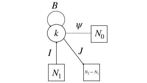
Figure 1: The quiver diagram representing 1d $\mathcal{N}=2$ SQM associated with the ADHM-like description of the $k$-vortex moduli for the 3d $\mathcal{N}=2$ gauge theory in Table 1. The circle with ’$k$’ denotes the 1d $\mathcal{N}=2$ $U(k)$ vector multiplet. An arrow with solid line denotes a 1d $\mathcal{N}=2$ chiral multiplet. The dashed line denotes the 1d $\mathcal{N}=2$ fermi multiplet. ’$I$’ and ’$J$’ denote the scalars in each chiral multiplet. ’$\psi$’ denotes the fermion in the fermi multiplet. The representation of the multiplets is summarized in Table 2

First, we review the vortex partition function of 3d $\mathcal{N}=2$ Chern-Simons-matter theory with the unitary the gauge group $U(N_{1})$ coupled to $N_{2}$ chiral multiplets in the fundamental representation of $U(N_{1})$ and with $N_{0}$ chiral multiplets in the anti-fundamental representation of $U(N_{1})$. In this paper, we assume $N_{0}\leq N_{2}$. The precise matter content of the 3d gauge theory is summarized in Table 1. As we will show the case for $N_{2}=N_{0}$ and zero Chern-Simons level: $\kappa=0$ is relevant to the Kajihara transformation.

Let us consider the partition function (supersymmetric index) of the 3d gauge theory on $S^{1}\times\mathbb{R}^{2}$ around the solutions of the vortex equation:

$$F_{12}=\frac{g^{2}}{2}(\phi\phi^{\dagger}-\xi 1_{N_{1}\times N_{1}}),$$

$$(D_{1}+{\rm i}D_{2})\phi=0\,.$$ (2.1)

with $k$-vortex number: $k=\frac{1}{2\pi}\int_{\mathbb{R}^{2}}\mathrm{Tr}F_{12}$. Here $F_{\mu\nu}=\partial_{\mu}A_{\nu}-\partial_{\nu}A_{\mu}+{\rm i}[A_{\mu},A_{\nu}]$ is the field strength of the $U(N_{1})$ gauge field $\{A_{\mu}\}_{\mu=0}^{2}$. $D_{\mu}=\partial_{\mu}+{\rm i}A_{\mu}$ is the covariant derivative. The suffix $\mu=1,2$ denotes the space-time directions along $\mathbb{R}^{2}$. As explained in Table 1, $\phi$ is the $N_{2}$-tuple scalars in the fundamental representation of the gauge group $U(N_{1})$. $\xi$ is the FI-parameter for the 3d gauge theory. Since the moduli data of the vortex equation has an ADHM-like description in terms of the D-brane construction [17] and the field theoretic construction [18, 19], the partition function of 3d gauge theory around the $k$-vortex background on $S^{1}\times\mathbb{R}^{2}$ reduces to the Witten index of 1d $\mathcal{N}=2$ SQM on $S^{1}$ associated with the handsaw quiver of type $A{}_{1}$ depicted by the Figure 1. The matter content of the SQM is depicted by Table 2.

In the SQM, the moduli space of the Higgs branch vacua is given by a Kähler quotient which is isomorphic to a handsaw quiver variety of type $A_{1}$:

$$\mathcal{M}^{(\zeta)}_{k,N_{1},N_{2}} =\Bigl{\{}(B,I,J)\Big{|}[B,B^{\dagger}]+II^{\dagger}-J^{\dagger}J=\zeta 1_{k\times k}\Bigr{\}}\Big{/}U(k)\,,$$ (2.2)

$$\simeq\{(B,I,J)\}/GL(N,\mathbb{C})\,.$$ (2.3)

Here

$$B\in\mathrm{End}(V),\,\,I\in\mathrm{Hom}(W^{(1)},\,\,V),\,\,J\in\mathrm{Hom}(V,W^{(2)})$$ (2.4)

with $V\simeq\mathbb{C}^{k},W^{(1)}\simeq\mathbb{C}^{N_{1}}$ and $W^{(2)}\simeq\mathbb{C}^{N_{2}-N_{1}}$ are the vacuum expectation values of the scalars in 1d $\mathcal{N}=2$ chiral multiplets. In (2.2) and (2.3), $g\in U(k)$ or $GL(k,\mathbb{C})$ acts on $(B,I,J)$ as $(B,I,J)\mapsto(gBg^{-1},gI,Jg^{-1})$. The quotients in (2.2) and (2.3) denote the Kähler quotient and the quotient with a stability condition.

The positive and the negative FI-parameter regions in (2.2) correspond to two different stability conditions of the handsaw quiver variety, respectively. According to the D-brane construction [17] and the field theoretic construction [18, 19] of the vortex moduli, the moduli space of the Higgs branch vacua $\mathcal{M}^{(\zeta>0)}_{k,N_{1},N_{2}}$ is isomorphic to the moduli space of $k$-vortex solutions of (2.1).

The Witten index for the 1d $\mathcal{N}=2$ SQM depicted by the handsaw quiver of type $A_{1}$ is called the $K$-theoretic $k$-vortex partition function for the 3d $\mathcal{N}=2$ gauge theory. Since the Witten index is related to an (equivariant) index of the moduli space of Higgs branch vacua of the SQM, $K$-theoretic vortex partition functions give indices of the handsaw quiver variety. Note that the fermion $\psi$ in the fermi multiplet corresponds to a characteristic class integrated over the handsaw quiver variety. This situation is analogous to the instanton case: the Witten indices for SQM depicted by the ADHM (Jordan) quiver are called $K$-theoretic instanton partition [20, 21], which give indices of the instanton moduli spaces. We will explain the geometric interpretation of the vortex partition functions in section 3.3.

	$U(N_{0})$	$U(N_{1})$	$U(N_{2})$
$\phi$	${\bm{1}}$	${\bm{N}_{1}}$	$\overline{\bm{N}_{2}}$
$\tilde{\phi}$	${\bm{N}_{0}}$	$\overline{\bm{N}_{1}}$	${\bm{1}}$

Table 1: The representation of the scalars in the 3d $\mathcal{N}=2$ chiral multiplets. $G=U(N_{1})$ is the gauge group of the 3d theory. $G_{F}=(U(N_{0})\times U(N_{2}))/U(1)$ is the flavor symmetry group. $U(1)_{R}$ is the R-symmetry group. Here $\phi\in\mathrm{Hom}(\mathbb{C}^{N_{1}},\mathbb{C}^{N_{2}})$ and $\tilde{\phi}\in\mathrm{Hom}(\mathbb{C}^{N_{0}},\mathbb{C}^{N_{1}})$ are the scalars in the chiral multiplets. ${\bm{N}_{s}}$, (resp. $\overline{\bm{N}_{s}}$) denotes the fundamental (resp. anti-fundamental) representation of $U(N_{s})$. ${\bm{1}}$ denotes the trivial representation.

	$U(k)$	$U(N_{1})$	$U(N_{2}-N_{1})$	$U(N_{0})$	$U(1)_{\varepsilon}$
$B$	$\bm{adj}$	${\bm{1}}$	${\bm{1}}$	${\bm{1}}$	$-1$
$I$	${\bm{k}}$	$\overline{\bm{N}_{1}}$	${\bm{1}}$	${\bm{1}}$	$-\frac{1}{2}$
$J$	$\bar{\bm{k}}$	${\bm{1}}$	${{\bm{N}_{2}}-{\bm{N}_{1}}}$	${\bm{1}}$	$-\frac{1}{2}$
$\psi$	$\bar{\bm{k}}$	${\bm{1}}$	${\bm{1}}$	${\bm{N}_{0}}$	$-\frac{1}{2}$

Table 2: The representation of the scalar and fermion in the 1d $\mathcal{N}=2$ multiplets describing $k$-vortex moduli in the 3d $\mathcal{N}=2$ $U(N_{1})$ gauge theory depicted by the quiver diagram in Figure 1 . The fields $B,I$ and $J$ are scalars in the 1d $\mathcal{N}=2$ chiral multiplets. A field $\psi$ is the fermion in the 1d $\mathcal{N}=2$ fermi multiplet. $U(k)$ is the gauge group. $U(N_{1})$, $U(N_{2}-N_{1})$ and $U(N_{0})$, as well as $U(1)_{\varepsilon}$ are the flavor symmetry group. ’$\bm{adj}$’ denotes the adjoint representation.

The $K$-theoretic $k$-vortex partition function $Z^{(\zeta)}_{k}$ is evaluated by applying the supersymmetric localization formula of the Witten index [21, 22]. Then we obtain the following residue integral expression

$$Z^{(\zeta)}_{k} =\frac{1}{k!(2\sinh\frac{-\varepsilon}{2})^{k}}\oint_{JK(\zeta)}\prod_{\alpha=1}^{k}\frac{du_{\alpha}}{2\pi{\rm i}}\prod_{1\leq\alpha\neq\beta\leq k}\frac{2\sinh\frac{u_{\alpha}-u_{\beta}}{2}}{2\sinh\frac{u_{\alpha}-u_{\beta}-\varepsilon}{2}}$$

$$\qquad\times\prod_{\alpha=1}^{k}\frac{e^{\kappa u_{\alpha}}\prod_{j=1}^{N_{0}}2\sinh\left({\frac{u_{\alpha}-\tilde{m}_{j}-\varepsilon/2}{2}}\right)}{\prod_{j=1}^{N_{1}}2\sinh\left(\frac{u_{\alpha}-m_{j}-\varepsilon/2}{2}\right)\cdot\prod_{j=N_{1}+1}^{N_{2}}2\sinh\left(\frac{-u_{\alpha}+m_{j}-\varepsilon/2}{2}\right)}\,.$$ (2.5)

In (2.5), complex parameters $\{m_{i}\}_{i=1}^{N_{1}}$, $\{m_{i}\}_{i=N_{1}+1}^{N_{2}}$ and $\{\tilde{m}_{i}\}_{i=1}^{N_{0}}$ are chemical potentials of 1d flavor symmetry groups $U(N_{1})$ $U(N_{2}-N_{1})$ and $U(N_{0})$ acting on $I,J$ and $\psi$, respectively. A chemical potential $\varepsilon$ is called an $\Omega$-background parameter.

Later $e^{m_{i}}$ and $e^{\varepsilon}$ are identified with the $(\mathbb{C}^{*})^{N_{2}+1}$-equivariant parameters associated with $U(N_{1})\times U(N_{2}-N_{1})\times U(1)_{\varepsilon}$-action on $\mathcal{M}^{(\zeta)}_{k,N_{1},N_{2}}$ defined by

$$(B,I,J)\mapsto(B,Ig^{-1}_{1},J),\quad g\in U(N_{1}),$$

$$(B,I,J)\mapsto(B,I,g_{2}J),\quad g_{2}\in U(N_{2}-N_{1}),$$ (2.6)

$$(B,I,J)\mapsto(g_{3}B,g_{3}I,g_{3}J),\quad g_{3}\in U(1)_{\varepsilon}\,.$$

$\kappa\in\mathbb{Z}$ or $\mathbb{Z}+\frac{1}{2}$ is the 1d Chern-Simons level induced by the 3d supersymmetric Chern-Simons term in the $U(N_{1})$ gauge theory:

$${S}_{CS} =\frac{\kappa}{4\pi{\rm i}}\int_{S^{1}\times\mathbb{R}^{2}}\mathrm{Tr}\left(A\wedge dA-\frac{2{\rm i}}{3}A^{3}\right)+\cdots\,.$$ (2.7)

The trace in (2.7) is taken for $\mathfrak{u}(N_{1})$. In this article we assume $-\frac{N_{2}-N_{0}}{2}\leq\kappa\leq\frac{N_{2}-N_{0}}{2}$ and $\kappa+\frac{N_{2}-N_{0}}{2}\in\mathbb{Z}$.

Let us evaluate the contour integral in (2.5). The contour is determined by the Jeffrey-Kirwan (JK) residues which correlated with the sign of the 1d FI-parameter $\zeta$ in the SQM [22]. The JK residues are evaluated as follows [1].

When the 1d FI parameter is positive $\zeta>0$, the JK residues in (2.5) are evaluated at the poles given by

$$u_{\alpha}-u_{\beta}-\varepsilon =0,\quad\alpha,\beta\in\{1,\cdots,k\},$$

$$u_{\alpha}-m_{i}-\frac{\varepsilon}{2} =0,\quad\alpha\in\{1,\cdots,k\},\,\,i\in\{1,\cdots,N_{1}\}.$$ (2.8)

Then the intersection points of the hyperplanes in (2.8) are classified as

$$u_{\alpha=\ell_{i}}=m_{i}+(\ell_{i}-1/2)\varepsilon,\quad\ell_{i}=1,\cdots,k_{i},\,\,\,i\in\{1,\cdots,N_{1}\},$$ (2.9)

where $k_{i}\geq 0$ and $\sum_{i=1}^{N_{1}}k_{i}=k$.

On the other hand, the JK residues in the negative FI-parameter region $\zeta<0$ are evaluated at

$$u_{\alpha}-u_{\beta}-\varepsilon =0,\quad\alpha,\beta\in\{1,\cdots,k\},$$

$$-u_{\alpha}+m_{j}-\frac{\varepsilon}{2} =0,\quad\alpha\in\{1,\cdots,k\},\,\,j\in\{N_{1}+1,\cdots N_{2}\}.$$ (2.10)

The intersection points of the hyperplanes in (2.10) are classified as

$$u_{\alpha=\ell_{i}}=m_{i}-(\ell_{i}-1/2)\varepsilon,\quad\ell_{i}=1,\cdots,k_{i},\,\,\,i\in\{N_{1}+1,\cdots,N_{2}\},$$ (2.11)

where $k_{i}\geq 0$ and $\sum_{i=N_{1}+1}^{N_{2}}k_{i}=k$. Then the $K$-theoretic $k$-vortex partition function in the positive and negative FI-parameter regions are given by

$$Z^{(\zeta>0)}_{k} =\sum_{k_{1}+\cdots+k_{N_{1}}=k}\frac{(-1)^{N_{1}k}e^{\kappa\sum_{i=1}^{N_{1}}(k_{i}m_{i}+k^{2}_{i}\varepsilon/2)}\prod_{i=1}^{N_{1}}\prod_{j=1}^{N_{0}}\prod_{\ell_{i}=1}^{k_{i}}2\sinh\left({\frac{m_{i}-\tilde{m}_{j}+(\ell_{i}-1)\varepsilon}{2}}\right)}{\prod_{i,j=1}^{N_{1}}\prod_{\ell_{i}=1}^{k_{i}}2\sinh\left(\frac{m_{j}-m_{i}-(\ell_{i}-k_{j}-1)\varepsilon}{2}\right)\prod_{i=1}^{N_{1}}\prod_{j=N_{1}+1}^{N_{2}}\prod_{\ell_{i}=1}^{k_{i}}2\sinh\left(\frac{-m_{i}+m_{j}-\ell_{i}\varepsilon}{2}\right)}$$ (2.12)

$$Z^{(\zeta<0)}_{k} =\sum_{{k}_{N_{1}+1}+\cdots+{k}_{N_{2}}={k}}\frac{(-1)^{(N_{2}-N_{1}+N_{0})k}e^{-\kappa\sum_{i=N_{1}+1}^{N_{2}}(-k_{i}m_{i}+k^{2}_{i}\varepsilon/2)}\prod_{i=N_{1}+1}^{N_{2}}\prod_{j=1}^{N_{0}}\prod_{\ell_{i}=1}^{k_{i}}2\sinh\left({\frac{-m_{i}+\tilde{m}_{j}+\ell_{i}\varepsilon}{2}}\right)}{\prod_{i,j=N_{1}+1}^{N_{2}}\prod_{\ell_{i}=1}^{k_{i}}2\sinh\left(\frac{-m_{j}+m_{i}-(\ell_{i}-k_{j}-1)\varepsilon}{2}\right)\prod_{i=N_{1}+1}^{N_{2}}\prod_{j=1}^{N_{1}}\prod_{\ell_{i}=1}^{k_{i}}2\sinh\left(\frac{m_{i}-m_{j}-\ell_{i}\varepsilon}{2}\right)}$$ (2.13)

Since the sign of the FI-parameter corresponds to the two distinct stability condition defining the handsaw quiver variety, the supersymmetric localization formula for the $K$-theoretic $k$-vortex partition functions (2.12) and (2.13) should be related to indices of handsaw quiver varieties with two different stability conditions. The vortex partition functions in the positive and negative FI-parameter regions possibly have different values: $Z^{(\zeta>0)}_{k}\neq Z^{(\zeta<0)}_{k}$, and such a situation is called a wall-crossing phenomenon.

2.2 Derivation of wall-crossing formula of vortex partition function

According to [1], we derive the relation between $Z^{(\zeta>0)}_{k}$ and $Z^{(\zeta<0)}_{k}$, i.e., the wall-crossing formula for $K$-theoretic vortex partition function, which is closely related to the wall-crossing formula for indices of handsaw quiver varieties of type $A_{1}$.

In order to derive the wall-crossing formula, first we introduce a multi-contour integral defined by

$$\mathcal{Z}_{k} :=\oint_{T^{k}_{x}}\frac{dx_{k}}{2\pi{\rm i}x_{k}}\cdots\frac{dx_{2}}{2\pi{\rm i}x_{2}}\frac{dx_{1}}{2\pi{\rm i}x_{1}}\mathcal{I}_{k}(x_{1},x_{2},\cdots x_{k})\,,$$ (2.14)

where

$$\mathcal{I}_{k}(x_{1},\cdots,x_{k}) =\frac{q^{\frac{k^{2}}{2}}}{k!(1-q)^{k}}(\prod_{i=1}^{N_{2}}x^{(2)}_{i})^{\frac{k}{2}}(\prod_{i=1}^{N_{0}}x^{(0)}_{i})^{-\frac{k}{2}}q^{\frac{(2N_{1}-N_{2}-N_{0})k}{4}}\prod_{1\leq\alpha\neq\beta\leq k}\frac{x_{\alpha}-x_{\beta}}{x_{\alpha}-qx_{\beta}}$$

$$\times\prod_{\alpha=1}^{k}\frac{x^{\kappa+\frac{N_{2}-N_{0}}{2}}_{\alpha}\prod_{j=1}^{N_{0}}(x_{\alpha}-x^{(0)}_{j}q^{\frac{1}{2}})}{\prod_{i=1}^{N_{1}}(x_{\alpha}-x^{(2)}_{i}q^{\frac{1}{2}})\cdot\prod_{j=N_{1}+1}^{N_{2}}(x^{(2)}_{j}q^{-\frac{1}{2}}-x_{\alpha})}\,.$$ (2.15)

Here ${T}^{k}_{x}$ is a $k$-dimensional torus defined by ${T}^{k}_{x}=\{(x_{1},\cdots,x_{k})\in\mathbb{C}^{k}||x_{1}|=\cdots=|x_{k}|=1\}$. We assume that the variables $q,x^{(2)}_{i}\in\mathbb{C}$ are in the following regions:

$$|q|<1,\,\,|x^{(2)}_{i}q^{n+\frac{1}{2}}|<1,\,\,|x^{(2)}_{j}q^{-n-\frac{1}{2}}|>1,$$ (2.16)

with $n=0,1,2,\cdots,$ $i=1,2,\cdots,N_{1},$ and $j=N_{1}+1,\cdots,N_{2}$.

The multi-contour integral in (2.14) is evaluated either by the residues inside the torus ${T}^{k}_{x}$, or by the residues outside of the torus. First we consider evaluating the residues inside the torus. In this case, the sequence of poles that contributing to the iterated residues are classified into the following two types. The first type includes at least one pole at the origin $x_{i}=0$ such that:

$$\{x_{i_{1}}=qx_{i_{2}},\,x_{i_{2}}=qx_{i_{3}},\,\cdots,x_{i_{n-1}}=qx_{i_{n}},\,x_{i_{n}}=0\}\,,$$

$$\{x_{i_{1}}=qx_{i_{3}},\,x_{i_{2}}=q^{2}x_{i_{3}},\,\cdots,x_{i_{n-1}}=qx_{i_{n}},\,x_{i_{n}}=0\}\,,$$

$$\cdots$$

$$\{x_{i_{1}}=0,\,x_{i_{2}}=0,\cdots,x_{i_{n-1}}=0,\,x_{i_{n}}=0\}\,.$$ (2.17)

Here $1\leq i_{1}<i_{2},<\cdots<i_{n}\leq k$ and $0\leq n\leq k$. The second type is given by the sequences of poles which do not include the pole at the origin:

$$\{x_{i_{n+1}}=qx_{i_{n+2}},\,x_{i_{n+2}}=qx_{i_{n+3}},\,\cdots,x_{i_{k-1}}=qx_{i_{k}},\,x_{i_{k}}=x^{(2)}_{j}q^{\frac{1}{2}}\},$$

$$\{x_{i_{n+1}}=qx_{i_{n+3}},\,x_{i_{n+2}}=q^{2}x_{i_{n+3}},\,\cdots,x_{i_{k-1}}=qx_{i_{k}},\,x_{i_{k}}=x^{(2)}_{j}q^{\frac{1}{2}}\},$$

$$\cdots$$

$$\{x_{i_{n+1}}=x^{(2)}_{j_{1}}q^{\frac{1}{2}},\,x_{i_{n+2}}=x^{(2)}_{j_{2}}q^{\frac{1}{2}},\cdots,x_{i_{k-1}}=x^{(2)}_{j_{k-n-1}}q^{\frac{1}{2}},\,x_{i_{k}}=x^{(2)}_{j_{k-n}}q^{\frac{1}{2}}\}.$$ (2.18)

Here $j_{1},\cdots j_{k-n}\in\{1,\cdots,N_{1}\}$. Except for the case where $\kappa=\frac{N_{2}-N_{0}}{2}$ is satisfied, the residues at the poles of the first type become zero. In this case, $\mathcal{Z}_{k}$ is given by the residues of the second type, which agrees with the $k$-vortex partition function (2.12). This is because that $\mathcal{I}_{k}(x_{1}\cdots,x_{k})$ is same as the integrand of (2.5) under the following identification of the parameters

$$x_{\alpha} =e^{u_{\alpha}},\,\,x^{(0)}_{a}=e^{\tilde{m}_{a}},\,\,x^{(2)}_{a}=e^{m_{a}},\,\,q=e^{\varepsilon},$$ (2.19)

and also that the second type poles are same as the poles (2.8) appeared in the JK residues operation under the identification (2.19).

On the other hand, the condition $\kappa=\frac{N_{2}-N_{0}}{2}$ is satisfied, residues at poles of the first type (2.17) are non-zero. The summation of the residues of the first type for $x_{i_{1}},\cdots,x_{i_{n}}$ is evaluated as follows. Since the second line in (2.15) is regular at the origin of $(x_{i_{1}},\cdots,x_{i_{n}})$, we may replace in the residue computation as

$$\prod_{\alpha\in\mathcal{J}}\prod_{\beta\in\mathcal{J}^{c}}\frac{x_{\alpha}-x_{\beta}}{x_{\alpha}-qx_{\beta}}\frac{x_{\beta}-x_{\alpha}}{x_{\beta}-qx_{\alpha}}\cdot\prod_{\alpha\in\mathcal{J}}\frac{x^{\kappa+\frac{N_{2}-N_{0}}{2}}_{\alpha}\prod_{j=1}^{N_{0}}(x_{\alpha}-x^{(0)}_{j}q^{\frac{1}{2}})}{\prod_{i=1}^{N_{1}}(x_{\alpha}-x^{(2)}_{i}q^{\frac{1}{2}})\cdot\prod_{j=N_{1}+1}^{N_{2}}(x^{(2)}_{j}q^{-\frac{1}{2}}-x_{\alpha})}$$

$$\underset{\{x_{i}=0\}_{i\in\mathcal{J}}}{\longrightarrow}(-1)^{N_{0}-N_{1}}q^{-2n(k-n)+(N_{0}+N_{2}-N_{1})\frac{n}{2}}(\prod_{a=1}^{N_{0}}x^{(0)}_{a})^{n}(\prod_{a=1}^{N_{2}}x^{(2)}_{a})^{-n}$$ (2.20)

Here $\mathcal{J}=\{i_{1},i_{2},\cdots,i_{n}\}$ and the set $\mathcal{J}^{c}$ is the complement of $\mathcal{J}$ in $\{1,\cdots,k\}$. Then the summation over the residues of $(x_{i_{1}},\cdots,x_{i_{n}})$ at the first type poles (2.17) is given by

$$\sum\underset{x_{i_{n}}}{\mathrm{Res}}\cdots\underset{x_{i_{1}}}{\mathrm{Res}}\,\frac{\mathcal{I}_{k}(x_{1},\cdots,x_{k})}{\prod_{\alpha=1}^{k}x_{\alpha}}$$

$$=\frac{n!(k-n)!}{k!}(-1)^{(N_{1}-N_{0})n}(\prod_{a=1}^{N_{0}}x^{(0)}_{a})^{\frac{n}{2}}(\prod_{a=1}^{N_{2}}x^{(2)}_{a})^{-\frac{n}{2}}q^{\frac{n}{4}(N_{0}+N_{2}-2N_{1})}\ \frac{\mathcal{I}_{k-n}(\{x_{i}\}_{i\in\mathcal{J}^{c}})}{\prod_{\alpha\in\mathcal{J}^{c}}x_{\alpha}}$$

$$\times\frac{q^{\frac{n^{2}}{2}}}{n!(1-q)^{n}}\oint_{T^{n}}\prod_{\alpha=1}^{n}\frac{dx_{i_{\alpha}}}{2\pi{\rm i}x_{i_{\alpha}}}\prod_{1\leq\alpha\neq\beta\leq n}\frac{x_{i_{\alpha}}-x_{i_{\beta}}}{x_{i_{\alpha}}-qx_{i_{\beta}}}$$

$$=\frac{n!(k-n)!}{k!}(-1)^{(N_{1}-N_{0})n}(\prod_{a=1}^{N_{0}}x^{(0)}_{a})^{\frac{n}{2}}(\prod_{a=1}^{N_{2}}x^{(2)}_{a})^{-\frac{n}{2}}q^{\frac{n}{4}(N_{0}+N_{2}-2N_{1})}\ \frac{\mathcal{I}_{k-n}(\{x_{i}\}_{i\in\mathcal{J}^{c}})}{\prod_{\alpha\in\mathcal{J}^{c}}x_{\alpha}}\frac{(-q^{\frac{1}{2}})^{n}}{(q;q)_{n}}$$ (2.21)

Here $(q;q)_{n}$ is a $q$-Pochhammer symbol defined by (A.4). In the last line in (2.21), we used the following formula:

$$\frac{q^{\frac{n^{2}}{2}}}{n!(1-q)^{n}}\sum\underset{x_{i_{n}}}{\mathrm{Res}}\cdots\underset{x_{i_{1}}}{\mathrm{Res}}\,\prod_{\alpha=1}^{n}x^{-1}_{i_{\alpha}}\cdot\prod_{1\leq\alpha\neq\beta\leq n}\frac{x_{i_{\alpha}}-x_{i_{\beta}}}{x_{i_{\alpha}}-qx_{i_{\beta}}}$$

$$=\frac{q^{\frac{n^{2}}{2}}}{n!(1-q)^{n}}\oint_{T^{n}_{x}}\prod_{\alpha=1}^{n}\frac{dx_{i_{\alpha}}}{2\pi{\rm i}x_{i_{\alpha}}}\prod_{1\leq\alpha\neq\beta\leq n}\frac{x_{i_{\alpha}}-x_{i_{\beta}}}{x_{i_{\alpha}}-qx_{i_{\beta}}}=\frac{(-q^{\frac{1}{2}})^{n}}{(q;q)_{n}}\,.$$ (2.22)

The iterated residues of the second type for $\{x_{i}\}_{\in\mathcal{J}^{c}}$ in the (2.21) gives $Z^{(\zeta>0)}_{n-k}$. By taking the summation over $1\leq i_{1}<\cdots<i_{n}\leq k$ and $n=0,1,\cdots,k$ , and taking all the possible residues at the first type poles for $\{x_{i}\}_{i\in\mathcal{J}}$ and also at the second type poles for $\{x_{i}\}_{i\in\mathcal{J}^{c}}$ give the relation between $\mathcal{Z}_{k}$ and $K$-theoretic vortex partition functions:

$$\mathcal{Z}_{k}=\left\{\begin{array}[]{cl}\sum\limits_{n=0}^{k}(-1)^{(N_{1}-N_{0})n}\left(\prod_{a=1}^{N_{0}}x^{(0)}_{a}\right)^{\frac{n}{2}}\left(\prod_{a=1}^{N_{2}}x^{(2)}_{a}\right)^{-\frac{n}{2}}q^{\frac{n}{4}(N_{0}+N_{2}-2N_{1})}\frac{(-q^{\frac{1}{2}})^{n}}{(q;q)_{n}}{Z}^{(\zeta>0)}_{k-n},&(\kappa=\frac{N_{0}-N_{2}}{2})\\ {Z}^{(\zeta>0)}_{k},&(\kappa\neq\frac{N_{0}-N_{2}}{2})\end{array}\right.$$ (2.25)

Next we consider evaluating the residues outside of the torus $T^{k}_{x}$. By changing the integration variables as $w_{i}=1/x_{i}$ for $i=1,\cdots,k$, the contour integral is evaluated by the residue inside of the torus $T^{k}_{w}$.

As in the case of the residues inside of $T^{k}_{x}$, the set of poles contributing to the residue for $w_{i}$ are classified into the following two types. The first one is given by

$$\{w_{i_{1}}=qw_{i_{2}},\,x_{i_{2}}=qw_{i_{3}},\,\cdots,w_{i_{n-1}}=qw_{i_{n}},\,w_{i_{n}}=0\}\,,$$

$$\{w_{i_{1}}=qw_{i_{3}},\,w_{i_{2}}=q^{2}w_{i_{3}},\,\cdots,w_{i_{n-1}}=qw_{i_{n}},\,w_{i_{n}}=0\}\,,$$

$$\cdots$$

$$\{w_{i_{1}}=0,\,w_{i_{2}}=0,\cdots,w_{i_{n-1}}=0,\,w_{i_{n}}=0\}\,.$$ (2.26)

The poles of second type are given by

$$\{w_{i_{n+1}}=qw_{i_{n+2}},\,w_{i_{n+2}}=qw_{i_{n+3}},\,\cdots,w_{i_{k-1}}=qw_{i_{k}},\,w_{i_{k}}=(x^{(2)}_{j})^{-1}q^{\frac{1}{2}}\},$$

$$\{w_{i_{n+1}}=qw_{i_{n+3}},\,w_{i_{n+2}}=q^{2}w_{i_{n+3}},\,\cdots,w_{i_{k-1}}=qw_{i_{k}},\,w_{i_{k}}=(x^{(2)}_{j})^{-1}q^{\frac{1}{2}}\},$$

$$\cdots$$

$$\{w_{i_{n+1}}=(x^{(2)}_{j_{1}})^{-1}q^{\frac{1}{2}},\,w_{i_{n+2}}=(x^{(2)}_{j_{1}})^{-1}q^{\frac{1}{2}},\cdots,w_{i_{k-1}}=(x^{(2)}_{j_{1}})^{-1}q^{\frac{1}{2}},\,w_{i_{k}}=(x^{(2)}_{j})^{-1}q^{\frac{1}{2}}\}.$$ (2.27)

Note that, if $-\frac{N_{2}-N_{0}}{2}\leq\kappa<\frac{N_{2}-N_{0}}{2}$, the residues at (2.26) are zero. In this case, the residues at (2.27) agrees with $Z^{(\zeta<0)}_{k}$ with the identification of the parameters (2.19). On the other hand, if $\kappa=\frac{N_{2}-N_{0}}{2}$ is satisfied, the residues at the first type poles gives non-zero contribution. In a similar way as (2.21), this residues can be calculated as follows.

$$\sum\underset{w_{i_{n}}}{\mathrm{Res}}\cdots\underset{w_{i_{1}}}{\mathrm{Res}}\frac{\mathcal{I}_{k}(w^{-1}_{1},\cdots,w^{-1}_{k})}{\prod_{\alpha=1}^{k}w_{\alpha}}$$

$$=\frac{n!(k-n)!}{k!}(-1)^{(N_{2}-N_{1})n}(\prod_{a=1}^{N_{0}}x^{(0)}_{a})^{-\frac{n}{2}}(\prod_{a=1}^{N_{2}}x^{(2)}_{a})^{\frac{n}{2}}q^{\frac{n}{4}(2N_{1}-N_{0}-N_{2})}\frac{\mathcal{I}_{k-n}(\{w^{-1}_{\alpha}\}_{\alpha\in\mathcal{J}^{c}})}{\prod_{\alpha\in\mathcal{J}^{c}}w^{-1}_{\alpha}}$$

$$\times\frac{q^{\frac{n^{2}}{2}}}{n!(1-q)^{n}}\oint_{T^{n}_{w}}\prod_{\alpha=1}^{n}\frac{dw_{i_{\alpha}}}{2\pi{\rm i}w_{i_{\alpha}}}\prod_{1\leq\alpha\neq\beta\leq n}\frac{w_{i_{\alpha}}-w_{i_{\beta}}}{w_{i_{\alpha}}-qw_{i_{\beta}}}$$

$$=\frac{n!(k-n)!}{k!}(-1)^{(N_{2}-N_{1})n}(\prod_{a=1}^{N_{0}}x^{(0)}_{a})^{-\frac{n}{2}}(\prod_{a=1}^{N_{2}}x^{(2)}_{a})^{\frac{n}{2}}q^{\frac{n}{4}(2N_{1}-N_{0}-N_{2})}\ \frac{\mathcal{I}_{k-n}(\{w^{-1}_{\alpha}\}_{\alpha\in\mathcal{J}^{c}})}{\prod_{\alpha\in\mathcal{J}^{c}}w^{-1}_{\alpha}}\frac{(-q^{\frac{1}{2}})^{n}}{(q;q)_{n}}\,.$$ (2.28)

We evaluate the residues at (2.27) and take the summation over all the poles in the first and the second type. Then we obtain

$$\mathcal{Z}_{k}=\left\{\begin{array}[]{cl}\sum\limits_{n=0}^{k}(-1)^{(N_{2}-N_{1})n}(\prod_{a=1}^{N_{0}}x^{(0)}_{a})^{-\frac{n}{2}}(\prod_{a=1}^{N_{2}}x^{(2)}_{a})^{\frac{n}{2}}q^{\frac{n}{4}(2N_{1}-N_{0}-N_{2})}\frac{(-q^{\frac{1}{2}})^{n}}{(q;q)_{n}}{Z}^{(\zeta<0)}_{k-n},&(\kappa=\frac{N_{2}-N_{0}}{2})\\ {Z}^{(\zeta<0)}_{k},&(\kappa\neq\frac{N_{2}-N_{0}}{2})\end{array}\right.$$ (2.31)

The equality of (2.25) and (2.31) gives the relation between $Z^{(\zeta>0)}_{k}$’s and $Z^{(\zeta<0)}_{k}$’s, i.e., the wall-crossing formula for the $K$-theoretic vortex partition functions.

In order to express the wall-crossing formula in a compact manner, we define a generating function of $k$-vortex partition functions by

$$Z^{(\zeta)}=1+\sum_{k=1}^{\infty}z^{k}Z^{(\zeta)}_{k}\,.$$ (2.32)

For simplicity we often refer to the generating function of vortex partition functions as the vortex partition function. Then the wall-crossing formula is expressed by

$$\sum_{k=0}^{\infty}z^{k}\mathcal{Z}_{k} =\left(\sum_{n=0}^{\infty}\frac{z^{n}_{+}}{(q;q)_{n}}\right)^{\delta_{2\kappa,N_{0}-N_{2}}}Z^{(\zeta>0)}$$

$$=\left(\sum_{n=0}^{\infty}\frac{z^{n}_{-}}{(q;q)_{n}}\right)^{\delta_{2\kappa,N_{2}-N_{0}}}Z^{(\zeta<0)}\,,$$ (2.33)

where $z_{+}$ and $z_{-}$ are defined by

$$z_{+} :=(-1)^{N_{1}-N_{0}+1}(\prod_{a=1}^{N_{0}}x^{(0)}_{a})^{\frac{1}{2}}(\prod_{a=1}^{N_{2}}x^{(2)}_{a})^{-\frac{1}{2}}q^{\frac{1}{4}(N_{0}+N_{2}-2N_{1}+2)}z\,,$$ (2.34)

$$z_{-} :=(-1)^{N_{1}-N_{2}+1}(\prod_{a=1}^{N_{0}}x^{(0)}_{a})^{-\frac{1}{2}}(\prod_{a=1}^{N_{2}}x^{(2)}_{a})^{\frac{1}{2}}q^{-\frac{1}{4}(N_{0}+N_{2}-2N_{1}-2)}z\,.$$ (2.35)

Using the $q$-binomial theorem (A.7), we obtain the following expression of the wall-crossing formula of the $K$-theoretic vortex partition function in 3d $\mathcal{N}=2$ gauge theory with the Chern-Simons term [1]:

$${(z_{+};q)_{\infty}^{{\delta_{2\kappa,N_{0}-N_{2}}}}}Z^{(\zeta>0)}={(z_{-};q)_{\infty}^{{\delta_{2\kappa,N_{2}-N_{0}}}}}\,Z^{(\zeta<0)}.$$ (2.36)

2.3 Kajihara transformation as WC formula in 3d $\mathcal{N}=2$ theory

Let us show that the wall-crossing formula (2.36) for $N_{2}=N_{0}$ and $\kappa=0$ is identical to the Kajihara transformation [2]. Using the identities (A.5) and (A.6), the $K$-theoretic vortex partition functions (2.12) and (2.13) with (2.19) are expressed as

$$Z^{(\zeta>0)} =\sum_{k=0}^{\infty}z_{+}^{k}\sum_{k_{1}+\cdots+k_{N_{1}}=k}\,\,\prod_{1\leq i<j\leq N_{1}}\frac{x^{(2)}_{i}q^{k_{i}}-x^{(2)}_{j}q^{k_{j}}}{x^{(2)}_{i}-x^{(2)}_{j}}$$

$$\qquad\times\prod_{i,j=1}^{N_{1}}\frac{(x^{(2)}_{i}/x^{(0)}_{j};q)_{k_{i}}}{(qx^{(2)}_{i}/x^{(2)}_{j};q)_{k_{i}}}\cdot\prod_{i=1}^{N_{1}}\prod_{j=N_{1}+1}^{N_{2}}\frac{(x^{(2)}_{i}/x^{(0)}_{j};q)_{k_{i}}}{(qx^{(2)}_{i}/x^{(2)}_{j};q)_{k_{i}}}\,,$$ (2.37)

$$Z^{(\zeta<0)} =\sum_{k=0}^{\infty}z_{-}^{{k}}\sum_{{k}_{N_{1}+1}+\cdots+{k}_{N_{2}}={k}}\,\,\prod_{N_{1}+1\leq i<j\leq N_{2}}\frac{(x^{(2)}_{i})^{-1}q^{{k}_{i}}-(x^{(2)}_{j})^{-1}q^{{k}_{j}}}{(x^{(2)}_{i})^{-1}-(x^{(2)}_{j})^{-1}}$$

$$\qquad\times\prod_{i,j=N_{1}+1}^{N_{2}}\frac{(qx^{(0)}_{i}/x^{(2)}_{j};q)_{{k}_{i}}}{(qx^{(2)}_{i}/x^{(2)}_{j};q)_{{k}_{i}}}\cdot\prod_{i=N_{1}+1}^{N_{2}}\prod_{j=1}^{N_{1}}\frac{(qx^{(0)}_{j}/x^{(2)}_{i};q)_{{k}_{i}}}{(qx^{(2)}_{j}/x^{(2)}_{i};q)_{{k}_{i}}}\,.$$ (2.38)

Next we define ${\sf x}_{i},{\sf y}_{i},{\sf a}_{i},{\sf b}_{i},{\sf c}$, and ${\sf z}$ by

$$x^{(2)}_{i} =\left\{\begin{array}[]{cl}\frac{{\sf x}_{i}}{{\sf x}_{N_{1}}},&i\in\{1,\cdots,N_{1}\}\,,\\ \frac{q\,{\sf y}_{N_{2}-N_{1}}}{c\,{\sf y}_{i-N_{1}}},&i\in\{N_{1}+1,\cdots,N_{2}\}\end{array}\right.$$ (2.41)

$$x^{(0)}_{i} =\left\{\begin{array}[]{cl}\frac{{\sf x}_{i}}{{\sf x}_{N_{1}}{\sf a}_{i}},&i\in\{1,\cdots,N_{1}\}\,,\\ \frac{{\sf y}_{N_{2}-N_{1}}}{{\sf b}_{i-N_{1}}\,{\sf y}_{i-N_{1}}}\,,&i\in\{N_{1}+1,\cdots,N_{2}\}\,,\end{array}\right.$$ (2.44)

$$(-1)^{N_{1}-N_{2}+1} (\prod_{a=1}^{N_{2}}x^{(0)}_{a}/x^{(2)}_{a})^{\frac{1}{2}}q^{\frac{1}{2}(N_{2}-N_{1}+1)}z=z_{+}={\sf z}\,.$$ (2.45)

Then the wall-crossing formula (2.36) is written as

$$\sum_{k=0}^{\infty}{\sf z}^{k}\sum_{k_{1}+\cdots+k_{N_{1}}=k}\prod_{1\leq i<j\leq N_{1}}\frac{{\sf x}_{i}q^{k_{i}}-{\sf x}_{j}q^{k_{j}}}{{\sf x}_{i}-{\sf x}_{j}}\cdot\prod_{i,j=1}^{N_{1}}\frac{({\sf a}_{j}{\sf x}_{i}/{\sf x}_{j};q)_{k_{i}}}{(q\,{\sf x}_{i}/{\sf x}_{j};q)_{k_{i}}}\cdot\prod_{i=1}^{N_{1}}\prod_{j=1}^{N_{2}-N_{1}}\frac{({\sf b}_{j}{\sf x}_{i}{\sf y}_{j}/{\sf x}_{N_{1}}{\sf y}_{N_{2}-N_{1}};q)_{k_{i}}}{(c{\sf x}_{i}{\sf y}_{j}/{\sf x}_{N_{1}}{\sf y}_{N_{2}-N_{1}};q)_{k_{i}}}$$

$$=\frac{({\sf z}\,c^{N_{2}-N_{1}}\prod_{i=1}^{N_{1}}{\sf a}_{i}\prod_{j=1}^{N_{2}-N_{1}}{\sf b}_{j};q)_{\infty}}{({\sf z};q)_{\infty}}\sum_{k=0}^{\infty}\Bigl{(}{\sf z}\,c^{N_{2}-N_{1}}\prod_{i=1}^{N_{1}}{\sf a}_{i}\prod_{j=1}^{N_{2}-N_{1}}{\sf b}_{j}\Bigr{)}^{{k}}\sum_{{k}_{1}+\cdots+{k}_{N_{2}-N_{1}}={k}}$$

$$\times\prod_{1\leq i<j\leq N_{2}-N_{1}}\frac{{\sf y}_{i}q^{{k}_{i}}-{\sf y}_{j}q^{k_{j}}}{{\sf y}_{i}-{\sf y}_{j}}\cdot\prod_{i,j=1}^{N_{2}-N_{1}}\frac{((c/{\sf b}_{j}){\sf y}_{i}/{\sf y}_{j};q)_{{k}_{i}}}{(q\,{\sf y}_{i}/{\sf y}_{j};q)_{{k}_{i}}}\cdot\prod_{i=1}^{N_{2}-N_{1}}\prod_{j=1}^{N_{1}}\frac{((c/{\sf a}_{j}){\sf y}_{i}{\sf x}_{j}/{\sf y}_{N_{2}-N_{1}}{\sf x}_{N_{1}};q)_{{k}_{i}}}{(c{\sf y}_{i}{\sf x}_{j}/{\sf y}_{N_{2}-N_{1}}{\sf x}_{N_{1}};q)_{{k}_{i}}}$$

This agrees with Kajihara transformation [2] of Kajihara-Noumi multiple hypergeometric series [23]. The wall-crossing formula for the general $N_{2},N_{0}$ and $\kappa$ is thought as a generalization of Kajihara transformation.

3 Hallnäs-Langmann-Noumi-Rosengren formula as wall-crossing formula

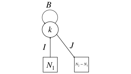
Figure 2: The quiver diagram representing the 1d $\mathcal{N}=4$ SQM associated with the $k$-vortex moduli for the 3d $\mathcal{N}=4$ gauge theory. The circle with ’$k$’ denotes the 1d $\mathcal{N}=4$ $U(k)$ vector multiplet. An arrow with solid line denotes a 1d $\mathcal{N}=4$ chiral multiplet. ’$B$’, ’$I$’ and ’$J$’ denote the scalars in each 1d $\mathcal{N}=4$ chiral multiplet. The representation of the 1d multiplets are the same as the 1d $\mathcal{N}=2$ case and summarized in Table 3

	$U(k)$	$U(N_{1})$	$U(N_{2}-N_{1})$	$U(N_{0})$	$U(1)_{\varepsilon}$
$B$	$\bm{adj}$	${\bm{1}}$	${\bm{1}}$	${\bm{1}}$	$-1$
$I$	${\bm{k}}$	$\overline{\bm{N}_{1}}$	${\bm{1}}$	${\bm{1}}$	$-\frac{1}{2}$
$J$	$\bar{\bm{k}}$	${\bm{1}}$	${{\bm{N}_{2}}-{\bm{N}_{1}}}$	${\bm{1}}$	$-\frac{1}{2}$

Table 3: The representation of the scalars in the 1d $\mathcal{N}=4$ chiral multiplets describing $k$-vortex moduli in the 3d $\mathcal{N}=4$ $U(N_{1})$ gauge theory depicted by the quiver diagram in Figure 2 . $B,I$ and $J$ are scalar in the chiral multiplets. $U(k)$ is the gauge group of the SQM. $U(N_{1})$, $U(N_{2}-N_{1})$ and $U(N_{0})$ $U(1)_{\varepsilon}$ are flavor symmetry groups.

In the previous section we have shown that the wall-crossing formula of vortex partition function in 3d $\mathcal{N}=2$ supersymmetric gauge theory agrees with the Kajihara transformation. In this section we will show that the wall-crossing formula of vortex partition function in 3d $\mathcal{N}=4$ $U(N_{1})$ supersymmetric gauge theory agrees with the trigonometric limit of transformation formula by Hallnäs-Langmann-Noumi-Rosengren formula [3]. The hypermultiplets in the $U(N_{1})$ gauge theory are the same as the chiral multiplets in Table 1 with $N_{0}=N_{2}$. The 3d $\mathcal{N}=4$ $U(N_{1})$ vector multiplet is given by 3d $\mathcal{N}=2$ with an additional chiral multiplet in the adjoint representation of $U(N_{1})$.

3.1 Vortex partition function in 3d $\mathcal{N}=4$ gauge theory

First we briefly review the $K$-theoretic vortex partition function in 3d $\mathcal{N}=4$ gauge theory. As explained in the section 2.1, the partition function of the $\mathcal{N}=2$ gauge theory on $S^{1}\times\mathbb{R}^{2}$ reduce to the $K$-theoretic vortex partition function given by the Witten index of 1d $\mathcal{N}=2$ SQM. Since the vortex equation is a half-BPS equation, the partition function of the 3d $\mathcal{N}=4$ $U(N_{1})$ gauge theory on $S^{1}\times\mathbb{R}^{2}$ reduce to the $K$-theoretic vortex partition function given by the Witten index of 1d $\mathcal{N}=4$ SQM depicted by the handsaw quiver in Figure 2.

From the supersymmetric localization formula, the $K$-theoretic $k$-vortex partition function of 3d $\mathcal{N}=4$ gauge theory is given by

$$Z^{(\zeta)}_{k,(N_{1},N_{2})} =\frac{1}{k!(2\sinh\frac{-m}{2})^{k}}\oint_{JK(\zeta)}\prod_{\alpha=1}^{k}\frac{du_{\alpha}}{2\pi{\rm i}}\left(\prod_{1\leq\alpha\neq\beta\leq k}\frac{2\sinh\frac{u_{\alpha}-u_{\beta}}{2}}{2\sinh\frac{u_{\alpha}-u_{\beta}-m}{2}}\right)\left(\prod_{\alpha,\beta=1}^{k}\frac{2\sinh\frac{u_{\alpha}-u_{\beta}-m-\varepsilon}{2}}{2\sinh\frac{u_{\alpha}-u_{\beta}-\varepsilon}{2}}\right)$$

$$\qquad\times\prod_{\alpha=1}^{k}\prod_{j=1}^{N_{1}}\frac{2\sinh\left(\frac{u_{\alpha}-m_{j}-m-\varepsilon/2}{2}\right)}{2\sinh\left(\frac{u_{\alpha}-m_{j}-\varepsilon/2}{2}\right)}\prod_{j=N_{1}+1}^{N_{2}}\frac{2\sinh\left(\frac{-u_{\alpha}+m_{j}-m-\varepsilon/2}{2}\right)}{2\sinh\left(\frac{-u_{\alpha}+m_{j}-\varepsilon/2}{2}\right)}\,.$$ (3.1)

Here again parameters $\{m_{i}\}_{i=1}^{N_{1}}$ and $\{m_{i}\}_{i=N_{1}+1}^{N_{2}}$ and $\varepsilon$ are the chemical potentials of 1d flavor symmetry groups $U(N_{1})$, $U(N_{2}-N_{1})$ and $U(1)_{\varepsilon}$, respectively. A parameter $m$ is a chemical potential for a linear combination of the generators of the $U(1)$-part in the $SU(2)$ R-symmetry and the $U(1)$-rotation of the time circle in 1d $\mathcal{N}=4$ SQM.

Since the residues coming from the pole $u_{\alpha}-u_{\beta}-m=0$ is zero, in the positive FI-parameter region, the poles contributing to the JK residues of (3.1) are the same as (2.8). In a similar way, the JK residue of (3.1) in the negative FI-parameter region is evaluated at (2.10). Then the $k$-vortex partition function for 3d $\mathcal{N}=4$ gauge theory is given by

$$Z^{(\zeta>0)}_{k,(N_{1},N_{2})} =\sum_{k_{1}+\cdots+k_{N_{1}}=k}\prod_{i,j=1}^{N_{1}}\prod_{\ell_{i}=1}^{k_{i}}\frac{2\sinh\left(\frac{m_{i}-m_{j}-m+(\ell_{i}-k_{j}-1)\varepsilon}{2}\right)}{2\sinh\left(\frac{m_{i}-m_{j}+(\ell_{i}-k_{j}-1)\varepsilon}{2}\right)}\cdot\prod_{i=1}^{N_{1}}\prod_{j=N_{1}+1}^{N_{2}}\prod_{\ell_{i}=1}^{k_{i}}\frac{2\sinh\left(\frac{-m_{i}+m_{j}-m-\ell_{i}\varepsilon}{2}\right)}{2\sinh\left(\frac{-m_{i}+m_{j}-\ell_{i}\varepsilon}{2}\right)}$$ (3.2)

$$Z^{(\zeta<0)}_{k,(N_{1},N_{2})} =\sum_{k_{N_{1}+1}+\cdots+k_{N_{2}}=k}\prod_{i,j=N_{1}+1}^{N_{2}}\prod_{\ell_{i}=1}^{k_{i}}\frac{2\sinh\left(\frac{-m_{i}+m_{j}-m+(\ell_{i}-k_{j}-1)\varepsilon}{2}\right)}{2\sinh\left(\frac{-m_{i}+m_{j}+(\ell_{j}-k_{i}-1)\varepsilon}{2}\right)}\cdot\prod_{i=N_{1}+1}^{N_{2}}\prod_{j=1}^{N_{1}}\prod_{\ell_{i}=1}^{k_{i}}\frac{2\sinh\left(\frac{m_{i}-m_{j}-m-\ell_{i}\varepsilon}{2}\right)}{2\sinh\left(\frac{m_{i}-m_{j}-\ell_{i}\varepsilon}{2}\right)}$$ (3.3)

3.2 Hallnäs-Langmann-Noumi-Rosengren formula as WC formula in 3d $\mathcal{N}=4$ theory

In section 2.2, we derived the wall-crossing formula in terms of contour integral (2.15). In this subsection we review the large mass limit applied in [16] to derive the wall-crossing formula of the 3d $\mathcal{N}=4$ gauge theory. First we define the generating function of the $K$-theoretic $k$-vortex partition function for 3d $\mathcal{N}=4$ gauge theory by

$$Z^{(\zeta)}_{(N_{1},N_{2})}(x,\tilde{x},t,q,z)=1+\sum_{k=1}^{\infty}z^{k}Z^{(\zeta)}_{k,(N_{1},N_{2})}(x,\tilde{x},t,q)\,,$$ (3.4)

where $x_{i},\tilde{x}_{i},t$ are defined by

$$x_{i}=e^{m_{i}},\,\,\tilde{x}_{i}=e^{m_{N_{1}+i}},\,\,t=e^{m}\,,$$ (3.5)

for $i\in\{1,\cdots,N_{1}\}$. $q$ is again the exponentiated $\Omega$-background parameter $q=e^{\varepsilon}$.

In order to prove the wall-crossing formula, we consider the case for $N_{2}=2N_{1}$. From the expressions of (3.2) and (3.3), the following relation holds under the exchange of the variables $m_{i}\leftrightarrow-m_{i+N_{1}}$ for $i=1,\cdots,N_{1}$ between the $K$-theoretic vortex partition functions:

$$Z^{(\zeta>0)}_{(N_{1},2N_{1})}(x,\tilde{x},t,q,z)=Z^{(\zeta>0)}_{(N_{1},2N_{1})}(\tilde{x}^{-1},x^{-1},t,q,z)$$ (3.6)

We take a large negative mass limit: ${\rm Re}(m_{2N_{1}})\to-\infty$ in (3.6). The limit ${\tilde{x}_{N_{1}}\to 0}$ in the left hand side of (3.6) is given by

$$\lim_{\tilde{x}_{N_{1}}\to 0}Z^{(\zeta>0)}_{(N_{1},2N_{1})}(x,\tilde{x},t,q,z)=Z^{(\zeta>0)}_{(N_{1},2N_{1}-1)}(x,\tilde{x},t,q,zt^{\frac{1}{2}})$$ (3.7)

On the other hand, the limit $\tilde{x}_{N_{1}}\to 0$ in the right hand side of (3.6) is given by

$$\lim_{\tilde{x}_{N_{1}}\to\infty}Z^{(\zeta>0)}_{(N_{1},2N_{1})}(\tilde{x}^{-1},{x}^{-1},t,q,z) =Z^{(\zeta)}_{1,1}(t,q,zt^{\frac{1}{2}})Z^{(\zeta>0)}_{(N_{1}-1,2N_{1}-1)}(\tilde{x}^{-1},{x}^{-1},t,q,zt^{\frac{1}{2}})$$

$$=\frac{(zqt;q)_{\infty}}{(z;q)_{\infty}}Z^{(\zeta>0)}_{(N_{1}-1,2N_{1}-1)}(\tilde{x}^{-1},{x}^{-1},t,q,zt^{\frac{1}{2}})$$ (3.8)

Here we used the following identity

$$Z^{(\zeta)}_{(1,1)}(t,q,z) =\sum_{k=0}^{\infty}z^{k}\prod_{\ell=1}^{k}\frac{2\sinh\left(\frac{-m+(\ell-k-1)\varepsilon}{2}\right)}{2\sinh\left(\frac{(\ell-k-1)\varepsilon}{2}\right)}=\sum_{k=0}^{\infty}(t^{-\frac{1}{2}}z)^{k}\frac{(tq;q)_{k}}{(q;q)_{k}}$$

$$=\frac{(zqt^{\frac{1}{2}};q)_{\infty}}{(zt^{-\frac{1}{2}};q)_{\infty}}\,.$$ (3.9)

Note that the vortex partition function $Z^{(\zeta)}_{(1,1)}(t,q,z)$ is independent of the sign of 1d FI-parameter $\zeta$. In a similar way, by repeating this procedure $\lim_{\tilde{x}_{s}\to 0}$ for $s=2N_{1},2N_{1}-1,\cdots 2N_{1}-N_{2}$ in (3.6), we obtain the following relation

$$Z^{(\zeta>0)}_{N_{1},N_{2}}(x,\tilde{x},t,q,zt^{\frac{2N_{1}-N_{2}}{2}}) =\prod_{s=1}^{2N_{1}-N2}\frac{(zq\,t^{s};q)_{\infty}}{(z\,t^{s-1};q)_{\infty}}\,\cdot Z^{(\zeta>0)}_{N_{2}-N_{1},N_{2}}(\tilde{x}^{-1},x^{-1},t,q,zt^{\frac{2N_{1}-N_{2}}{2}})\,.$$ (3.10)

Therefore we obtain the wall-crossing formula for 3d $\mathcal{N}=4$ $U(N_{1})$ gauge theory with the $N_{2}$ hypermultiplets [16]

$$Z^{(\zeta>0)}_{N_{1},N_{2}}(x,\tilde{x},t,q,z) =\prod_{s=1}^{2N_{1}-N2}\frac{(zq\,t^{s+\frac{N_{2}-2N_{1}}{2}};q)_{\infty}}{(z\,t^{s-1+\frac{N_{2}-2N_{1}}{2}};q)_{\infty}}\,\cdot Z^{(\zeta<0)}_{N_{1},N_{2}}(x,\tilde{x},t,q,z),$$ (3.11)

where we refine $z\mapsto zt^{N_{2}-2N_{1}}$ and used the relation:

$$Z^{(\zeta>0)}_{(N_{2}-N_{1},N_{2})}(\tilde{x}^{-1},{x}^{-1},t,q)=Z^{(\zeta<0)}_{(N_{1},N_{2})}(x,\tilde{x},t,q)\,.$$ (3.12)

In (3.11), we set

$$x_{i} =e^{m_{i}}={\sf x}_{i},\,\,i\in\{1,\cdots,N_{1}\}\,,$$ (3.13)

$$\tilde{x}^{-1}_{i-N_{1}}tq =e^{-m_{i}+m-\varepsilon}={\sf y}_{i-N_{1}},\,\,i\in\{N_{1}+1,\cdots,N_{2}\}\,,$$ (3.14)

$$t ={\sf t}/{q}\,,$$ (3.15)

$$zt^{\frac{2N_{1}-N_{2}}{2}} =ze^{\frac{2N_{1}-N_{2}}{2}m}={\sf z}\,.$$ (3.16)

Then the wall-crossing formula (3.11) is expressed by

$$\sum_{k=0}^{\infty}{\sf z}^{k}\sum_{k_{1}+\cdots+k_{N_{1}}=k}\prod_{i,j=1}^{N_{1}}\frac{(q^{1-k_{j}}{\sf x}_{i}/({\sf t}{\sf x}_{j});q)_{k_{i}}}{(q^{-k_{j}}{\sf x}_{i}/{\sf x}_{j};q)_{k_{i}}}\prod_{i=1}^{N_{1}}\prod_{j=1}^{N_{2}-N_{1}}\frac{({\sf x}_{i}{\sf y}_{j};q)_{k_{i}}}{(q{\sf x}_{i}{\sf y}_{j}/{\sf t};q)_{k_{i}}}$$

$$=\prod_{s=1}^{2N_{1}-N_{2}}\frac{({\sf z}q^{s}/{\sf t}^{s-1};q)_{\infty}}{({\sf z}q^{s}/{\sf t}^{s};q)_{\infty}}\sum_{k=0}^{\infty}\left(\frac{q^{2N_{1}-N_{2}}}{{\sf t}^{2N_{1}-N_{2}}}{\sf z}\right)^{k}$$

$$\qquad\times\sum_{k_{1}+\cdots+k_{N_{2}-N_{1}}=k}\prod_{i,j=1}^{N_{2}-N_{1}}\frac{(q^{1-k_{j}}{\sf y}_{i}/({\sf t}{\sf y}_{j});q)_{k_{i}}}{(q^{-k_{j}}{\sf y}_{i}/{\sf y}_{j};q)_{k_{i}}}\prod_{i=1}^{N_{2}-N_{1}}\prod_{j=1}^{N_{1}}\frac{({\sf y}_{i}{\sf x}_{j};q)_{k_{i}}}{(q{\sf y}_{i}{\sf x}_{j}/{\sf t};q)_{k_{i}}}\,.$$ (3.17)

This agrees with the trigonometric limit of the formula in [3]. For example see eqs.(14) in [24].

3.3 $K$-theoretic vortex partition function as equivariant $\chi_{t}$-genus

Since the fermi multiplet is absent in the 1d $\mathcal{N}=4$ SQM, and a 1d $\mathcal{N}=4$ chiral multiplet contains an additional fermions compared with 1d a $\mathcal{N}=2$ chiral multiplet, the numerator of the integrand in (3.1) has changed from the $\mathcal{N}=2$ case (2.5). The fermions determine a characteristic class to define an index of the handsaw quiver variety. In particular, it is known that the Witten index of the 1d $\mathcal{N}=4$ SQM gives the equivariant $\chi_{t}$-genus of the Higgs branch vacua of the SQM.

Let us explicitly look at the agreement between the $K$-theoretic vortex partition function and $\chi_{t}$-genus of the handsaw quiver variety. We evaluate the equivariant character of the handsaw quiver variety of $A_{1}$ [25, 26, 14]. Elements of the complexification of the maximal torit of $U(k)$ and $U(N_{1})\times U(N_{1}-N_{2})\times U(1)_{\varepsilon}$ acts on (2.3) as

$$g:(B,I,J)\mapsto(gBg^{-1},gI,Jg^{-1}),$$

$$g_{1}:(B,I,J)\mapsto(B,Ig_{1},J),$$

$$g_{2}:(B,I,J)\mapsto(B,I,g_{2}J),$$ (3.18)

$$g_{3}:(B,I,J)\mapsto(g_{3}B,I,J),$$

where

$$g =\mathrm{diag}(e^{u_{1}},\cdots,e^{u_{k}})\in(\mathbb{C}^{*})^{k}\,,$$ (3.19)

$$g_{1} =\mathrm{diag}(e^{{m_{1}}+\varepsilon/2},\cdots,e^{m_{N_{1}}+\varepsilon/2})\in(\mathbb{C}^{*})^{N_{1}}\,,$$ (3.20)

$$g_{2} =\mathrm{diag}(e^{m_{N_{1}}-\varepsilon/2},\cdots,e^{m_{N_{2}}-\varepsilon/2})\in(\mathbb{C}^{*})^{N_{2}-N_{1}}\,,$$ (3.21)

$$g_{3} =e^{-\varepsilon}\in\mathbb{C}^{*}\,.$$ (3.22)

Then the fixed points condition of the infinitesimal transformation generating $g_{i},i=1,2,3$ up to $(\mathbb{C}^{*})^{k}$-transformation is given by

$$\left(u_{\alpha}-u_{\beta}-\varepsilon\right)B_{\alpha,\beta}=0,\,\,\left(u_{\alpha}-m_{i}-\frac{\varepsilon}{2}\right)I_{\alpha,i}=0,\,\,\left(-u_{\alpha}+m_{j}-\frac{\varepsilon}{2}\right)J_{j,\alpha}=0\,,$$ (3.23)

with $\alpha,\beta\in\{1,\cdots,k\},i\in\{1,\cdots,N_{1}\}$ and $j\in\{N_{1}+1,\cdots,N_{2}\}$. Thus the fixed point condition is same as either (2.8) or (2.10). First, we consider the case for (2.8) in which $I_{\alpha,i}$’s have non-zero value which means $\zeta>0$. In this case, the fixed point condition (3.23) is solved as $u_{\alpha}=m_{i}+(\ell_{i}-1/2)\varepsilon$ with $\ell\in\{1,\cdots,k_{i}\}$, $i\in\{1,\cdots,N_{1}\}$. Each fiber of the tangent space of the handsaw quiver variety $T\mathcal{M}^{(\zeta>0)}_{k,N_{1},N_{2}}$ is given by

$$\mathrm{End}(V)\otimes Q\oplus\mathrm{Hom}(W^{(1)},V)\oplus\mathrm{Hom}(V,W^{(2)})/\mathrm{End}(V)\,,$$ (3.24)

where $Q$ is a one-dimensional vector space on which $e^{-\varepsilon}$ acts. Then the equivariant character $Ch(T\mathcal{M}^{(\zeta>0)}_{k,N_{1},N_{2}})$ is computed as

$${Ch}(T\mathcal{M}^{(\zeta>0)}_{k,N_{1},N_{2}}) =V\times V^{*}\times(Q-1)+V\times(W^{(1)})^{*}+W^{(2)}\times V^{*}$$

$$=\sum_{i,j=1}^{N_{1}}\sum_{\ell_{i}=1}^{k_{i}}e^{m_{i}-m_{j}+(\ell_{i}-k_{j}-1)\varepsilon}+\sum_{i=1}^{N_{1}}\sum_{j=N_{1}+1}^{N_{2}}\sum_{\ell_{i}=1}^{k_{i}}e^{-m_{i}+m_{j}-\ell_{i}\varepsilon}$$ (3.25)

Here allowing for a slight abuse of notation, we denote each vector space and its character by the same symbol. The characters are given by

$$V=\sum_{i=1}^{N_{1}}\sum_{\ell_{i}=1}^{k_{i}}e^{m_{i}+(\ell_{i}-1/2)\varepsilon},\,\,W^{(1)}=\sum_{i=1}^{N_{1}}e^{{m_{i}}+\varepsilon/2},\,\,W^{(2)}=\sum_{j=N_{1}+1}^{N_{2}}e^{m_{j}-\varepsilon/2},\,\,Q=e^{-\varepsilon}.$$ (3.26)

Note that the fixed points are classified by the partitions of the integer $k$ into $N_{1}$ non-negative integers $k_{i}$, for $i=1,\cdots,N_{1}$.

Now we relate the $K$-theoretic vortex partition function obtained by the supersymmetric localization of the Witten index to the equivariant $\chi_{t}$-genus:

$$\chi_{t}(M) =\int_{M}\mathrm{ch}(\wedge_{-t}TM^{*}){\rm td}(M)$$

$$=\int_{M}\prod_{i}(1-te^{-{\tt x}_{i}})\frac{{\tt x}_{i}}{1-e^{-{\tt x}_{i}}}\,.$$ (3.27)

Here ${\tt x}_{i}$’s are the Chern roots of the tangent bundle $TM$. ${\rm ch}(E)$ and ${\rm td}(M)$ are the Chern character of a vector bundle $E$ and the Todd class of $M$, respectively. $\wedge_{t}E$ is the series of exterior products of a vector bundle $E$ (in $K$-theory) given by

$$\wedge_{t}E=1+tE+t^{2}\wedge^{2}E+\cdots\,.$$ (3.28)

From the fixed point formula, for example see [27], the $\chi_{t}$-genus is written as

$$\chi_{t}(M) =\sum_{p:{\rm fixed}}\prod_{i}\frac{(1-te^{-w_{i,p}})\frac{w_{i,p}}{1-e^{-w_{i,p}}}}{\prod_{i}w_{i,p}}$$

$$=\sum_{p:{\rm fixed}}\prod_{i}\frac{1-te^{-w_{i,p}}}{1-e^{-w_{i,p}}}\,.$$ (3.29)

Here $Ch(TM)=\sum_{i}e^{w_{i,p}}$ is the equivariant character at a fixed point $p$. The summation $\sum_{p:{\rm fixed}}$ is taken over the fixed points $p$’s by the torus action. From the equivariant character (3.25), the $\chi_{y}$-genus of the handsaw quiver variety is written as

$$\chi_{t}(\mathcal{M}^{(\zeta>0)}_{k,N_{1},N_{2}}) =\sum_{k_{1}+\cdots+k_{N_{1}}=k}\prod_{i,j=1}^{N_{1}}\prod_{\ell_{i}=1}^{k_{i}}\frac{1-te^{-m_{i}+m_{j}-(\ell_{i}-k_{j}-1)\varepsilon}}{1-e^{-m_{i}+m_{j}-(\ell_{i}-k_{j}-1)\varepsilon}}\cdot\prod_{i=1}^{N_{1}}\prod_{j=N_{1}+1}^{N_{2}}\prod_{\ell_{i}=1}^{k_{i}}\frac{1-te^{m_{i}-m_{j}+\ell_{i}\varepsilon}}{1-e^{m_{i}-m_{j}+\ell_{i}\varepsilon}}$$

$$=t^{-\frac{N_{2}k}{2}}Z^{(\zeta>0)}_{k,(N_{1},N_{2})},\quad(t=e^{m}).$$ (3.30)

Therefore the equivariant $\chi_{t}$-genus of $\mathcal{M}^{(\zeta>0)}_{k,N_{1},N_{2}}$ agrees with $K$-theoretic $k$-vortex partition function with the positive FI-parameter up to a factor $t^{-\frac{N_{2}k}{2}}$.

Next we consider the case where the fixed point condition is given by (2.10), which is solved as (2.11). In this case, $J_{j,\alpha}$’s have non-zero components which means that the FI-parameter is negative: $\zeta<0$. Then the equivariant character of the tangent space is computed as

$${Ch}(T\mathcal{M}^{(\zeta<0)}_{k,N_{1},N_{2}}) =V\times V^{*}\times(Q-1)+V\times(W^{(1)})^{*}+W^{(2)}\times V^{*}$$

$$=\sum_{i,j=N_{1}+1}^{N_{2}}\sum_{\ell_{i}=1}^{k_{i}}e^{-m_{i}+m_{j}+(\ell_{i}-k_{j}-1)\varepsilon}+\sum_{i=N_{1}+1}^{N_{2}}\sum_{j=1}^{N_{1}}\sum_{\ell_{i}=1}^{k_{i}}e^{m_{i}-m_{j}-\ell_{i}\varepsilon}\,,$$ (3.31)

where the characters of space $V$ and $W^{(i)}$ are given by

$$V=\sum_{i=N_{1}+1}^{N_{2}}\sum_{\ell_{i}=1}^{k_{i}}e^{m_{i}-(\ell_{i}-1/2)\varepsilon},\,\,W^{(1)}=\sum_{i=1}^{N_{1}}e^{{m_{i}}+\varepsilon/2},\,\,W^{(2)}=\sum_{j=N_{1}+1}^{N_{2}}e^{m_{j}-\varepsilon/2},\,\,Q=e^{-\varepsilon}\,.$$ (3.32)

From the fixed point formula (3.29), again we have an agreement:

$$\chi_{t}(\mathcal{M}^{(\zeta<0)}_{k,N_{1},N_{2}}) =\sum_{k_{1}+\cdots+k_{N_{1}}=k}\prod_{i,j=N_{1}+1}^{N_{2}}\prod_{\ell_{i}=1}^{k_{i}}\frac{1-te^{m_{i}-m_{j}-(\ell_{i}-k_{j}-1)\varepsilon}}{1-e^{m_{i}-m_{j}-(\ell_{i}-k_{j}-1)\varepsilon}}\cdot\prod_{i=N_{1}+1}^{N_{2}}\prod_{j=1}^{N_{1}}\prod_{\ell_{i}=1}^{k_{i}}\frac{1-te^{-m_{i}+m_{j}+\ell_{i}\varepsilon}}{1-e^{-m_{i}+m_{j}+\ell_{i}\varepsilon}}$$

$$=t^{-\frac{N_{2}k}{2}}Z^{(\zeta<0)}_{k,(N_{1},N_{2})},\quad(t=e^{m}).$$ (3.33)

The difference between between $\chi_{t}$-genera and vortex partition functions is absorbed into the redefinition $z\to zt^{\frac{N_{2}}{2}}$ in (3.4), or eliminated by turning on the background flavor 1d Chern-Simons term: $t^{\frac{N_{2}k}{2}}$. Therefore we have shown that the wall-crossing formula of $K$-theoretic vortex partition function for 3d $\mathcal{N}=4$ gauge theory is same as that of $\chi_{t}$-genus of the handsaw quiver variety of type $A_{1}$.

Next we consider the vortex partition functions for 3d $\mathcal{N}=2$ theory. Since the computation is parallel to the above 3d $\mathcal{N}=4$ case, we briefly comment on the geometric interpretation of $K$-theoretic vortex partition function for 3d $\mathcal{N}=2$ gauge theory. We consider the vector bundle ${\cal E}$, whose the fiber at each point is given by $V$ quotient by $GL(k,\mathbb{C})$ and take the Chern character $\mathrm{ch}(\otimes_{i=1}^{N_{0}}\wedge_{(x^{(0)}_{i}q)^{-1}}{\cal E})$. Then the index is written as

$$\int_{\mathcal{M}^{(\zeta)}_{k,N_{1},N_{2}}}e^{\kappa^{\prime}c_{1}}\mathrm{ch}(\otimes_{i=1}^{N_{0}}\wedge_{-(x^{(0)}_{i}q^{1/2})^{-1}}{\cal E}){\rm td}(\mathcal{M}^{(\zeta)}_{k,N_{1},N_{2}})$$

$$\qquad\qquad=q^{\frac{k^{2}}{2}}\Bigl{[}q^{\frac{N_{0}+N_{2}}{2}}\prod_{i=1}^{N_{0}}x^{(0)}_{i}\cdot\prod_{i=1}^{N_{1}}x^{(2)}_{i}\cdot\prod_{i=N_{1}+1}^{N_{2}}(x^{(2)}_{i})^{-1})\Bigr{]}^{\frac{k}{2}}\,Z^{(\zeta)}_{k}\,$$ (3.34)

Here we $\kappa^{\prime}=\kappa+\frac{N_{2}-N_{0}-2N_{1}}{2}$ and $c_{1}$ is the first Chern class. Again the pre-factor given by the $k/2$-th power of $x^{(0)}_{i},x_{i}^{(2)}$ and $q$ is absorbed into the redefinition of $z$ in the generating function. On the other hand, $q^{\frac{k^{2}}{2}}$ can not be absorbed into any redefinition of parameters. Thus the wall-crossing formula of the index (3.34) is derived by the wall-crossing formula of $k$-vortex partition function, but not exactly same.

3.4 Elliptic analogue of wall-crossing formula

In this section we briefly comment on an elliptic analogue of the wall-crossing formula. First we consider the 4d $\mathcal{N}=2$ gauge theory on $T^{2}\times\mathbb{R}^{2}$, whose dimensional reduction gives 3d $\mathcal{N}=4$ gauge theory considered in section 3. The $k$-vortex partition function for the 4d $\mathcal{N}=2$ gauge theory is given by the elliptic genus of 2d $\mathcal{N}=(2,2)$ gauge theory on $T^{2}$, where the matter content is the 2d lift of the 1d $\mathcal{N}=4$ SQM in Table 2. The elliptic genus is again evaluated in terms of supersymmetric localization formula in [28, 29], and written as

$$Z^{(\zeta>0)}_{4d,k,(N_{1},N_{2})} =\sum_{k_{1}+\cdots+k_{N_{1}}=k}\prod_{i,j=1}^{N_{1}}\prod_{\ell_{i}=1}^{k_{i}}\frac{\theta_{1}(m_{ij}-m+(\ell_{i}-k_{j}-1)\varepsilon)}{\theta_{1}(m_{ij}+(\ell_{i}-k_{j}-1)\varepsilon)}\cdot\prod_{i=1}^{N_{1}}\prod_{j=N_{1}+1}^{N_{2}}\prod_{\ell_{i}=1}^{k_{i}}\frac{\theta_{1}(m_{ji}-m-\ell_{i}\varepsilon)}{\theta_{1}(m_{j,i}-\ell_{i}\varepsilon)}$$ (3.35)

$$Z^{(\zeta<0)}_{4d,k,(N_{1},N_{2})} =\sum_{k_{N_{1}+1}+\cdots+k_{N_{2}}=k}\prod_{ij=N_{1}+1}^{N_{2}}\prod_{\ell_{i}=1}^{k_{i}}\frac{\theta_{1}(m_{ji}-m+(\ell_{i}-k_{j}-1)\varepsilon)}{\theta_{1}(m_{ji}+(\ell_{j}-k_{i}-1)\varepsilon)}\cdot\prod_{i=N_{1}+1}^{N_{2}}\prod_{j=1}^{N_{1}}\prod_{\ell_{i}=1}^{k_{i}}\frac{\theta_{1}(m_{ij}-m-\ell_{i}\varepsilon)}{\theta_{1}(m_{ij}-\ell_{i}\varepsilon)}$$ (3.36)

Here $m_{ij}=m_{i}-m_{j}$ and $\zeta$ is a reference vector which plays the same pole of the FI-parameter in the JK residue computation. $\theta_{1}(z)$ is a Jacobi theta function defined by

$$\theta_{1}(z)=\theta_{1}(\tau|z)=-{\rm i}y^{\frac{1}{2}}\prod_{k=1}^{\infty}(1-{\sf q}^{k})(1-y{\sf q}^{k})(1-y^{-1}{\sf q}^{k-1})\,,$$ (3.37)

where ${\sf q}=e^{2\pi{\rm i}\tau}$ and $y=e^{2\pi{\rm i}z}$. $\tau$ is the moduli of two-dimensional torus $T^{2}$. As explained in [28, 29], the elliptic genus does not have the non-trivial wall-crossing phenomena. Thus the elliptic analogue of $K$-theoretic vortex partition functions evaluated in two regions coincides each other up to a signature:

$$Z^{(\zeta>0)}_{4d,k,(N_{1},N_{2})} =Z^{(\zeta<0)}_{4d,k,(N_{1},N_{2})}\,.$$ (3.38)

Next we give a remark on the elliptic lift of 3d $\mathcal{N}=2$ theory without Chern-Simons term. In this case, the elliptic lift of 1d $\mathcal{N}=2$ SQM for the $k$-vortex moduli is given by a 2d $\mathcal{N}=(0,2)$ gauge theory on $T^{2}$, which has the gauge anomaly and inconsistent as quantum field theory. It is interesting to find the elliptic lift of Kajihara transformation realized as an elliptic genus.

4 Two-dimensional/cohomological/rational limit

In this section we take the zero-radius limit of the time circle $S^{1}$ and show that the wall-crossing formulas reduce to the the wall-crossing formulas for the vortex partition functions in 2d $\mathcal{N}=(2,2)$ and $\mathcal{N}=(2,2)^{*}$ gauge theories on $\mathbb{R}^{2}$. Since an exponentiated chemical potential $e^{m_{i}}$ is a BPS background Wilson loop for a $U(1)$-flavor symmetry, in the 2d limit, we may rescale that $m_{i}\to-\beta m_{i}$ and take a limit $\beta\to 0$ with keeping the new $m_{i}$ finite. Here $\beta$ is the circumference of $S^{1}$ and the new $m_{i}$ is a twisted mass in the 2d theory. Let us rescale all the chemical potentials and take the zero radius limit.

First we consider the wall-crossing formula of the 2d $\mathcal{N}=(2,2)$ gauge theory obtained by the 2d limit of the 3d $\mathcal{N}=2$ gauge theory with $N_{2}=N_{0}$ and $\kappa=0$. In the above limit $\beta\to 0$, the $K$-theoretic vortex partition functions reduce to

$$Z^{(\zeta>0)}_{2d,k}:=\lim_{\beta\to 0}Z^{(\zeta>0)}_{k}$$

$$=\sum_{k_{1}+\cdots+k_{N_{1}}=k}\frac{(-1)^{N_{1}k}\prod_{i=1}^{N_{1}}\prod_{j=1}^{N_{2}}\prod_{\ell_{i}=1}^{k_{i}}\left(m_{i}-\tilde{m}_{j}+(\ell_{i}-1)\varepsilon\right)}{\prod_{i,j=1}^{N_{1}}\prod_{\ell_{i}=1}^{k_{i}}\left(m_{j}-m_{i}-(\ell_{i}-k_{j}-1)\varepsilon\right)\prod_{i=1}^{N_{1}}\prod_{j=N_{1}+1}^{N_{2}}\prod_{\ell_{i}=1}^{k_{i}}\left(-m_{i}+m_{j}-\ell_{i}\varepsilon\right)}\,,$$ (4.1)

$$Z^{(\zeta<0)}_{2d,k}:=\lim_{\beta\to 0}Z^{(\zeta<0)}_{k}$$

$$=\sum_{{k}_{N_{1}+1}+\cdots+{k}_{N_{2}}={k}}\frac{(-1)^{N_{1}k}\prod_{i=N_{1}+1}^{N_{2}}\prod_{j=1}^{N_{2}}\prod_{\ell_{i}=1}^{k_{i}}\left(-m_{i}+\tilde{m}_{j}+\ell_{i}\varepsilon\right)}{\prod_{i,j=N_{1}+1}^{N_{2}}\prod_{\ell_{i}=1}^{k_{i}}\left(-m_{j}+m_{i}-(\ell_{i}-k_{j}-1)\varepsilon\right)\prod_{i=N_{1}+1}^{N_{2}}\prod_{j=1}^{N_{1}}\prod_{\ell_{i}=1}^{k_{i}}\left(m_{i}-m_{j}-\ell_{i}\varepsilon\right)}\,.$$ (4.2)

This expression agrees with the vortex partition functions in 2d $\mathcal{N}=(2,2)$ $U(N_{1})$ gauge theory with $N_{2}$ fundamental and $N_{2}$ anti-fundamental chiral multiplets in the positive and negative FI-parameter regions, respectively.

The 2d limit of the wall-crossing factor in (2.36) is given by

$$\lim_{\beta\to 0}\frac{(z_{-};q)_{\infty}}{(z_{+};q)_{\infty}}=(1-z)^{N_{2}-N_{1}+\sum_{a=1}^{N_{2}}\frac{\tilde{m}_{a}-m_{a}}{\varepsilon}}\,.$$ (4.3)

Here we used an identity (A.8) to show (4.3). Thus the 2d limit of the wall-crossing formula of the $K$-theoretic vortex partition function leads to the relation:

$$Z^{(\zeta>0)}_{2d}=(1-z)^{N_{2}-N_{1}+\sum_{a=1}^{N_{2}}\frac{\tilde{m}_{a}-m_{a}}{\varepsilon}}\,Z^{(\zeta<0)}_{2d}\,,$$ (4.4)

where

$$Z^{(\zeta)}_{2d}=1+\sum_{k=1}^{\infty}z^{k}Z^{(\zeta)}_{2d,k}\,.$$ (4.5)

This agrees with the 2d wall-crossing formula originally obtained as the relation between vortex partition functions in the Seiberg duality between 2d $\mathcal{N}=(2,2)$ $U(N_{1})$ and $U(N_{2}-N_{1})$ gauge theories [30], see also [31, 32]. Specifically, the 2d wall-crossing formula (4.4) for $N_{1}=1$ and $N_{2}=2$ is same as the Euler transformation of Gauss hypergeometric series (1.2) by setting

$$\frac{m_{1}-\tilde{m}_{1}}{\varepsilon}=a,\,\,\,\frac{m_{1}-\tilde{m}_{2}}{\varepsilon}=b,\,\,\,\frac{m_{1}-m_{2}}{\varepsilon}+1=c.$$ (4.6)

Next we consider the 2d limit of the wall-crossing formula for 3d $\mathcal{N}=4$ gauge theory.

$$Z^{(\zeta>0)}_{2d,k,(N_{1},N_{2})}=\lim_{\beta\to 0}Z^{(\zeta>0)}_{k,(N_{1},N_{2})}$$

$$=\sum_{k_{1}+\cdots+k_{N_{1}}=k}\prod_{i,j=1}^{N_{1}}\prod_{\ell_{i}=1}^{k_{i}}\frac{m_{i}-m_{j}-m+(\ell_{i}-k_{j}-1)\varepsilon}{m_{i}-m_{j}+(\ell_{i}-k_{j}-1)\varepsilon}\cdot\prod_{i=1}^{N_{1}}\prod_{j=N_{1}+1}^{N_{2}}\prod_{\ell_{i}=1}^{k_{i}}\frac{-m_{i}+m_{j}-m-\ell_{i}\varepsilon}{-m_{i}+m_{j}-\ell_{i}\varepsilon}$$ (4.7)

$$Z^{(\zeta>0)}_{2d,k,(N_{1},N_{2})}=\lim_{\beta\to 0}Z^{(\zeta<0)}_{k,(N_{1},N_{2})}$$

$$=\sum_{k_{N_{1}+1}+\cdots+k_{N_{2}}=k}\prod_{i,j=N_{1}+1}^{N_{2}}\prod_{\ell_{i}=1}^{k_{i}}\frac{-m_{i}+m_{j}-m+(\ell_{i}-k_{j}-1)\varepsilon}{-m_{i}+m_{j}+(\ell_{j}-k_{i}-1)\varepsilon}\cdot\prod_{i=N_{1}+1}^{N_{2}}\prod_{j=1}^{N_{1}}\prod_{\ell_{i}=1}^{k_{i}}\frac{m_{i}-m_{j}-m-\ell_{i}\varepsilon}{m_{i}-m_{j}-\ell_{i}\varepsilon}$$ (4.8)

The 2d limit of the wall-crossing factor (3.11) is given by

$$\lim_{\beta\to 0}\prod_{s=1}^{2N_{1}-N2}\frac{(zq\,t^{s+\frac{N_{2}-2N_{1}}{2}};q)_{\infty}}{(z\,t^{s-1+\frac{N_{2}-2N_{1}}{2}};q)_{\infty}}=(1-z)^{(N_{2}-2N_{1})(\frac{m}{\varepsilon}-1)}$$ (4.9)

Thus the 2d limit of the wall-crossing formula is given by

$$Z^{(\zeta>0)}_{2d,(N_{1},N_{2})}=(1-z)^{(N_{2}-2N_{1})(\frac{m}{\varepsilon}-1)}\,Z^{(\zeta<0)}_{2d,(N_{1},N_{2})}\,,$$ (4.10)

where

$$Z^{(\zeta)}_{2d,(N_{1},N_{2})}=1+\sum_{k=1}^{\infty}z^{k}Z^{(\zeta)}_{2d,k,(N_{1},N_{2})}\,.$$ (4.11)

This agrees with the 2d wall-crossing formula originally derived in [30], see also [33] and is recognized as the relation between the vortex partition functions in the Seiberg duality between 2d $\mathcal{N}=(2,2)^{*}$ $U(N_{1})$ and $U(N_{2}-N_{1})$ gauge theories.

Note that a 2d vortex partition function agrees with the fixed point formula for the integral of a cohomology class over the handsaw quiver variety. This is analogous to a 4d instanton partition function, which agrees with an integral of cohomology class over the instanton moduli space. Later it was studied in [24] that the 2d wall-crossing formula is re-interpreted in the context of algebraic geometry and is shown to agree with the rational limits of the transformation formulas by Kajihara and Hallnäs-Langmann-Noumi-Rosengren.

5 Future directions

In this paper we point out that the wall-crossing formulas of the $K$-theoretic vortex partition functions [1] for 3d $U(N)$ supersymmetric gauge theories are identical to the Euler transformations of $q$-hypergeometric series [2, 3]. We comment on future directions of this work.

Handsaw quiver of type $A_{n}$
Generalizations to the handsaw quiver varieties of type $A_{n}$ correspond to the $K$-theoretic vortex partition functions in 3d $\mathcal{N}=2$ or $\mathcal{N}=4$ $\prod_{s=1}^{n}U(N_{s})$ with $N_{s}<N_{s+1}$ linear quiver supersymmetric gauge theories [34, 1]. The wall-crossing phenomenon for $K$-theoretic vortex partition functions associated with the handsaw quiver varieties of type $A_{n}$ was partly studied in [1]. It is interesting to give a characterization of the wall-crossing phenomenon studied in [1] in terms of transformation formulas of hypergeometric series.

Level correspondence of $K$-theoretic $I$-functions
It has been shown [35] that a supersymmetric index on $S^{1}\times_{q}S^{2}$ factorizes to the pair of $K$-theoretic $I$-function with level structure in [36] of the Higgs branch vacua of 3d theory: a Grassmann manifold. From the factorization into the vortex partition functions (1.1), the $K$-theoretic vortex partition function is closely related to $K$-theoretic $I$-function. As mentioned in this article, since the wall-crossing formula of vortex partition function is equivalent to the relation between the vortex partition functions in a Seiberg dual pair, it is expected that the wall-crossing formula gives the relation of $K$-theoretic $I$-functions between the Higgs branch vacua of 3d Seiberg dual pair. Actually, when the moduli spaces of the vacua of a 3d Seiberg dual pair are two Grassmannians $\mathrm{Gr}(N_{1},N_{2})$ and $\mathrm{Gr}(N_{2}-N_{1},N_{2})$, the wall-crossing formula of $k$-vortex partition function is equivalent to the level correspondence [37], which is the relation between the $K$-theoretic $I$-functions with level structure for two Grassmannians. We will study the level correspondence of the $K$-theoretic $I$-functions for manifolds realized as the moduli space of the Higgs branch vacua by using the wall-crossing formula [38].

Appendix A $q$-Pochhammer symbol and useful identities

The $q$-Pochhammer symbol is define by

$$(x;q)_{n}:=\left\{\begin{array}[]{cl}\prod_{i=0}^{n-1}(1-xq^{i})&(n\geq 1),\\ 1&(n=0),\\ \frac{1}{\prod_{i=1}^{-n}(1-xq^{-i})}&(n\leq-1)\end{array}\right.$$ (A.4)

Following identities are used in the main text of this article.

$$\prod_{a=1}^{N}\frac{1}{(q;q)_{k_{a}}}\cdot\prod_{1\leq a\neq b\leq N}\frac{(x_{a}x_{b}^{-1}q;q)_{k_{a}-k_{b}}}{(x_{a}x_{b}^{-1}q;q)_{k_{a}}}=\prod_{a,b=1}^{N}\frac{1}{(x_{a}x_{b}^{-1}q^{1+k_{a}-k_{b}};q)_{k_{b}}}$$ (A.5)

$$\prod_{1\leq a\neq b\leq N}(x_{b}x^{-1}_{a}q;q)_{{k_{b}-k_{a}}}=(-1)^{(N-1)\sum_{a=1}^{N}k_{a}}\prod_{a=1}^{N}x_{a}^{Nk_{a}-\sum_{b=1}^{N}k_{b}}$$

$$\qquad\qquad\qquad\qquad\times q^{\frac{N}{2}(\sum_{a=1}^{N}k^{2}_{a})-\frac{N-1}{2}\sum_{a=1}^{N}k_{a}-\frac{1}{2}(\sum_{a=1}^{N}k_{a})^{2}}\prod_{1\leq a<b\leq N}\frac{x_{a}q^{k_{a}}-x_{b}q^{k_{b}}}{x_{a}-x_{b}}\,,$$ (A.6)

$$\sum_{k=0}^{\infty}z^{k}\frac{(a;q)_{k}}{(q;q)_{k}}=\frac{(az;q)_{\infty}}{(z;q)_{\infty}}\,,$$ (A.7)

$$\frac{1}{(z;q)_{\infty}}=\prod_{k=1}^{\infty}\exp\left(\frac{z^{k}}{k}\frac{1}{1-q^{k}}\right)\,.$$ (A.8)

References

- [1] C. Hwang, P. Yi, and Y. Yoshida, “Fundamental Vortices, Wall-Crossing, and Particle-Vortex Duality,” JHEP 05 (2017) 099, arXiv:1703.00213 [hep-th].
- [2] Y. Kajihara, “Euler transformation formula for multiple basic hypergeometric series of type a and some applications,” Advances in Mathematics 187 no. 1, (2004) 53–97.
- [3] M. Hallnäs, E. Langmann, M. Noumi, and H. Rosengren, “Higher order deformed elliptic ruijsenaars operators,” Commun. Math. Phys. 392 no. 2, (Apr., 2022) 659–689, arXiv:arXiv:2105.02536 [math-ph].
- [4] C. Romelsberger, “Counting chiral primaries in N = 1, d=4 superconformal field theories,” Nucl. Phys. B 747 (2006) 329–353, arXiv:hep-th/0510060.
- [5] J. Kinney, J. M. Maldacena, S. Minwalla, and S. Raju, “An Index for 4 dimensional super conformal theories,” Commun. Math. Phys. 275 (2007) 209–254, arXiv:hep-th/0510251.
- [6] S. Kim, “The Complete superconformal index for N=6 Chern-Simons theory,” Nucl. Phys. B 821 (2009) 241–284, arXiv:0903.4172 [hep-th]. [Erratum: Nucl.Phys.B 864, 884 (2012)].
- [7] N. Hama, K. Hosomichi, and S. Lee, “SUSY Gauge Theories on Squashed Three-Spheres,” JHEP 05 (2011) 014, arXiv:1102.4716 [hep-th].
- [8] Y. Imamura and S. Yokoyama, “Index for three dimensional superconformal field theories with general R-charge assignments,” JHEP 04 (2011) 007, arXiv:1101.0557 [hep-th].
- [9] F. Benini and A. Zaffaroni, “A topologically twisted index for three-dimensional supersymmetric theories,” JHEP 07 (2015) 127, arXiv:1504.03698 [hep-th].
- [10] S. Pasquetti, “Factorisation of N = 2 Theories on the Squashed 3-Sphere,” JHEP 04 (2012) 120, arXiv:1111.6905 [hep-th].
- [11] C. Hwang, H.-C. Kim, and J. Park, “Factorization of the 3d superconformal index,” JHEP 08 (2014) 018, arXiv:1211.6023 [hep-th].
- [12] C. Beem, T. Dimofte, and S. Pasquetti, “Holomorphic Blocks in Three Dimensions,” JHEP 12 (2014) 177, arXiv:1211.1986 [hep-th].
- [13] M. Taki, “Holomorphic Blocks for 3d Non-abelian Partition Functions,” arXiv:1303.5915 [hep-th].
- [14] M. Fujitsuka, M. Honda, and Y. Yoshida, “Higgs branch localization of 3d N= 2 theories,” PTEP 2014 no. 12, (2014) 123B02, arXiv:1312.3627 [hep-th].
- [15] F. Benini and W. Peelaers, “Higgs branch localization in three dimensions,” JHEP 05 (2014) 030, arXiv:1312.6078 [hep-th].
- [16] C. Hwang and J. Park, “Factorization of the 3d superconformal index with an adjoint matter,” JHEP 11 (2015) 028, arXiv:1506.03951 [hep-th].
- [17] A. Hanany and D. Tong, “Vortices, instantons and branes,” JHEP 07 (2003) 037, arXiv:hep-th/0306150.
- [18] M. Eto, Y. Isozumi, M. Nitta, K. Ohashi, and N. Sakai, “Moduli space of non-Abelian vortices,” Phys. Rev. Lett. 96 (2006) 161601, arXiv:hep-th/0511088.
- [19] M. Eto, Y. Isozumi, M. Nitta, K. Ohashi, and N. Sakai, “Solitons in the Higgs phase: The Moduli matrix approach,” J. Phys. A 39 (2006) R315–R392, arXiv:hep-th/0602170.
- [20] N. Nekrasov and S. Shadchin, “ABCD of instantons,” Commun. Math. Phys. 252 (2004) 359–391, arXiv:hep-th/0404225 [hep-th].
- [21] C. Hwang, J. Kim, S. Kim, and J. Park, “General instanton counting and 5d SCFT,” JHEP 07 (2015) 063, arXiv:1406.6793 [hep-th]. [Addendum: JHEP04,094(2016)].
- [22] K. Hori, H. Kim, and P. Yi, “Witten Index and Wall Crossing,” arXiv:1407.2567 [hep-th].
- [23] Y. Kajihara and M. Noumi, “Multiple elliptic hypergeometric series. an approach from the cauchy determinant,” Indagationes Mathematicae 14 no. 3-4, (2003) 395–421, arXiv:arXiv:math/0306219 [math.CA].
- [24] R. Ohkawa and Y. Yoshida, “Wall-crossing for vortex partition function and handsaw quiver variety,” J. Geom. Phys. 191 (2023) 104904, arXiv:2208.00435 [math.AG].
- [25] Y. Yoshida, “Localization of Vortex Partition Functions in Super Yang-Mills theory,” arXiv:1101.0872 [hep-th].
- [26] G. Bonelli, A. Tanzini, and J. Zhao, “Vertices, Vortices and Interacting Surface Operators,” JHEP 06 (2012) 178, arXiv:1102.0184 [hep-th].
- [27] T. J. Hollowood, A. Iqbal, and C. Vafa, “Matrix models, geometric engineering and elliptic genera,” JHEP 03 (2008) 069, arXiv:hep-th/0310272.
- [28] F. Benini, R. Eager, K. Hori, and Y. Tachikawa, “Elliptic genera of two-dimensional N=2 gauge theories with rank-one gauge groups,” Lett. Math. Phys. 104 (2014) 465–493, arXiv:1305.0533 [hep-th].
- [29] F. Benini, R. Eager, K. Hori, and Y. Tachikawa, “Elliptic Genera of 2d = 2 Gauge Theories,” Commun. Math. Phys. 333 no. 3, (2015) 1241–1286, arXiv:1308.4896 [hep-th].
- [30] J. Gomis and B. Le Floch, “M2-brane surface operators and gauge theory dualities in Toda,” JHEP 04 (2016) 183, arXiv:1407.1852 [hep-th].
- [31] F. Benini and S. Cremonesi, “Partition Functions of Gauge Theories on S2 and Vortices,” Commun. Math. Phys. 334 no. 3, (2015) 1483–1527, arXiv:1206.2356 [hep-th].
- [32] F. Benini, D. S. Park, and P. Zhao, “Cluster Algebras from Dualities of 2d = (2, 2) Quiver Gauge Theories,” Commun. Math. Phys. 340 (2015) 47–104, arXiv:1406.2699 [hep-th].
- [33] D. Honda and T. Okuda, “Exact results for boundaries and domain walls in 2d supersymmetric theories,” JHEP 09 (2015) 140, arXiv:1308.2217 [hep-th].
- [34] M. Bullimore, T. Dimofte, D. Gaiotto, J. Hilburn, and H.-C. Kim, “Vortices and Vermas,” Adv. Theor. Math. Phys. 22 (2018) 803–917, arXiv:1609.04406 [hep-th].
- [35] K. Ueda and Y. Yoshida, “3d = 2 Chern-Simons-matter theory, Bethe ansatz, and quantum -theory of Grassmannians,” JHEP 08 (2020) 157, arXiv:1912.03792 [hep-th].
- [36] Y. Ruan and M. Zhang, “The level structure in quantum K-theory and mock theta functions,” arXiv:1804.06552 [math.AG].
- [37] H. Dong and Y. Wen, “Level correspondence of the -theoretic -function in Grassmann duality,” Forum of Mathematics, Sigma 10 (2022) e44, arXiv:arXiv:2004.10661 [math.AG].
- [38] Y. Yoshida, “Wall-crossing, 3d Seiberg duality and level correspondence in qunatum -theory ,” To appear .