Exceptional points and ground-state entanglement spectrum
for a fermionic extension of the Swanson oscillator

Abstract

Motivated by the structure of the Swanson oscillator, which is a well-known example of a non-hermitian quantum system consisting of a general representation of a quadratic Hamiltonian, we propose a fermionic extension of such a scheme which incorporates two fermionic oscillators, together with bilinear-coupling terms that do not conserve particle number. We determine the eigenvalues and eigenvectors, and expose the appearance of exceptional points where two of the eigenstates coalesce with the corresponding eigenvectors exhibiting the self-orthogonality relation. The model exhibits a quantum phase transition due to the presence of a ground-state crossing. We compute the entanglement spectrum and entanglement entropy of the ground state.

I Introduction

In recent times, the study of non-hermitian systems in quantum mechanics has evinced a lot of interest due to its relevance in open quantum systems NH ; NH0 ; NH1 ; NH2 ; NH3 ; NH4 . Parity-time-symmetric Hamiltonians, where the parity operator $\mathcal{P}$ is defined by the operations $(i,x,p)\rightarrow(i,-x,-p)$ and the time-reversal operator $\mathcal{T}$ by the ones $(i,x,p)\rightarrow(-i,x,-p)$, form a distinct subclass of a wider branch of non-hermitian Hamiltonians. Such Hamiltonians have drawn considerable attention because a system featuring unbroken $\mathcal{PT}-$symmetry generally preserves the reality of the corresponding bound-state eigenvalues, unless $\mathcal{PT}$ be broken when the eigenvectors cease to be simultaneous eigenfunctions of the joint $\mathcal{PT}$ operator, and as a result, complex eigenvalues spontaneously appear in conjugate pairs PT1 ; PT2 ; BH ; PT3 . The last two decades have witnessed the relevance of $\mathcal{PT}-$symmetry in a wide variety of optical systems MUS , including non-hermitian photonics phot1 ; phot2 , wherein balancing gain and loss provides a powerful toolbox towards the exploration of new types of light-matter interaction WANG .

A remarkable feature associated with many non-hermitian systems is the unique presence of exceptional points, which are singular points in the parameter space at which two or more eigenstates (eigenvalues and eigenstates) coalesce EP ; EP1 ; KATO ; COR ; ORTIZ ; RAM . Such points, including the existence of their higher orders MAND , are of great interest especially in the context of optics EPO1 ; EPO2 ; EPO3 , as well as while going for the experimental observations in thermal atomic ensembles EPAMO . It is worthwhile noting that a non-hermitian operator (even with real eigenvalues) admits distinct left and right eigenvectors; at the exceptional point, the coalescing eigenvectors become orthogonal to each other, i.e., they exhibit the so-called self-orthogonality condition in which the inner product between the corresponding left and right eigenvectors becomes zero EP . This result has found interesting physical implications such as stopping of light in $\mathcal{PT}$-symmetric optical waveguides, as reported in ref. lightstops .

A particularly simple yet interesting example of a non-hermitian system is the Swanson oscillator swanson1 ; swanson2 ; swanson3 ; fring , being described by the Hamiltonian (we take $\hbar=k_{B}=1$)

$$H=\omega a^{\dagger}a+\alpha(a^{\dagger})^{2}+\beta a^{2},$$ (1)

where $\omega,\alpha,\beta\in\mathbb{R}$, with $\omega>0$ and $\alpha\neq\beta$; the latter condition ensures that the Hamiltonian is non-hermitian. The Hamiltonian is $\mathcal{PT}-$symmetric and also pseudo-Hermitian jones , thereby holding a real and positive spectrum for a certain range of the parameters. A remarkable feature of the Swanson model is the existence of the terms $(a^{\dagger})^{2}$ and $a^{2}$, which are not ‘number conserving’, respectively leading to the transitions $|n\rangle\mapsto|n+2\rangle$ and $|n\rangle\mapsto|n-2\rangle$. Exceptional points arising from a situation involving coupled oscillators where each mode is described by a Swanson-like Hamiltonian have been reported recently in ref. bagchiEP .

Here we present a formalism that addresses a fermionic extension of the Swanson oscillator. In particular, we demonstrate the existence of exceptional points in the parameter space describing the system, at which two of the eigenstates coalesce with the eigenvectors conforming to the self-orthogonality condition. Further, we compute the entanglement spectrum and entanglement entropy of the ground state, demonstrating the existence of a quantum phase transition in the parameter space, which is indicated by a discontinuous jump in the entanglement entropy. With this preamble, we now begin our analysis from the next section.

II The Fermionic Extension: Hamiltonian and Hilbert Space

Towards this end we consider a quadratic (oscillator) Hamiltonian, but incorporate additional terms that do not lead to conservation of particle number. Since for fermionic operators, say $c$ and $c^{\dagger}$, the properties $c^{2}=(c^{\dagger})^{2}=0$ need to be satisfied, a straightforward generalization of Eq. (1) would be quite unfeasible. One could however, resort to a situation with two fermionic sets of operators $(c_{1},c_{1}^{\dagger})$ and $(c_{2},c_{2}^{\dagger})$, defining the Hamiltonian

$$H=\omega_{1}c_{1}^{\dagger}c_{1}+\omega_{2}c_{2}^{\dagger}c_{2}+\alpha c_{1}^{\dagger}c_{2}^{\dagger}+\beta c_{2}c_{1},\quad\alpha\neq\beta,$$ (2)

where $\omega_{1,2},\alpha,\beta\in\mathbb{R}$, with $\omega_{1,2}>0$. One has the usual anti-commutation relations

$$\{c_{j},c_{k}^{\dagger}\}=\delta_{jk},\quad\{c_{j},c_{k}\}=0=\{c_{j}^{\dagger},c_{k}^{\dagger}\},\quad j,k=1,2.$$ (3)

It may be speculated that such a non-hermitian system may emerge from the interaction of two uncoupled fermionic oscillators with some external agent whose effect is to ensure that a transition from the zero-particle state to the two-particle state happens with a different weight as compared to the reverse transition, i.e., one of these transitions is favored over the other. A schematic diagram is shown in Fig. (1) wherein one has a pair of single-occupancy quantum dots with external biases (denoted with arrows) corresponding to the terms in the Hamiltonian with coefficients $\alpha$ and $\beta$. With Eq. (2) as the candidate for the fermionic extension of the Swanson oscillator, we now proceed to investigate the associated exceptional points, which are basically the fingerprints signifying the character of a non-hermitian system. A similar quadratic and non-hermitian model with number-conserving interactions may also be studied as presented in Appendix (A).

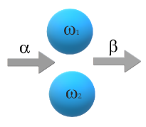
Figure 1: Schematic setup showing two single-occupancy quantum dots with external biases (denoted with arrows) corresponding to the non-number-conserving interactions with coefficients $\alpha$ and $\beta$.

For the fermionic system at hand, the complete Hilbert space can be decomposed as

$$\mathcal{H}=\mathcal{H}_{0}\oplus\mathcal{H}_{1}\oplus\mathcal{H}_{2},$$ (4)

where $\mathcal{H}_{0}$ and $\mathcal{H}_{2}$ are one-dimensional (each) and are spanned by the vectors $|\Omega\rangle$ and $c_{1}^{\dagger}c_{2}^{\dagger}|\Omega\rangle$, respectively; $\mathcal{H}_{1}$ is two-dimensional and is spanned by $c_{1}^{\dagger}|\Omega\rangle$ and $c_{2}^{\dagger}|\Omega\rangle$. Here $|\Omega\rangle$ is the zero-particle (vacuum) state. We relabel the basis vectors as $|1\rangle:=|\Omega\rangle$, $|2\rangle:=c_{1}^{\dagger}|\Omega\rangle$, $|3\rangle:=c_{2}^{\dagger}|\Omega\rangle$, and $|4\rangle:=c_{1}^{\dagger}c_{2}^{\dagger}|\Omega\rangle$. In this (natural) basis, the Hamiltonian is expressible as a $4\times 4$ matrix which reads

$$H=\begin{pmatrix}0&0&0&\beta\\ 0&\omega_{1}&0&0\\ 0&0&\omega_{2}&0\\ \alpha&0&0&(\omega_{1}+\omega_{2})\\ \end{pmatrix}.$$ (5)

It should be remarked that just as the (bosonic) Swanson oscillator, the fermionic extension is pseudo-hermitian, i.e., one can find some matrix $\eta$, such that $h=\eta^{-1}H\eta$ is hermitian. For instance, picking $\omega_{1}=\omega$ and $\omega_{2}=1-\omega$, with $\omega\in(0,1)$, we have

$$\eta=\begin{pmatrix}-\frac{1+\sqrt{1+4\alpha\beta}}{2\beta}&-\frac{1-\sqrt{1+4\alpha\beta}}{2\beta}&0&0\\ 0&0&0&1\\ 0&0&1&0\\ 1&1&0&0\\ \end{pmatrix},$$ (6)

giving

$$h=\begin{pmatrix}\frac{1}{2}(1-\sqrt{1+4\alpha\beta})&0&0&0\\ 0&\frac{1}{2}(1+\sqrt{1+4\alpha\beta})&0&0\\ 0&0&(1-\omega)&0\\ 0&0&0&\omega\\ \end{pmatrix},$$ (7)

which is hermitian. In what follows, we explore the existence of exceptional points associated with $H$.

III Eigenstates, parameter space, and exceptional points

For ease of demonstration, we go for the choice $\omega_{1}=\omega$ and $\omega_{2}=1-\omega$, with $\omega\in(0,1)$. The four-dimensional problem admits four eigenstates. Two of the right eigenvectors in the $\{|1\rangle,|2\rangle,|3\rangle,|4\rangle\}$ basis are

$$|\psi^{\rm I}_{R}\rangle=\begin{pmatrix}-\frac{\sqrt{4\alpha\beta+1}+1}{2\alpha}\\ 0\\ 0\\ 1\\ \end{pmatrix},\hskip 14.22636pt|\psi^{\rm II}_{R}\rangle=\begin{pmatrix}-\frac{1-\sqrt{4\alpha\beta+1}}{2\alpha}\\ 0\\ 0\\ 1\\ \end{pmatrix},$$ (8)

with respective eigenvalues $E^{\rm I,II}=\frac{1}{2}\left(1\mp\sqrt{4\alpha\beta+1}\right)$. The other two eigenvectors are

$$|\psi^{\rm III}_{R}\rangle=\begin{pmatrix}0\\ 1\\ 0\\ 0\\ \end{pmatrix},\hskip 14.22636pt|\psi^{\rm IV}_{R}\rangle=\begin{pmatrix}0\\ 0\\ 1\\ 0\\ \end{pmatrix},$$ (9)

with respective eigenvalues $E^{\rm III,IV}=\omega,1-\omega$.

III.1 Exceptional points

The states described by $|\psi^{\rm III,IV}_{R}\rangle$ are independent of the ‘non-Hermiticity’ parameters $\alpha$ and $\beta$, and therefore cannot be made to coalesce by tuning the parameters $\alpha$ and $\beta$. On the other hand, it is clear that the states described by $|\psi^{\rm I,II}_{R}\rangle$ depend upon $\alpha$ and $\beta$ rather strongly. The corresponding left eigenvectors read

$$\langle\psi^{\rm I}_{L}|=\begin{pmatrix}-\frac{\sqrt{4\alpha\beta+1}+1}{2\beta}\\ 0\\ 0\\ 1\\ \end{pmatrix}^{T},\hskip 14.22636pt\langle\psi^{\rm II}_{L}|=\begin{pmatrix}-\frac{1-\sqrt{4\alpha\beta+1}}{2\beta}\\ 0\\ 0\\ 1\\ \end{pmatrix}^{T}.$$ (10)

At an exceptional point, it is expected that both the eigenvalues and the eigenvectors coalesce. For the present case, it is found to happen for $1+4\alpha\beta=0$, for which $E^{\rm I}=E^{\rm II}=\frac{1}{2}$ and $|\psi^{\rm I}_{R}\rangle=|\psi^{\rm II}_{R}\rangle$; quite naturally then, one also has $\langle\psi^{\rm I}_{L}|=\langle\psi^{\rm II}_{L}|$, which gives

$$\langle\psi^{\rm I,II}_{L}|\psi^{\rm I,II}_{R}\rangle=\frac{1}{4\alpha\beta}+1=0,$$ (11)

confirming the self-orthogonality condition EP . In Fig. (2), we have plotted the eigenvalues $E^{\rm I,II}$ as a function of $\alpha$ and $\beta$. On the $\alpha\beta$-parameter space, the rectangular hyperbola $4\alpha\beta+1=0$ describes the set of points (infinitely many) for which the eigenvalues and eigenvectors coalesce. Thus, the condition $4\alpha\beta+1=0$ may be interpreted as pointing to the ‘exceptional curve’.

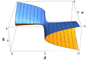
Figure 2: 3D plot of $E^{\rm I,II}$ (labelled as $E$) as a function of $\alpha$ and $\beta$ for $\alpha,\beta\in\mathbb{R}$. The two eigenvalues are indicated by the two different colors.

III.2 $\alpha\beta$-parameter space

Let us comment on the parameter space which is induced by the parameters $\alpha$ and $\beta$ (assuming $\alpha,\beta\neq 0$). Since we are looking for real eigenvalues, we restrict our attention to the points for which $4\alpha\beta+1\geq 0$. We note that the norm of the states ‘I’ and ‘II’ can be determined to be

$$\langle\psi^{\rm I}_{L}|\psi^{\rm I}_{R}\rangle=1+\frac{(1+\sqrt{4\alpha\beta+1})^{2}}{4\alpha\beta},$$ (12)

$$\langle\psi^{\rm II}_{L}|\psi^{\rm II}_{R}\rangle=1+\frac{(1-\sqrt{4\alpha\beta+1})^{2}}{4\alpha\beta}.$$ (13)

Although the norms coalesce and vanish at exceptional points for which $4\alpha\beta+1=0$, demanding that they are to be positive furnishes the additional condition $\alpha\beta>0$. In Fig. (3), the region shaded in dark gray (the first and third quadrants excluding the lines $\alpha=0$ and $\beta=0$) are where the following two conditions hold: (a) spectrum is real, (b) norms are positive. The region shaded in light gray contains those points for which the norms $\langle\psi^{\rm I}_{L}|\psi^{\rm I}_{R}\rangle$ and $\langle\psi^{\rm II}_{L}|\psi^{\rm II}_{R}\rangle$ are not positive definite (they are rather complex valued in general), although the spectrum is still real. The exceptional curve $4\alpha\beta+1=0$ is shown as a dashed curve, at which the norms coalesce to zero.

Figure 3: Region in the $\alpha\beta$-parameter space conforming to $4\alpha\beta+1>0$ (light and dark gray) and $\alpha\beta>0$ (dark gray). The black-dashed curve is $4\alpha\beta+1=0$.

IV Ground-State Entanglement Spectrum and Entanglement Entropy

Let us evaluate the entanglement spectrum of the ground state by performing a partial trace over one of the fermions. We adopt two distinct ways to approach the problem; the first one is based on the bi-orthogonal interpretation of non-hermitian quantum mechanics biortho , while the second one uses a Dirac-normalization scheme (see for instance, ref. dirac ) to produce right and left (reduced) density matrices rhoref1 . Below, we briefly digress upon the two above-mentioned schemes.

In the bi-orthogonal scheme, for a generic eigenstate with right and left eigenvectors $|\psi_{R}\rangle$ and $\langle\psi_{L}|$, respectively, one forms the norm as $||\psi||=\sqrt{\langle\psi_{L}|\psi_{R}\rangle}$, while the expectation value of some operator $\mathcal{O}$ reads as $\langle\psi_{L}|\mathcal{O}|\psi_{R}\rangle$. The states can be bi-normalized by redefining $|\psi^{N}_{R}\rangle\rightarrow\frac{|\psi^{N}_{R}\rangle}{\sqrt{\langle\psi_{L}|\psi_{R}\rangle}}$ and $\langle\psi^{N}_{L}|\rightarrow\frac{\langle\psi^{N}_{L}|}{\sqrt{\langle\psi_{L}|\psi_{R}\rangle}}$, such that $\langle\psi^{N}_{L}|\psi^{N}_{R}\rangle=1$. This produces reliable results, especially for the reduced density matrix that is described subsequently, provided that $\langle\psi_{L}|\psi_{R}\rangle>0$ for non-trivial eigenvectors. This however, cannot be guaranteed in general; for instance, the norms given in Eqs. (12) and (13) are positive definite only for parameter choices satisfying $\alpha\beta>0$. For the other cases where the norms are not positive definite, one can resort to the so-called Dirac norms $\langle\psi_{L}|\psi_{L}\rangle$ and $\langle\psi_{R}|\psi_{R}\rangle$, which are guaranteed to be positive definite for non-trivial eigenvectors. One then has either left or right normalization, which can produce positive-semidefinite (reduced) density matrices. In what follows, we compute the ground-state entanglement spectrum and entanglement entropy via the two schemes briefly discussed above.

IV.1 Density matrix from bi-normalization

We consider the situation where Eqs. (12) and (13) describe positive-definite norms, i.e., we consider parameter values from the region shaded in dark gray in Fig. (3). It is equivalent to the condition $\alpha\beta>0$, for which in the $\{|1\rangle,|2\rangle,|3\rangle,|4\rangle\}$ basis, the ground state is described by

$$|G_{R}\rangle=\begin{pmatrix}-\frac{\sqrt{4\alpha\beta+1}+1}{2\alpha}\\ 0\\ 0\\ 1\\ \end{pmatrix},\hskip 14.22636pt\langle G_{L}|=\begin{pmatrix}-\frac{\sqrt{4\alpha\beta+1}+1}{2\beta}\\ 0\\ 0\\ 1\\ \end{pmatrix}^{T}.$$ (14)

For constructing the (reduced) density matrix, we bi-normalize them as

$$|G^{N}_{R}\rangle:=\frac{|G_{R}\rangle}{\sqrt{\langle G_{L}|G_{R}\rangle}},\hskip 14.22636pt\langle G^{N}_{L}|:=\frac{\langle G_{L}|}{\sqrt{\langle G_{L}|G_{R}\rangle}},$$ (15)

where $\langle G_{L}|G_{R}\rangle=1+\frac{(1+\sqrt{4\alpha\beta+1})^{2}}{4\alpha\beta}$. The strategy towards finding the reduced density matrix for one of the fermions, say fermion ‘1’ is as follows (see ent for some related discussions). The algebra of the observables corresponding to the first oscillator is essentially generated by $\{\mathbb{I},c_{1},c_{1}^{\dagger}\}$ and thus, the reduced density matrix could be expressible in the manner

$$\rho_{1}=a_{0}\mathbb{I}+a_{1}c_{1}+a_{2}c_{1}^{\dagger}+a_{3}c_{1}^{\dagger}c_{1},$$ (16)

for some coefficients $\{a_{0},a_{1},a_{2},a_{3}\}$. Now, for a generic observable $\mathcal{O}$ from this algebra, one has the following equality

$${\rm Tr}_{1}[\rho_{1}\mathcal{O}]=\langle G_{L}^{N}|\mathcal{O}|G_{R}^{N}\rangle,$$ (17)

where ${\rm Tr}_{1}[\cdot]$ is evaluated on the basis $|\Omega\rangle$ and $c_{1}^{\dagger}|\Omega\rangle$. This serves as a consistency condition allowing one to determine the constants $\{a_{0},a_{1},a_{2},a_{3}\}$. A straightforward computation leads to

$$\rho_{1}=\begin{pmatrix}\frac{\mu_{1}\mu_{2}}{1+\mu_{1}\mu_{2}}&0\\ 0&\frac{1}{1+\mu_{1}\mu_{2}}\end{pmatrix},$$ (18)

where $\mu_{1}=\frac{\sqrt{4\alpha\beta+1}+1}{2\alpha}$ and $\mu_{2}=\frac{\sqrt{4\alpha\beta+1}+1}{2\beta}$. Notice that ${\rm Tr}_{1}[\rho]=1$, as anticipated. Moreover, for consistency, one requires $\mu_{1}\mu_{2}\geq 0$, which is equivalent to the restriction $\alpha\beta>0$. In Fig. (4), we have plotted the ground-state entanglement spectrum, i.e., the elements $(\rho_{1})_{11}$ and $(\rho_{1})_{22}$ as functions of $\alpha\beta$, from which one clearly sees that $(\rho_{1})_{22}$ becomes negative for $\alpha\beta<0$, although one still has $(\rho_{1})_{11}+(\rho_{1})_{22}=1$. We may now easily compute the ground-state entanglement entropy from the standard representation

$$S(\rho_{1})=-{\rm Tr}_{1}[\rho_{1}\ln\rho_{1}],$$ (19)

which is plotted in Fig. (5) as a function of $\alpha\beta$. It is found that it is nearly zero for $\alpha\beta\approx 0$ and increases as $\alpha\beta$ is increased, approaching finally towards $\ln 2$, which is the maximum entropy of a two-state system.

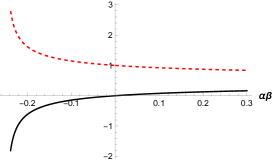
Figure 4: Ground-state entanglement spectrum, $(\rho_{1})_{11}$ (red) and $(\rho_{1})_{22}$ (black) as a function of $\alpha\beta$, justifying the choice of parameters for which $\alpha\beta>0$.

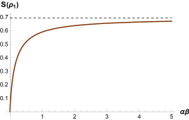
Figure 5: Ground-state entanglement entropy as a function of $\alpha\beta$. The dashed line corresponds to $\ln 2$.

IV.2 Right density matrix

Notice that in the preceding discussion, we considered $\alpha\beta>0$, thereby excluding parameters from the region shaded in light gray in Fig. (3), for which the spectrum is real but Eqs. (12) and (13) are complex-valued norms that coalesce to zero for $4\alpha\beta+1=0$. Thus, we can no longer rely on the bi-normalization procedure as given in Eq. (15) to produce a reduced density matrix that is positive semidefinite. Instead, we may normalize using the Dirac norms dirac $\langle G_{R}|G_{R}\rangle$ and $\langle G_{L}|G_{L}\rangle$, which lead to right and left (reduced) density matrices, respectively (see rhoref1 and references therein). Below, we focus on the right density matrix.

Let us analyze the special case for which $\omega\leq\frac{1}{2}$, and then ground-state energy reads

$$E_{G} = \omega,\hskip 91.04881pt-\frac{1}{4}<\alpha\beta<\omega^{2}-\omega,$$ (20)

$$= \frac{1}{2}\left(1-\sqrt{4\alpha\beta+1}\right),\hskip 14.22636pt\alpha\beta>\omega^{2}-\omega.$$

For the purpose of illustration, we have plotted all the four eigenvalues as a function of $\alpha\beta$ in Fig. (6) for the choice $\omega=1/4$, and one can observe a ground-state crossing. The ground state reads as

$$|G_{R}\rangle=\begin{pmatrix}0\\ 1\\ 0\\ 0\\ \end{pmatrix},$$ (21)

for $-\frac{1}{4}<\alpha\beta<\omega^{2}-\omega$, and

$$|G_{R}\rangle=\begin{pmatrix}-\frac{\sqrt{4\alpha\beta+1}+1}{2\alpha}\\ 0\\ 0\\ 1\\ \end{pmatrix},$$ (22)

for $\alpha\beta>\omega^{2}-\omega$. We denote the corresponding reduced density matrix for the fermion ‘1’ as $\rho_{1}$, such that

$${\rm Tr}_{1}[\rho_{1}\mathcal{O}]=\frac{\langle G_{R}|\mathcal{O}|G_{R}\rangle}{\langle G_{R}|G_{R}\rangle}.$$ (23)

It then simply follows that

$$\rho_{1}=\begin{pmatrix}0&0\\ 0&1\\ \end{pmatrix},$$ (24)

for $-\frac{1}{4}<\alpha\beta<\omega^{2}-\omega$, while

$$\rho_{1}=\begin{pmatrix}\lambda_{11}&0\\ 0&\lambda_{22}\\ \end{pmatrix},$$ (25)

for $\alpha\beta>\omega^{2}-\omega$. Here, $\lambda_{22}=\big{[}1+\left(\frac{1+\sqrt{1+4z_{2}}}{2z_{1}}\right)^{2}\big{]}^{-1}$ and $\lambda_{11}=1-\lambda_{22}$, with $\alpha=z_{1},\beta=\frac{z_{2}}{z_{1}}$; for $\alpha\neq 0$ the transformation $(\alpha,\beta)\rightarrow(z_{1},z_{2})$ is well defined and is invertible. We have plotted the ground-state entanglement entropy in Fig. (7) which shows a discontinuous jump between the two regimes $-\frac{1}{4}<\alpha\beta<\omega^{2}-\omega$ and $\alpha\beta>\omega^{2}-\omega$. This seems to indicate a quantum phase transition, being characterized by the discontinuous jump in the entanglement entropy due to the ground-state crossing sachdev .

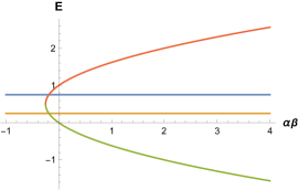
Figure 6: Energy eigenvalues $E^{\rm I}$ (green), $E^{\rm II}$ (orange), $E^{\rm III}$ (yellow), and $E^{\rm IV}$ (blue), as a function of $\alpha\beta$. We have chosen $\omega=1/4$.

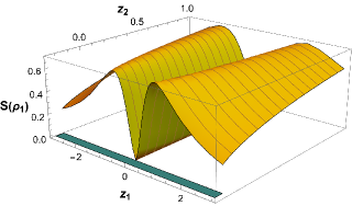
Figure 7: Ground-state entanglement entropy as a function of $z_{1}$ and $z_{2}$. The discontinuity between the yellow and blue-green regions indicates the phase transition.

It should be emphasized that we have normalized the ground state here with respect to the ‘right’ Dirac norm $\langle G_{R}|G_{R}\rangle$, such that the reduced density matrix so obtained turns out to be positive semidefinite. One could have alternatively employed the ‘left’ Dirac norm $\langle G_{L}|G_{L}\rangle$ and then, the result for the reduced density matrix and entanglement entropy would have the same form as obtained above under the interchange $\alpha\leftrightarrow\beta$. The same phase transition can be observed for both the cases, and since the ground-state crossing happens for parameter values for which $\alpha\beta<0$, no such phase transition was observed in Sec. (IV.1), in which we specifically restricted ourselves to the cases with $\alpha\beta>0$.

V Concluding Remarks

We have proposed a fermionic extension of the Swanson oscillator, which admits a quadratic but non-hermitian Hamiltonian by including terms which do not conserve particle number. We have shown that our proposed model admits of an infinite number of exceptional points, being given by the points residing on the exceptional curve $4\alpha\beta+1=0$. Restricting to parameter values which produce a positive norm (in the sense of bi-normalization of left and right eigenvectors) and a real spectrum, we have computed the entanglement spectrum and entanglement entropy of the ground state in Sec. (IV.1). In Sec. (IV.2), upon adopting a different scheme which relies on Dirac normalization rather than bi-normalization, we were able to compute the entanglement spectrum even in the region of the parameter space for which the norms given in Eqs. (12) and (13) turn out to be complex, coalescing to zero at the exceptional points. A quantum phase transition was observed, which corresponds to the ground-state crossing. The analogous number-preserving case is presented in Appendix (A).

It is now well-understood that non-hermitian Hamiltonians describe open quantum systems, and that an effective non-hermitian description can be heuristically obtained starting from a system + environment approach, by obtaining a quantum master equation for the reduced density operator of the ‘open’ system and then disregarding the so-called jump operators (see for instance, ref. NH4 ). Thus, it would be quite interesting to explore the kind of system + environment (hermitian) description which would lead to Swanson-like Hamiltonians in describing the system’s reduced density operator. We keep this issue for future work.

Acknowledgements: We thank Jasleen Kaur for carefully reading the manuscript and for help in preparing the schematic figures. A.S. thanks P. Padhmanabhan and A. P. Balachandran for useful discussions, and also acknowledges the financial support from IIT Bhubaneswar in the form of an Institute Research Fellowship. A.G. is thankful to Manas Kulkarni for some discussions. The work of A.G. is supported by Ministry of Education (MoE), Government of India in the form of a Prime Minister’s Research Fellowship (ID: 1200454). B.B. thanks Brainware University for infrastructural support.

Appendix A Two-fermion model with non-hermitian and number-conserving interactions

In this appendix, we consider the situation with bilinear-coupling terms between the two fermions that conserve particle number, i.e., we have terms that go as $c_{1}^{\dagger}c_{2}$ and $c_{2}^{\dagger}c_{1}$. Then, the Hamiltonian has the form

$$H=\omega_{1}c_{1}^{\dagger}c_{1}+\omega_{2}c_{2}^{\dagger}c_{2}+\gamma c_{1}^{\dagger}c_{2}+\delta c_{2}^{\dagger}c_{1},$$ (26)

where $\omega_{1,2},\gamma,\delta\in\mathbb{R}$, with $\omega_{1,2}>0$ and $\gamma\neq\delta$. A schematic diagram is shown in Fig. (8).

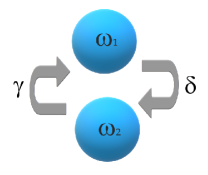
Figure 8: Schematic setup showing two single-occupancy quantum dots with number-conserving interactions (denoted with arrows) characterized by the coefficients $\gamma$ and $\delta$.

As before, the Hilbert space is four-dimensional and may be decomposed as $\mathcal{H}=\mathcal{H}_{0}\oplus\mathcal{H}_{1}\oplus\mathcal{H}_{2}$. In terms of the basis vectors $|1\rangle:=|\Omega\rangle$, $|2\rangle:=c_{1}^{\dagger}|\Omega\rangle$, $|3\rangle:=c_{2}^{\dagger}|\Omega\rangle$, and $|4\rangle:=c_{1}^{\dagger}c_{2}^{\dagger}|\Omega\rangle$, $H$ has the following matrix representation:

$$H=\begin{pmatrix}0&0&0&0\\ 0&\omega_{1}&\gamma&0\\ 0&\delta&\omega_{2}&0\\ 0&0&0&(\omega_{1}+\omega_{2})\\ \end{pmatrix}.$$ (27)

Resorting to the choice $\omega_{1}=\omega$ and $\omega_{2}=1-\omega$, for $\omega\in(0,1)$, two of the right eigenvectors read

$$|\psi^{\rm I}_{R}\rangle=\begin{pmatrix}1\\ 0\\ 0\\ 0\\ \end{pmatrix},\hskip 14.22636pt|\psi^{\rm II}_{R}\rangle=\begin{pmatrix}0\\ 0\\ 0\\ 1\\ \end{pmatrix},$$ (28)

with eigenvalues $E^{\rm I,II}=0,1$. The remaining two right eigenvectors are

$$|\psi^{\rm III}_{R}\rangle=\begin{pmatrix}0\\ -\frac{\sqrt{4\gamma\delta+4\omega^{2}-4\omega+1}-2\omega+1}{2\delta}\\ 1\\ 0\\ \end{pmatrix},$$ (29)

$$|\psi^{\rm IV}_{R}\rangle=\begin{pmatrix}0\\ -\frac{-\sqrt{4\gamma\delta+4\omega^{2}-4\omega+1}-2\omega+1}{2\delta}\\ 1\\ 0\\ \end{pmatrix},$$ (30)

with the corresponding eigenvalues $E^{\rm III,IV}=\frac{1}{2}\left(1\mp\sqrt{4\gamma\delta+4\omega^{2}-4\omega+1}\right)$. The reality of the eigenvalues requires $4\gamma\delta+4\omega^{2}-4\omega+1\geq 0$, a condition that is dependent on the choice of $\omega$, unlike in the previously-studied case.

A.1 Exceptional points

Notice that the eigenvectors $|\psi^{\rm I,II}_{R}\rangle$ are insensitive to the choice of the parameters $\gamma$ and $\delta$, and therefore are not involved in coalescence at any point by tuning $\gamma$ and $\delta$. However, the eigenvectors $|\psi^{\rm III,IV}_{R}\rangle$ and the corresponding eigenvalues $E^{\rm III,IV}$ may coalesce for particular values of $\gamma$ and $\delta$. Such a coalescence occurs for points on the rectangular hyperbola $4\gamma\delta+4\omega^{2}-4\omega+1=0$, on the $\gamma\delta$-parameter space (fixing $\omega$). In a sense, therefore, one has an exceptional curve (rather than isolated points) in the parameter space. The left eigenvectors $\langle\psi^{\rm III,IV}_{L}|$ are computed straightforwardly as

$$\langle\psi^{\rm III}_{L}|=\begin{pmatrix}0\\ -\frac{\sqrt{4\gamma\delta+4\omega^{2}-4\omega+1}-2\omega+1}{2\gamma}\\ 1\\ 0\\ \end{pmatrix}^{T},$$ (31)

$$\langle\psi^{\rm IV}_{L}|=\begin{pmatrix}0\\ -\frac{-\sqrt{4\gamma\delta+4\omega^{2}-4\omega+1}-2\omega+1}{2\gamma}\\ 1\\ 0\\ \end{pmatrix}^{T}.$$ (32)

At exceptional points, i.e., for $4\gamma\delta+4\omega^{2}-4\omega+1=0$, one finds that $|\psi^{\rm III}_{R}\rangle=|\psi^{\rm IV}_{R}\rangle$ (and also $\langle\psi^{\rm III}_{L}|=\langle\psi^{\rm IV}_{L}|$), along with $E^{\rm III}=E^{\rm IV}=1/2$. Thus, it is straightforward to verify that $\langle\psi^{\rm III,IV}_{L}|\psi^{\rm III,IV}_{R}\rangle=0$, reproducing the self-orthogonality relation.

A.2 Ground-state entanglement

Let us now describe entanglement properties of the ground state in this model. Some intriguing features can be exposed, for which we pick $\omega=1/2$. In this case, we must restrict ourselves to parameter choices leading to $\gamma\delta>0$ to ensure that the spectrum is real. The eigenvalues corresponding to the four eigenstates are plotted in Fig. (9) and for $\gamma\delta=1/4$, one observes a ground-state crossing.

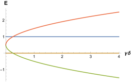
Figure 9: Energy eigenvalues $E^{\rm I}$ (yellow), $E^{\rm II}$ (blue), $E^{\rm III}$ (green), and $E^{\rm IV}$ (orange), as a function of $\gamma\delta$. We have chosen $\omega=1/2$.

Thus, $|\psi^{\rm I}\rangle$ describes the ground state for $\gamma\delta<1/4$, while $|\psi^{\rm III}\rangle$ describes the ground state for $\gamma\delta>1/4$. The corresponding reduced density matrix for the fermion ‘1’ can be obtained by the procedure described in the previous section. It reads

$$\rho_{1}=\begin{pmatrix}1&&0\\ 0&&0\\ \end{pmatrix},\hskip 14.22636pt\gamma\delta<\frac{1}{4},$$ (33)

and

$$\rho_{1}=\begin{pmatrix}\frac{1}{2}&&0\\ 0&&\frac{1}{2}\\ \end{pmatrix},\hskip 14.22636pt\gamma\delta>\frac{1}{4}.$$ (34)

The entanglement entropy, i.e., $S(\rho_{1})=-{\rm Tr}_{1}[\rho_{1}\ln\rho_{1}]$, is $0$ when $\gamma\delta<\frac{1}{4}$ and jumps to $\ln 2$ when $\gamma\delta>\frac{1}{4}$. This indicates a quantum phase transition, being characterized by the discontinuous jump in the entanglement entropy at $\gamma\delta=1/4$, as shown in Fig. (10).

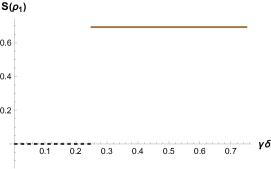
Figure 10: Entanglement entropy of the ground state showing a discontinuous jump at $\gamma\delta=1/4$, indicative of a phase transition.

It should be remarked that although we have picked $\omega=1/2$ to simplify our calculations, similar discontinuous jumps can be observed for other values of $\omega\in(0,1)$. One could similarly define reduced density matrices by considering the Dirac-normalization scheme as in Sec. (IV.2). In that case, one still observes the phase transition due to the ground-state crossing. We do not pursue this further as the calculations can be easily performed in the same spirit as those presented in Sec. (IV.2).

References

- (1) I. Rotter, A non-hermitian Hamilton operator and the physics of open quantum systems, J. Phys. A: Math. Theor. 42, 153001 (2009).
- (2) Y. Michishita and R. Peters, Equivalence of Effective Non-Hermitian Hamiltonians in the Context of Open Quantum Systems and Strongly Correlated Electron Systems, Phys. Rev. Lett. 124, 196401 (2020).
- (3) K. Holmes, W. Rehman, S. Malzard, and E.-M. Graefe, Husimi Dynamics Generated by non-Hermitian Hamiltonians, Phys. Rev. Lett. 130, 157202 (2023).
- (4) E.-M. Graefe, M. Höning, and H. J. Korsch, Classical limit of non-hermitian quantum dynamics – a generalized canonical structure, J. Phys. A: Math. Theor. 43, 075306 (2010).
- (5) Á. Gómez-León, T. Ramos, A. González-Tudela, and D. Porras, Bridging the gap between topological non-Hermitian physics and open quantum systems, Phys. Rev. A 106, L011501 (2022).
- (6) X. Niu, J. Li, S. L. Wu, and X. X. Yi, Effect of quantum jumps on non-Hermitian systems, Phys. Rev. A 108, 032214 (2023).
- (7) C. M. Bender and S. Boettcher, Real Spectra in Non-Hermitian Hamiltonians Having Symmetry, Phys. Rev. Lett. 80, 5243 (1998).
- (8) C. M. Bender, S. Boettcher, and P. N. Meisinger, -symmetric quantum mechanics, J. Math. Phys. 40, 2201 (1999).
- (9) C. M. Bender and D. W. Hook, -symmetric quantum mechanics, arXiv: 2312.17386 [quant-ph].
- (10) R. El-Ganainy, K. G. Makris, M. Khajavikhan, Z. H. Musslimani, S. Rotter, and D. N. Christodoulides, Non-Hermitian physics and PT symmetry, Nat. Phys. 14, 11 (2018).
- (11) Z. H. Musslimani, K. G. Makris, R. El-Ganainy, and D. N. Christodoulides, Optical Solitons in Periodic Potentials, Phys. Rev. Lett. 100, 030402 (2008).
- (12) L. Feng, R. El-Ganainy, and L. Ge, Non-Hermitian photonics based on parity–time symmetry, Nat. Photonics 11, 752 (2017).
- (13) R. El-Ganainy, M. Khajavikhan, D. N. Christodoulides, and S. K. Ozdemir, The dawn of non-Hermitian optics, Commun. Phys. 2, 37 (2019).
- (14) C. Wang, Z. Fu, W. Mao, J. Qie, A. D. Stone, and L. Yang, Non-Hermitian optics and photonics: from classical to quantum, Adv. Opt. Photonics 15, 442 (2023).
- (15) W. D. Heiss, The physics of exceptional points, J. Phys. A: Math. Theor. 45, 444016 (2012).
- (16) M. Znojil, Exceptional points and domains of unitarity for a class of strongly non-Hermitian real-matrix Hamiltonians, J. Math. Phys. 62, 052103 (2021).
- (17) T. Kato, Perturbation Theory for Linear Operators: Classics in Mathematics, Springer (1995).
- (18) F. Correa and M. L. Plyushchay, Spectral singularities in symmetric periodic finite-gap systems, Phys. Rev. D 86, 085028 (2012).
- (19) K. Zelaya and O. Rosas-Ortiz, Exact Solutions for Time-Dependent Non-Hermitian Oscillators: Classical and Quantum Pictures, Quantum Rep. 3, 458 (2021).
- (20) V. Fernández, R. Ramírez, and M. Reboiro, Swanson Hamiltonian: non-PT-symmetry phase, J. Phys. A: Math. Theor. 55, 015303 (2022).
- (21) I. Mandal and E. J. Bergholtz, Symmetry and Higher-Order Exceptional Points, Phys. Rev. Lett. 127, 186601 (2021).
- (22) M.-A. Miri and A. Alú, Exceptional points in optics and photonics, Science 363, eaar7709 (2019).
- (23) J. Wiersig, Review of exceptional point-based sensors, Photonics Res. 8, 1457 (2020).
- (24) A. Li, H. Wei, M. Cotrufo, W. Chen, S. Mann, X. Ni, B. Xu, J. Chen, J. Wang, S. Fan, C.-W. Qiu, A. Alú, and L. Chen, Exceptional points and non-hermitian photonics at the nanoscale, Nat. Nanotechnol. 18, 706 (2023).
- (25) C. Liang, Y. Tang, A.-N. Xu, and Y.-C. Liu, Observation of Exceptional Points in Thermal Atomic Ensembles, Phys. Rev. Lett. 130, 263601 (2023).
- (26) T. Goldzak, A. A. Mailybaev, and N. Moiseyev, Light Stops at Exceptional Points, Phys. Rev. Lett. 120, 013901 (2018).
- (27) M. S. Swanson, Transition elements for a non-hermitian quadratic Hamiltonian, J. Math. Phys. 45, 585 (2004).
- (28) E.-M. Graefe, H. J. Korsch, A. Rush, and R. Schubert, Classical and quantum dynamics in the (non-hermitian) Swanson oscillator, J. Phys. A: Math. Theor. 48, 055301 (2015).
- (29) B. Bagchi and I. Marquette, New 1-step extension of the Swanson oscillator and superintegrability of its two-dimensional generalization, Phys. Lett. A 379, 1584 (2015).
- (30) A. Fring and M. H. Y. Moussa, Non-Hermitian Swanson model with a time-dependent metric, Phys. Rev. A 94, 042128 (2016).
- (31) H. F. Jones, On pseudo-Hermitian Hamiltonians and their Hermitian counterparts, J. Phys. A: Math. Gen. 38, 1741 (2005).
- (32) B. Bagchi, R. Ghosh, and S. Sen, Exceptional point in a coupled Swanson system, EPL 137, 50004 (2022).
- (33) D. C. Brody, Biorthogonal quantum mechanics, J. Phys. A: Math. Theor. 47, 035305 (2014).
- (34) F. Ruzicka, K. S. Agarwal, and Y. N. Joglekar, Conserved quantities, exceptional points, and antilinear symmetries in non-hermitian systems, J. Phys.: Conf. Ser. 2038, 012021 (2021).
- (35) L. Herviou, N. Regnault, and J. H. Bardarson, Entanglement spectrum and symmetries in non-Hermitian fermionic non-interacting models, SciPost Phys. 7, 069 (2019).
- (36) A. F. Reyes-Lega, Some aspects of operator algebras in quantum physics, Geometric, Algebraic, and Topological Methods for Quantum Field Theory: Proceedings of the 2013 Villa de Leyva Summer School, Villa de Leyva, Colombia, 15–27 July 2013, pp. 1-74 (2017).
- (37) S. Sachdev, Quantum Phase Transitions, 2nd. ed., Cambridge University Press (2011).