Detailed Error Analysis of the HHL Algorithm

Abstract

We reiterate the contribution made by Harrow, Hassidim, and Llyod to the quantum matrix equation solver with the emphasis on the algorithm description and the error analysis derivation details. Moreover, the behavior of the amplitudes of the phase register on the completion of the Quantum Phase Estimation is studied. This study is beneficial for the comprehension of the choice of the phase register size and its interrelation with the Hamiltonian simulation duration in the algorithm setup phase.

Keywords HHL algorithm  $\cdot$ Error Analysis

1 Introduction

The seminal paper Harrow et al. (2009) proposes the quantum matrix equation solver, commonly referred to as the HHL algorithm. Compared to classical matrix equation solvers, the HHL algorithm offers exponential speedup thanks to the expressive power of quantum information storage and processing. For a matrix equation $A\mathbf{x}=\mathbf{b}$, the HHL algorithm seeks to prepare a quantum state $\ket{x}$ that is proportional to the desired solution vector $\bm{x}$. When the matrix $A$ is $s$-sparse, i.e., containing at most $s$ nonzero elements per row/column, the HHL algorithm completes in $\tilde{O}(\log(N)s^{2}\kappa^{2}/\epsilon)$ with a target error level $\epsilon$, where $\kappa$ is the condition number of $A$. A conjugate gradient method Shewchuk et al. (1994), would instead complete in ${O}(Ns\kappa\log(1/\epsilon))$ in general (when $A$ is not necessarily positive definite). Hence, the HHL algorithm achieves exponential speedup over $N$, even though containing a worse dependence on $s$, $\kappa$, and $\epsilon$. The quadratic dependence on $s$ is acceptable assuming $s$ being a small number, and in a dense matrix equation case, the HHL is extended in Wossnig et al. (2018). The worse dependence on the condition number and error is addressed by Clader et al. (2013) and Childs et al. (2017)

Note that the outcome of the HHL algorithm is a quantum state, so subsequent quantum post-processing is assumed, otherwise the exponential speedup is voided if the entire vector needs to be transformed into a classical memory (writing down the solution would take $O(N)$ time). One circumstance and important application in which the HHL speedup is preserved is when the expectation with respect to some observable $M$, i.e., $\mathbf{x}^{\dagger}M\mathbf{x}$ is of interest. In this case, such implementation of the observable as a quantum circuit at the end of the HHL circuit, and the expectation is obtained by measuring in an appropriate basis, a standard treatment in quantum algorithms Nielsen and Chuang (2010).

As the matrix equation is a basic linear algebraic procedure, it is no surprise that the HHL algorithm underpins a collection of other quantum algorithms Grant et al. (2018); Butler et al. (2018); Biamonte et al. (2017), which again underscores the pivotal role of understanding the HHL algorithm for a quantum software engineer. We note, however, that the HHL algorithm is not a near-term algorithm suitable for Noisy Intermediate-Scale Quantum (NISQ) devices Preskill (2018). Though research on near-term version of it has emerged Yalovetzky et al. (2021), the study of the HHL algorithm mainly remains theoretical level.

Despite being well-presented in the original paper overall, in this work, the theoretical framework of the HHL algorithm is revisited with added elaborations to derivation and proof, and corrections on typos/mistakes. The target of this work is to help readers understand the HHL algorithm in detail so that possible improvement can be instilled on this groundwork. We confine our scope to the study of the original HHL algorithm regardless of previously mentioned improvements Wossnig et al. (2018); Clader et al. (2013); Childs et al. (2017).

The paper is structured as follows. Section 2 covers the detailed breakdown of the HHL algorithm with recorded intermediate results of each step. Next, the behavior of the amplitudes of the phase register is studied in Section 3. This behavior is paramount in understanding the choice of the register size, as well as the study of the error. In Section 4, a detailed error analysis of the HHL algorithm is given with proofs and derivations.

2 Algorithm Details

Herein, we make the following assumptions for the matrix equation for simplicity:

• $A\in\mathbb{C}^{N\times N}$ is Hermitian, where $N$ is a power of 2 such that $n\coloneqq\log_{2}(N)$ is an integer.

• The condition number $\kappa$ of $A$ is known or can be efficiently approximated, and $A$ is scaled so that all of its eigenvalues belong to the region $[1/\kappa,1]$.

• $\bm{b}$ is a normalized vector so that it can be encoded into a quantum state $\ket{b}$.

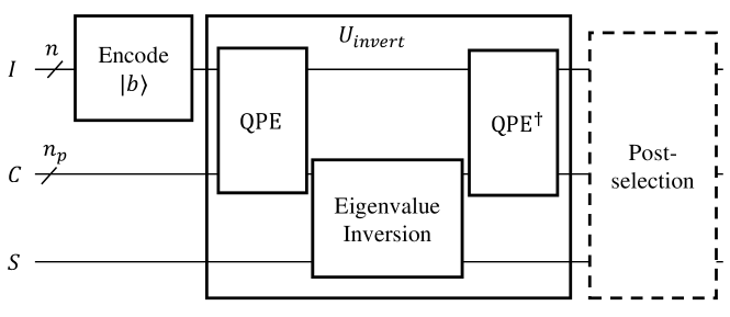
Figure 1: The diagram illustration of the HHL circuit.

The diagram of the HHL algorithm is given in Figure 1. The HHL circuit contains three registers: the Input/Output register $I$ with $n$ qubits; the Clock register $C$ with $n_{t}$ qubits; the Flag register $S$ that contains a qutrit (a quantum entity that lives in a 3-dimensional space). We define $T\coloneqq 2^{n_{t}}$ as the dimension of the Hilbert space encapsulating the statevectors in register $C$.

We assume that some other procedure Zhang et al. (2022) encodes state $\ket{b}$ into the register $I$, such that the initial state that $U_{invert}$ operates on is

$$\ket{\Phi_{0}}=\ket{b}_{I}\ket{0}_{C}\ket{\text{nothing}}_{S}=\sum_{j=0}^{N-1}\beta_{j}\ket{u_{j}}_{I}\ket{0}_{C}\ket{\text{nothing}}_{S},$$ (1)

where $\ket{b}$ is represented as $\sum_{j=0}^{N-1}\beta_{j}\ket{u_{j}}$ in the eigenbasis $\{\ket{u_{j}}\}$ of $A$: $A\ket{u_{j}}=\lambda_{j}\ket{u_{j}}$. The unitary operation $U_{invert}$ represents the HHL procedure that inverts the matrix $A$. It contains three components: quantum phase estimation (QPE), eigenvalue inversion, and the inverse of QPE.

The steps of a practical $U_{invert}$ are

1. QPE, denoted as a unitary operator $P$.

   1. Prepare the state $\ket{\Phi}=\sqrt{\frac{2}{T}}\sum_{\tau=0}^{T-1}\sin\left(\frac{\pi}{T}(\tau+\frac{1}{2})\right)\ket{\tau}$ on $C$. The state after this step is

      $$\ket{\Phi_{1}}=\sum_{j=0}^{N-1}\beta_{j}\ket{u_{j}}_{I}\sqrt{\frac{2}{T}}\sum_{\tau=0}^{T-1}\sin\left[\frac{\pi}{T}\left(\tau+\frac{1}{2}\right)\right]\ket{\tau}_{C}\ket{\text{nothing}}_{S}.$$ (2)

   2. Repeatedly apply the Hamiltonian simulation (HS) $e^{iAt_{0}/T}$ $\tau$ times to register $I$ conditioned on the state of the clock register $\ket{\tau}_{C}$, an operation represented as $\sum_{\tau=0}^{T-1}e^{iA(t_{0}/T)\tau}_{I}\otimes\ket{\tau}\bra{\tau}_{C}$. The choice of the HS time $t_{0}$ will be discussed in Section 3. The state of the circuit after the condition HS is

      $$\ket{\Phi_{2}}=\sum_{j=0}^{N-1}\beta_{j}\ket{u_{j}}_{I}\sqrt{\frac{2}{T}}\sum_{\tau=0}^{T-1}\sin\left[\frac{\pi}{T}\left(\tau+\frac{1}{2}\right)\right]e^{i\lambda_{j}(t_{0}/T)\tau}\ket{\tau}_{C}\ket{\text{nothing}}_{S}.$$ (3)

   3. Apply the quantum Fourier transform (QFT)

      $$\ket{\tau}_{C}\xrightarrow{\text{QFT}}\frac{1}{\sqrt{T}}\sum_{k=0}^{T-1}e^{-i(2\pi/T)k\tau}\ket{k}_{C}$$ (4)

      to register $C$. The resultant state is

      $$\ket{\Phi_{3}}=\sum_{j=0}^{N-1}\beta_{j}\ket{u_{j}}_{I}\sum_{k=0}^{T-1}\alpha_{k|j}\ket{k}_{C}\ket{\text{nothing}}_{S}$$ (5)

      where the amplitude is given as

      $$\alpha_{k|j}=\frac{\sqrt{2}}{T}\sum_{\tau=0}^{T-1}\sin\left[\frac{\pi}{T}\left(\tau+\frac{1}{2}\right)\right]e^{i\left(\lambda_{j}-\frac{2\pi}{t_{0}}k\right)\frac{t_{0}}{T}\tau}.$$ (6)

      The phase in (107) suggests the definition of the approximated eigenvalue (associated with state $\ket{k}_{C}$) as

      $$\tilde{\lambda}_{k}\coloneqq\frac{2\pi}{t_{0}}k.$$ (7)

      We further define $\delta_{\lambda}$ as the error in the eigenvalue approximation:

      $$\delta_{\lambda}(k|j)\coloneqq\lambda_{j}-\tilde{\lambda}_{k}.$$ (8)

   At this point we have covered all three steps of the QPE. The idea of QPE is that the magnitude of amplitude, $|\alpha_{k|j}|$, peaks when $\lvert\delta_{\lambda}\rvert$ is small, and decays when $\lvert\delta_{\lambda}\rvert$ is large, such that the terms with $k$ that yields a good eigenvalue approximation dominates. This behavior is essential to understanding the algorithm and the error analysis of the algorithm. We will elaborate on this in Section 3. Discreet reader might also notice that the lower and upper bounds of $k$ are not given in (5), we will give these in Section 3 as well.

2. Set the a flag register $S$ in the state

   $$\ket{h(\tilde{\lambda}_{k})}\coloneqq$$

   $$\quad\begin{cases}f(\tilde{\lambda}_{k})\ket{\text{well}}+g(\tilde{\lambda}_{k})\ket{\text{ill}}+\sqrt{1-f^{2}(\tilde{\lambda}_{k})-g^{2}(\tilde{\lambda}_{k})}\ket{\text{nothing}},&k=0,1,\cdots,K\\ \ket{\text{nothing}},&k=K+1,\cdots,T-1\end{cases}$$ (9)

   where the filter functions $f(\lambda)$ and $g(\lambda)$ are defined as

   $$f(\lambda)\coloneqq\begin{cases}\frac{1}{2\tilde{\kappa}\lambda},&\lambda\in\left[\frac{1}{\tilde{\kappa}},1\right]\\ -\frac{1}{2}\cos(\pi\tilde{\kappa}\lambda),&\lambda\in\left[\frac{1}{2\tilde{\kappa}},\frac{1}{\tilde{\kappa}}\right]\\ 0,&\lambda\in\left(0,\frac{1}{2\tilde{\kappa}}\right]\end{cases}$$ (10)

   $$g(\lambda)\coloneqq\begin{cases}0,&\lambda\in\left[\frac{1}{\tilde{\kappa}},1\right]\\ \frac{1}{2}\sin(\pi\tilde{\kappa}\lambda),&\lambda\in\left[\frac{1}{2\tilde{\kappa}},\frac{1}{\tilde{\kappa}}\right]\\ \frac{1}{2},&\lambda\in\left(0,\frac{1}{2\tilde{\kappa}}\right]\end{cases}$$ (11)

   where $\tilde{\kappa}$ is the approximation of the actual condition number $\kappa$ with the assumption that

   $$\tilde{\kappa}=O(\kappa).$$ (12)

   The cutoff value $K$ in (2) relates to the choice of $t_{0}$ and $T$, and will be discussed in the next section. The state after this step is

   $$\ket{\Phi_{4}}=\sum_{j=0}^{N-1}\beta_{j}\ket{u_{j}}_{I}\sum_{k=0}^{T-1}\alpha_{k|j}\ket{k}_{C}\ket{h(\tilde{\lambda}_{k})}_{S}.$$ (13)

3. Apply inverse QPE $P^{\dagger}$, i.e., apply the inverse of the three steps of QPE in reverse order to restore the $\ket{0}$ state in register $C$. The final state $\ket{\Phi_{f}}$ would be

   $$\ket{\Phi_{f}}=P^{\dagger}\sum_{j=0}^{N-1}\beta_{j}\ket{u_{j}}_{I}\sum_{k=0}^{T-1}\alpha_{k|j}\ket{k}_{C}\ket{h(\tilde{\lambda}_{k})}_{S}.$$ (14)

The final state (14) from the practical HHL circuit $QC_{practical}$ does not directly relate to the solution of the matrix equation $\bm{x}=\sum_{j=0}^{N-1}\frac{\beta_{j}}{\lambda_{j}}\ket{u_{j}}$ in an obvious way. This is because the non-ideal QPE, which does not guarantee that $|\alpha_{k|j}|=0$ when $|\delta_{\lambda}(k|j)|\neq 0$, results in the entanglement between the clock register $C$ and flag register $S$ in (13). This entanglement will still take place in the final state $\ket{\Phi_{f}}$, making its comparison with $\ket{x}$ hard.

To offer intuition on why HHL algorithm works, we consider an ideal HHL circuit $QC_{ideal}$, in which we suppose that the QPE reveals the exact eigenvalue. Let us use a overhead bar to distinguish the circuit components and quantum states of $QC_{ideal}$ from those of $QC_{practical}$. For example, $\bar{P}$ means the ideal QPE in $QC_{ideal}$. The final state of $QC_{ideal}$, $\ket{\bar{\Phi}_{f}}$ would be

$$\ket{\bar{\Phi}_{f}}=\sum_{j=0}^{N-1}\beta_{j}\ket{u_{j}}_{I}\ket{0}_{C}\ket{h(\lambda_{j})}_{S}.$$ (15)

The comparison between (15) and (2) indicates that if we post-select the final state depending on the state of the flag register $S$, we will retrieve a solution state $\ket{\bar{x}}$ that is proportional to the solution to the matrix equation $\bm{x}$, provided that all eigenvalues are in the well-conditioned region $[\frac{1}{\tilde{\kappa}},1]$.

In Section 4, we will prove that $\lVert\ket{\Phi_{f}}-\ket{\bar{\Phi}_{f}}\rVert=O(\kappa/t_{0})$. Moreover, the distance between the non-ideal solution state $\ket{x}$ post-selected from $\ket{\Phi_{f}}$ and the ideal solution statte $\ket{\bar{x}}$ is also upper bounded by $O(\kappa/t_{0})$. Hence, $QC_{practical}$ can produce a desired solution up to some error level with properly chosen $t_{0}$.

3 The Behavior of the Amplitudes $\lvert\alpha_{k|j}\rvert$

We define $\delta\coloneqq t_{0}\delta_{\lambda}=\lambda_{j}t_{0}-2\pi k$, then the magnitude of the amplitude can be simplified as

$$\lvert\alpha_{k|j}\rvert=\frac{\sqrt{2}}{T}\sin{\left(\frac{\pi}{2T}\right)}\frac{\left\lvert\cos{(\frac{\delta}{2T})}\cos(\frac{\delta}{2})\right\rvert}{\left\lvert\sin{\left(\frac{\delta+\pi}{2T}\right)}\sin{\left(\frac{\delta-\pi}{2T}\right)}\right\rvert}.$$ (16)

The target of QPE, is to make $\lvert\alpha_{k|j}\rvert\to 1$ when $\lvert\delta_{\lambda}\rvert\to 0$ (corresponding to a good eigenvalue approximation), and $\lvert\alpha_{k|j}\rvert\to 0$ when $\lvert\delta_{\lambda}\rvert$ is large (corresponding to a poor eigenvalue approximation). In Harrow et al. (2009), this is descried by a desired upper bound $\frac{8\pi}{\delta^{2}}$ for the amplitude $\lvert\alpha\rvert$. The attainability of this target is contingent upon two critical hyperparameters in QPE: $t_{0}$ and $T$, as indicated from (7) and (16) that they are critical in deciding the approximated eigenvalue and the corresponding eigenvalue approximation quality. In this section, we establish the selection criteria for $t_{0}$ and $T$ by examining the behavior of $\lvert\alpha_{k|j}\rvert$ in relation to these choices.

Suppose we use the entire clock register state range, i.e., $k=0,1,2,\cdots,T-1$, then the range of estimable eigenvalues is

$$R\{\tilde{\lambda}_{k}\}=\left[\frac{2\pi}{t_{0}},\frac{2\pi(T-1)}{t_{0}}\right].$$ (17)

For mathematical formulation simplicity, hereafter within this section we modify the assumption on the true range of the eigenvalues from $[1/\kappa,1]$

$$R\{\lambda_{j}\}=\frac{T-1}{T}\left[\frac{1}{\kappa},1\right].$$ (18)

Notice that this change would only require a re-scaling of the original matrix in practice.

One obvious requirement on $t_{0}$ and $T$ for a successful eigenvalue approximation is that $R\{\lambda_{j}\}\subset R\{\tilde{\lambda}_{k}\}$, in other words, conditions

$$\frac{2\pi(T-1)}{t_{0}}\geq\frac{T-1}{T}\qquad\Rightarrow\qquad t_{0}\leq 2\pi T$$ (19)

and

$$\frac{2\pi}{t_{0}}\leq\frac{T-1}{T}\frac{1}{\kappa}$$ (20)

need to be satisfied.

We first study the simpler condition (19). Let us choose the boundary case $t_{0}=2\pi T$, with which the maximum estimable eigenvalue happens to be the largest true eigenvalue $\frac{T-1}{T}$. With such choice, (20) yields $T\geq\kappa+1$. However, note that $\lvert\alpha\rvert$ is a continuous $2\pi T$-periodic function with respect to $\delta$, which indicates that $k=0$ and $k=T-1$ gives similar amplitude magnitudes. Namely, $\lvert\alpha(\delta(k=0))\rvert\approx\lvert\alpha(\delta(k=T-1))\rvert$, because the input difference $\delta(k=T-1)-\delta(k=0)=2\pi(T-1)$ is close to one period. This periodic behavior of $\lvert\alpha\rvert$ is not detrimental when the target eigenvalue $\lambda_{j}$ is around the center of $R\{\lambda_{j}\}$, but when approximating small and larger eigenvalues (eigenvalues that are close to $\frac{T-1}{T}\frac{1}{\kappa}$ and $\frac{T-1}{T}$), the periodicity of $\lvert\alpha\rvert$ causes unwanted large amplitude at the corresponding other end of the approximated spectrum. Figure 2 illustrates this with three instances of eigenvalues $\frac{T-1}{T}\frac{1}{\kappa},\frac{T-1}{2T}$, and $\frac{T-1}{T}$, exemplifying small, moderate, and large values respectively. In this figure, we choose $t_{0}=2\pi T,T=\kappa+1$. The desired upper bound for the amplitude Harrow et al. (2009) $\frac{8\pi}{\delta^{2}}$ is shown to demonstrate the region where this upper bound is violated. The continuous periodic pattern of $\lvert\alpha\rvert$ can be perceived from Figure 2: the black curve in each sub-figure manifests at the opposite extremity. This is because QPE captures the periodic nature of phase: $0$ and $2\pi$ are in fact the same point in the polar plane. When the actual eigenvalue is close to the left boundary $\frac{T-1}{T}\frac{1}{\kappa}$ or the right boundary $\frac{T-1}{T}$, large amplitudes appear at the poor eigenvalue approximation range, i.e., when $\lvert\delta\rvert$ is large. As a consequence, the desired upper bound is violated in the unwanted region of the approximated eigenvalue spectrum.

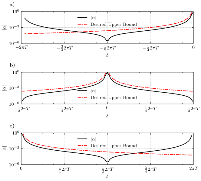
Figure 2: $\lvert\alpha\rvert$ versus $\delta$ for a) small eigenvalue $\frac{T-1}{T}\frac{1}{\kappa}$, b) moderate eigenvalue $\frac{T-1}{2T}$, and c) large eigenvalue $\frac{T-1}{T}$ with $t_{0}=2\pi T,T=\kappa+1.$

This issue can be avoided by choosing a $t_{0}$ strictly smaller than $2\pi T$, preserving (19), a maneuver with the side effect of wasting some range of the clock register. To explain, let us consider the choice of $t_{0}=\pi T$, in which case the approximated eigenvalues are

$$\tilde{\lambda}_{k}=2\frac{k}{T}=0,2\frac{1}{T},2\frac{2}{T},\cdots.$$ (21)

Hence, the values of $k$ from $0$ to $\left\lceil(T-1)/2\right\rceil$ is sufficient to cover the entire range of the true eigenvalues. For the problematic smallest and largest eigenvalues which made $\lvert\alpha\rvert$ violate the desired upper bound in Figure 2, with the new choice of $t_{0}=\pi T$, when $k$ is in the range from $\left\lceil(T-1)/2\right\rceil$ to $T-1$, the plot of $\lvert\alpha\rvert$ folds to the symmetric counterpart, confined to the desired upper bound. This behavior of $\lvert\alpha\rvert$ versus $\delta$ is visualized in Figure 3 with the same three examples of $\lambda_{j}$ as in Figure 2. Note that in addition to $t_{0}=\pi T$ satisfying condition (19), condition (20) requires that $T\geq 2\kappa+1$. In Figure 3, this choice is made as $T=\left\lceil 2\kappa+1\right\rceil$. One can observe that the desired upper bound is not violated in the entire range of $k$, regardless of the actual eigenvalue.

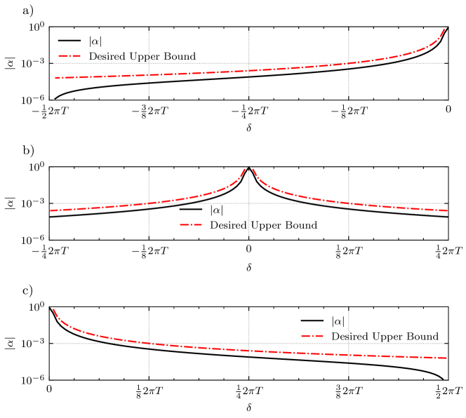
Figure 3: Data similarly illustrated as in Figure 2 with $t_{0}=\pi T,T=2\kappa+1$.

Choosing $t_{0}=\pi T$ can be effectively regarded as that the clock register range is not fully used. This “waste” of the clock register is necessary to truncate half of the period of $\lvert\alpha\rvert$, removing the unwanted tail on the opposite side when the actual eigenvalue $\lambda_{j}$ is close to either side of the boundary. More generally, choosing $t_{0}=\gamma(2\pi T)$ with $\gamma<\frac{1}{2}$ will utilize less spectrum while truncating the $\lvert\alpha\rvert$ more. A smaller $\gamma$ results in a smaller $t_{0}$, namely a faster Hamiltonian simulation Berry et al. (2007); Childs (2010), hence would be favorable. However, note that a small $\gamma$ would result in a larger $T$: according to (20), $T\geq\kappa/\gamma+1$. In other words, a shorter Hamiltonian simulation comes at a cost of requiring a larger clock register.

In summary, the above analysis on the amplitude behavior suggests that $t_{0}$ is $T$ multiplying a coefficient, where $T$ has lower bound inversely proportional to this coefficient, and proportional to the condition number. In the next section of the error analysis, which is built on the amplitude analysis in this section. The error will be proved to be bounded by $O(\kappa/t_{0})$. Hence, in practice, to achieve an error level of $\epsilon$, $t_{0}$ is chosen according to $O(\kappa/\epsilon)$ and so is $T$. When the matrix is ill-conditioned, a large clock register size $T$ and long Hamiltonian simulation time $t_{0}$ is required to maintain accuracy.

4 Error Analysis

The supplemental material accompanied with the original paper Harrow et al. (2009) established a through error analysis of the error propagation of the algorithm (though with some critical typos and misuses of notations that may cause confusion). We perform a rigrous error analysis in this section following the framework presented in Harrow et al. (2009).

Since we have defined $QC_{ideal}$ and $QC_{practical}$ in Section 2, we can use $QC_{ideal}$ as a benchmark to evaluate the error behavior of $QC_{practical}$. As a preview, the claims we make from the error analysis are summarized as the following theorem:

Theorem 1 (The HHL Error Bound).

1. The error between the ideal final state $\ket{\bar{\Phi}_{f}}$ and the actual final state $\ket{\Phi}_{f}$ is bounded as

   $$\lVert\ket{\Phi_{f}}-\ket{\bar{\Phi}_{f}}\rVert=O(\kappa/t_{0}).$$ (22)

2. If we post-select on the flag register being in the space spanned by $\{\ket{well},\ket{ill}\}$, and define the normalized state of register $I$ as $\ket{\bar{x}}$ in $QC_{ideal}$ and $\ket{x}$ in $QC_{practical}$, then

   $$\lVert\ket{x}-\ket{\bar{x}}\rVert=O(\kappa/t_{0}).$$ (23)

3. If $\ket{b}$ belongs to the well-conditioned subspace of $A$, and we post-select on $\ket{well}$ state of the flag register, then with the same definitions for $\ket{\bar{x}}$ and $\ket{x}$ as in the last case,

   $$\lVert\ket{x}-\ket{\bar{x}}\rVert=O(\kappa/t_{0}).$$ (24)

We use the next three subsections to prove the three claims in Theorem 1.

4.1 Proof of (22): Error Bound in the Final State Without Post-Selection

From linear algebra, the $L_{2}$ norm of the difference between any two arbitrary quantum states $\ket{\varphi_{1}}$ and $\ket{\varphi_{2}}$ is computed as

$$\lVert\ket{\varphi_{1}}-\ket{\varphi_{2}}\rVert=\sqrt{2(1-\Re\{\braket{\varphi_{1}}{\varphi_{2}}\})}.$$ (25)

In particular,

$$\lVert\ket{\Phi_{f}}-\ket{\bar{\Phi}_{f}}\rVert=\sqrt{2(1-\Re\{\braket{\Phi_{f}}{\bar{\Phi}_{f}}\})}$$ (26)

Hence, finding the upper bound of the error $\lVert\ket{\Phi_{f}}-\ket{\bar{\Phi}}_{f}\rVert$ amounts to finding the lower bound of $\Re\{\braket{\Phi_{f}}{\bar{\Phi}_{f}}\}$. We analyze the inner product as follows.

Note that (14) is inverse QPE operating on (13):

$$\ket{\Phi_{f}}=P^{\dagger}\sum_{j=1}^{N}\beta_{j}\ket{u_{j}}_{I}\sum_{k=0}^{T-1}\alpha_{k|j}\ket{k}_{C}\ket{h(\tilde{\lambda}_{k})}_{S}.$$ (27)

From (27) and (15) and some manipulations, one can derive that

$$\braket{\Phi_{f}}{\bar{\Phi}_{f}}=\sum_{j=0}^{N-1}\sum_{k=0}^{T-1}\lvert\beta_{j}\rvert^{2}\lvert\alpha_{k|j}\rvert^{2}\braket{h(\tilde{\lambda}_{k})}{h(\lambda_{j})}\in\mathbb{R}.$$ (28)

To explain why this inner product is a real number, we note that as the matrix $A$ is Hermitian, its eigenvalue $\lambda_{j}\in\mathbb{R}$. The approximated eigenvalue $\tilde{\lambda}_{k}\in\mathbb{R}$ according to (7). The mapping $f,g$ are both $\mathbb{R}\to\mathbb{R}$, which renders every amplitude in $\ket{h(\lambda)}$ real. As a result, $\braket{h(\tilde{\lambda}_{k})}{h(\lambda_{j})}\in\mathbb{R}$, and (28) is real. The real part of the inner product (28) can be separated into two parts:

$$\Re\{\braket{\Phi_{f}}{\bar{\Phi}_{f}}\}=\braket{\Phi_{f}}{\bar{\Phi}_{f}}=\underbrace{\sum_{j=0}^{N-1}\sum_{k:\lvert\delta\rvert\leq 2\pi}\lvert\beta_{j}\rvert^{2}\lvert\alpha_{k|j}\rvert^{2}\braket{h(\tilde{\lambda}_{k})}{h(\lambda_{j})}}_{\text{Term 1}}+\underbrace{\sum_{j=0}^{N-1}\sum_{k:\lvert\delta\rvert>2\pi}\lvert\beta_{j}\rvert^{2}\lvert\alpha_{k|j}\rvert^{2}\braket{h(\tilde{\lambda}_{k})}{h(\lambda_{j})}}_{\text{Term 2}}.$$ (29)

according to the condition

$$k:\lvert\delta\rvert\leq 2\pi\Longleftrightarrow\lvert k-\frac{t_{0}}{2\pi}\lambda_{j}\rvert\leq 1.$$ (30)

Condition (30) being satisfied means that the approximated eigenvalue $\tilde{\lambda}_{k}$ is in the direct proximity of the true eigenvalue $\lambda_{j}$: only values of $k$ that satisfy (30) are $\left\lceil\frac{t_{0}}{2\pi}\lambda_{j}\right\rceil$, $\left\lfloor\frac{t_{0}}{2\pi}\lambda_{j}\right\rfloor$, and possibly $\frac{t_{0}}{2\pi}\lambda_{j}$ itself if it is an integer. Hence, Term 1 and Term 2 correspond to the error contribution from good and poor eigenvalue approximations, respectively.

Next, we seek the lower bounds for both Term 1 and Term 2 to lower bound $\Re{\braket{\tilde{\varphi}}{\varphi}}$. To this end, we need to find the lower bound for $\Re\{\braket{h(\tilde{\lambda}_{k})}{h(\lambda_{j})}\}=\braket{h(\tilde{\lambda}_{k})}{h(\lambda_{j})}$, a result that can be directly derived from the following Lemma 2.

Lemma 2 (The continuity of the mapping $\lambda\to\ket{h(\lambda)}$).

The mapping $\lambda\to\ket{h(\lambda)}$ is $O(\kappa)$-Lipschitz. Namely, for any $\lambda_{1}\neq\lambda_{2}$,

$$\lVert\ket{h(\lambda_{1})}-\ket{h(\lambda_{2})}\rVert\leq c\kappa\lvert\lambda_{1}-\lambda_{2}\rvert,$$ (31)

where $c=O(1)$ is a constant.

From (25) and (31), we have

$$\lVert\ket{h(\tilde{\lambda}_{k})}-\ket{h(\lambda_{j})}\rVert=\sqrt{2(1-\Re\braket{h(\tilde{\lambda}_{k})}{h(\lambda_{j})})}\leq c\kappa\lvert\tilde{\lambda}_{k}-\lambda_{j}\rvert,$$ (32)

which yields

$$\Re\braket{h(\tilde{\lambda}_{k})}{h(\lambda_{j})}\geq 1-\frac{1}{2}c^{2}\kappa^{2}(\tilde{\lambda}_{k}-\lambda_{j})^{2}=1-\frac{c^{2}}{2}\frac{\kappa^{2}}{t_{0}^{2}}\delta^{2}.$$ (33)

With (33), one can prove that

Term 1 $$\coloneqq\sum_{j=0}^{N-1}\sum_{k:\lvert\delta\rvert\leq 2\pi}\lvert\beta_{j}\rvert^{2}\lvert\alpha_{k|j}\rvert^{2}\Re{\braket{h(\tilde{\lambda}_{k})}{h(\lambda_{j})}}$$ (34)

$$\geq\sum_{j=0}^{N-1}\sum_{k:\lvert\delta\rvert\leq 2\pi}\lvert\beta_{j}\rvert^{2}\lvert\alpha_{k|j}\rvert^{2}-\frac{c^{2}}{2}\frac{\kappa^{2}}{t_{0}^{2}}\sum_{j=0}^{N-1}\sum_{k:\lvert\delta\rvert\leq 2\pi}\lvert\beta_{j}\rvert^{2}\lvert\alpha_{k|j}\rvert^{2}\delta^{2}$$ (35)

$$\geq\sum_{j=0}^{N-1}\sum_{k:\lvert\delta\rvert\leq 2\pi}\lvert\beta_{j}\rvert^{2}\lvert\alpha_{k|j}\rvert^{2}-2\pi^{2}c^{2}\frac{\kappa^{2}}{t_{0}^{2}}$$ (36)

To bound Term 2, another fact we need is that $\lvert\alpha_{k|j}\rvert$ is upper bounded when $\delta$ is large, i.e., when the eigenvalue approximation is poor. In Section 3, it has been shown numerically that $\lvert\alpha_{k|j}\rvert$ is bounded by

$$\lvert\alpha_{k|j}\rvert<\frac{8\pi}{\delta^{2}}\quad\text{if}\quad\lvert\delta\rvert>2\pi.$$ (37)

The analytical proof of (37) is provided in Appendix D.

Based on (33) and (37), we have

Term 2 $$\coloneqq\sum_{j=0}^{N-1}\sum_{k:\lvert\delta\rvert>2\pi}\lvert\beta_{j}\rvert^{2}\lvert\alpha_{k|j}\rvert^{2}\Re{\braket{h(\tilde{\lambda}_{k})}{h(\lambda_{j})}}$$ (38)

$$\geq\sum_{j=0}^{N-1}\sum_{k:\lvert\delta\rvert>2\pi}\lvert\beta_{j}\rvert^{2}\lvert\alpha_{k|j}\rvert^{2}-\frac{c^{2}\kappa^{2}}{2t_{0}^{2}}\sum_{j=0}^{N-1}\sum_{k:\lvert\delta\rvert>2\pi}\lvert\beta_{j}\rvert^{2}\lvert\alpha_{k|j}\rvert^{2}\delta^{2}$$ (39)

$$\geq\sum_{j=0}^{N-1}\sum_{k:\lvert\delta\rvert>2\pi}\lvert\beta_{j}\rvert^{2}\lvert\alpha_{k|j}\rvert^{2}-\frac{32\pi^{2}c^{2}\kappa^{2}}{t_{0}^{2}}\sum_{j=0}^{N-1}\sum_{k:\lvert\delta\rvert>2\pi}\lvert\beta_{j}\rvert^{2}\frac{1}{\delta^{2}}$$ (40)

$$\geq\sum_{j=0}^{N-1}\sum_{k:\lvert\delta\rvert>2\pi}\lvert\beta_{j}\rvert^{2}\lvert\alpha_{k|j}\rvert^{2}-\frac{4\pi^{2}c^{2}\kappa^{2}}{3t_{0}^{2}}$$ (41)

where we used

$$\sum_{j=0}^{N-1}\lvert\beta_{j}\rvert^{2}\sum_{k:\lvert\delta\rvert>2\pi}\frac{1}{\delta_{k|j}^{2}}\leq\frac{1}{24}$$ (42)

to get from (40) to (41).

From (36), (41), and (29), we have

$$\Re\{\braket{\Phi_{f}}{\bar{\Phi}_{f}}\}\geq 1-\frac{10\pi^{2}c^{2}}{3}\frac{\kappa^{2}}{t_{0}^{2}}.$$ (43)

Plugging (43) back into (26), we have completed the proof for claim (22).

$$\lVert\ket{\Phi_{f}}-\ket{\bar{\Phi}_{f}}\rVert\leq\sqrt{\frac{20}{3}}\pi c\frac{\kappa}{t_{0}}=O(\frac{\kappa}{t_{0}}).$$ (44)

4.2 Proof of (23): Error Bound in the Solution State with Flag Register Post-Selected in $\{\ket{well},\ket{ill}\}$

The post-selection is introduced in Section 2. From the ideal and non-ideal final states (15) and (14), the post-selection onto the $\{\ket{well},\ket{ill}\}$ subspace of the flag register results in the ideal and non-ideal solution states

$$\ket{\bar{x}}=\frac{1}{\sqrt{\bar{p}}}\sum_{j=0}^{N-1}\beta_{j}\ket{u_{j}}\left[f(\lambda_{j})\ket{well}+g(\lambda_{j})\ket{ill}\right],$$ (45)

$$\ket{x}=\frac{1}{\sqrt{p}}P^{\dagger}\sum_{j=0}^{N-1}\beta_{j}\ket{u_{j}}\sum_{k=0}^{T-1}\alpha_{k|j}\ket{k}\left[f(\tilde{\lambda}_{k})\ket{well}+g(\tilde{\lambda}_{k})\ket{ill}\right],$$ (46)

where the post-selection success probabilities are

$$\bar{p}=\sum_{j=0}^{N-1}\lvert\beta_{j}\rvert^{2}\left[f^{2}(\lambda_{j})+g^{2}(\lambda_{j})\right],$$ (47)

and

$$p=\sum_{j=0}^{N-1}\lvert\beta_{j}\rvert^{2}\sum_{k=0}^{T-1}\lvert\alpha_{k|j}\rvert^{2}\left[f^{2}(\tilde{\lambda}_{k})+g^{2}(\tilde{\lambda}_{k})\right].$$ (48)

The inner product between states $\ket{\bar{x}}$ and $\ket{x}$ is thus

$$\braket{x}{\bar{x}}=\frac{1}{\sqrt{p\bar{p}}}\sum_{j=0}^{N-1}\lvert\beta_{j}\rvert^{2}\sum_{k=0}^{T-1}\lvert\alpha_{k|j}\rvert^{2}\left[f(\tilde{\lambda}_{k})f(\lambda_{j})+g(\tilde{\lambda}_{k})g(\lambda_{j})\right].$$ (49)

Note that $\braket{x}{\bar{x}}$ is real, hence,

$$\braket{x}{\bar{x}}=\braket{\bar{x}}{x}=\Re\{\braket{x}{\bar{x}}\}=\Re\{\braket{\bar{x}}{x}\}.$$ (50)

To simplify the notation, we introduce the following definitions:

$$f_{j}\coloneqq f(\lambda_{j}),\qquad\tilde{f}_{k}\coloneqq f(\tilde{\lambda}_{k}),$$ (51)

$$g\coloneqq g(\lambda_{j}),\qquad\tilde{g}\coloneqq g(\tilde{\lambda}_{k}).$$ (52)

Furthermore, we treat $\lvert\beta_{j}\rvert^{2}$ and $\lvert\alpha_{k|j}\rvert^{2}$ as distributions and introduce the expectation functions

$$\mathbb{E}(X_{j})=\sum_{j=0}^{N-1}\lvert\beta_{j}\rvert^{2}X_{j},$$ (53)

$$\mathbb{E}(X_{k,j})=\sum_{j=0}^{N-1}\lvert\beta_{j}\rvert^{2}\sum_{k=0}^{T-1}\lvert\alpha_{k|j}\rvert^{2}X_{k,j},$$ (54)

where $X_{j}$ and $X_{k,j}$ are random variables. Therefore, equations (47) to (49) can be represented as the expectations as

$$\bar{p}=\mathbb{E}(f_{j}^{2}+g_{j}^{2}),\qquad p=\mathbb{E}(\tilde{f}_{k}^{2}+\tilde{g}_{k}^{2}),\qquad F =\frac{1}{\sqrt{p\bar{p}}}\mathbb{E}\left(\tilde{f}_{k}f_{j}+\tilde{g}_{k}g_{j}\right).$$ (55)

With more derivation details included in the Appendix, (49) is lower bounded as

$$\braket{x}{\bar{x}} =\frac{1}{\sqrt{p\bar{p}}}\mathbb{E}\left(\tilde{f}_{k}f_{j}+\tilde{g}_{k}g_{j}\right)=\frac{1+\mathbb{E}\left((\tilde{f}_{k}-f_{j})f_{j}+(\tilde{g}_{k}-g_{j})g_{j}\right)/\bar{p}}{\sqrt{1+\frac{p-\bar{p}}{\bar{p}}}}$$ (56)

$$\geq\left[1+\mathbb{E}\left[(\tilde{f}_{k}-f_{j})f_{j}+(\tilde{g}_{k}-g_{j})g_{j}\right]/\bar{p}\right]\left(1-\frac{1}{2}\frac{p-\bar{p}}{\bar{p}}\right)$$ (57)

$$\geq 1-\underbrace{\frac{1}{2\bar{p}}\mathbb{E}\left[(\tilde{f}_{k}-f_{j})^{2}+(\tilde{g}_{k}-g_{j})^{2}\right]}_{\text{Term 1}}-\underbrace{\frac{1}{2}\frac{p-\bar{p}}{\bar{p}^{2}}\mathbb{E}\left[(\tilde{f}_{k}-f_{j})f_{j}+(\tilde{g}_{k}-g_{j})g_{j}\right]}_{\text{Term 2}}.$$ (58)

Next, the upper bounds of Term 1 and Term 2 are studied to yield the lower bound of $\braket{x}{\bar{x}}$. One important prerequisite for this study is the behavior of the filter functions, which is given in Lemma 3, whose proof is provided in the Appendix.

Lemma 3 (Upper bound of $(\tilde{f}_{k}-f_{j})^{2}+(\tilde{g}_{k}-g_{j})^{2}$).

$$(\tilde{f}_{k}-f_{j})^{2}+(\tilde{g}_{k}-g_{j})^{2}=O\left(\frac{\kappa^{2}}{t_{0}^{2}}\delta_{k|j}^{2}(f_{j}^{2}+g_{j}^{2})\right).$$ (59)

Applying Lemma 3 to the expectation in Term 1 gives

$$\mathbb{E}\left[(\tilde{f}_{k}-f_{j})^{2}+(\tilde{g}_{k}-g_{j})^{2}\right]=O\left(\frac{\kappa^{2}}{t_{0}^{2}}\mathbb{E}\left[\delta_{k|j}^{2}(f_{j}^{2}+g_{j}^{2})\right]\right).$$ (60)

Using (55), Term 1 becomes

$$\text{Term 1}=\frac{1}{2\bar{p}}\mathbb{E}\left[(\tilde{f}_{k}-f_{j})^{2}+(\tilde{g}_{k}-g_{j})^{2}\right]=O\left(\frac{\kappa^{2}}{t_{0}^{2}}\frac{\mathbb{E}\left[\delta_{k|j}^{2}(f_{j}^{2}+g_{j}^{2})\right]}{\mathbb{E}(f_{j}^{2}+g_{j}^{2})}\right),$$ (61)

in which the ratio between the expectations is

$$\frac{\mathbb{E}\left[\delta_{k|j}^{2}(f_{j}^{2}+g_{j}^{2})\right]}{\mathbb{E}(f_{j}^{2}+g_{j}^{2})}=\frac{\sum_{j=0}^{N-1}\lvert\beta_{j}\rvert^{2}(f_{j}^{2}+g_{j}^{2})\sum_{k=0}^{T-1}\lvert\alpha_{k|j}^{2}\rvert\delta_{k|j}^{2}}{\sum_{j=0}^{N-1}\lvert\beta_{j}\rvert^{2}(f_{j}^{2}+g_{j}^{2})}.$$ (62)

In the appendix, it is proved that $\mathbb{E}(\delta_{k|j}^{2})=O(1)$. Subsequently, $\sum_{k=0}^{T-1}\lvert\alpha_{k|j}^{2}\rvert\delta_{k|j}^{2}$ is also $O(1)$. Hence, the ratio (62) is $O(1)$ as it is a weighted sum. This concludes that Term 1 (61) is $O(\kappa^{2}/t_{0}^{2})$.

Transitioning to the examination of Term 2, first we note that

$$\mathbb{E} \left[(\tilde{f}_{k}-f_{j})f_{j}+(\tilde{g}_{k}-g_{j})g_{j}\right]\leq\mathbb{E}\left[\lvert(\tilde{f}_{k}-f_{j})f_{j}+(\tilde{g}_{k}-g_{j})g_{j}\rvert\right]$$ (63)

$$\leq\mathbb{E}\left[\sqrt{(\tilde{f}_{k}-f_{j})^{2}+(\tilde{g}_{k}-g_{j})^{2}}\sqrt{f_{j}^{2}+g_{j}^{2}}\right]=O\left(\frac{\kappa}{t_{0}}\mathbb{E}\left[\lvert\delta_{k|j}\rvert(f_{j}^{2}+g_{j}^{2})\right]\right)$$ (64)

where we have used the fact that $(\tilde{f}_{k}-f_{j})f_{j}+(\tilde{g}_{k}-g_{j})g_{j}$ is not necessary positive, Cauchy-Schwartz inequality, and Lemma 3 in sequence in the derivation above. Given that $\mathbb{E}(\lvert\delta_{k|j}\rvert)=O(1)$, we find that

$$\frac{\mathbb{E}\left[(\tilde{f}_{k}-f_{j})f_{j}+(\tilde{g}_{k}-g_{j})g_{j}\right]}{\bar{p}}=O\left(\frac{\kappa}{t_{0}}\frac{\mathbb{E}\left[\lvert\delta_{k|j}\rvert(f_{j}^{2}+g_{j}^{2})\right]}{\mathbb{E}(f_{j}^{2}+g_{j}^{2})}\right)=O\left(\frac{\kappa}{t_{0}}\right)$$ (65)

in Term 2. The other multiplier of Term 2 is

$$\frac{p-\bar{p}}{\bar{p}} =\frac{\mathbb{E}\left[(\tilde{f}_{k}-f_{j})^{2}+(\tilde{g}_{k}-g_{j})^{2}\right]+2\mathbb{E}\left[(\tilde{f}_{k}-f_{j})f_{j}+(\tilde{g}_{k}-g_{j})g_{j}\right]}{\mathbb{E}(f_{j}^{2}+g_{j}^{2})}$$ (66)

$$=O\left(\frac{\kappa^{2}}{t_{0}^{2}}\frac{\mathbb{E}\left[\delta_{k|j}^{2}(f_{j}^{2}+g_{j}^{2})\right]}{\mathbb{E}(f_{j}^{2}+g_{j}^{2})}\right)+O\left(\frac{\kappa}{t_{0}}\frac{\mathbb{E}\left[\lvert\delta_{k|j}\rvert(f_{j}^{2}+g_{j}^{2})\right]}{\mathbb{E}\left[(f_{j}^{2}+g_{j}^{2})\right]}\right)$$ (67)

$$=O\left(\frac{\kappa^{2}}{t_{0}^{2}}\mathbb{E}\left(\delta_{k|j}^{2}\right)\right)+O\left(\frac{\kappa}{t_{0}}\mathbb{E}\left(\lvert\delta_{k|j}\rvert\right)\right)=O\left(\frac{\kappa^{2}}{t_{0}^{2}}\right)+O\left(\frac{\kappa}{t_{0}}\right).$$ (68)

Recall that $t_{0}=\Omega(\kappa)$ from Section 3, leading to the fact that $\kappa/t_{0}<1$, plugging which to (68) yields

$$\frac{p-\bar{p}}{\bar{p}}=O\left(\frac{\kappa}{t_{0}}\right).$$ (69)

Term 2 is the product of (65) and (69), hence, Term 2 is $O(\kappa^{2}/t_{0}^{2})$. At this point, we have proved that both Term 1 and Term 2 are $O(\kappa^{2}/t_{0}^{2})$. Subsequently from (58),

$$\braket{x}{\bar{x}}=1-O\left(\frac{\kappa^{2}}{t_{0}^{2}}\right).$$ (70)

Using (25), we have

$$\lVert\ket{x}-\ket{\bar{x}}\rVert=\sqrt{2(1-\Re\{\braket{x}{\bar{x}}\})}=O\left(\frac{\kappa}{t_{0}}\right).$$ (71)

4.3 Proof of (24): Error Bound in the Solution State with Flag Register Post-Selected in $\{\ket{well}\}$

To utilize the analysis performed in Sections 4.1 and 4.2, we regard the process of obtaining the solution state as first post selecting the flag register on the subspace of $\{\ket{well},\ket{ill}\}$, followed by another post selection on to $\{\ket{well}\}$. We denote these two post selection operators as $PS_{1}$ and $PS_{2}$. As the phase register does not entangle with other registers in the final state, in this section, we omit it in all representations.

When $\ket{b}$ stays in the well-conditioned subspace of $A$, i.e., $\ket{b}$ is a linear combination of eigenvalues of $A$ whose eigenvalues are in $\left[\frac{1}{\tilde{\kappa}},1\right]$, the ideal final state $\ket{\bar{\Phi}_{f}}$ would have no $\ket{ill}$ and $\ket{nothing}$ components in the flag register

$$\ket{\bar{\Phi}_{f}}=A^{-1}\ket{b}\ket{well}.$$ (72)

Thus, both post-selections have the success probability of 1.

$$\ket{\bar{x}_{1}}\coloneqq PS_{1}\ket{\bar{\Phi}_{f}}=A^{-1}\ket{b}\ket{well},$$ (73)

$$\ket{\bar{x}_{2}}\coloneqq PS_{2}\ket{\bar{x}_{1}}=A^{-1}\ket{b}\ket{well},$$ (74)

and the solution state is

$$\ket{\bar{x}}=A^{-1}\ket{b}.$$ (75)

The non-ideal case final state contains components in all three subspaces of the flag register spanned by its basis states $\{\ket{well}\}$, $\{\ket{ill}\}$, $\{\ket{nothing}\}$:

$$\ket{\Phi_{f}}=\mathbf{x}_{f}^{w}\ket{well}+\mathbf{x}_{f}^{i}\ket{ill}+\mathbf{x}_{f}^{n}\ket{nothing}.$$ (76)

$PS_{1}$ succeeds with the probability $p_{1}=\lVert\mathbf{x}_{f}^{w}\rVert^{2}+\lVert\mathbf{x}_{f}^{i}\rVert^{2}$ and yields

$$\ket{x_{1}}\coloneqq PS_{1}{\ket{\Phi_{f}}}=\mathbf{x}_{1}^{w}\ket{well}+\mathbf{x}_{1}^{i}\ket{ill},\quad\mathbf{x}_{1}^{w}=\mathbf{x}_{f}^{w}/\sqrt{p_{1}},\quad\mathbf{x}_{1}^{i}=\mathbf{x}_{f}^{i}/\sqrt{p_{1}}$$ (77)

Similarly, $PS_{2}$ succeeds with the probability $p_{2}=\lVert\mathbf{x}_{1}^{w}\rVert^{2}$ and yields

$$\ket{x_{2}}\coloneqq PS_{2}{\ket{x_{1}}}=\ket{x}\ket{well},\quad\ket{x}=\mathbf{x}_{1}^{w}/\sqrt{p_{2}}.$$ (78)

From Section 4.2, we know that

$$\Re\{\braket{x_{1}}{\bar{x}_{1}}\}=1-O\left(\frac{\kappa^{2}}{t_{0}^{2}}\right)$$ (79)

holds in general. Within the context of this section, i.e., (73), (75), (77),

$$\braket{x_{1}}{\bar{x}_{1}}=(\mathbf{x}_{1}^{w})^{\dagger}\ket{\bar{x}}.$$ (80)

Combining (79) and (80) gives

$$\Re\{\braket{x_{1}}{\bar{x}_{1}}\}=\Re\{(\mathbf{x}_{1}^{w})^{\dagger}\ket{\bar{x}}\}=1-O\left(\frac{\kappa^{2}}{t_{0}^{2}}\right).$$ (81)

Similar to previous subsections, we rely on (25) and prove the upper bound for $\lVert\ket{x}-\ket{\bar{x}}\rVert$ by finding the lower bound for $\Re\{\braket{x}{\bar{x}}\}$. The latter is given as

$$\Re\{\braket{x}{\bar{x}}\}=\frac{1}{\sqrt{p_{2}}}\Re\{(\mathbf{x}_{1}^{w})^{\dagger}\ket{\bar{x}}\}=\frac{1}{\sqrt{p_{2}}}-O\left(\frac{\kappa^{2}}{t_{0}^{2}}\right)>1-O\left(\frac{\kappa^{2}}{t_{0}^{2}}\right),$$ (82)

where we have used (78), (81), and the fact that $p_{2}<1$. Physically, (82) means that the second post-selection amplifies the error by $1/\sqrt{p_{2}}$, however, this does not affect the overall error scaling. Plugging (82) into (25) completes the proof of (24).

4.4 Summary

To summarize the error analysis, all claims are proved by finding the lower bound for the real part of the inner product between the ideal and non-ideal states. The inner product for the final state is studied by separating the contributions from good and bad eigenvalue approximations. The post-selection error to $\{\ket{well},\ket{ill}\}$ subspace is bounded by expressing the division by the success probability as a weighted sum. When projecting to the $\{\ket{well}\}$ subspace, the proof is finalized by straightforwardly applying the previous analysis. In practice, the error bound provides the instruction on the selection on $t_{0}$ to achieve a prescribed target error level $\epsilon$: choosing $t_{0}=O(\kappa/\epsilon)$. Note that this choice adheres to the choice we discussed in Section 3: $t_{0}=\gamma(2\pi T)$, $T\geq\kappa/\gamma+1$ with $\gamma<1/2$.

5 Conclusion

A detailed error analysis of the HHL algorithm is presented in this work. Besides offering corrections to mistakes, compared with the supplementary material of Harrow et al. (2009), this analysis covers derivation details with explicit expressions to be more approachable. The connection between the Hamiltonian simulation duration $t_{0}$ and the clock register size $T$ is also established as a result of the analysis of the amplitudes after QPE, without assuming an infinite $T$ as in Harrow et al. (2009). We hope this work would be useful to those who try to discover improved version of the HHL algorithm when an error analysis is needed for the derived algorithm.

Appendix A The inner product between ideal and non-ideal final states

Based on the definition of QPE $P$ in Section 2, it operating on $\ket{\Phi_{f}}$ (15) would yield

$$P\ket{\bar{\Phi}_{f}}=\sum_{j=0}^{N-1}\beta_{j}\ket{u_{j}}\sum_{k=0}^{T-1}\alpha_{k|j}\ket{k}\ket{h(\lambda_{j})}.$$ (83)

Hence,

$$\braket{\Phi_{f}}{\bar{\Phi}_{f}} =\braket{\Phi_{f}}{P^{\dagger}P}{\bar{\Phi}}$$ (84)

$$=\left(\sum_{j=0}^{N}\beta_{j}^{*}\bra{u_{j}}\sum_{k=0}^{T-1}\alpha_{k|j}^{*}\bra{k}\bra{h(\tilde{\lambda}_{k})}\right)\left(\sum_{j^{\prime}=0}^{N-1}\beta_{j^{\prime}}\ket{u_{j^{\prime}}}\sum_{k^{\prime}=0}^{T-1}\alpha_{k^{\prime}|j^{\prime}}\ket{k^{\prime}}\ket{h(\lambda_{j^{\prime}})}\right)$$ (85)

$$=\sum_{j=0}^{N-1}\sum_{k=0}^{T-1}\lvert\beta_{j}\rvert^{2}\lvert\alpha_{k|j}\rvert^{2}\braket{h(\tilde{\lambda}_{k})}{h(\lambda_{j})}$$ (86)

Appendix B The mapping $\lambda\to\ket{h(\lambda)}$ is $O(\kappa)$-Lipschitz.

B.1 Model $\ket{h(\lambda)}$ as a Vector-Valued Function

Suppose a vector-valued function

$$\mathbf{f}(t)=\begin{bmatrix}x(t)\\ y(t)\\ z(t)\end{bmatrix},$$ (87)

is defined in $t\in[t_{L},t_{R}]$, and each component $x(t),y(t)$, and $z(t)$ is differentiable in $(t_{L},t_{R})$ except at two points $t_{1}$ and $t_{2}$ with $t_{L}<t_{1}<t_{2}<t_{R}$. We aim to find a upper bound of the value

$$\frac{\lVert\mathbf{f}(t_{l})-\mathbf{f}(t_{r})\rVert^{2}}{\lvert t_{l}-t_{r}\rvert^{2}}=\frac{(x(t_{l})-x(t_{r}))^{2}}{(t_{l}-t_{r})^{2}}+\frac{(y(t_{l})-y(t_{r}))^{2}}{(t_{l}-t_{r})^{2}}+\frac{(z(t_{l})-z(t_{r}))^{2}}{(t_{l}-t_{r})^{2}}$$ (88)

for arbitrary two points $t_{l}<t_{r}$ from $[t_{L},t_{R}]$.

If both $t_{l}$ and $t_{r}$ are contained in a single domain from the set $S=\{[t_{L},t_{1}),(t_{1},t_{2}),(t_{2},t_{R}]\}$, we apply the mean-value theorem and obtain that

$$\frac{\lVert\mathbf{f}(t_{l})-\mathbf{f}(t_{r})\rVert^{2}}{\lvert t_{l}-t_{r}\rvert^{2}} =\frac{(x(t_{l})-x(t_{r}))^{2}}{(t_{l}-t_{r})^{2}}+\frac{(y(t_{l})-y(t_{r}))^{2}}{(t_{l}-t_{r})^{2}}+\frac{(z(t_{l})-z(t_{r}))^{2}}{(t_{l}-t_{r})^{2}}$$ (89)

$$=[x^{\prime}(c_{1})]^{2}+[y^{\prime}(c_{2})]^{2}+[z^{\prime}(c_{3})]^{2},$$ (90)

where $c_{1},c_{2}$, and $c_{3}$ are some constants in $(t_{l},t_{r})$, and the superscript prime denotes derivative. Equation (90) suggests that

$$\frac{\lVert\mathbf{f}(t_{l})-\mathbf{f}(t_{r})\rVert^{2}}{\lvert t_{l}-t_{r}\rvert^{2}}\leq\max_{t\in(t_{l},t_{r})}[x^{\prime}(t)]^{2}+\max_{t\in(t_{l},t_{r})}[y^{\prime}(t)]^{2}+\max_{t\in(t_{l},t_{r})}[z^{\prime}(t)]^{2}.$$ (91)

Now let us consider the case when $t_{l}$ and $t_{r}$ belong to different domains from the set $S$. Suppose $t_{l}$ and $t_{r}$ are from two adjacent domains in $S$. We symbolize the disconnecting point of the two domains as $t_{c}$. Then applying the mean value theorem in regions $(t_{l},t_{c})$ and $(t_{c},t_{r})$ to $x(t)$ gives

$$x(t_{r})-x(t_{c})=(t_{r}-t_{c})x^{\prime}(c_{1}),$$ (92)

$$x(t_{c})-x(t_{l})=(t_{c}-t_{l})x^{\prime}(c_{2}).$$ (93)

As a result,

$$\lvert x(t_{r})-x(t_{l})\rvert =\lvert x(t_{r})-x(t_{c})+x(t_{c})-x(t_{l})\rvert$$ (94)

$$\leq\lvert x(t_{r})-x(t_{c})\rvert+\lvert x(t_{c})-x(t_{l})\rvert$$ (95)

$$=\lvert(t_{r}-t_{c})x^{\prime}(c_{1})\rvert+\lvert(t_{c}-t_{l})x^{\prime}(c_{2})\rvert$$ (96)

$$=(t_{r}-t_{c})\lvert x^{\prime}(c_{1})\rvert+(t_{c}-t_{l})\lvert x^{\prime}(c_{2})\rvert$$ (97)

$$\leq(t_{r}-t_{c})\max_{t\in(t_{c},t_{r})}{\lvert x^{\prime}(t)\rvert}+(t_{c}-t_{l})\max_{t\in(t_{l},t_{c})}{\lvert x^{\prime}(t)\rvert}$$ (98)

$$\leq(t_{r}-t_{l})\max_{t\in(t_{l},t_{r})}{\lvert x^{\prime}(t)\rvert}.$$ (99)

In other words,

$$\frac{\lvert x(t_{r})-x(t_{l})\rvert^{2}}{(t_{r}-t_{l})^{2}}\leq\max_{t\in(t_{l},t_{r})}[x^{\prime}(t)]^{2}.$$ (100)

Same procedure applies to $y(t)$ and $z(t)$. Hence,

$$\frac{\lvert y(t_{r})-y(t_{l})\rvert^{2}}{(t_{r}-t_{l})^{2}}\leq\max_{t\in(t_{l},t_{r})}[y^{\prime}(t)]^{2}.$$ (101)

$$\frac{\lvert z(t_{r})-z(t_{l})\rvert^{2}}{(t_{r}-t_{l})^{2}}\leq\max_{t\in(t_{l},t_{r})}[z^{\prime}(t)]^{2}.$$ (102)

Equation (88) together with (100), (101), (102) indicates that the upper bound equation (91) still holds in this case.

Following a similar procedure, one can prove that if $t_{l}$ and $t_{r}$ are not from adjacent domains in $S$, equation (91) also holds.

In summary, for arbitrary two points $t_{l}<t_{r}$ in domain $[t_{L},t_{R}]$, one upper bound for the value of interest expressed in equation (88) is given as equation (91).

B.2 The Study for the Mapping $\lambda\to\ket{h(\lambda)}$

Now let us study the mapping $\lambda\to\ket{h(\lambda)}$. It is clear from the definition (2) that $\ket{h(\lambda)}$ can be modeled as a vector-valued function defined on domain $[0,1]$, where the components $\sqrt{1-f^{2}(\lambda)-g^{2}(\lambda)}$, $f(\lambda)$, and $g(\lambda)$ are differentiable on $(0,\frac{1}{2\tilde{\kappa}})\cup(\frac{1}{2\tilde{\kappa}},\frac{1}{\tilde{\kappa}})\cup(\frac{1}{\tilde{\kappa}},1)$. Thus, the study from the last subsection applies to $\ket{h(\lambda)}$, leading to

$$\frac{\lVert\ket{h(\lambda_{2})}-\ket{h(\lambda_{1})}\rVert^{2}}{\lvert\lambda_{2}-\lambda_{1}\rvert^{2}} \leq\max_{\lambda\in(0,1)}\left[\frac{d}{d\lambda}\sqrt{1-f^{2}(\lambda)-g^{2}(\lambda)}\right]^{2}$$

$$\quad+\max_{\lambda\in(0,1)}\left[\frac{df(\lambda)}{d\lambda}\right]^{2}+\max_{\lambda\in(0,1)}\left[\frac{dg(\lambda)}{d\lambda}\right]^{2}$$ (103)

$$=\left[\frac{\tilde{\kappa}}{2\sqrt{3}}\right]^{2}+\left[\frac{\pi}{2}\tilde{\kappa}\right]^{2}+\left[\frac{\pi}{2}\tilde{\kappa}\right]^{2}=\frac{6\pi^{2}+1}{12}\tilde{\kappa}^{2}$$ (104)

for any $\lambda_{1}\neq\lambda_{2}$ in $[0,1]$. Hence,

$$\lVert\ket{h(\lambda_{2})}-\ket{h(\lambda_{1})}\rVert\leq\sqrt{\frac{6\pi^{2}+1}{12}}\tilde{\kappa}\lvert\lambda_{2}-\lambda_{1}\rvert.$$ (105)

Equation (105) together with (12) gives that

$$\lVert\ket{h(\lambda_{2})}-\ket{h(\lambda_{1})}\rVert=O(\kappa)\lvert\lambda_{2}-\lambda_{1}\rvert,$$ (106)

which completes the proof of Lemma 2. ∎

Additional note: We are not attempting to find the best upper bound for $\lVert\ket{h(\lambda_{2})}-\ket{h(\lambda_{1})}\rVert/\lvert\lambda_{2}-\lambda_{1}\rvert$ in the proof, rather simply prove that it is bounded by $O(\kappa)$. Tighter upper bound than the one in (105) may be found, but we note that the factor $\pi/2$ as claimed in Harrow et al. (2009) is not correct for certain values of $\kappa$.

Appendix C Simplified expressions of $\alpha_{k|j}$ and $\lvert\alpha_{k|j}\rvert$

$$\alpha_{k|j} =\frac{\sqrt{2}}{T}\sum_{\tau=0}^{T-1}\sin\left[\frac{\pi}{T}\left(\tau+\frac{1}{2}\right)\right]e^{i\left(\lambda_{j}-\frac{2\pi}{t_{0}}k\right)\frac{t_{0}}{T}\tau}$$ (107)

$$=\frac{\sqrt{2}}{T}\sum_{\tau=0}^{T-1}\sin\left[\frac{\pi}{T}\left(\tau+\frac{1}{2}\right)\right]e^{i\tau\delta/T}$$ (108)

$$=\frac{\sqrt{2}}{T}\frac{1}{2i}\sum_{\tau=0}^{T-1}\left[e^{i\frac{\pi}{T}\left(\tau+\frac{1}{2}\right)}-e^{-i\frac{\pi}{T}\left(\tau+\frac{1}{2}\right)}\right]e^{i\delta\tau/T}$$ (109)

$$=\frac{\sqrt{2}}{T}\frac{1}{2i}\left[e^{i\frac{\pi}{2T}}\sum_{\tau=0}^{T-1}e^{i\tau\left(\delta+\pi\right)/T}-e^{-i\frac{\pi}{2T}}\sum_{\tau=0}^{T-1}e^{i\tau\left(\delta-\pi\right)/T}\right]$$ (110)

$$=\frac{\sqrt{2}}{T}\frac{1}{2i}\left[e^{i\frac{\pi}{2T}}\frac{1+e^{i\delta}}{1-e^{i\left(\delta+\pi\right)/T}}-e^{-i\frac{\pi}{2T}}\frac{1+e^{i\delta}}{1-e^{i\left(\delta-\pi\right)/T}}\right]$$ (111)

$$=\frac{\sqrt{2}}{T}\frac{1}{2i}\left(1+e^{i\delta}\right)e^{-i\frac{\delta}{2T}}\left[\frac{1}{e^{-i\frac{\delta+\pi}{2T}}-e^{i\frac{\delta+\pi}{2T}}}-\frac{1}{e^{-i\frac{\delta-\pi}{2T}}-e^{i\frac{\delta-\pi}{2T}}}\right]$$ (112)

$$=\frac{\sqrt{2}}{4T}\left(1+e^{i\delta}\right)e^{-i\frac{\delta}{2T}}\left[\frac{1}{\sin{\left(\frac{\delta+\pi}{2T}\right)}}-\frac{1}{\sin{\left(\frac{\delta-\pi}{2T}\right)}}\right]$$ (113)

$$=\frac{\sqrt{2}}{2T}e^{i\frac{\delta}{2}\left(1-\frac{1}{T}\right)}\cos{\left(\frac{\delta}{2}\right)}\frac{\sin{\left(\frac{\delta-\pi}{2T}\right)}-\sin{\left(\frac{\delta+\pi}{2T}\right)}}{\sin{\left(\frac{\delta+\pi}{2T}\right)}\sin{\left(\frac{\delta-\pi}{2T}\right)}}$$ (114)

$$=-\frac{\sqrt{2}}{T}e^{i\frac{\delta}{2}\left(1-\frac{1}{T}\right)}\sin{\left(\frac{\pi}{2T}\right)}\frac{\cos{(\frac{\delta}{2T})}\cos(\frac{\delta}{2})}{\sin{\left(\frac{\delta+\pi}{2T}\right)}\sin{\left(\frac{\delta-\pi}{2T}\right)}}.$$ (115)

As a result,

$$\lvert\alpha_{k|j}\rvert=\frac{\sqrt{2}}{T}\sin{\left(\frac{\pi}{2T}\right)}\frac{\left\lvert\cos{(\frac{\delta}{2T})}\cos(\frac{\delta}{2})\right\rvert}{\left\lvert\sin{\left(\frac{\delta+\pi}{2T}\right)}\sin{\left(\frac{\delta-\pi}{2T}\right)}\right\rvert}.$$ (116)

Appendix D The upper bound for $\lvert\alpha_{k|j}\rvert$ when $\lvert\delta\rvert>2\pi$

From Section 3 we have learnt that $\lvert\delta\rvert$ should be upper bounded by $\pi T$. As $\lvert\alpha\rvert$ is an even function of $\delta$, it suffices to only analyze the case when $\delta>0$. Hence, the proper bound for $\delta$ to study the poor eigenvalue approximation is $2\pi<\delta<\pi T$. We use this bound for $\delta$ thereafter in this section.

Using $\sin x<x$ to the sine function in the numerator, and $\sin x>x-\frac{1}{6}x^{3}$ to the sine functions in the denominator, and $\lvert\cos x\rvert<1$ to $\cos(\frac{\delta}{2})$, after some simplifications, we have

$$\lvert\alpha_{k|j}\rvert\leq 2\sqrt{2}\pi\cos\left(\frac{\delta}{2T}\right)\frac{1}{\delta^{2}-\pi^{2}}\frac{1}{1-\frac{\delta^{2}+\pi^{2}}{12T^{2}}}$$ (117)

Using $\cos x\leq 1-\frac{1}{2}x^{2}+\frac{1}{24}x^{4}$ and some manipulations, the above is further upper bounded by

$$\lvert\alpha_{k|j}\rvert\leq\frac{2\sqrt{2}\pi}{\delta^{2}}\frac{1-\frac{\delta^{2}}{8T^{2}}+\frac{\delta^{4}}{384T^{4}}}{1-\frac{\pi^{2}}{\delta^{2}}-\frac{\delta^{2}}{12T^{2}}+\frac{\pi^{4}}{12\delta^{2}T^{2}}}$$ (118)

Next, we prove that

$$\frac{1-\frac{\delta^{2}}{8T^{2}}+\frac{\delta^{4}}{384T^{4}}}{1-\frac{\pi^{2}}{\delta^{2}}-\frac{\delta^{2}}{12T^{2}}+\frac{\pi^{4}}{12\delta^{2}T^{2}}}\leq\sqrt{2}.$$ (119)

Let us define

$$a\coloneqq\frac{\delta}{\pi T},$$ (120)

then $a\in(\frac{2}{T},1]$. Proving (119) amounts to proving

$$\frac{\sqrt{2}}{T}\leq-\frac{\pi^{4}}{384}a^{6}+\left(\frac{1}{8}-\frac{\sqrt{2}}{12}\right)\pi^{2}a^{4}+(\sqrt{2}-1)a^{2}$$ (121)

Appendix E Proof of (42)

$$\sum_{k:\lvert\delta_{k|j}\rvert\geq 2\pi}\frac{1}{\delta_{k|j}^{2}}=\frac{1}{4\pi^{2}}\sum_{k:\lvert k-\frac{\lambda_{j}t_{0}}{2\pi}\rvert\geq 1}\frac{1}{\lvert k-\frac{\lambda_{j}t_{0}}{2\pi}\rvert^{2}}$$ (122)

As $\frac{\lambda_{j}t_{0}}{2\pi}$ may not be an integer,

$$\left\lvert k-\frac{\lambda_{j}t_{0}}{2\pi}\right\rvert\geq 1$$ (123)

requires that

$$k=\left\lceil\frac{\lambda_{j}t_{0}}{2\pi}\right\rceil+m,\quad m=1,2,\cdots,T-1-\left\lceil\frac{\lambda_{j}t_{0}}{2\pi}\right\rceil.$$ (124)

Thus,

$$\frac{1}{\left\lvert k-\frac{\lambda_{j}t_{0}}{2\pi}\right\rvert}\leq\frac{1}{m},$$ (125)

which results in

$$\sum_{k:\lvert\delta_{k|j}\rvert\geq 2\pi}\frac{1}{\delta_{k|j}^{2}}\leq\frac{1}{4\pi^{2}}\sum_{m=1}^{T-1-\left\lceil\frac{\lambda_{j}t_{0}}{2\pi}\right\rceil}\frac{1}{m^{2}}<\frac{1}{4\pi^{2}}\sum_{m=1}^{\infty}\frac{1}{m^{2}}=\frac{1}{24},$$ (126)

where we used the fact that

$$\sum_{m=1}^{\infty}\frac{1}{m^{2}}=\frac{\pi^{2}}{6}.$$ (127)

In summary,

$$\sum_{j=0}^{N-1}\sum_{k:\lvert\delta_{k|j}\rvert\geq 2\pi}\lvert\beta_{j}\rvert^{2}\frac{1}{\delta_{k|j}^{2}}<\frac{1}{24}\sum_{j=0}^{N-1}\lvert\beta_{j}\rvert^{2}=\frac{1}{24},$$ (128)

as the amplitudes $\beta_{j}$ satisfy $\sum_{j=0}^{N-1}\lvert\beta_{j}\rvert^{2}=1$.

References

- Harrow et al. [2009] Aram W. Harrow, Avinatan Hassidim, and Seth Lloyd. Quantum algorithm for linear systems of equations. Physical Review Letters, 103(15), oct 2009. doi:10.1103/physrevlett.103.150502. URL https://journals.aps.org/prl/abstract/10.1103/PhysRevLett.103.150502.
- Shewchuk et al. [1994] Jonathan Richard Shewchuk et al. An introduction to the conjugate gradient method without the agonizing pain, 1994.
- Wossnig et al. [2018] Leonard Wossnig, Zhikuan Zhao, and Anupam Prakash. Quantum linear system algorithm for dense matrices. Phys. Rev. Lett., 120:050502, Jan 2018. doi:10.1103/PhysRevLett.120.050502. URL https://link.aps.org/doi/10.1103/PhysRevLett.120.050502.
- Clader et al. [2013] B David Clader, Bryan C Jacobs, and Chad R Sprouse. Preconditioned quantum linear system algorithm. Physical review letters, 110(25):250504, 2013.
- Childs et al. [2017] Andrew M. Childs, Robin Kothari, and Rolando D. Somma. Quantum algorithm for systems of linear equations with exponentially improved dependence on precision. SIAM Journal on Computing, 46(6):1920–1950, January 2017. ISSN 1095-7111. doi:10.1137/16m1087072. URL http://dx.doi.org/10.1137/16M1087072.
- Nielsen and Chuang [2010] Michael A Nielsen and Isaac L Chuang. Quantum computation and quantum information. Cambridge university press, 2010.
- Grant et al. [2018] Edward Grant, Marcello Benedetti, Shuxiang Cao, Andrew Hallam, Joshua Lockhart, Vid Stojevic, Andrew G Green, and Simone Severini. Hierarchical quantum classifiers. npj Quantum Information, 4(1):65, 2018.
- Butler et al. [2018] Keith T Butler, Daniel W Davies, Hugh Cartwright, Olexandr Isayev, and Aron Walsh. Machine learning for molecular and materials science. Nature, 559(7715):547–555, 2018.
- Biamonte et al. [2017] Jacob Biamonte, Peter Wittek, Nicola Pancotti, Patrick Rebentrost, Nathan Wiebe, and Seth Lloyd. Quantum machine learning. Nature, 549(7671):195–202, 2017.
- Preskill [2018] John Preskill. Quantum computing in the nisq era and beyond. Quantum, 2:79, 2018.
- Yalovetzky et al. [2021] Romina Yalovetzky, Pierre Minssen, Dylan Herman, and Marco Pistoia. Nisq-hhl: Portfolio optimization for near-term quantum hardware. arXiv preprint arXiv:2110.15958, 2021.
- Zhang et al. [2022] Xiao-Ming Zhang, Tongyang Li, and Xiao Yuan. Quantum state preparation with optimal circuit depth: Implementations and applications. Phys. Rev. Lett., 129:230504, Nov 2022. doi:10.1103/PhysRevLett.129.230504. URL https://link.aps.org/doi/10.1103/PhysRevLett.129.230504.
- Berry et al. [2007] Dominic W Berry, Graeme Ahokas, Richard Cleve, and Barry C Sanders. Efficient quantum algorithms for simulating sparse hamiltonians. Communications in Mathematical Physics, 270:359–371, 2007.
- Childs [2010] Andrew M Childs. On the relationship between continuous-and discrete-time quantum walk. Communications in Mathematical Physics, 294:581–603, 2010.