Partial tidal disruptions of spinning eccentric white dwarfs by spinning intermediate mass black holes

Abstract

Intermediate mass black holes (IMBHs, $\sim 10^{2}-10^{5}M_{\odot}$) are often dubbed as the missing link between stellar mass ($\lesssim 10^{2}M_{\odot}$) and super-massive ($\gtrsim 10^{5-6}M_{\odot}$) black holes. Observational signatures of these can result from tidal disruption of white dwarfs (WDs), which would otherwise be captured as a whole by super-massive black holes. Recent observations indicate that IMBHs might be rapidly spinning, while it is also known that isolated white dwarfs might have large spins, with spin periods of the order of minutes. Here, we aim to understand the effects of “coupling” between black hole and stellar spin, focussing on the tidal disruption of spinning WDs in the background of spinning IMBHs. Using smoothed particle hydrodynamics, we perform a suite of numerical simulations of partial tidal disruptions, where spinning WDs are in eccentric orbits about spinning IMBHs. We take a hybrid approach, where we integrate the Kerr geodesic equations while being in a regime where we can treat the internal stellar fluid dynamics in the Newtonian limit. We find substantial effects of the “coupling” between the black hole spin and the spin of the white dwarf, although the pericenter distance of the white dwarf is taken to be large enough so that the Newtonian limit of its fluid dynamics is a robust approximation. In particular, the core mass, the bound tail mass, and the mass difference between the two tidal tails strongly depend on such “coupled” spin effects. However, the late time fallback rate of the debris behaves similar to the non-spinning cases. We also compute gravitational wave amplitudes and find that while the black hole spin influences the same, there is no evidence of influence of stellar spin on such amplitudes in our regime of interest.

1 Introduction

A star is tidally disrupted when its self gravity is overcome by the non-local gravitational field of a nearby compact object such as a black hole (BH), see Frank & Rees (1976); Lacy et al. (1982); Carter & Luminet (1982, 1983); Lodato et al. (2009); Guillochon & Ramirez-Ruiz (2013); Tejeda & Rosswog (2013); Coughlin & Nixon (2015) for a small sampling of the older and the more recent literature. Such a tidal disruption event (TDE) can give rise to two distinct scenarios. First, the disruption can be total, with the entire stellar material turning into debris, of which the bound debris is then accreted by the BH (Kochanek, 1994; Guillochon et al., 2014). Or, the star can be partially stripped, and a remnant core forms due to the self gravity of the remaining particles, in addition to such stellar debris (Manukian et al., 2013; Gafton et al., 2015; Banerjee et al., 2023). TDEs are important and interesting astrophysical phenomena, since the in-falling debris dissipates energy, and this causes a luminous flare (Evans & Kochanek, 1989; Hayasaki et al., 2013, 2016; Bonnerot et al., 2016; Liptai et al., 2019; Clerici & Gomboc, 2020). Several such events have been observed and are recorded in the literature see, e.g. Holoien et al. (2019). Indeed, TDEs have been studied over many decades now, and several analytical and numerical tools have been developed to date, and it is known that observed light curves from TDEs broadly satisfy theoretical constraints (Brown et al., 2015). A recent review that discusses various theoretical aspects of TDEs and related relativistic effects can be found in Stone et al. (2019). Extensive discussions on theoretical and observational aspects of TDEs appear in the book chapters of Jonker et al. (2022). An updated catalog of candidate TDEs can be found at the website of the Open TDE Catalog (2023).

In this paper, we use smoothed particle hydrodynamics (SPH) to perform a numerical study of partial TDEs involving spinning white dwarfs (WDs) that are in eccentric orbits in an intermediate mass (spinning) Kerr BH background. The numerical algorithm used in this study has been developed by us (Banerjee et al., 2023; Garain et al., 2023; Garain & Sarkar, 2023) and extensively tested against many available results that often use the popular publicly available code PHANTOM.

While tidal disruption of stars by supermassive BHs is extremely well studied and continue to receive considerable attention (see the book chapter by Rossi et. al. in Jonker et al. (2022), article no. 40), studies of TDEs by intermediate mass black holes (IMBHs) have been relatively fewer. The work of Rosswog et al. (2009) is one of the first that studied numerical SPH simulations of full TDEs involving static (Schwarzschild) IMBHs and non-spinning WDs, with the latter in a parabolic trajectory. More recently, Chen et al. (2023) and Claire et al. (2023) have studied partial disruptions in this system with the WD in an eccentric trajectory. Here, we complement and extend this analysis by considering a spinning WD and a Kerr IMBH, a scenario which, to the best of our knowledge, has not been studied before in an SPH framework.

There are two main motivations for this study which we now discuss. Firstly, our choice of a spinning or Kerr IMBH should be interesting, as it is, by now, commonly believed that IMBHs (which have masses $\sim 10^{2}-10^{5}M_{\odot}$ are the missing link in the theory of BH formation (Volonteri, 2012), see Greene et al. (2020) for a recent review. Whereas several solar mass BHs ($\sim 3-100M_{\odot}$) and supermassive BHs ($\gtrsim 10^{6}M_{\odot}$) have been observed, observational evidence for IMBHs remains relatively rarer, and some of these have been recently reported in Kızıltan et al. (2017); Chilingarian et al. (2018); Takekawa et al. (2019); Abbott et al. (2020); Lin et al. (2020). Indeed, recent observations by Cao et al. (2023) has indicated that the BH that caused the TDE 3XMM J150052.0+015452 is a $\sim 10^{5}M_{\odot}$ BH with the dimensionless spin parameter $a>0.97$. It is thus imperative to study Kerr IMBHs in further details, as theoretical results should be able to provide additional diagnostic indicators for these.

The second important motivation for our study is to introduce uniform stellar rotation (spin) in the background of spinning IMBHs, and specifically to understand how stellar spin “couples” to the spin of Kerr IMBHs during a TDE. We will, in particular, study rapidly spinning WDs. Theoretical and observational aspects of spinning WDs have been studied for many decades now, see e.g. Shapiro & Teukolsky (1983), a more recent review appears in Kawaler (2003). Indeed, although many known WDs spin slowly with spin rotational periods of a few to several tens of hours (Hermes et al., 2017), rapidly spinning WDs (which we take to be ones with spin periods of the order of minutes) are also known in the literature. Pelisoli et al. (2022) reported an accreting WD in the cataclysmic variable system J024048.51+195226.9 spinning with a spin period of $24.9$ seconds, while de Oliveira et al. (2020) reported an accreting WD in such a system J2056-3014 with a $29.6$ second spin period. Rapidly spinning isolated WDs have also been reported in the literature. Kilic et al. (2021) reported on J2211+1136 which is an isolated $1.2M_{\odot}$ WD with a spin period of $70$ seconds. In fact, Kawaler (2003) estimates from scaling arguments that if one assumes conservation of local angular momentum, a main sequence star of mass $\sim 3M_{\odot}$ that reaches a WD state with mass $\sim 0.6M_{\odot}$ may have a spin period as small as $\sim 100$ seconds. We also note that from a General Relativity (GR) perspective, Boshkayev et al. (2013) et al. show that WD spin periods can indeed have theoretical lower bounds as small as fractions of a second. In this paper we study a spinning $0.3M_{\odot}$ WD with a rotation period of $\sim 5$ minutes, which is within the lower limit stated by Kawaler (2003). Note that typically, rapidly spinning WDs may harbour large magnetic fields. We will however exclude this from our analysis in this work.

In the context of the above discussion, in a spinning WD - Kerr IMBH system, TDEs may provide crucial information regarding their interactions, as the luminous flare from these depend on stellar properties, as well as on the mass and spin of the central BH. These should be observationally interesting. We should mention here that some previous important works that consider the effects of BH mass and spin on TDEs in SPH simulations appear in Chen & Shen (2018); Gafton & Rosswog (2019); Ryu et al. (2020a); Wang et al. (2021). SPH based studies of TDEs involving spinning stars, on the other hand, is a fairly recent addition to the literature, see Golightly et al. (2019b); Kagaya et al. (2019); Sacchi & Lodato (2019). As pointed out by Rossi et. al. in page 16 of article no. 40 of Jonker et al. (2022), the reason behind this is perhaps the fact that tidal torques greatly spin up a star and initial stellar spin was thus thought to be of secondary importance unless the star initially rotates at speeds close to break-up. However, the works of Golightly et al. (2019b); Kagaya et al. (2019); Sacchi & Lodato (2019) indicate that this is probably not the full story, and that there might be interesting effects due to stellar spin, such as steeper late time fallback rates (Golightly et al., 2019b), or failed disruption events (Sacchi & Lodato, 2019). The reason can be understood as follows. Recall that a theoretical estimate of the “tidal disruption radius” is often provided by the ubiquitous formula (Hills, 1975; Frank & Rees, 1976; Lacy et al., 1982; Carter & Luminet, 1982, 1983), $r_{t}\sim R_{\star}(M/M_{\star})^{1/3}$, where $M$ is the mass of the BH, and $M_{\star}$ and $R_{\star}$ are the mass and radius of the star, respectively. This order of magnitude estimate can be derived by equating the tidal force on the star (assumed spherically symmetric) with stellar self gravity.

Of course, in realistic situations, a star can be considerably deformed before being disrupted, and one typically has a pre-factor multiplying the right hand side of this relation to take this into account. The impact parameter $\beta=r_{t}/r_{p}$, where $r_{p}$ is the pericenter distance in the tidal encounter then gives an estimate of the depth of this encounter, with higher values of $\beta$, correspond to stronger interactions. Now, when a star is spinning, it deviates from spherical symmetry, and $R_{\star}$ becomes less useful to characterise the star. One has to then more appropriately compute $\beta$ via the volume equivalent radius. Now for sufficiently rapid rotations (below break-up), the stellar volume typically increases, and hence the volume-equivalent radius will also increase. Then, $r_{t}$ also increases, leading to an increase in $\beta$. Therefore, with fixed $r_{p}$, a spinning star of a particular mass can in principle have an effectively deeper encounter with a given BH, than its non-spinning counterpart of the same mass, leading to greater tidal interaction and disruption. However, in that case, it becomes less meaningful to compare characteristics of TDEs of spinning stars with their non-spinning counterparts. In this paper, we have chosen stellar parameters so that this ambiguity is avoided. In particular, along with the black hole mass $M=10^{4}M_{\odot}$, we choose the mass of the WD to be $M_{\rm wd}=0.3M_{\odot}$ and hence its radius $R_{\rm wd}=0.018R_{\odot}$, as follows from the WD equation of state (EOS) that we consider following Shapiro & Teukolsky (1983). Then, we have numerically verified that the change in $\beta$ due to our chosen spin period of $\sim 5$ minutes has negligible effect on $\beta$, with its maximum change being $\sim 0.5\%$, so that we can comment on effects attributed solely to stellar spin with reasonable confidence. On the other hand, for a $1.2M_{\odot}$ WD with a spin period of $\sim 30$ seconds, the change in $\beta$ can be as large as $\sim 3.5\%$, effectively increasing the depth of a tidal encounter. We note in passing that akin to rotation, possible modifications to GR that affects stellar radius for a given stellar mass also has the same effect, as discussed in Garain et al. (2023).

In the backdrop of the above discussions, the rest of the paper focuses on TDEs of spinning WDs in the background of spinning IMBHs. The next section 2 explains the methodology followed in this paper; section 3 details our main results. Specifically, we study the fate of bound debris and fallback rates after a partial tidal encounter of the spinning WD described above with a Kerr IMBH. Next, we discuss the spin properties of the surviving core and also compute gravitational wave amplitudes for the TDEs. Finally, section 4 ends this paper with discussions and conclusions, after we discuss a few conceptual issues associated with the assumptions made in this paper.

2 Methodology

2.1 Incorporating Spinning Black Hole and Spinning Star in SPH Code

In this section, we outline our methodology for numerically simulating the tidal disruption of a spinning WD interacting with a spinning BH. Our approach involves modifying the SPH code developed by Banerjee et al. (2023) to account for the gravitational influence of the spinning BH. To incorporate relativistic effects, we adopt a hybrid approach, integrating the exact relativistic acceleration due to the spinning BH with a Newtonian treatment of hydrodynamics and self-gravity. This is certainly an approximation, but as we will discuss in the final section 4, gives fairly accurate results given our choice of BH and stellar parameters.

The Kerr metric, expressing the geometry of spacetime around a spinning BH in Boyer-Lindquist coordinates ($t,r,\theta,\phi$), is employed to calculate the acceleration due to Kerr spacetime. The metric is given by:

$$ds^{2}=-\left(1-\frac{2GMr}{c^{2}\,\Sigma}\right)dt^{2}-\frac{4GMra\sin^{2}\theta}{c\,\Sigma}dtd\phi+\frac{\Sigma}{\Delta}dr^{2}+\Sigma d\theta^{2}+\left(r^{2}+a^{2}+\frac{2GMra^{2}\sin^{2}\theta}{c^{2}\,\Sigma}\right)\sin^{2}\theta d\phi^{2}$$ (1)

where $c$ is the speed of light, $\Sigma=r^{2}+a^{2}\cos^{2}\theta$, $\Delta=r^{2}+a^{2}-2GMr/c^{2}$, and $a=J/Mc$ represents the Kerr parameter, with $J$ and $M$ being the angular momentum and mass of the BH, respectively, and $G$ is Newton’s gravitational constant. The dimensionless spin parameter $a^{\star}=(c^{2}\,a)/(M\,G)$ ranges from $-1$ to $+1$, where $a^{\star}>0$ indicates prograde orbits and $a^{\star}<0$ indicates retrograde orbits. To combine the external acceleration from the Kerr BH with the SPH acceleration, we use the geodesic equation expressed in global coordinate time $t$:

$$\frac{d^{2}x^{i}}{dt^{2}}=-\left(g^{i\sigma}-\dot{x}^{i}g^{0\sigma}\right)\Bigg{(}\frac{\partial g_{\gamma\sigma}}{\partial x^{\delta}}-\frac{1}{2}\frac{\partial g_{\gamma\delta}}{\partial x^{\sigma}}\Bigg{)}\dot{x}^{\gamma}\dot{x}^{\delta}$$ (2)

where $i=1,2,3$ (the spatial coordinates), and the Greek indices range from 0 to 3, and an overdot indicates a derivative with respect to the coordinate time. The above equation is known from the geodesic equation more commonly expressed in terms of proper time $\tau$ (Misner et al., 1973),

$$\frac{d^{2}x^{\mu}}{d\tau^{2}}+\Gamma_{\gamma\delta}^{\mu}\frac{dx^{\gamma}}{d\tau}\frac{dx^{\delta}}{d\tau}=0~{},~{}~{}\Gamma_{\gamma\delta}^{\mu}=\frac{1}{2}g^{\mu\sigma}\left(\partial_{\delta}g_{\gamma\sigma}+\partial_{\gamma}g_{\delta\sigma}-\partial_{\sigma}g_{\gamma\delta}\right).$$ (3)

There is an important issue that needs to be addressed here. It is well known that spinning particles do not exactly follow geodesics in Kerr BH backgrounds and one should more appropriately use the Mathisson-Papapetrou formalism (Matthison, 1937; Papapetrou, 1951; Semerak, 1999). We can however estimate the deviation from geodesic motion following Semerak (1999), and find that it is small in the situation that we consider. Hence, to a very good approximation, we can use the Kerr geodesic equations to estimate the effects of the Kerr IMBH. We postpone further discussions on this to the final section 4 of this paper.

As our numerical code appropriately uses Cartesian coordinates, we express the metric in Equation (1) in Cartesian-like coordinates ($t,x,y,z$), related to ($t,r,\theta,\phi$) as:

$$x=\sqrt{r^{2}+a^{2}}\sin\theta\cos\phi~{},~{}~{}y=\sqrt{r^{2}+a^{2}}\sin\theta\sin\phi~{},~{}~{}z=r\cos\theta.$$ (4)

Next, using the contravariant metric components and analytically differentiating the covariant metric components in Cartesian-like coordinates, we calculate the acceleration in $x,y,z$ for all SPH particles using Equation (2).

To verify our implementation, we perform two key tests. First, we integrate Equation (2) for a point mass particle using a fourth-order Runge–Kutta integrator (RK4) independent of our SPH code, comparing the results with the geodesics from Liptai et al. (2019) (their Figure 16). This initial verification ensures the correctness of our test particle geodesic.

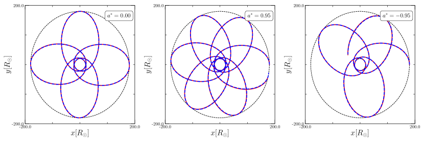
Figure 1: This figure shows the trajectories of a rigid body in Kerr space-time for various spin parameter values, as indicated in the legend. The center of mass of the rigid body, obtained from SPH simulations, is represented in red. Additionally, a dashed blue line depicts the trajectory for the test particle geodesic, obtained independently of SPH. In all SPH simulations, the center of mass is situated on the equatorial plane. The apocenter ($r_{a}$) and pericenter ($r_{p}$) remain constant across all simulations, with the outer black dotted circle denoting the apocenter.

To ensure correct implementation in the SPH code, we perform long-duration simulations of the orbital motion of a rigid body around a $10^{6}M_{\sun}$ Kerr BH in the equatorial plane, assuming a polytropic EOS for the rigid body. In these simulations, the pericenter distance is chosen such that it remains significantly greater than the tidal radius ($r_{t}$), ensuring that the star is not tidally interacting. We then verify that the stellar center of mass follows the point particle geodesic obtained independently of the SPH code with the same initial conditions for different $a^{\star}$ values, see Figure 1. This testing verifies the accuracy of the Kerr metric acceleration within our SPH code.

Next, to create a uniformly spinning star in a relaxed state, we follow the procedure outlined in García-Senz et al. (2020). Initially, we generate a relaxed fluid star in SPH without any rotation. The SPH particles are initially distributed in a close-packed sphere, and their radial positions are then adjusted to match the desired density profile. For polytropic models, the desired density profile is obtained by solving the Lane–Emden equation, while for WD models, it is achieved by solving the hydrostatic equilibrium equation and mass conservation equation simultaneously, as detailed in Garain & Sarkar (2023). The stretching of particle positions reduces statistical noise resulting from random particle placement. However, to settle the internal properties, such as density, the fluid star needs to evolve in isolation. The final relaxed fluid star is attained after evolution, ensuring its kinetic energy is within a specified tolerance level and its density profile converges to the desired configuration.

Once we obtain the relaxed fluid star without rotation, we introduce rigid rotation and allow the system to relax in the presence of internal dissipation, i.e., artificial viscosity. To eliminate velocity field noise and quickly reach equilibrium, we periodically set velocities to zero in the co-moving reference frame. During the initial relaxation, resetting occurs at shorter intervals, $dt=t_{sc}/3$ (where $t_{sc}$ is the sound crossing time), repeated five times consecutively. After that, the system is reset at longer intervals, $dt=0.8t_{sc}$, until the fluctuation in angular velocity is $0.1\%$ of the desired angular velocity for star rotation. Finally, we allow the system to evolve freely without resetting velocities for a sufficiently long period, ensuring oscillations around average values of star properties – central density, polar and equatorial radius, and total kinetic, internal, and gravitational energies – remain below $2.5\%$. This methodology has been validated as widely applicable to various stellar models, ranging from polytropic stars to WDs.

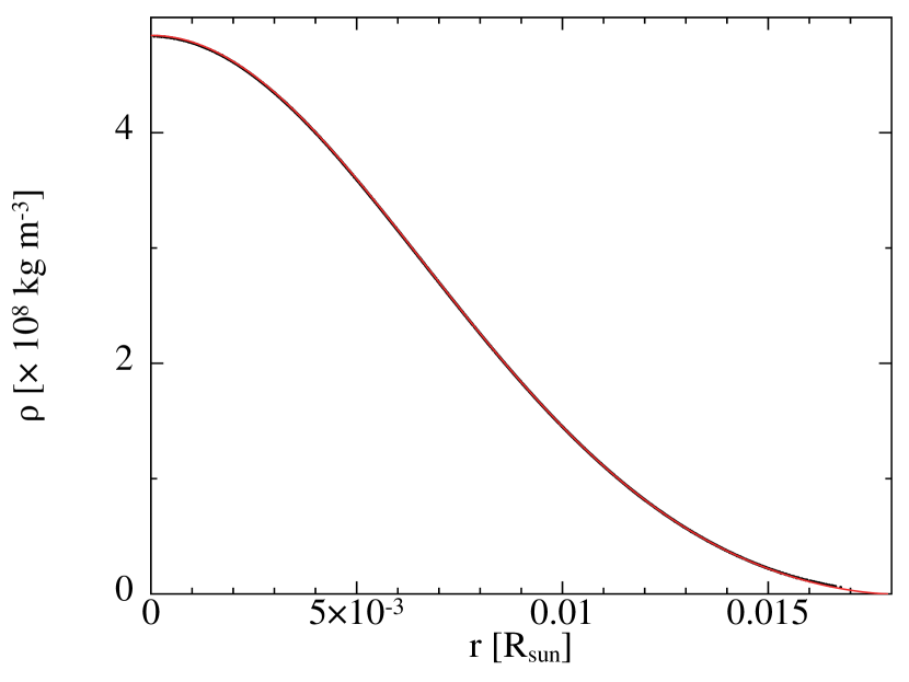
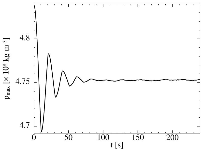
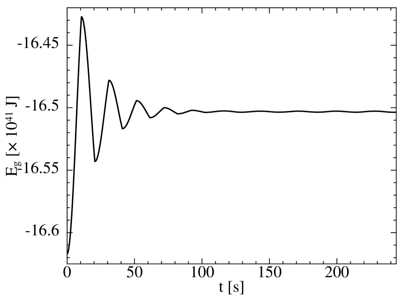
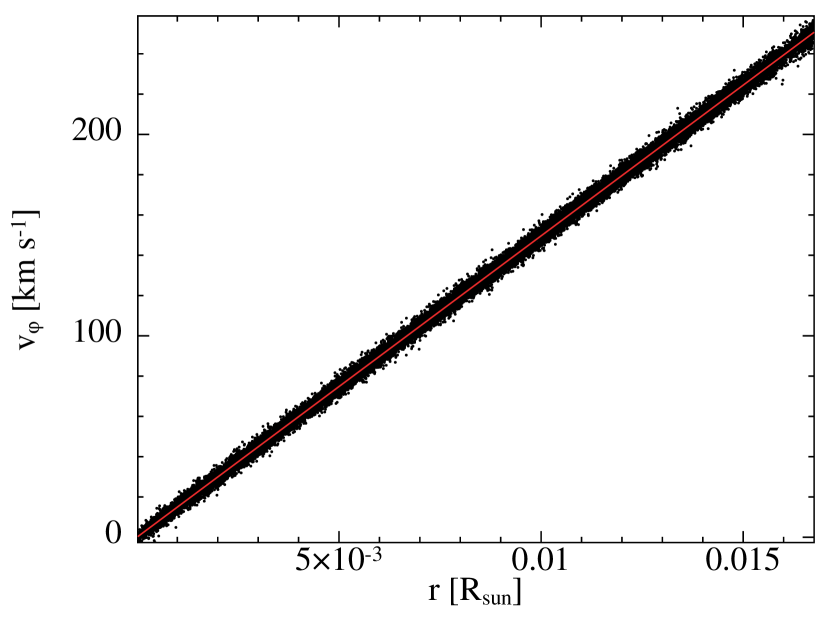
Figure 2: Top Left panel: The density is plotted against the radius for SPH particles using black dots for a relaxed, non-spinning WD of mass $0.3M_{\odot}$, with the theoretical solution depicted by the red line. Top Right panel: The maximum central density is depicted over time after imposing rigid rotation. Bottom Left panel: The total self-gravitational energy is plotted with time. Bottom Right panel: The azimuthal velocity for SPH particles (black dots) plotted against distance from the rotation axis, alongside the theoretical solution (red line) after relaxation. These figures are generated using SPLASH (Price, 2007).

The maximum spin that a star can sustain without breaking apart is determined by setting the self-gravitational force of the star equal to the centrifugal force. The angular velocity at which the star would break up is then calculated as $\Omega_{\rm br}=\sqrt{\frac{GM_{\star}}{R_{\star}^{3}}}$. Here, $M_{\star}$ and $R_{\star}$ represent the mass and radius of the star, respectively. If the star is spinning with an angular velocity $\Omega_{\star}$, the break-up fraction is defined as $\lambda=\Omega_{\star}/\Omega_{\rm br}$. We note that the above analysis is done assuming that the star is spherical, so that $\Omega_{\rm br}$ is the break-up angular speed at the stellar equator. If the star on the other hand is assumed to be spheroidal, then by using the Roche model, the maximum value of the break up angular speed can be calculated to be $\sim 0.54\Omega_{\rm br}$ (Shapiro & Teukolsky, 1983). In this paper, we will conservatively choose $\lambda=0.15$.

In Figure 2, we present the process of creating a relaxed, uniformly spinning WD with a mass of $0.3M_{\odot}$ and a radius of $0.018R_{\odot}$. In the Top Left panel, we show the density profile of the SPH particles after the initial relaxation from the stretch map, demonstrating a close match with the theoretical profile obtained independently of the SPH code. After achieving the relaxed profile for the non-spinning WD, we set up the WD in rigid rotation with an angular velocity of $\Omega_{\star}=\lambda\,\Omega_{\rm br}$, specifically choosing $\lambda=0.15$. Following a few velocity resets in the co-moving reference frame, we allow the spinning WD to evolve over a significant period, observing that fluctuations in its properties remain within acceptable tolerance levels. In particular, we show the variation of two properties, maximum central density $\rho_{\rm max}$ and total self-gravitational energy $E_{\rm g}$, as functions of time in the Top Right and Bottom Left panels of Figure 2, respectively. In the Bottom Right panel, we present the azimuthal velocities of the particles as a function of the distance from the rotational axis after the relaxation of the spinning WD, along with the exact solution ($v_{\phi}=\Omega_{\star}r$, where $r$ is the distance from the rotation axis). The close match between the numerical and theoretical solutions validates the correctness of our process for creating a uniformly spinning WD.

The rotation imposed on our WD corresponds to a rotational time-period of $\sim$ 5 minutes. This should be contrasted with the values obtained by Pelisoli et al. (2022) (24.93 seconds) and Kilic et al. (2021) (70 seconds) that we have mentioned in the introduction. Here, we consider the angular speed of the WD to be substantially less than the values reported in these works, which justifies to some extent our exclusion of magnetic field effects and we focus on obtaining the necessary features for TDEs that are dependent on stellar spin. The issue of TDEs involving spinning magnetic WDs is left for the future.

2.2 Simulation parameters

To simulate TDEs, we employ the SPH code developed by Banerjee et al. (2023) with the modifications mentioned above. The code uses a fast recursive binary tree to efficiently search neighboring particles and calculate particle accelerations. The tree accuracy parameter, which determines when a distinct node acts as a multipole source of gravity or is further bisected, is set to $\theta=0.5$. Standard artificial viscosity parameters, $\alpha^{\rm{AV}}=1.0$ and $\beta^{\rm{AV}}=2.0$, are used, and additionally, the Balsara switch is employed to reduce viscosity in shear flows (Balsara, 1995). The system evolves using a global time step, and SPH equations are integrated using the leapfrog integrator (K-D-K approach) to ensure conservation of mass, momentum, and energy.

To gain a comprehensive understanding of TDEs, works in the available literature have extensively explored their dependence on parameters such as $M$, $M_{\star}$, $R_{\star}$, the EOS of the star, eccentricity $e$ of the orbit, and impact parameter $\beta=r_{t}/r_{p}$. Some studies, such as those conducted by Tejeda et al. (2017), Gafton & Rosswog (2019), have examined the impact of BH spin on TDEs and debris properties. On the other hand, studies including Kagaya et al. (2019), Golightly et al. (2019b), Sacchi & Lodato (2019), have explored TDEs in the presence of stellar rotation. Notably, Golightly et al. (2019b) investigated the impact of stellar rotation on the fallback rate in the presence of a supermassive BH. However, to our knowledge, there has been no study examining TDEs by coupling BH spin with stellar rotation.

To focus on the essential effects arising from the coupling of BH-WD rotations while maintaining a manageable parameter space, we initially fix the orbit, specifying the eccentricity and $\beta$. We also include a spinning IMBH with a fixed mass and then set the mass, radius, and EOS for the WD. This narrows down the parameters of the system, leaving us with two independent variables corresponding to BH rotation and WD rotation. We will then study how these rotations impact the observables. We remind the reader that we opt for an IMBH with a mass of $M=10^{4}M_{\odot}$ and a WD of mass $M_{\rm wd}=0.3M_{\odot}$ and radius $R_{\rm wd}=0.018R_{\odot}$. To relate the pressure to the density of the WD’s fluid particles, we utilize a zero-temperature EOS, as described in Garain & Sarkar (2023). We generate relaxed WDs using the methodology discussed in the preceding subsection (Section 2.1), varying the break-up fraction ($\lambda$) with values of $0$, $0.05$, and $0.15$, where $\lambda=0$ corresponds to a non-spinning WD. For BH rotation, we choose specific spin parameters, $a^{\star}=0.98,0.0,-0.98$, with $a^{\star}=0$ corresponding to a Schwarzschild BH. Opting for higher values of the BH spin parameter aims to maximize rotational effects on observables. Subsequently, we consider an elliptical orbit with an eccentricity of $0.9$ and $r_{p}\simeq 39\,r_{g}$, where $r_{g}=GM/c^{2}$ represents the gravitational radius of the BH. This choice of $r_{p}$ ensures partial disruption. The presence of the surviving core modifies the late-time slope from the full disruption scenario Cufari et al. (2022). The center of mass for both the relaxed spinning and non-spinning WDs is positioned initially at a distance of $5r_{t}\simeq 136\,r_{g}$ from the BH in the equatorial plane, with the BH located at the origin.

We simulate a single interaction of the WDs with the IMBH, and after this interaction, the tidally disrupted material forms two tails along with the surviving core, returning to the pericenter due to the initial bound orbit. Simulations continue until all material bound to the BH is accreted. To manage computational costs, circularization and disk formation processes are omitted. The accretion radius is expanded from $2\,r_{g}$ to $3\,r_{t}\simeq 82\,r_{g}$ as the bound material returns to the IMBH. The mass falling back onto the accretion radius is tracked over time, and the numerical derivative of the data provides the fallback rate. The fallback rates are determined directly from simulations using methods outlined in Coughlin & Nixon (2015), Golightly et al. (2019a), Miles et al. (2020), Garain et al. (2023). Our simulations employ $5\times 10^{5}$ particles to model the relaxed WDs.

3 Results

In this section, we study the impact of rotation on the key observables of TDEs. All simulations start from identical initial positions of the WDs, and the pericenter distance $r_{p}$ is kept fixed. After the interaction, a self-gravitating core forms along with a bound and an unbound tail. To identify particles bound to the core, we use an energy-based iterative approach following Guillochon & Ramirez-Ruiz (2013). We look at the mass of the self-gravitating core, the fate of the bound debris, the rates at which material falls back, the spin of the core, and the emission of gravitational waves during the interaction. Before we explore how the rotations of both the BH and the WD together affect the entire process, we will first examine the effects of each rotation separately. This will help us get a clearer understanding of rotation of the BH, stellar rotation and their coupled effect influences the observables.

3.1 Fate of the Bound Debris and Fallback Rates

To determine the influence of BH rotation on the core and bound debris, we examine the tidal interaction between a non-spinning WD and a Kerr BH in elliptical trajectories. The core mass fraction, defined as the ratio of core mass over the initial mass, remains at $1.00$ until it reaches the pericenter. As a result of the WD’s partial disruption, the core mass fraction decreases over time, finally settling to a constant value. However, as depicted in Figure 3, Top Right panel, the core mass fraction exhibits variation with the BH spin parameter $a^{\star}$. Retrograde orbits ($a^{\star}<0$) experience more disruption compared to prograde orbits ($a^{\star}>0$). Here, the time is normalized with respect to the time to reach the pericenter. Similar effects have been observed by Kesden (2012) and Haas et al. (2012). For the same impact parameter, they found that stars are more easily disrupted in retrograde orbits. One possible reason for more disruption in a retrograde orbit could be the stronger rotation of the WD’s orbit caused by the frame-dragging effect. This extra rotation, over time, increases the likelihood of the WD getting closer to the BH than its prograde counterpart, hence allowing tidal forces to overcome the WD’s self-gravity to a greater extent. As a result, there is more disruption compared to the prograde orbit. The precession of the orbits of the core center of mass for different $a^{\star}$ values is shown in the Top Left panel of Figure 3. Additionally, we plot the geodesics of the point particle obtained independently of the SPH code with the same initial conditions. Based on Banerjee et al. (2023), the SPH core center-of-mass orbits deviate from the test particle geodesic when the mass ratio ($q=M/M_{\star}$) is smaller than $10^{3}$. For our case, the mass ratio is approximately $3.3\times 10^{4}$, explaining the lesser deviations in the trajectories in our work.

In the Bottom Left part of Figure 3, we illustrate how the mass of the bound debris changes over time, considering various values of $a^{\star}$. We observe that for a retrograde orbit, the mass of the bound debris is higher compared to a prograde orbit. Finally, the bound material returns to the BH and falls onto it through the accretion radius ($3\,r_{t}\simeq 82\,r_{g}$). By calculating the numerical derivative of the falling mass over time, we obtain the fallback rate, shown in the Bottom Right part of Figure 3 for different values of $a^{\star}$. Due to the precession of the orbit, the bound debris from retrograde orbits reaches the accretion radius more quickly than from prograde orbits. As more mass is disrupted in retrograde orbits, the maximum value of the fallback rate ($\dot{M}$) is also higher for retrograde orbits compared to prograde orbits. The peak $\dot{M}$ does not vary by more than $11\%$ as the spin changes from prograde to retrograde, and the time of peak occurrence varies by less than $1\%$ when transitioning from prograde to retrograde orbit. The late-time fallback rate for all $a^{\star}$ values is similar, making it challenging to distinguish the spin of the BH from the fallback rate plots.

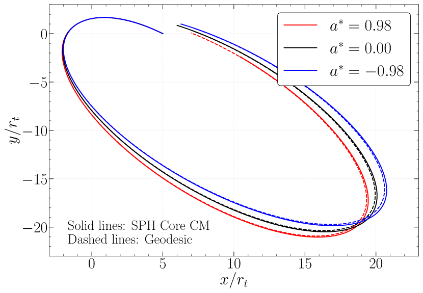
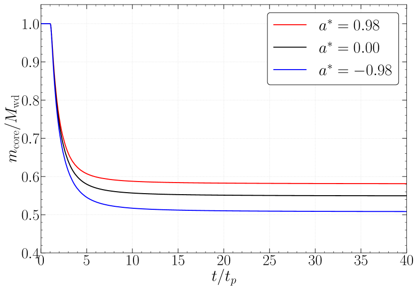
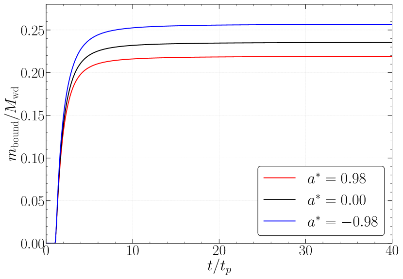
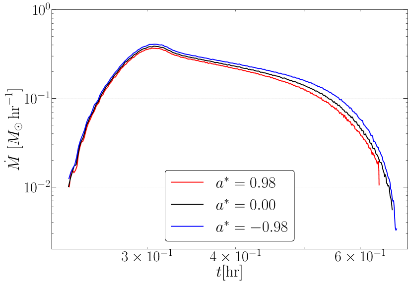
Figure 3: Top Left Panel: Trajectory of the center-of-mass of the core plotted (solid lines) along with the test particle geodesics (dashed lines). The $x$ and $y$ axes are normalized with respect to the tidal radius ($r_{t}$). Top Right Panel: Variation of the core mass fraction, $m_{\rm core}/M_{\rm wd}$, plotted against normalized time. Bottom Left Panel: Bound tail mass with respect to the initial WD mass varies with normalized time. Bottom Right Panel: Fallback rates plotted against time in hours. The different values of the BH spin parameter, $a^{\star}$, are mentioned in the legends.

Moving on, we study the impact of the initial uniform rotation of the WD on the bound debris and fallback rates in the presence of a non-spinning BH. With a maximum break-up fraction of $\lambda=0.15$ for the spinning WD, we find that the relative change in volume-equivalent radius between the spinning and non-spinning WDs, is approximately $0.5\%$, so that the impact parameter of the spinning and non-spinning WDs is almost the same. Consequently, the rotation of the initial WD significantly influences the dynamics of the disruption. The spinning WD, with initial rotation parallel (anti-parallel) to the orbital motion, is termed prograde (retrograde), where $\lambda>0$ ($\lambda<0$), and the orbital motion is along the positive $z$ direction.

As the WD gets closer to the BH, it undergoes radial stretching. When it reaches the position $r_{p}$, the tidal force exerts a torque on the WD, causing it to rotate to some extent. Consequently, after a partial disruption of the WD, the surviving core rotates with a non-zero rotational velocity in the direction of the orbital motion. In the case of prograde rotation, where the rotation after the tidal interaction aligns with the initial rotation, the rotation is enhanced. This leads to the disruption of more material and results in less mass for the surviving core compared to the initial non-spinning WD. In contrast, for retrograde spin of the WD, the initial rotation opposes the rotation after the tidal interaction, resulting in less mass being disrupted from the initial WD. The Left panel of Figure 4, illustrates the ratio of the surviving core mass to the initial WD mass over normalized time. We vary the break-up fraction from $-0.15$ to $0.15$ and observe different amounts of core mass from the initial WDs.

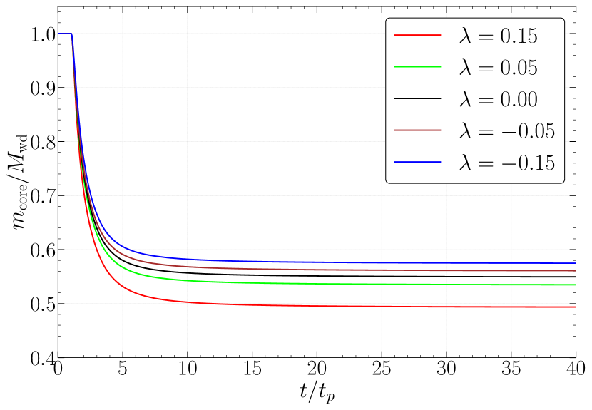
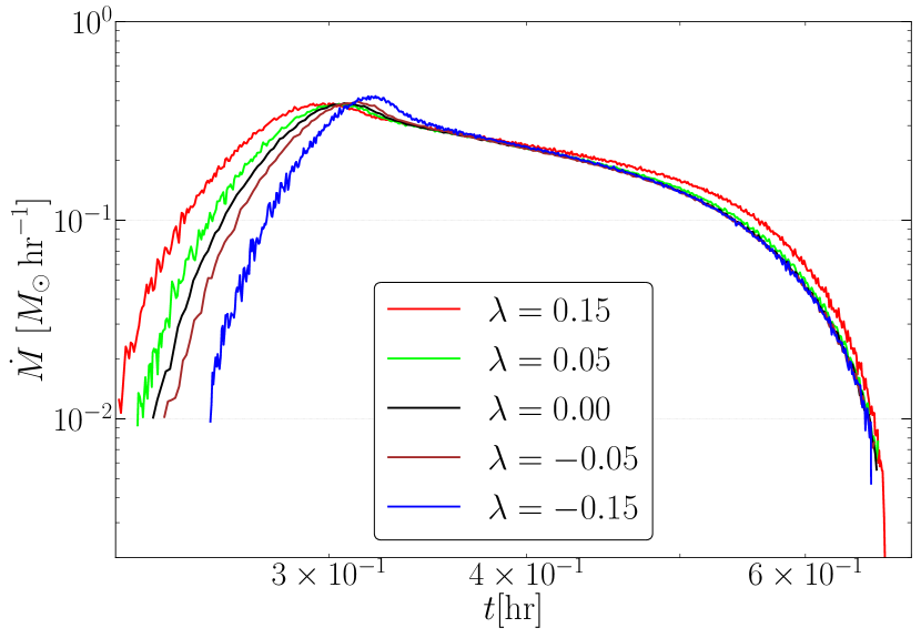
Figure 4: Left Panel: Variation of the core mass fraction, $m_{\rm core}/M_{\rm wd}$, plotted against normalized time. Right Panel: Fallback rates plotted against time in hours. The different values of the break-up fractions ($\lambda$) for different spinning WDs are mentioned in the legend.

Figure 5: We present the column density plots for the disrupted WDs after the interaction. All snapshots are taken at the same time, $t=0.08$ hours. The snapshots represent three different values of $\lambda$. It is observed that for prograde spin of the WD ($\lambda=0.15$), the debris is more distributed in the orbital plane, and the distribution gradually becomes more compact as we move from prograde spin to no spin to retrograde spin of the WD. These figures are generated using SPLASH.

In the Right panel of Figure 4, we show the fallback rate for different values of $\lambda$ over time in hours, considering a non-spinning IMBH. When the WD has a prograde spin, after disruption, the debris bound to the black hole is less compact compared to when the WD has a retrograde spin. In Figure 5, we depict the density distribution of the disrupted WDs at a specific time for various $\lambda$ values mentioned in the legend. It is evident that the debris distribution is more spread out in the $x-y$ plane for the prograde spin compared to the retrograde spin. Consequently, the most bound debris falls back onto the black hole more quickly in the prograde case, as it is more dispersed in space. The change in the most bound fallback time for prograde spin is approximately $14\%$ quicker than the retrograde spin of the WD. However, the late-time fallback is similar for all spinning WDs in the presence of a non-spinning BH. Consequently, inferring the properties of the BH spin (as argued before) and the initial spin of the WD from the late-time slope becomes difficult.

Next, we explore the combined rotation effects of the BH and WD on the material bound to the BH and the resulting fallback rates. In the presence of a spinning BH and a non-spinning WD, we observe that for retrograde spin ($a^{\star}<0$), there is more mass disruption from the initial WD compared to the prograde spin of the BH ($a^{\star}>0$). Conversely, in the presence of a non-spinning BH and a spinning WD, the prograde spin of the WD (parallel to the orbital direction, $\lambda>0$) leads to more disruption from the initial WD than the retrograde spin (anti-parallel to the orbital direction, $\lambda<0$) of the initial WD. Therefore, to achieve maximum disruption from the initial WD, coupling the retrograde spin of the BH with the prograde spin of the WD is required, while for minimum disruption, coupling the prograde spin of the BH with the retrograde spin of the WD is necessary. All other combinations fall between these chosen configurations.

In the Top Left panel of Figure 6, we display the variation in core mass fraction over normalized time. Notably, we observe a nearly $35\%$ relative change in core mass fraction from the minimum to the maximum disruption, contrasting with around $14\%$ for the scenario with a spinning BH and non-spinning WD, and approximately $16\%$ for a non-spinning BH and spinning WD. Hence, the “coupled” rotation significantly influences the disruption dynamics. The increased precession of the retrograde orbit of the BH, combined with the initial spin of the WD in the direction of the WD’s orbital motion, enhances the disruption from the initial WD. We also show the variation in bound tail mass and the mass difference between the two tidal tails ($\Delta m$) against normalized time in the Top Right and Bottom Left panels of Figure 6, where the masses are normalized with respect to the initial WD mass. Both bound tail mass and mass difference increase notably for the retrograde orbit of the BH coupled with the prograde spin of the WD. The presence of “coupled” rotation significantly influences the bound tail mass relative to the initial WD mass, with an approximately $40\%$ increase from minimum to maximum disruption. In contrast, for individual rotations with a spinning BH and spinning WD, the changes are approximately $17\%$ and $18\%$, respectively. We also observe a substantial change in the mass difference between the two tidal tails for “coupled” rotation, providing a kick velocity to the surviving core. However, the computed change in specific orbital energy of the surviving core relative to the initial specific orbital energy of the WD in the scenario with the maximum mass disruption is of the order of $10^{-5}$, as a result of which the disrupted WD does not leave the gravitational influence of the BH after the first interaction.

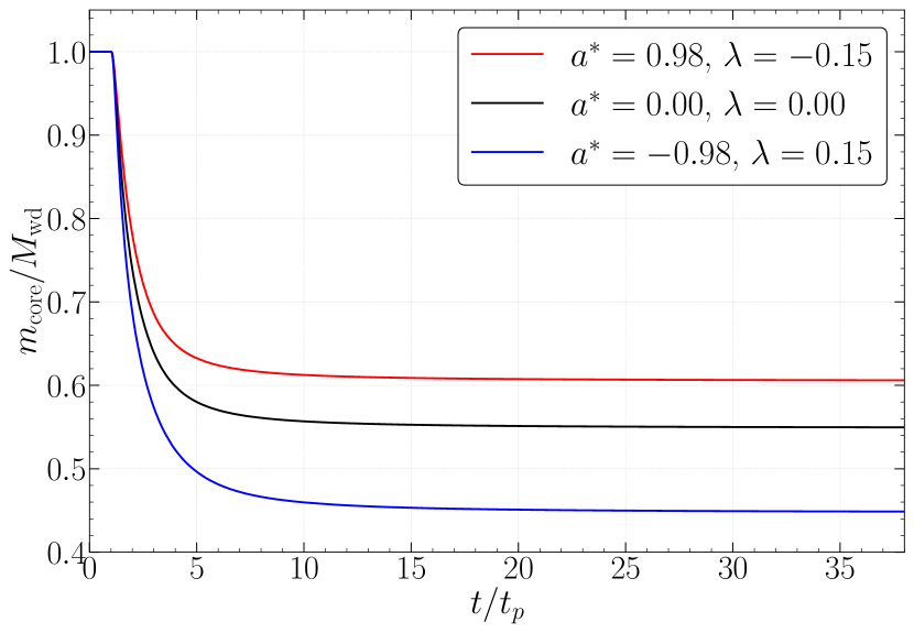
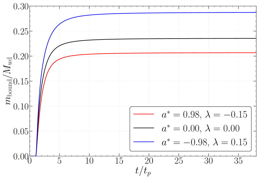
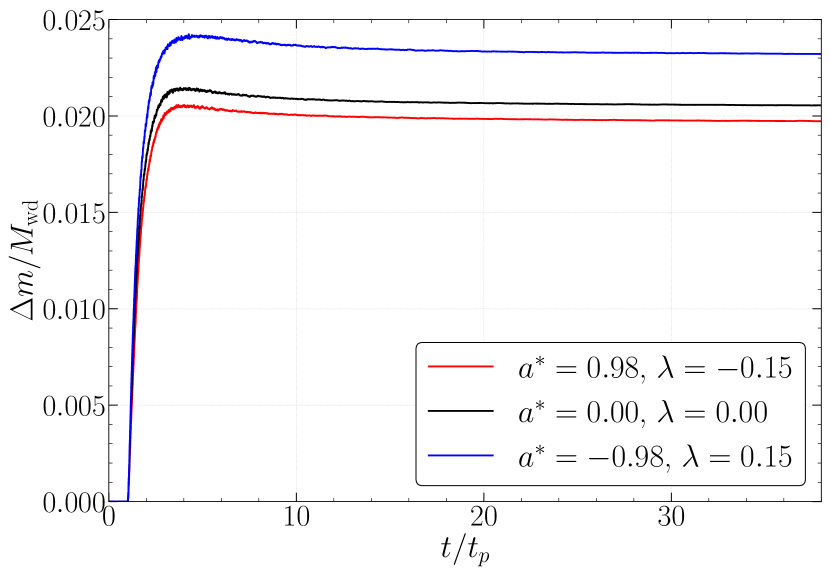
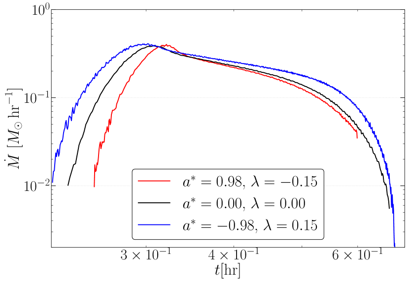
Figure 6: Top Left Panel: Core mass fraction variation, $m_{\rm core}/M_{\rm wd}$, plotted against normalized time. Top Right Panel: Bound tail mass relative to the initial WD mass varies with normalized time. Bottom Left Panel: Mass difference between the two tidal tails relative to the initial WD mass, plotted against normalized time. Bottom Right Panel: Fallback rates plotted against time in hours. Legends indicate the values of BH spin parameters ($a^{\star}$) and break-up fraction of the WDs ($\lambda$).

In the Bottom Right panel of Figure 6, we depict the fallback rates for three different combinations over time. The entire fallback process takes less than $1$ hour to complete for all cases. Notably, the most bound debris fallback time varies among different combinations, with a relative change of approximately $15\%$ from the coupling of prograde BH and retrograde WD to the coupling of retrograde BH and prograde WD. However, as previously discussed, the most bound debris fallback time is significantly influenced by the initial spin of the WD compared to the rotation of the BH. Hence, in the case of “coupled” rotation, the change in the most bound debris fallback rate time is mainly contributed by the spin of the WD. This change also affects the occurrence time of maximum $\dot{M}$. Nevertheless, we note that the maximum values of $\dot{M}$ do not vary significantly due to the rotation effects.

To conclude this subsection, we summarize that the disruption of the initial WD significantly varies with the “coupled” rotation effects of BH and WD. Observables such as core mass, bound tail mass, and the mass difference between the two tidal tails strongly depend on rotational effects. However, we find that, from the fallback rate plots, the most bound debris fallback time is highly dependent on the initial rotation of the WD and does not vary significantly with BH rotation. The late-time fallback characteristics are also very similar for all cases, making it difficult to determine stellar or BH rotations from the fallback rate plots.

3.2 Spin of the Surviving Core

We explore how tidal interaction affects the spin of the surviving core. As explained earlier, the tidal torque induces rotational motion in the disrupted WD after interacting with the BH. Therefore, it is interesting to understand how the initial prograde and retrograde rotations of the WD influence the spin of the surviving core while keeping the BH non-spinning. To calculate the spin of the surviving core, we compute the spin angular momentum of particles bound to the core using the formula $\mathbf{L}=\sum_{i}m_{i}(\mathbf{r}_{i}\times\mathbf{v}_{i})$, where the index $i$ runs over all bound particles, and $r_{i}$ and $v_{i}$ are calculated relative to the center of mass of the core. Since the orbital motion of the center of mass is in the $x-y$ plane, the relevant direction for the spin angular momentum is the $z$-direction.

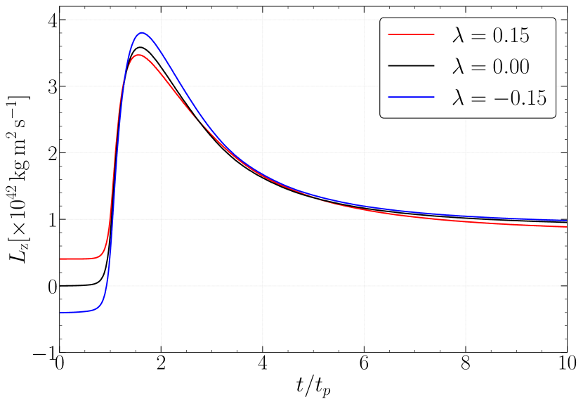
Figure 7: Variation of the $z$-component of the spin angular momentum with time for bound particles. The entire WD is bound before reaching $r_{p}$, and after interaction, the bound core maintains a saturation value of $L_{z}$. The initial rotation of the WD induces a change in the initial $L_{z}$ values, as indicated in the legend for different spinning WDs.

In Figure 7, we show the variation in the $z$-component of the spin angular momentum $L_{z}$ as a function of the normalized time, considering three values of $\lambda$ to understand the effects of the initial spin. In all cases ($\lambda=0,\pm 0,15$), we find that the tidal torque increases $L_{z}$, with the maximum change resulting in the case of retrograde stellar rotation, that has its angular momentum reversed due to the tidal torque. Note that the peak value of $L_{z}$ is greater in this case than the others due to the fact that the number of particles in the bound core is greater here, although the saturation values of the angular momentum is almost the same as the other cases. The rotation induced in the surviving core could alter the disruption dynamics in subsequent interactions with the BH, which could be an interesting topic for future study. We also mention that there is no significant change in the spin angular momentum profile in the case of the non-spinning WD and spinning BH configuration. When both the BH and the WD spins, we find that the profiles are predominantly influenced by the initial spin of the WD and are qualitatively similar to Figure 7.

From Figure 7, we also note that after the first pericenter passage, the angular momenta of both pro and retrograde spinning stars are almost identical to the non-spinning one. Hence the information about the initial stellar spin is lost after this first passage and initial stellar spin will not substantially change conclusions on multiple pericenter passages. Such a situation involving IMBHs and main sequence stars have recently been reported in Kıroglu et al. (2023).

3.3 Gravitational Wave Emission

Once the WD nears $r_{p}$ and interacts with the BH, it emits strong gravitational waves (GWs). Following the disruption, the stretched debris is less compact to emit robust gravitational waves after leaving the closest approach. As a result, the detectable gravitational wave signal exhibits a burst-like behavior. The GW amplitudes, $h_{+}$ and $h_{\times}$, for an observer along the $z$-axis at a distance $d$ are calculated using the formulas of Rosswog et al. (2009):

$$h_{+}=\frac{G}{c^{4}d}\left(\ddot{I}_{xx}-\ddot{I}_{yy}\right)~{},~{}~{}h_{\times}=\frac{2G}{c^{4}d}\ddot{I}_{xy}~{}.$$ (5)

Here, $\ddot{I}_{ij}$ represents the second-time derivative of the reduced quadrupole moment $I_{ij}$ (Centrella & McMillan, 1993)

$${I}_{ij} =\sum\limits_{a=1}^{N}m_{a}\left(x_{ia}x_{ja}-\frac{1}{3}\delta_{ij}r_{a}^{2}\right)~{},$$ (6)

where $m_{a}$ is the mass of the $a$th particle, and the index $a$ runs over all particles.

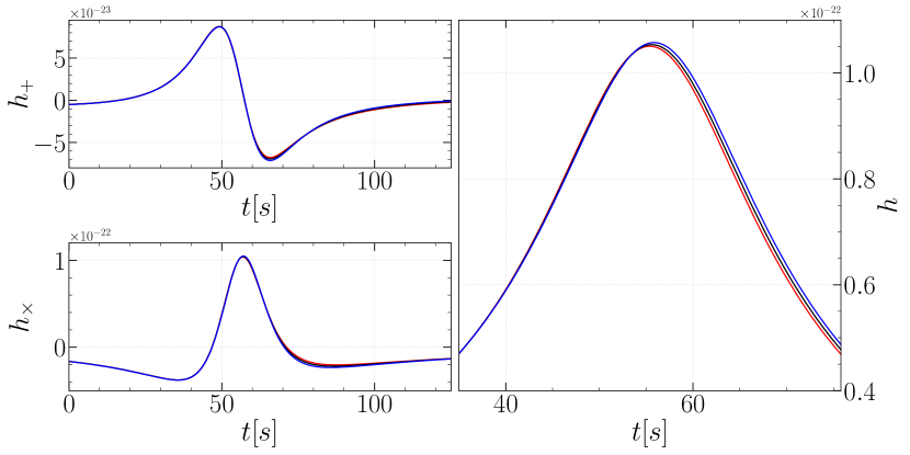
Figure 8: GW emission resulting from the tidal interaction between a WD with a mass of $0.3M_{\odot}$ and an IMBH with a mass of $10^{4}M_{\odot}$. The source is located at a distance of $20$ Mpc. Top Left Panel: Variation of $\times$ polarization with time in seconds. Bottom Left Panel: Variation of + polarization with time in seconds. Right Panel: Variation of the root-square-sum amplitude with time in seconds. Different curves correspond to various values of $a^{\star}$ and $\lambda$ as indicated in the legend.

We studied variations in the amplitude of $h_{+}(t)$, $h_{\times}(t)$, and the root-square-sum amplitude, $\lvert h(t)\rvert=\sqrt{\lvert h_{+}(t)\rvert^{2}+\lvert h_{\times}(t)\rvert^{2}}$ over time for different tidal disruption scenarios. Figure 8 displays the GW strains for three specific scenarios mentioned in the legend. For non-spinning BH with spinning WD tidal disruption scenarios, all GW strains are similar and do not deviate from each other, following the black lines in Figure 8. Therefore, we choose not to display them, concluding that distinguishing initial spin of the WDs from GW strains is challenging. To substantiate this last point, we ran three further simulations with $r_{p}=15r_{g}$ where it may still be reasonable to treat the stellar hydrodynamics in the Newtonian limit (Stone et al., 2019). We found that spinning and non-spinning WDs produced identical GW strains even for this case.

In Figure 8, we show the combinations resulting in maximum and minimum disruptions for presentation. We observe that the polarization amplitudes depend on the spin of the BH. As we increase the BH spin from retrograde to prograde, the peak of the root-sum-square amplitude $h$ shifts to earlier times and decreases. The relative change in the peak of $h$ from prograde to retrograde is approximately $0.7\%$. It is worth mentioning that Toscani et al. (2022) also observed a similar behavior of the root-sum-square amplitude with BH spin, noting a significant variation in the peak value of $h$ for their chosen parameters as they consider higher $\beta$ values for tidal interaction.

4 Discussions and conclusions

To conclude this paper, let us first tie up a few loose ends that we left in section 2. First, we note that as mentioned in the beginning of section 2, we have treated the hydrodynamics of the star in a Newtonian manner. This approximation can be justified if two conditions are satisfied. (a) The stellar gravity is close to Newtonian and (b) the external gravity (that due to the BH) varies slowly over scales comparable to the diameter of the star. Both these conditions are satisfied for the IMBH-WD system that we consider. As for point (a), recall that a useful measure to glean whether a Newtonian treatment of stellar gravity is consistent is given by the surface redshift factor $z$, defined via $z+1=(1-2GM_{\star}/c^{2}R_{\star})^{-1/2}$. Now, for the WD that we have considered, $z\simeq 3.5\times 10^{-5}$, which is small enough to indicate that the star is effectively Newtonian (compare this for example with $z\simeq 2\times 10^{-6}$ for the Sun and $z\sim 0.2$ for a typical $1.4M_{\odot}$ neutron star with a radius of 10 Km). To see if point (b) is satisfied here, we note that one often defines a local radius of curvature ${\mathcal{R}}\sim(r^{3}c^{2}/GM)^{1/2}$ to estimate the effect of gravity over a given length scale (Taylor & Poisson, 2008; Poisson & Vlasov, 2010; Tejeda et al., 2017). In our case, at $r_{p}=39r_{g}$ where this radius of curvature is minimum, we find ${\mathcal{R}}/R_{\star}\sim 277$ indicating that the effects of BH gravity is indeed a constant to a good approximation over the dimension of the star. Indeed, for closer encounters with smaller values of $r_{p}$, this ratio becomes smaller, and the treatment of the stellar fluid using Newtonian hydrodynamics is more challenged. In that situation, one should possibly write the fluid equations in terms of the Boyer-Lindquist coordinates as done by Tejeda et al. (2017), which we have not done here.

The second assumption that we have made is regarding the geodesic nature of the spinning particles that we have considered here (see the discussion after Equation 3). Now, the deviation from geodesic trajectories of spinning particles can be estimated by converting the specific angular momentum of the star to a length scale (upon dividing by $c$) and comparing it with the BH mass on the same scale (upon multiplying by $G/c^{2}$), see Semerak (1999). The smallness of the ratio of the specific angular momentum to the BH mass on the same length scale is an indicator of deviation from geodesic behaviour. In our case, we numerically computed this ratio at the initial stellar position of $5r_{t}$ and at $r_{p}$, and found this to be $1.5\times 10^{-4}$ and $1.3\times 10^{-3}$, respectively. This indicates that geodesics are a good approximation in the context of the spinning WD that we have considered, see the discussion in Semerak (1999).

Now we summarise our main results. In this paper we have considered partial tidal disruptions of spinning WDs in the background of spinning IMBHs. We have shown that the “coupling” between stellar and BH spins might considerably alter the physics of the process. In the most extreme cases exemplified in Figure 6, the core mass fraction and the bound tail mass might change by as much as $\sim 40\%$ compared to the case when one considers only stellar or black hole spin. We have also shown the time at which peak fallback occurs is also a strong function of the coupling between the two spins, although the value of the maximum fallback rate does not seem to significantly depend on rotational effects. This last point, along with the fact that the late time fallback rate of debris does not significantly depend on rotational effects indicates that these quantities cannot possibly used to determine stellar or BH spin rates.

However, it is important to highlight the potential observational significance of our study in understanding hypervelocity stars (HVSs). HVSs are stars presumed to possess velocities surpassing the escape velocity of its Galaxy. Theoretical proposals by Hills (1988) suggest that such high-velocity stars could result from the tidal interaction of a stellar binary with a supermassive black hole, attaining velocities more than $1000\,\rm{km\,s^{-1}}$. Additionally, HVSs may originate from interactions involving single stars and an IMBH (Yu & Tremaine, 2003) or scattering off stellar-mass black holes segregated in the Galactic Center (O’Leary & Loeb, 2008). Observationally, the discovery of the first HVS with a radial velocity of $709\,\rm{km\,s^{-1}}$ in the Galactic rest frame was reported by Brown et al. (2005). Subsequently, a large HVSs have been identified, with a comprehensive review available in Brown (2015). A recent discovery of HVS, S5-HVS1, with a total velocity of $1755\pm 50\,\rm{km\,s^{-1}}$, was reported by Koposov et al. (2020).

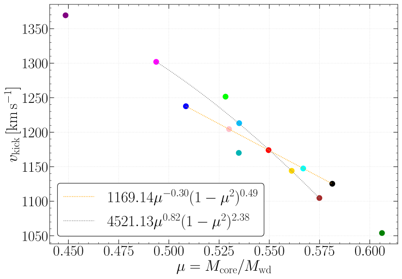
Figure 9: We show the kick velocity ($v_{\rm kick}$) of the surviving core as a function of the core mass fraction ($M_{\rm core}/M_{\rm wd}$). The two well-fitted equations in the legend correspond to the following scenarios: the first (orange dotted) involves a spinning BH and a non-spinning WD, while the second (gray dotted) involves a non-spinning BH and a spinning WD. In the case where both the BH and the WD spin, no simple fitting of the data values is found.

Our study on the tidal disruption of WDs due to IMBHs introduces a plausible explanation for the origins of these high-velocity stars. In the partial disruption scenario, the outer layers of the WD are ejected, leaving behind a self-bound core. The asymmetric tidal tails formed during this process may impart a specific orbital energy, resulting in a velocity ‘kick’ to the core. The kick velocity of the self-bound core is calculated using the formulation by Manukian et al. (2013), given by $v_{\rm kick}=\sqrt{2(\epsilon-\epsilon_{0})}$, where $\epsilon$ is the final specific orbital energy of the saturated core, and $\epsilon_{0}$ is the initial specific orbital energy of the WD.

In Figure 9, we show the variations in kick velocity with respect to the core mass fraction. For spinning BH and non-spinning WDs, the kick velocity changes by approximately $10\%$ as the BH spin parameter, $a^{\star}$, varies from $0.98$ to $-0.98$, as shown by the orange dotted line. In contrast, tidal interaction between a non-spinning BH and spinning WDs results in an $18\%$ variation in kick velocities as the break-up fraction changes from $-0.15$ to $0.15$, represented by the gray dotted line. However, in the case where both the BH and the WD spin, no such simple fitting is possible for these points. Although, the kick velocity for “coupled” rotation ranges from a maximum of $1370\,\rm{km\,s^{-1}}$ to a minimum of $1054\,\rm{km\,s^{-1}}$, corresponding to maximum and minimum disruption scenarios, with an approximate change of $30\%$. As the kick velocity of the core increases, it ultimately enhances the eccentricity of the core’s orbit. Multiple such interactions with the BH will enhance the specific orbital energy of the core, leading to its ejection from the influence of the BH and transforming into a HVS. This highlights the significant impact of BH and stellar spins in determining kick velocities, potentially contributing to the understanding of the high velocities observed in HVSs. Further observational and theoretical studies can provide valuable insights into these intriguing astrophysical phenomena.

Acknowledgements

We acknowledge the support and resources provided by PARAM Sanganak under the National Supercomputing Mission, Government of India, at the Indian Institute of Technology Kanpur. We thank Pritam Banerjee for very useful comments and discussions. The work of DG is supported by grant number 09/092(1025)/2019-EMR-I from the Council of Scientific and Industrial Research (CSIR). The work of TS is supported in part by the USV Chair Professor position at IIT Kanpur, India.

Data Availability Statement

The data underlying this article will be shared upon reasonable request to the corresponding author.

References

- Abbott et al. (2020) Abbott, R., Abbott, T. D., Abraham, S., et al. 2020, Phys. Rev. Lett., 125, 101102. doi:10.1103/PhysRevLett.125.101102
- Balsara (1995) Balsara, D. S. 1995, Journal of Computational Physics, 121, 357. doi:10.1016/S0021-9991(95)90221-X
- Banerjee et al. (2023) Banerjee, P., Garain, D., Chowdhury, S., et al. 2023, MNRAS, 522, 4332. doi:10.1093/mnras/stad1284
- Bonnerot et al. (2016) Bonnerot, C., Rossi, E. M., Lodato, G., et al. 2016, MNRAS, 455, 2253. doi:10.1093/mnras/stv2411
- Boshkayev et al. (2013) Boshkayev, K., Rueda, J. A., Ruffini, R., Siutsou, I., 2013, ApJ, 762, 117. doi:10.1088/0004-637X/762/2/117
- Brown (2015) Brown, W. R. 2015, ARA&A, 53, 15. doi:10.1146/annurev-astro-082214-122230
- Brown et al. (2005) Brown, W. R., Geller, M. J., Kenyon, S. J., et al. 2005, ApJ, 622, L33. doi:10.1086/429378
- Brown et al. (2015) Brown, G. C., Levan, A. J., Stanway, E. R., et al. 2015, MNRAS, 452, 4297. doi:10.1093/mnras/stv1520
- Cao et al. (2023) Cao, Z., Jonker, P. G., Wen, S., et al. 2023, MNRAS, 519, 2375. doi:10.1093/mnras/stac3539
- Carter & Luminet (1982) Carter, B. & Luminet, J. P. 1982, Nature, 296, 211. doi:10.1038/296211a0
- Carter & Luminet (1983) Carter, B. & Luminet, J.-P. 1983, A&A, 121, 97
- Centrella & McMillan (1993) Centrella, J. M. & McMillan, S. L. W. 1993, ApJ, 416, 719. doi:10.1086/173272
- Chen & Shen (2018) Chen, J.-H. & Shen, R.-F. 2018, ApJ, 867, 20. doi:10.3847/1538-4357/aadfda
- Chen et al. (2023) Chen, J.-H. Shen, R.-F. & Liu S-F., ApJ, 947, 32. doi:10.3847/1538-4357/acbfb6
- Chilingarian et al. (2018) Chilingarian, I. V., Katkov, I. Y., Zolotukhin, I. Y., et al. 2018, ApJ, 863, 1. doi:10.3847/1538-4357/aad184
- Claire et al. (2023) Claire S. Y, Fragione, G., Perna, R., 2023, ApJ, 953, 141. doi:10.3847/1538-4357/ace1eb
- Clerici & Gomboc (2020) Clerici, A. & Gomboc, A. 2020, A&A, 642, A111. doi:10.1051/0004-6361/202037641
- Coughlin & Nixon (2015) Coughlin, E. R. & Nixon, C. 2015, ApJ, 808, L11. doi:10.1088/2041-8205/808/1/L11.
- Coughlin et al. (2016a) Coughlin, E. R., Nixon, C., Begelman, M. C., et al. 2016a, MNRAS, 455, 3612. doi:10.1093/mnras/stv2511
- Coughlin et al. (2016b) Coughlin, E. R., Nixon, C., Begelman, M. C., et al. 2016b, MNRAS, 459, 3089. doi:10.1093/mnras/stw770
- Coughlin & Nixon (2019) Coughlin, E. R. & Nixon, C. J. 2019, ApJ, 883, L17. doi:10.3847/2041-8213/ab412d
- Cufari et al. (2022) Cufari, M., Coughlin, E. R., & Nixon, C. J. 2022, ApJ, 924, 34. doi:10.3847/1538-4357/ac32be
- Darbha et al. (2019) Darbha, S., Coughlin, E. R., Kasen, D., et al. 2019, MNRAS, 488, 5267. doi:10.1093/mnras/stz1923
- de Oliveira et al. (2020) de Oliveira, R. L., Bruch, A., Rodrigues, C. V., et al. 2020, ApJ, 898, L40. doi:10.3847/2041-8213/aba618
- Evans & Kochanek (1989) Evans, C. R. & Kochanek, C. S. 1989, ApJ, 346, L13. doi:10.1086/185567
- Frank & Rees (1976) Frank, J. & Rees, M. J. 1976, MNRAS, 176, 633. doi:10.1093/mnras/176.3.633
- Gafton et al. (2015) Gafton, E., Tejeda, E., Guillochon, J., et al. 2015, MNRAS, 449, 771. doi:10.1093/mnras/stv350
- Gafton & Rosswog (2019) Gafton, E. & Rosswog, S. 2019, MNRAS, 487, 4790. doi:10.1093/mnras/stz1530
- Garain et al. (2023) Garain, D., Banerjee, P., Chowdhury, S., et al. 2023, J. Cosmology Astropart. Phys, 2023, 062. doi:10.1088/1475-7516/2023/11/062
- Garain & Sarkar (2023) Garain, D. & Sarkar, T. 2023, arXiv:2310.03539. doi:10.48550/arXiv.2310.03539
- García-Senz et al. (2020) García-Senz, D., Cabezón, R. M., Blanco-Iglesias, J. M., et al. 2020, A&A, 637, A61. doi:10.1051/0004-6361/201936837
- Golightly et al. (2019a) Golightly, E. C. A., Nixon, C. J., & Coughlin, E. R. 2019a, ApJ, 882, L26. doi:10.3847/2041-8213/ab380d
- Golightly et al. (2019b) Golightly, E. C. A., Coughlin, E. R., & Nixon, C. J. 2019b, ApJ, 872, 163. doi:10.3847/1538-4357/aafd2f
- Greene et al. (2020) Greene, J. E., Strader, J., & Ho, L. C. 2020, ARA&A, 58, 257. doi:10.1146/annurev-astro-032620-021835
- Guillochon & Ramirez-Ruiz (2013) Guillochon, J. & Ramirez-Ruiz, E. 2013, ApJ, 767, 25. doi:10.1088/0004-637X/767/1/25
- Guillochon et al. (2014) Guillochon, J., Manukian, H., & Ramirez-Ruiz, E. 2014, ApJ, 783, 23. doi:10.1088/0004-637X/783/1/23
- Haas et al. (2012) Haas, R., Shcherbakov, R. V., Bode, T., et al. 2012, ApJ, 749, 117. doi:10.1088/0004-637X/749/2/117
- Hayasaki et al. (2013) Hayasaki, K., Stone, N., & Loeb, A. 2013, MNRAS, 434, 909. doi:10.1093/mnras/stt871
- Hayasaki et al. (2016) Hayasaki, K., Stone, N., & Loeb, A. 2016, MNRAS, 461, 3760. doi:10.1093/mnras/stw1387
- Hermes et al. (2017) Hermes, J. J., Gansicke B. T., Kawaler, S. D., et al., 2017 ApJS, 232, 23. doi:10.3847/1538-4365/aa8bb5
- Hills (1975) Hills, J. G. 1975, Nature, 254, 295. doi:10.1038/254295a0
- Hills (1988) Hills, J. G. 1988, Nature, 331, 687. doi:10.1038/331687a0
- Holoien et al. (2019) Holoien, T. W.-S., Vallely, P. J., Auchettl, K., et al. 2019, ApJ, 883, 111. doi:10.3847/1538-4357/ab3c66
- Jonker et al. (2022) Jonker, P. G, Arcavi, I., Phinney, E. S, et al. 2022, The Tidal Disruption of Stars by Massive Black Holes (Springer)
- Kagaya et al. (2019) Kagaya, K., Yoshida, S., & Tanikawa, A. 2019, arXiv:1901.05644. doi:10.48550/arXiv.1901.05644
- Kawaler (2003) Kawaler, S. D., 2003, in “Stellar Rotation,” Proc. IAU Symposium No. 215, eds. Maeder, A & Eenens, P.
- Kesden (2012) Kesden, M. 2012, Phys. Rev. D, 86, 064026. doi:10.1103/PhysRevD.86.064026
- Kilic et al. (2021) Kilic, M., Kosakowski, A., Moss, A. G., et al. 2021, ApJ, 923, L6. doi:10.3847/2041-8213/ac3b60
- Kıroglu et al. (2023) Kıroglu, F., Lombardi, J. C., Kremer, K., et al. 2023 ApJ948, 89. doi:10.3847/1538-4357/acc24c
- Kızıltan et al. (2017) Kızıltan, B., Baumgardt, H., & Loeb, A. 2017, Nature, 542, 203. doi:10.1038/nature21361
- Kochanek (1994) Kochanek, C. S. 1994, ApJ, 422, 508. doi:10.1086/173745
- Koposov et al. (2020) Koposov, S. E., Boubert, D., Li, T. S., et al. 2020, MNRAS, 491, 2465. doi:10.1093/mnras/stz3081
- Lacy et al. (1982) Lacy, J. H., Townes, C. H., & Hollenbach, D. J. 1982, ApJ, 262, 120. doi:10.1086/160402
- Law-Smith et al. (2017) Law-Smith, J., MacLeod, M., Guillochon, J., et al. 2017, ApJ, 841, 132. doi:10.3847/1538-4357/aa6ffb
- Law-Smith et al. (2019) Law-Smith, J., Guillochon, J., & Ramirez-Ruiz, E. 2019, ApJ, 882, L25. doi:10.3847/2041-8213/ab379a
- Law-Smith et al. (2020) Law-Smith, J. A. P., Coulter, D. A., Guillochon, J., et al. 2020, ApJ, 905, 141. doi:10.3847/1538-4357/abc489
- Lin et al. (2020) Lin, D., Strader, J., Romanowsky, A. J., et al. 2020, ApJ, 892, L25. doi:10.3847/2041-8213/ab745b
- Liptai et al. (2019) Liptai, D., Price, D. J., Mandel, I., et al. 2019, arXiv:1910.10154. doi:10.48550/arXiv.1910.10154
- Lodato et al. (2009) Lodato, G., King, A. R., & Pringle, J. E. 2009, MNRAS, 392, 332. doi:10.1111/j.1365-2966.2008.14049.x
- MacLeod et al. (2013) MacLeod, M., Ramirez-Ruiz, E., Grady, S., et al. 2013, ApJ, 777, 133. doi:10.1088/0004-637X/777/2/133
- Mainetti et al. (2017) Mainetti, D., Lupi, A., Campana, S., et al. 2017, A&A, 600, A124. doi:10.1051/0004-6361/201630092
- Manukian et al. (2013) Manukian, H., Guillochon, J., Ramirez-Ruiz, E., et al. 2013, ApJ, 771, L28. doi:10.1088/2041-8205/771/2/L28
- Matthison (1937) Mathisson, M., 1937, Acta Phys. Polon. 6, 167.
- Miles et al. (2020) Miles, P. R., Coughlin, E. R., & Nixon, C. J. 2020, ApJ, 899, 36. doi:10.3847/1538-4357/ab9c9f
- Misner et al. (1973) Misner, C. W., Thorne, K. S., & Wheeler, J. A. 1973, Gravitation, ISBN 0-7167-0334-3, ISBN 0-7167-0344-0 (pbk). San Francisco: W.H. Freeman and Company, 1973
- Nixon et al. (2021) Nixon, C. J., Coughlin, E. R., & Miles, P. R. 2021, ApJ, 922, 168. doi:10.3847/1538-4357/ac1bb8
- O’Leary & Loeb (2008) O’Leary, R. M. & Loeb, A. 2008, MNRAS, 383, 86. doi:10.1111/j.1365-2966.2007.12531.x
- Papapetrou (1951) Papapetrou, A., 1951 Proc. R. Soc. Lond. 209, 248.
- Park & Hayasaki (2020) Park, G. & Hayasaki, K. 2020, ApJ, 900, 3. doi:10.3847/1538-4357/ab9ebb
- Pelisoli et al. (2022) Pelisoli, I., Marsh, T. R., Dhillon, V. S., et al. 2022, MNRAS, 509, L31. doi:10.1093/mnrasl/slab116
- Phinney (1989) Phinney, E. S. 1989, The Center of the Galaxy, 136, 543
- Poisson & Vlasov (2010) Poisson, E., & Vlasov, I., 2010, Phys. Rev. D, 81, 024029. doi:10.1103/PhysRevD.81.024029
- Price (2007) Price, D. J. 2007, PASA, 24, 159. doi:10.1071/AS07022
- Rosswog et al. (2009) Rosswog, S., Ramirez-Ruiz, E., & Hix, W. R. 2009, ApJ, 695, 404. doi:10.1088/0004-637X/695/1/404
- Rees (1988) Rees, M. J. 1988, Nature, 333, 523. doi:10.1038/333523a0 .
- Ryu et al. (2020a) Ryu, T., Krolik, J., Piran, T., et al. 2020a, ApJ, 904, 98. doi:10.3847/1538-4357/abb3cf
- Ryu et al. (2020b) Ryu, T., Krolik, J., Piran, T., et al. 2020b, ApJ, 904, 100. doi:10.3847/1538-4357/abb3ce
- Ryu et al. (2020c) Ryu, T., Krolik, J., Piran, T., et al. 2020c, ApJ, 904, 100. doi:10.3847/1538-4357/abb3ce
- Sacchi & Lodato (2019) Sacchi, A. & Lodato, G. 2019, MNRAS, 486, 1833. doi:10.1093/mnras/stz981
- Semerak (1999) Semerak, O., 1999, MNRAS308, 863. doi:10.1046/j.1365-8711.1999.02754.x
- Shapiro & Teukolsky (1983) Shapiro, S. L., & Teukolsky, S. A., Black Holes, White Dwarfs and Neutron Stars, The Physics of Compact Objects, 1983, John Wiley & Sons, Inc.
- Stone et al. (2019) Stone, N. C., Kesden, M., Cheng, R. M., et al. 2019 Gen. Rel. Grav. 51, 30. doi:10.1007/s10714-019-2510-9
- Taylor & Poisson (2008) Taylor, S., & Poisson, E., 2008, Phys. Rev. D78, 084016. doi:10.1103/PhysRevD.78.084016
- Takekawa et al. (2019) Takekawa, S., Oka, T., Iwata, Y., et al. 2019, ApJ, 871, L1. doi:10.3847/2041-8213/aafb07
- Tejeda et al. (2017) Tejeda, E., Gafton, E., Rosswog, S., et al. 2017, MNRAS, 469, 4483. doi:10.1093/mnras/stx1089
- Tejeda & Rosswog (2013) Tejeda, E. & Rosswog, S. 2013, MNRAS, 433, 1930. doi:10.1093/mnras/stt853
- Toscani et al. (2022) Toscani, M., Lodato, G., Price, D. J., et al. 2022, MNRAS, 510, 992. doi:10.1093/mnras/stab3384
- Open TDE Catalog (2023) The Open TDE Catalog, 2023, available at https://tde.space/
- Ulmer (1999) Ulmer, A. 1999, ApJ, 514, 180. doi:10.1086/306909.
- Volonteri (2012) Volonteri, M. 2012, Science, 337, 544. doi:10.1126/science.1220843
- Wang et al. (2021) Wang, Y.-H., Perna, R., & Armitage, P. J. 2021, MNRAS, 503, 6005. doi:10.1093/mnras/stab802.
- Yu & Tremaine (2003) Yu, Q. & Tremaine, S. 2003, ApJ, 599, 1129. doi:10.1086/379546