LADDER: Revisiting the Cosmic Distance Ladder with Deep Learning Approaches and Exploring its Applications

Abstract

We investigate the prospect of reconstructing the “cosmic distance ladder” of the Universe using a novel deep learning framework called LADDER - Learning Algorithm for Deep Distance Estimation and Reconstruction. LADDER is trained on the apparent magnitude data from the Pantheon Type Ia supernovae compilation, incorporating the full covariance information among data points, to produce predictions along with corresponding errors. After employing several validation tests with a number of deep learning models, we pick LADDER as the best performing one. We then demonstrate applications of our method in the cosmological context, that include serving as a model-independent tool for consistency checks for other datasets like baryon acoustic oscillations, calibration of high-redshift datasets such as gamma ray bursts, use as a model-independent mock catalog generator for future probes, etc. Our analysis advocates for interesting yet cautious consideration of machine learning applications in these contexts.

1 Introduction

Knowledge of accurate distances to astronomical entities at various redshifts is essential for deducing the expansion history of the Universe. Observationally, however, this task is not simple since there does not exist one single standardizable measure of distances at all scales of cosmological interest. Hence one has to resort to a progressive method of calibrating distances, called the “cosmic distance ladder” method, using overlapping regions of potentially different standardizable objects as “rungs of the ladder”. The conventional distance ladder method (Riess & Breuval, 2023) starts with direct measures of geometric distance measures and progresses to calibrating Cepheid variables (Freedman & Madore, 2023) or Tip of the Red Giant Branch (TRGB) stars (Freedman et al., 2020), and finally Type Ia supernovae (SNIa). Conversely, the “inverse” distance ladder begins with cosmology dependent constraints on the sound horizon at drag epoch from the Cosmic Microwave Background (CMB), which is then used to calibrate distances to Baryon Acoustic Oscillations (BAO) and ultimately to SNIa at lower redshifts (Cuesta et al., 2015; Camarena & Marra, 2020). SNIa are the preferred endpoints for both ladders given their property of being reliable standard candles over a wide redshift range.

A physical theory describing the expansion history of a spatially flat, homogeneous and isotropic universe is given by a cosmological model, which is assumed to be valid over the entire range of observed scales, i.e., from the present epoch ($z=0$) to the epoch of recombination ($z_{\text{CMB}}\sim 1100$), with the $\Lambda$ Cold Dark Matter ($\Lambda$CDM) model being the current standard, having six free parameters to be fixed by observations. For a Friedmann-Lemaítre-Robertson-Walker universe, the cosmic distance-duality relation $d_{L}=(1+z)^{2}d_{A}$ enables switching between luminosity distance $d_{L}$ and angular diameter distance $d_{A}$ - the two primary measures of distance in cosmology. The luminosity distances are related to this physical model as $d_{L}=\frac{c(1+z)}{H_{0}}\int_{0}^{z}\frac{dx}{E\left(x\right)}$, where, $E(z)=H(z)/H_{0}$ is the reduced Hubble parameter, and $H_{0}=H(z=0)$ is the Hubble constant, signifying the rate of the Universe’s expansion today. For sufficiently low redshifts, $d_{L}$ is well approximated by Hubble’s Law, $z=H_{0}d_{L}/c$, offering a means to obtain $H_{0}$ without assuming a cosmological model. However, of late, inconsistencies have arisen in the concordance model, with the most significant being the tension in the measurement of the Hubble constant ($H_{0}$) (Novosyadlyj et al., 2014; Hazra et al., 2015; Bernal et al., 2016). This, and other growing issues with $\Lambda$CDM, has prompted the community to turn either to more complicated cosmological models or to cosmological model-independent (henceforth referred to as simply “model-independent”) approaches, the second route proving more effective with time.

The simplest method involves cosmography (Visser, 2005), which being merely a Taylor expansion of the scale factor does not introduce bias towards any particular cosmological model. There is, however, an ambiguity as to the number of terms to consider in such a series. The aforementioned issues in contemporary cosmology, such as the emergence of tensions, arise when subjected to precision data from observations. This necessitates any alternative method of building the distance ladder to maintain, if not improve, the precision of the data being used. Premature truncation of the cosmographic series may induce significant numerical errors at higher redshifts, while considering higher-order terms raises doubts on convergence. Although alternatives to the Taylor series, such as Padé (Wei et al., 2014) and Chebyshev (Capozziello et al., 2018), help overcome convergence issues to some extent, there still is no clear consensus on the exact number of terms to consider to faithfully mimic the underlying cosmology.

This has motivated the community to resort to a reverse engineering by employing model-independent methods for reconstructing distances, and estimation of cosmological parameters therefrom. There have been multiple attempts to reconstruct cosmic distances using Gaussian processes (GP) and genetic algorithms (GA), by various authors, both with present and simulated data from future observatories (Keeley et al., 2021; Mukherjee & Mukherjee, 2021; Arjona et al., 2021). Ambiguity over the choice of kernels, the function dictionary, the mean function, and overfitting concerns with overwhelming errors in data-scarce regions have significantly limited the prospects of these approaches (Ó Colgáin & Sheikh-Jabbari, 2021; Hwang et al., 2023). This has led to an active use of deep learning with artificial neural networks (ANN) (Wang et al., 2020; Escamilla-Rivera et al., 2022; Olvera et al., 2022; Gómez-Vargas et al., 2023a, b; Giambagli et al., 2023; Dialektopoulos et al., 2023, 2024; Zhang et al., 2023, 2024) in this domain.

As important accuracy is, measuring distances is limited by experimental precision, due to astrophysical uncertainties, foregrounds, peculiar velocity effects and other practical limitations. Precision is also limited by the available number of data points. These are a critical concern as precision tests are essential for scrutinizing the standard, or alternative, cosmological models. Although both these issues are hoped to be improved upon considerably by upcoming observatories, the use of innovative analysis methods viz. Machine Learning (ML) techniques on current data could help overcome these challenges. A common limitation for a majority of previous ML attempts in cosmology is in the correct and stable prediction of errors at relatively higher redshifts, which makes them unsuitable for undertaking precision cosmological tests when it comes to the issue of tensions. With this motivation, we present our approach - LADDER - Learning Algorithm for Deep Distance Estimation and Reconstruction, which has been designed from the ground up keeping these considerations in mind. Moreover, almost every straightforward technique fails at extrapolation to any redshift beyond the range of available data in a model-independent manner, due to prediction uncertainties playing the dominant role. Being able to extrapolate beyond the range of available data is lucrative since it could allow simulations of intermediate-redshift data, or in the least, serve as some stable augmentation of currently available data to higher redshifts.

In this spirit, we aim to revisit the cosmic distance ladder by presenting this novel deep learning algorithm LADDER which is trained using the Pantheon SNIa dataset (Scolnic et al., 2018), taking into account the corresponding errors and complete covariances in the data. Our algorithm interpolates from the joint distribution of a randomly chosen subset of the dataset to estimate the target variable and errors simultaneously, and elegantly incorporates correlations and the sequential nature of the data. This leads to predictions that are robust to input noise and outliers and helps make precise predictions even in data-sparse regions. In the following sections, we first outline the datasets and the proposed algorithm, followed by performance validation. We then point out a few cosmological applications that can be explored further using our algorithm. In particular, we demonstrate LADDER’s versatility in conducting consistency checks for a similar SNIa dataset, Pantheon+ (Scolnic et al., 2022). Subsequently, we analyze the implications of our model-independent predictions using the BAO dataset, with regard to their alleged dependence on fiducial cosmology (Sherwin & White, 2019). We then use the LADDER predictions to calibrate the high redshift Gamma Ray Bursts (GRB) dataset to derive constraints on the $\Lambda$CDM and $w$CDM models. Additionally, we discuss the potential of our deep learning network as a model-independent mock data generator for cosmological studies, and some future directions.

2 Training Dataset

For a model-independent reconstruction of the cosmic distance ladder, it is important to choose the training dataset wisely. First, it should be uncalibrated, which guarantees that it is not plagued by the choice of cosmological models. Likewise, it should also involve less sources of uncertainties thus making it more reliable. Further, it should cover a broad redshift range and diverse data samples in order to ensure unbiased training. A natural choice is the Pantheon (Scolnic et al., 2018) SNIa compilation, henceforth referred to as the “Pantheon” dataset.

Pantheon features rich data from 1048 spectroscopically confirmed SNIa spanning a broad range of redshifts $0.01\lesssim{}z<2.3$ with a higher sample density at lower redshifts, and notable sparsity with increasing $z$. This dataset comprises observations on direct measurement of the apparent magnitude ($m$) with the statistical uncertainties ($\Delta{}m$) tabulated at different redshifts ($z$). Additionally, there is a $1048\times 1048$ matrix $\mathbf{C}_{\text{sys}}$ corresponding to covariances among the data points. This dataset thus allows for a thorough exploration of cosmic distances covering a wide range of redshifts, and is well-suited for model-independent analyses.

Given knowledge of the absolute magnitude of SNIa in the B-band ($M_{B}$) allows us to find the luminosity distance $d_{L}(z)$ independent of any cosmological model. This is expressed by the equation,

$$\mu(z)=5\log_{10}\frac{d_{L}(z)}{\text{Mpc}}+25\>,$$ (1)

where $\mu(z)=m(z)-M_{B}$ is the distance modulus.

The observed apparent magnitudes ($\widetilde{m}$) for each SNIa light curve as measured on Earth depends on the heliocentric ($z_{\text{hel}}$) and CMB frame ($z_{\text{cmb}}$) redshifts. In terms of only $z_{\text{cmb}}$ (i.e. in the absence of peculiar velocities) we have,

$$m\left(z_{\mathrm{cmb}}\right)=\widetilde{m}\left(z_{\mathrm{hel}},z_{\mathrm{cmb}}\right)-5\log_{10}\left(\frac{1+z_{\mathrm{hel}}}{1+z_{\mathrm{cmb}}}\right)\>.$$ (2)

We then also propagate the errors in $z_{\text{cmb}}$ into $m(z_{\text{cmb}})$. This gives us the data in the final form $m(z_{\text{cmb}})$ vs $z_{\text{cmb}}$, which we henceforth refer to as simply $m$ vs $z$, with corresponding statistical errors $\Delta{}m$ and covariance matrix $\mathbf{C}_{\text{sys}}$.

Armed with this data, we aim to train a neural network capable of proficiently learning, and extrapolating to higher redshifts, the apparent magnitude dataset independently of an underlying cosmological model.

3 Methodology

3.1 Formal Problem Description

Given the Pantheon dataset, $\mathcal{D}=\{(z_{i},m_{i},\Delta{}m_{i})|\forall{}i\in\{1,\ldots{}N\}\}$, $z_{i},m_{i}\in\mathbb{R}$ which is drawn from some a priori unknown distribution, and $\mathbf{C}_{\text{sys}}$, we are interested in estimating the distribution of $\mathcal{P}(M=m|z)\;\forall{}z\in\mathbb{R}^{+}$ with the assumption, $\mathcal{P}(M=m|z)=\mathcal{N}(\mu_{\theta}(z),\sigma_{\theta}(z))$, for some functions $\mu_{\theta},\sigma_{\theta}$ and some parameter $\theta$. In ML parlance this would be restated as - given $(\mathcal{D},\mathbf{C}_{\text{sys}})$ find $f:\mathcal{Z}\rightarrow\mathbb{R}^{2}$, such that for any new input $z$, we have,

$$\min_{f\in\mathcal{F}}\mathcal{E}\Big{(}\mathcal{N}(f(z)_{1},f(z)_{2})\Big{)}\>,$$ (3)

for a certain class of functions $\mathcal{F}$, which could be a deep learning network and $\mathcal{E}$ is a risk functional. This risk functional is typically the empirical risk,

$$\mathcal{E}^{\text{empirical}}=\sum_{i=1}^{N}\ell\Big{(}\mathcal{N}(m_{i},\Delta{}m_{i}),\mathcal{N}(f(z_{i})_{1},f(z_{i})_{2})\Big{)}\>,$$ (4)

where $\ell$ is a loss-function, usually KL-divergence since we are measuring the distance between distributions.

Although our goal is to interpolate from the given points, this problem notably differs from standard regression as the samples are not independent. In particular, since $\mathcal{P}(m_{1},m_{2},\ldots,m_{N}|z_{1},z_{2},\ldots,z_{N})\neq\prod_{i=1}^{N}\mathcal{P}(m_{i}|z_{i})$, our typical empirical risk minimization does not work, and we are left dealing with the following intractable empirical risk,

$$\mathcal{E}^{\text{empirical}}=\ell\Big{(}\mathcal{N}((m_{1},m_{2},\ldots{}m_{N}),\Sigma_{m}),\mathcal{N}((f(z_{1})_{1},f(z_{2})_{1},\ldots{}f(z_{N})_{1}),\Sigma_{f})\Big{)}\>.$$ (5)

3.2 Our Approach - LADDER

Since our data points are not independent, any predictive model we devise would have to depend on the entire dataset. This presents a challenge, as, whenever we have access to any new data, we must re-adjust our predictive model taking into account the correlations between the new and old data. In order to mitigate this issue without ignoring the correlations between the data instances, we assume that at most $K$ many samples from the dataset are correlated with each other, and rewrite the empirical risk as,

$$\mathcal{E}^{\text{empirical}}\approx\sum_{\begin{subarray}{c}\text{all~{}combinations}\\ j_{1},\ldots{}j_{K}\end{subarray}}\ell\Big{(}\mathcal{N}\big{(}(m_{j_{1}},\ldots{}m_{j_{K}}),\Sigma_{m}^{K}\big{)},\mathcal{N}\big{(}(f(z_{j_{1}})_{1},\ldots{}f(z_{j_{K}})_{1}),\Sigma_{f}^{K}\big{)}\Big{)}\>,$$ (6)

where $\Sigma_{f}^{K},\Sigma_{m}^{K}$ are the predicted and observed covariances respectively, and $f$ is our predictive model. This way, although we are not considering the whole covariance matrix $\Sigma_{m}$ for each sample, all possible correlations are accounted for, since we are minimizing risk over all observed data-points in aggregate. This motivates our choice of function to be of the form,

$$\begin{split}&f_{\theta}:\mathbb{R}^{2\cdot{}K-1}\rightarrow\mathbb{R}\times\mathbb{R}^{+}\>,\\ &f_{\theta}(z;z_{j_{1}},z_{j_{2}},\ldots z_{j_{K-1}},m_{j_{1}},m_{j_{2}},\ldots{}m_{j_{K-1}})\mapsto(\mu_{z},\sigma_{z})\>,\\ &\mathcal{N}(\mu_{z},\sigma_{z})\approx\mathcal{P}(m|z;z_{j_{1}},z_{j_{2}},\ldots{}z_{j_{K-1}},m_{j_{1}},m_{j_{2}},\ldots{}m_{j_{K-1}})\>.\end{split}$$ (7)

Our objective then is to minimize,

$$\begin{split}&\mathcal{E}^{\text{empirical}}\approx\sum_{\begin{subarray}{c}\text{all~{}combinations}\\ j_{1},\ldots{}j_{K}\end{subarray}}\sum_{k=1}^{N}\ell\Big{(}\mathcal{N}(m_{k},\Delta{}m_{k}),\mathcal{N}(f_{\theta}(z_{k};z_{j_{1}},z_{j_{2}},\ldots{}m_{j_{K-1}})\Big{)}\>,\\ &\ell(P,Q)=D_{KL}(P||Q)=\sum_{x\in\mathcal{X}}P(x)\log\frac{P(x)}{Q(x)}\quad\text{(KL~{}divergence)}\>.\end{split}$$ (8)

$D_{KL}$ is a pseudo-metric measuring the “distance” between the distributions $P$ and $Q$. The parameter $\theta$ can be found with an algorithm like stochastic gradient descent.

During training, we first choose $K$ points from $\mathcal{D}$ and designate $K-1$ as “support” points, and the remaining point is dubbed the “query point”. We create a training instance by sampling from $\mathcal{N}(m_{j_{2}},m_{j_{3}},\ldots{}m_{j_{K}},\Sigma_{m}^{K})$ to get $\hat{m}_{j_{2}},\hat{m}_{j_{3}},\ldots\hat{m}_{j_{K}}$, and create $X=(z_{j_{1}},z_{j_{2}},\hat{m}_{j_{2}},\ldots{}z_{j_{K}},\hat{m}_{j_{K}})$ and $Y=(m_{j_{1}},\Delta{}m_{j_{1}})$ (we rearrange the indices such that $z_{j_{2}}\leq{}z_{j_{3}}\leq\ldots$). Put simply, the training proxy objective asks - given these $K-1$ points from the dataset, predict $(m,\Delta m)$ corresponding to my point of interest.

Given $j_{1},j_{2},\ldots{}j_{K}$, we compute $\Sigma_{m}^{K}$ as follows,

$$\begin{split}&\Sigma_{m}=\mathbf{C}_{\text{sys}}+\mathbb{I}_{N\times{}N}\cdot\Big{(}(\Delta{}m_{1})^{2},(\Delta{}m_{2})^{2},\ldots(\Delta{}m_{N})^{2})\Big{)}\>,\\ &[\Sigma_{m}^{K}]_{\alpha,\beta}=[\Sigma_{m}]_{j_{\alpha},j_{\beta}}\quad\forall\alpha,\beta\in\{1,\ldots,K-1\}\>.\end{split}$$ (9)

Our job then is to find $\hat{\theta}$, such that $\hat{\theta}=\arg\min_{\theta}\ell[\mathcal{N}(f_{\theta}(X)),\mathcal{N}(m_{j_{1}},\Delta{}m_{j_{1}})]$, where $f_{\theta}$ is a suitably chosen deep neural network, with parameters $\theta$. The full algorithm can be found in Appendix A.

Our inference algorithm follows the same basic structure. Given an unseen $z$, we first choose $K-1$ points from $\mathcal{D}$ at random, and sample from $\mathcal{N}((m_{j_{2}}^{(i)},\ldots,m_{j_{K-1}}^{(i)}),\Sigma_{m}^{K})$ to get $\hat{m}_{j_{2}}^{(i)},\ldots,\hat{m}_{j_{K-1}}^{(i)}$, and create $X_{\text{unseen}}^{(i)}=(z_{\text{unseen}},z_{j_{2}}^{(i)},\hat{m}_{j_{2}}^{(i)},\ldots{}z_{j_{K-1}}^{(i)},\hat{m}_{j_{K-1}}^{(i)})$. We then use $f_{\hat{\theta}}$, to compute $\mu^{(i)},\sigma^{(i)}$. Recall, from equation (7), $\mathcal{N}(\mu_{z},\sigma_{z})\approx\mathcal{P}(m|z;z_{j_{1}},z_{j_{2}},\ldots{}z_{j_{K-1}},m_{j_{1}},m_{j_{2}},\ldots{}m_{j_{K-1}})$ and we wish to model $\mathcal{P}(m|z)=\int_{z_{1},\ldots{}z_{K}}\mathcal{P}(m|z;z_{j_{1}},\ldots{}z_{j_{K-1}},m_{j_{1}},\ldots{}m_{j_{K-1}})d\mu$. We approximate this with Monte Carlo,

$$\begin{split}\mu_{\text{predicted}}^{(i)},\sigma_{\text{predicted}}^{(i)}=&f_{\hat{\theta}}(X_{\text{unseen}}^{(i)})\>,\\ \mu=\frac{1}{P}\sum_{i=1}^{P}\mu_{\text{predicted}}^{(i)},&\>\sigma=\frac{1}{P}\sum_{i=1}^{P}\sigma_{\text{predicted}}^{(i)}\>,\\ \mathcal{P}(m|z)&\approx\mathcal{N}(\mu,\sigma)\>.\end{split}$$ (10)

In addition to being able to model correlations between data points, our approach has another key advantage. Neural networks are universal function approximators (Hornik et al., 1989) and tend to suffer from overfitting. This problem is exacerbated when dataset sizes are small, and typically we address this with regularization techniques like data augmentation, injecting perturbations or modifying loss functions (Zhang et al., 2017). Our approach “augments” data by sampling from the normal distribution defined by data points and their associated covariances, thus making outputs less sensitive to perturbations of the input. Additionally, since the neural network has to interpolate from a randomly chosen subset of data points, it cannot rely on cues from any single data point, thus making it robust to outliers. Despite random initialization, we found that models trained in this framework reliably converged to the identical final configurations, thus inspiring confidence in this approach’s ability to learn underlying causal connections.

3.3 Model architecture

We employed two popular neural network architectures for our analysis - the Multi-Layer Perceptron (MLP) (Sanger & Baljekar, 1958) and Long-Short Term Memory (LSTM) networks (Hochreiter & Schmidhuber, 1997).

In the multi-layer perceptron model we have $W_{h}\in\mathbb{R}^{n\times{}d},b_{h}\in\mathbb{R}^{d}\>\forall{}h\in\{1,2,\ldots,H\}$, giving,

$$\begin{split}&z_{h}=\sigma(W_{h}\cdot{}z_{h-1}+b_{h}),\\ &z_{0}=x\>\>\text{(input)}\>,\\ &f_{\theta}(x)=z_{H}\>\>\text{(output)}\>.\end{split}$$ (11)

where $\sigma$ is a non-linear “transfer” function like sigmoid, etc. We employed a network with $H=4$ with $W_{1}\in\mathbb{R}^{2K-1\times 16},W_{2},W_{3}\in\mathbb{R}^{16\times 16}$ and $W_{4}\in\mathbb{R}^{16\times 2}$.

LSTMs are a type of recurrent neural network that model a sequence of inputs $x_{1},x_{2},\ldots$ with intermediate representations $h_{t}$ defined as,

$$\begin{split}&h_{t}=f_{W_{1},\ldots,b_{1},\ldots}\Big{(}x_{t},h_{t-1}\Big{)}\>,\\ &LSTM(x_{1},\ldots,x_{T})=h_{T}\>.\end{split}$$ (12)

We employed a 2-layer LSTM, with a further layer mapping $h_{T}\rightarrow\mathbb{R}^{2}$.

We additionally employed batch-normalization and dropouts as deemed appropriate and trained with the AdamW optimizer. We randomly selected 10% of the training data to serve as a validation set and used grid search to find optimal hyper-parameters. We employed a reduce learning rate on plateau strategy and early stopping using the loss on the validation set.

3.4 Performance Validation

To ensure that our proposed algorithm and network architecture are adept at learning the underlying relationship expressed in the data, we first performed some ablation studies. Since we are interested in reconstructing and extrapolating from the data, in addition to accuracy our models must demonstrate some additional cosmological properties. In particular, we expect the cosmological luminosity distance to be monotonic and smooth with respect to redshifts. Thus, we analyze the performance of our models on three metrics - mean squared error on the validation set, monotonicity as measured by Spearman correlation and smoothness, defined as,

$$\text{Smoothness}[f_{\theta}]=\frac{1}{n}\sum_{i=1}^{n}|f_{\theta}^{\prime\prime}(z_{i})|\>.$$ (13)

Table 1: Performance of various ML models. $(\downarrow)$ indicates lower is better, $(\uparrow)$ indicates higher is better.

Model	MSE $(\downarrow)$	Monotonicity $(\uparrow)$	Smoothness $(\downarrow)$
kNN(k=5)	0.022116	0.99999	90.67500
SVR	0.019358	$\mathbf{1.0}$	3.10633
MLP(K=1)	0.022202	$\mathbf{1.0}$	$\mathbf{2.21691}$
MLP(K=32)	0.020484	0.99997	88.99974
LADDER	$\mathbf{0.018495}$	$\mathbf{1.0}$	2.30022

We first studied the effect of the parameter $K$ on the predictive performance of our models and found that the best-performing model is the LSTM with $K=32$. In general, the MLP models were found to be lacking in smoothness, and were not reliably monotonic. We also studied how well correlations are captured by our model. To this end, we constructed,

$$\Sigma_{\lambda}=\lambda\mathbf{N}+(1-\lambda)\mathbf{C}_{\text{sys}}+\mathbb{I}_{N\times{}N}\cdot\Big{(}(\Delta{}m_{1})^{2},(\Delta{}m_{2})^{2},\ldots(\Delta{}m_{N})^{2})\Big{)}\>,$$ (14)

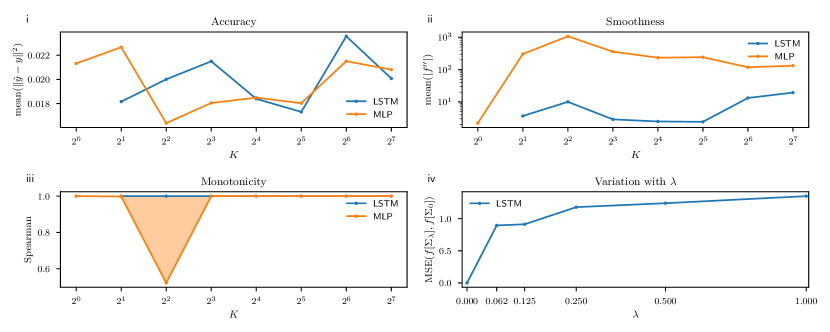
Figure 4: Results of ablation studies and validation experiments with various models. (i-iii) Variation of error, smoothness and monotonicity with K respectively. MLP models do not produce smooth, monotonic results (except K=1), and the $K=1$ MLP is outperformed by the LSTM model at roughly the same smoothness and monotonicity. (iv) Prediction variation of models trained on $\Sigma|{\lambda}$ and $\Sigma_{0}$. When the covariance matrix is progressively corrupted with noise, the predictions change, thus demonstrating our approach’s ability to model correlations.

where $\mathbf{N}=A\times{}A^{T};A_{ij}\sim\mathcal{N}(0,1)$ is a noise matrix, which is by construction symmetric and positive semi-definite. The idea is to “corrupt” the covariance matrix and study how the model predictions vary as a result (note that, $\Sigma_{0}=\Sigma_{m}$). We measured the distance between the distributions ($D_{KL}$) predicted by the model trained with $\Sigma_{\lambda}$ versus those predicted by the model trained with $\Sigma_{m}$ to see whether the predicted distributions differ. We measured $D_{KL}$, as the noisy covariance matrix is likely to affect the variance predictions as well. We observed that the distance between the predicted distribution of the model trained with $\Sigma_{\lambda}$ and $\Sigma_{0}$ increases steadily with increasing $\lambda$. This shows that the model is capable of picking up cues from the correlations between data points. These results are summarized in Figure  4 in Appendix A.

We also compare the performance of our model with other regression algorithms like k-Nearest Neighbor Regression (kNNR) and Support Vector Regression (SVR) as measured by accuracy, monotonicity and smoothness (see Table 1). In kNNR, we pick k$(=5)$ nearest instances from the training data and report a weighted sum of their corresponding target values. SVR is a variant of Support Vector Machines, and tries to find a function such that all training instances are within an $\epsilon$-interval of the function. Our algorithm and architecture, outperforms other models in accuracy while maintaining monotonicity and smoothness. Our learning algorithm, outlined in Section 3.2, alongside the architecture (LSTM, K=32) is dubbed LADDER - Learning Algorithm for Deep Distance Estimation and Reconstruction. In the subsequent sections, unless explicitly stated, we report results with this approach.

4 Cosmological Applications of Learning the Distance Ladder

Given the experimental validation of the performance of our approach in learning the distance ladder, let us now outline a few interesting cosmological applications of the algorithm, which arise as natural consequences of the training process. Of course, our intention is not to do an extensive analysis for each one, which is beyond the scope of the present article anyway. We rather intend to point out possible areas which can be explored further with LADDER, each one of them calling for detailed future investigation.

4.1 Consistency check for similar datasets in a model-independent approach

Having trained LADDER with Pantheon, we proceed to test the consistency of a comparable SNIa dataset in a model-independent manner - the Pantheon+ compilation (Scolnic et al., 2022). This compilation comprises data from 1701 light curves representing 1550 distinct SNIa over a redshift range of $0.001\lesssim{}z<2.3$. This range significantly overlaps with that of Pantheon, with a notably high data density at lower redshifts (see the left panel of Figure 1). This has significant implications for our understanding of cosmic phenomena, suggesting potential variations in the underlying astrophysical or cosmological processes. This could have a notable impact on the precision of cosmological parameter estimates and the robustness of the underlying physical model. For an unbiased assessment, we focus solely on the 753 data points in Pantheon+ which are not included in Pantheon. A comparison between these data points and the reconstructions by Pantheon-trained LADDER is presented in the right panel of Figure 1, from where a good degree of consistency is apparent.

Figure 1: Testing Pantheon+ – Relative redshift distribution of the Pantheon and Pantheon+ datasets (left panel); Comparison between Pantheon-trained LADDER reconstruction vs Pantheon+ (right panel).

Since LADDER predicts a normal distribution, we drew independent and identically distributed random samples from LADDER predictions and the Pantheon+ dataset, to perform a t-test. We found with an extremely high degree of certainty (mean p-value 0.00245) that the predicted and observed distributions are similar. This confirms the validity of doing cosmology by incorporating Pantheon into the full Pantheon+ dataset (Brout et al., 2022), within the precision of LADDER predictions. Comparison of constraints obtained on cosmological model parameters using Markov Chain Monte Carlo (MCMC) may serve as additional tests of consistency, and we hope to do a detailed analysis along these lines in the near future.

Consistency tests, such as these, can be extended to upcoming SNIa datasets, including the recent Dark Energy Survey 5-Year Data Release announcement (Abbott et al., 2024). This dataset comprises 1829 SNIa in the redshift range of $0.10<z<1.13$, exhibiting a higher data density at higher redshifts compared to Pantheon+. The anticipated release of the actual data holds the potential for an exciting validation study of our ML approach. Furthermore, SNIa datasets from upcoming missions such as Euclid (Amendola et al., 2013), Rubin LSST (Zhan & Tyson, 2018), Roman Space Telescope (Akeson et al., 2019), the Thirty Meter Telescope (TMT) (Skidmore et al., 2015), and the already launched James Webb Space Telescope (JWST) (Gardner et al., 2006) can serve as valuable resources for future efforts towards consistency checks.

4.2 Pathology test for different datasets in apparent tension

Since LADDER does not depend on a cosmological model, it can serve as a model-independent test for different types of data, especially those in the same redshift range as the SNIa dataset used for training. Such checks are relevant given the persistent tensions between different datasets. Here, we outline a sketch of the procedure for this with the BAO datasets. In contrast to SNIa measurements, which infer luminosity distances ($d_{L}$) from apparent magnitude values ($m$) by assuming an absolute magnitude ($M_{B}$), BAO measures angular distances $d_{A}/r_{d}$. The cosmic-distance duality relation, $d_{A}(z)=(1+z)^{-2}d_{L}(z)$, connects these quantities, with $r_{d}$ being the co-moving sound horizon at the drag epoch, which needs to be calibrated for cosmological applications.

Typically, BAO measurements are combined with CMB data, which can tightly constrain $r_{d}$ thereby breaking the degeneracy between $r_{d}$ and $d_{A}$. In this study, we utilize BAO measurements to establish a connection between SNIa and CMB observations. We calibrate the angular distance from BAO with the LADDER predictions in a model-independent way. This enables the propagation of the CMB constraint on $r_{d}$ into a constraint on $M_{B}$, or the SH0ES-prior on $M_{B}$ into a constraint on $r_{d}$. We attempt this exercise for two different sets of BAO data:

• Transverse Angular BAO ($\theta_{\text{BAO}}$), comprising of 15 model-independent data points in the redshift range $0.11\lesssim{}z\lesssim 2.22$, taken from the compilation in Nunes et al. (2020), obtained from SDSS-III LRGs, SDSS-IV blue galaxies and quasars.

• Anisotropic BAO ($\alpha_{\text{BAO}}$), consisting of 8 Galaxy+Ly$\alpha$ data points in the redshift range $0.38\lesssim{}z\lesssim 2.35$, from the SDSS-III, SDSS-IV DR12 and DR14 data releases, as outlined in Dialektopoulos et al. (2023).

Figure 2: Calibration of BAO – Colored contours are LADDER predictions, dashed ones correspond to benchmark $\Lambda$CDM calibration.

Initially, we assume different choices of $M_{B}\in\left[-19.5,-19.1\right]$ and constrain $r_{d}$ by minimizing the $\chi^{2}$ metric between the BAO data and the mean LADDER predictions at the corresponding redshifts, taking into account the full covariances associated with the BAO datasets. The direct correlation between the two calibrating parameters is evident from the monotonicity of the constraints depicted in the left-most panel of Figure 2.

However, it is noteworthy that discordant constraints on $r_{d}$ exist between the two BAO datasets for a given value of $M_{B}$. This discrepancy may imply an internal inconsistency between angular and anisotropic BAO measurements, possibly attributed to the $\Lambda$CDM model dependence in anisotropic BAO data (Carter et al., 2020), an aspect that calls for further study.

We find out the difference between the vanilla $\Lambda$CDM model-dependent BAO calibration, versus our LADDER based model-independent calibration. In the middle panel of Figure 2, we show the joint constraints on the parameters $M_{B}$ and $r_{d}$ given different choices of priors - an astrophysical prior on $M_{B}^{\text{SH0ES}}=-19.2478\pm 0.0294$ (Scolnic et al., 2018) and the Planck 2018 CMB prior on $r_{d}^{\text{CMB}}=147.09\pm 0.26$ Mpc (Aghanim et al., 2020), thus breaking the degeneracy between both the parameters. Here SN refers to the Pantheon dataset. The colored contours depict LADDER mean predictions, and the dotted contours are for $\Lambda$CDM. The consistency between the two, albeit with very minor variations, suggests that the true cosmology might resemble something close to the $\Lambda$CDM model. However, the tension between angular vs anisotropic BAO measurements is apparent for both methods of calibration here, which is of considerable concern.

Table 2: Comparison between constraints on $M_{B}$ and $r_{d}$ [in Mpc], employing LADDER vs vanilla $\Lambda$CDM model.

Datasets	LADDER		$\Lambda$CDM
	$M_{B}$	$r_{d}$	$H_{0}$	$\Omega_{m0}$	$M_{B}$	$r_{d}$
SN+$\alpha_{\text{BAO}}$+$M_{B}^{\text{SH0ES}}$	$-19.249^{+0.029}_{-0.029}$	$137.651^{+2.157}_{-2.153}$	$73.195_{-1.032}^{+1.054}$	$0.315_{-0.019}^{+0.019}$	$-19.248_{-0.029}^{+0.030}$	$137.484_{-2.228}^{+2.312}$
SN+$\theta_{\text{BAO}}$+$M_{B}^{\text{SH0ES}}$	$-19.248^{+0.028}_{-0.029}$	$146.423^{+2.697}_{-2.569}$	$73.372_{-1.010}^{+1.023}$	$0.302_{-0.021}^{+0.022}$	$-19.248_{-0.029}^{+0.028}$	$147.246_{-2.712}^{+2.795}$
SN+$\alpha_{\text{BAO}}$+$r_{d}^{\text{CMB}}$	$-19.394^{+0.018}_{-0.017}$	$147.090^{+0.250}_{-0.267}$	$68.437_{-0.826}^{+0.820}$	$0.314_{-0.019}^{+0.020}$	$-19.394_{-0.022}^{+0.021}$	$147.087_{-0.256}^{+0.258}$
SN+$\theta_{\text{BAO}}$+$r_{d}^{\text{CMB}}$	$-19.257^{+0.028}_{-0.027}$	$147.085^{+0.261}_{-0.253}$	$73.448_{-1.025}^{+1.042}$	$0.304_{-0.021}^{+0.022}$	$-19.245_{-0.027}^{+0.028}$	$147.088_{-0.256}^{+0.259}$

So, we further our pathology test by incorporating the 1$\sigma$ uncertainty predictions from LADDER and redo the above exercise. Notably, the LADDER-based contours widen significantly (see right panel of Figure 2). Given uncalibrated Pantheon data, LADDER predicts a minimum as well as a maximum contour spread in comparison to the $\Lambda$CDM model. This data-driven selection of the $M_{B}$-$r_{d}$ parameter space can serve as a consistency check for similar exercises with arbitrary models, to be well constrained with Pantheon SN+BAO data.

It’s imperative to recall that values of $M_{B}$ and $r_{d}$ significantly influence $H_{0}$ (Chen et al., 2024), hence they need to be chosen with much care in the context of the prevalent Hubble tension. The contour plots in Figure 2 suggest no apparent tension between Pantheon and $\theta_{\text{BAO}}$ datasets, unlike $\alpha_{\text{BAO}}$. Thus, for any cosmological analysis, the use of angular BAO data, instead of anisotropic BAO, can be recommended as long as late-time datasets are considered in conjunction. Having said that, we should leave a word of caution here. While Table 2 suggests an apparent resolution of the $H_{0}$ tension, an exhaustive Planck CMB analysis is necessary before drawing firm conclusions.

4.3 Model-independent calibration of high-redshift datasets

Datasets that can potentially yield $d_{L}$, but lack calibration through well-established anchors in the distance ladder, need to be calibrated by either assuming a cosmological model (Dai et al., 2004) or by some model-independent (Liang et al., 2008) means. A relevant example involves observations of GRBs which tabulate the GRB spectral peak energy $E^{\text{obs}}_{p}$ and bolometric fluence $S_{\text{bolo}}$ at different redshifts.

We investigate if LADDER, trained on uncalibrated Pantheon, can serve as a reliable model-independent calibrator for GRBs. This approach alleviates the challenge of selecting a specific cosmological model for calibration, enabling LADDER-calibrated GRBs as a unique dataset to constrain parameters across diverse cosmological models, avoiding the so-called circularity problem (Ghirlanda et al., 2006).

To demonstrate this, we use the GRB A219 sample as outlined in Liang et al. (2022) spanning the redshift range $0.03<z\lesssim 8.2$, which correlates the spectral peak energy ($E_{p}$) and the isotropic equivalent radiated energy ($E_{\text{iso}}$) following Amati relation (Amati et al., 2002) as follows,

$$\log_{10}\frac{E_{\text{iso}}}{\text{1~{}erg}}=a+b\,\log_{10}\frac{E_{p}}{\text{300~{}keV}}\>.$$ (15)

Here, $a$ and $b$ are free coefficients, which connects the GRB observables to cosmic distance, such that $E_{\text{iso}}=4\pi{}d^{2}_{L}(z)S_{\text{bolo}}(1+z)^{-1}$ and $E_{p}=E^{\text{obs}}_{p}(1+z)$. We then split this GRB data into low-redshift ($z<1.5$) and high-redshift ($z>1.5$) samples, consisting of 89 and 130 points respectively. Since LADDER predicts $m$ directly, we express the GRB relation in terms of the same without assuming any prior values of $M_{B}$ (equation (1)). To this end, the Amati relation is rewritten as, $y^{\prime}=~{}a^{\prime}+b\,x$, where $y^{\prime}=\log_{10}\left[(1+z)^{-1}\left({S_{\text{bolo}}/{1\text{erg~{}cm}^{-2}}}\right)\right]+\frac{2}{5}m$. So, $a^{\prime}=a+2\left(\frac{M_{B}}{5}+5\right)-\log_{10}\left[4\pi\textrm{(Mpc/cm)}^{2}\right]$ and $b$ are now the free coefficients to be calibrated given $m$ vs $z$ (Zhang et al., 2023). We use the likelihood function by Reichart (2001) to fit the parameters $a^{\prime}$ and $b$, using the low-$z$ GRB sample. Since LADDER has been trained to learn the distance ladder properly, we then construct a high-$z$ GRB dataset, as shown in the left panel of Figure 3.

Figure 3: GRB calibration output and comparisons.

With this model-independent high-$z$ GRB dataset we obtain constraints on parameter spaces of two cosmological models - baseline $\Lambda$CDM and the wCDM model. For the MCMC analysis, we also incorporate the 32 Cosmic Chronometer (CC) Hubble parameter measurements, as listed in Dialektopoulos et al. (2023), along with the full covariance matrix including the systematic and calibration errors (Moresco et al., 2020), covering the redshift range up to $z\lesssim 2$. The results are shown in the right panel of Figure 3. Besides LADDER, for comparison, we further calibrate the Amati coefficients employing both the above-mentioned cosmological models assuming the Pantheon SNIa + Planck2018 CMB + BAO (PCB) best-fit model parameter values, following which we work out the full analysis with the respective model-calibrated datasets.

Table 3: GRB constraints on cosmological models.

Model	$\Lambda$CDM		wCDM
Calibrator	LADDER	PCB	LADDER	PCB
$H_{0}$	$69.203_{-4.150}^{+4.050}$	$68.996_{-4.095}^{+4.187}$	$71.224_{-6.365}^{+9.058}$	$70.265_{-5.915}^{+8.989}$
$\Omega_{m0}$	$0.313_{-0.055}^{+0.066}$	$0.317_{-0.057}^{+0.067}$	$0.289_{-0.074}^{+0.068}$	$0.287_{-0.085}^{+0.072}$
$w_{0}$	…	…	$-1.257_{-0.867}^{+0.627}$	$-1.172_{-0.866}^{+0.599}$

We find that the constraints obtained for $\Lambda$CDM are consistent, irrespective of the calibration method, with only a marginal widening of errors for the model-independent LADDER calibration. Similar conclusions hold when considering a beyond-$\Lambda$CDM model such as $w$CDM. This suggests that regardless of the cosmological model to be constrained, calibration via LADDER can provide a unique high-$z$ GRB dataset in a model-independent setting. Further, Table 3 indicates an apparent trend towards higher $H_{0}$ values, despite not using any local $H_{0}$ prior in our analysis. While the associated uncertainties remain considerable, the observed mean shifts in $H_{0}$ are slightly more pronounced with the implementation of LADDER, compared to the outcomes obtained through model-based calibration. This disparity warrants further investigation and analysis.

GRBs are not the only challenging high-redshift datasets that need calibration independently of any cosmological model. Distance measurements involving high-redshift quasars (Dainotti et al., 2024) and early observations from the recently launched JWST (Boylan-Kolchin, 2023) may also be potential candidates for the application of LADDER calibration.

4.4 Other possible applications and future directions

The persistent tension between $H_{0}$ inferred from early-time probes, assuming vanilla $\Lambda$CDM, with the directly measured $H_{0}$ from late-time observations, suggests a potential need for an alternative cosmological model. Various proposals exist in the literature (Di Valentino et al., 2021; Schöneberg et al., 2022; Abdalla et al., 2022), but none fully reconcile CMB-based model-dependent measurements with late-time direct measurements. LADDER offers the opportunity to constrain such alternative models using a broader range of datasets.

LADDER’s reasonable extrapolation feature to higher redshifts enables generation of synthetic diverse and augmented datasets. This will in particular be useful for cosmological forecast studies with upcoming gravitational wave missions, such as LISA (Tamanini et al., 2016), ET (Maggiore et al., 2020) and DECIGO (Mandel et al., 2018), which often requires generating mock catalogs, inherently relying on a fiducial choice of a cosmological model (Shah et al., 2023; Mukherjee et al., 2024). We propose that our algorithm could be used as a mock data generator, based solely on the real Pantheon dataset and an assumed value of $M_{B}$.

Another major cosmological goal is the direct reconstruction of the Hubble parameter. This requires predictions on not just $d_{L}$, but also its derivatives $d_{L}^{\prime}$, with associated errors. GP inherently handle this task by allowing analytical predictions of derivatives and errors, however, they struggle in data-scarce regions and completely fail where no data is available. Neural networks, despite being more performant, do not natively model $d_{L}^{\prime}$ and its associated error $\sigma_{d_{L}^{\prime}}$. Although attempts to numerically differentiate the network outputs for $d_{L}$ have been undertaken (Mukherjee et al., 2022; Dialektopoulos et al., 2023, 2024), these lead to substantially large uncertainties, rendering final results ineffective when it comes to precision cosmology at higher redshifts. Experiments with LADDER have shown early promise in this regard, and we plan on expanding upon this in the future.

5 Conclusion

The lack of reliable data points at high redshifts, and the smoothness of the expansion history of our Universe, makes deep learning network models prone to overfitting/underfitting issues, which significantly leads to both inaccurate and imprecise predictions. We hence propose a novel approach in using a deep learning algorithm that learns sequential data while utilizing the full covariance information among data points, applied to cosmological datasets. Our method, part of the new LADDER (Learning Algorithm for Deep Distance Estimation and Reconstruction) suite, is trained on uncalibrated SNIa data from the Pantheon compilation in a manner that is robust to outliers and noise; whilst showing appreciable precision. Our validation experiments show that LSTMs outperform other architectures and ML frameworks in performance and smoothness, perhaps suggesting the importance of capturing the sequential nature of the dataset. The resulting network also exhibits stability, even in data-sparse regions, and enables reliable predictions with associated error bars extending reliably to somewhat beyond the training data range.

Our approach shows promise for contributing to the reconstruction of the cosmic distance ladder in a model-independent manner, as opposed to the conventional cosmological model-dependent approach, with potential applications including the validation of similar SNIa datasets, cross-validation with other observational data, and calibration of high-redshift measurements. Furthermore, our network could serve as a mock-data generator, capable of reasonable extrapolation without succumbing to overfitting. This capability opens avenues for generating model-independent, Pantheon-based data, at higher redshifts, which is crucial for forecast studies with upcoming cosmological observatories.

While we recognize other approaches, we want to gently emphasize the potential benefits of using advanced learning techniques and attempt to demonstrate how they can optimize information extraction from cosmological data. We hence wish to underscore the innovative nature of employing this new learning algorithm within the cosmological framework and extend our encouragement to the community to consider adopting this algorithm for extracting comprehensive information from cosmological data. We also reiterate that there can be some yet unexplored deep learning algorithm that may perform even better than ours. This work might encourage the community to explore them in different contexts of cosmology. Such efforts would significantly impact the accuracy and reliability of the reconstruction methods and help address yet unresolved issues of cosmology from a different perspective.

6 Software and third party data repository citations

The LADDER (Learning Algorithm for Deep Distance Estimation and Reconstruction) suite and data for this article are available on GitHub: https://github.com/rahulshah1397/LADDER, and will be made public once the paper is accepted.

Appendix A Training Algorithm and Validation

 LADDER - Learning Algorithm for Deep Distance Reconstruction and Estimation

Given $\mathcal{D},\mathbf{C}_{\text{sys}}$ and batch size $B$.

Initialize $\theta_{0}$.

while not StopCondition do

     $l\leftarrow 0$

     for $i=1,2,\ldots{}B$ do

         $\text{Get }K\text{ samples from }\mathcal{D}$

         $\quad\quad\{(z_{1},m_{1},\Delta{}m_{1}),\ldots(z_{K},m_{K},\Delta{}m_{K})\}$

         $Y_{i}=(m_{j_{1}},\Delta{}m_{j_{1}})$

         $\hat{m}_{j_{2}},\hat{m}_{j_{3}},\ldots\hat{m}_{j_{K}}\sim\mathcal{N}(m_{j_{2}},m_{j_{3}},\ldots{}m_{j_{K}},\Sigma_{m}^{K})$ $\triangleright$ (equation (9))

         $X_{i}=(z_{j_{1}},z_{j_{2}},\hat{m}_{j_{2}},\ldots{}z_{j_{K}},\hat{m}_{j_{K}})\quad{}z_{j_{2}}\leq{}z_{j_{3}}\ldots$

         $\mu,\sigma=f_{\theta_{t}}(X_{i})_{1},f_{\theta_{t}}(X_{i})_{2}$$\triangleright$ Forward pass.

         $l\mathrel{+}=D_{KL}\Big{(}\mathcal{N}(m_{j_{1}},\Delta{}m_{j_{1}}),\mathcal{N}(\mu,\sigma)\Big{)}$

     end for

     Compute $\nabla_{\theta_{t}}l\quad\forall\theta_{t}$

     $\theta_{t+1}=\theta_{t}+\eta\cdot\nabla_{\theta_{t}}$$\triangleright$ Gradient update (illustrative).

     if $\ldots$ then$\triangleright$ Check if model converged.

         StopCondition $\leftarrow$ True

     end if

end while

References

- Abbott et al. (2024) Abbott, T. M. C., et al. 2024, arXiv. https://arxiv.org/abs/2401.02929
- Abdalla et al. (2022) Abdalla, E., et al. 2022, JHEAp, 34, 49, doi: 10.1016/j.jheap.2022.04.002
- Aghanim et al. (2020) Aghanim, N., et al. 2020, Astron. Astrophys., 641, A6, doi: 10.1051/0004-6361/201833910
- Akeson et al. (2019) Akeson, R., et al. 2019, arXiv:1902.05569, doi: 10.48550/arXiv.1902.05569
- Amati et al. (2002) Amati, L., et al. 2002, Astron. Astrophys., 390, 81, doi: 10.1051/0004-6361:20020722
- Amendola et al. (2013) Amendola, L., et al. 2013, Living Rev. Rel., 16, 6, doi: 10.12942/lrr-2013-6
- Arjona et al. (2021) Arjona, R., Lin, H.-N., Nesseris, S., & Tang, L. 2021, Phys. Rev. D, 103, 103513, doi: 10.1103/PhysRevD.103.103513
- Bernal et al. (2016) Bernal, J. L., Verde, L., & Riess, A. G. 2016, JCAP, 10, 019, doi: 10.1088/1475-7516/2016/10/019
- Boylan-Kolchin (2023) Boylan-Kolchin, M. 2023, Nature Astron., 7, 731, doi: 10.1038/s41550-023-01937-7
- Brout et al. (2022) Brout, D., et al. 2022, Astrophys. J., 938, 110, doi: 10.3847/1538-4357/ac8e04
- Camarena & Marra (2020) Camarena, D., & Marra, V. 2020, Mon. Not. Roy. Astron. Soc., 495, 2630, doi: 10.1093/mnras/staa770
- Capozziello et al. (2018) Capozziello, S., D’Agostino, R., & Luongo, O. 2018, Mon. Not. Roy. Astron. Soc., 476, 3924, doi: 10.1093/mnras/sty422
- Carter et al. (2020) Carter, P., Beutler, F., Percival, W. J., et al. 2020, Mon. Not. Roy. Astron. Soc., 494, 2076, doi: 10.1093/mnras/staa761
- Chen et al. (2024) Chen, Y., Kumar, S., & Ratra, B. 2024, arXiv. https://arxiv.org/abs/2401.13187
- Cuesta et al. (2015) Cuesta, A. J., Verde, L., Riess, A., & Jimenez, R. 2015, Mon. Not. Roy. Astron. Soc., 448, 3463, doi: 10.1093/mnras/stv261
- Dai et al. (2004) Dai, Z. G., Liang, E. W., & Xu, D. 2004, Astrophys. J. Lett., 612, L101, doi: 10.1086/424694
- Dainotti et al. (2024) Dainotti, M. G., Bargiacchi, G., Lenart, A. L., & Capozziello, S. 2024, arXiv. https://arxiv.org/abs/2401.11998
- Di Valentino et al. (2021) Di Valentino, E., Mena, O., Pan, S., et al. 2021, Class. Quant. Grav., 38, 153001, doi: 10.1088/1361-6382/ac086d
- Dialektopoulos et al. (2023) Dialektopoulos, K. F., Mukherjee, P., Levi Said, J., & Mifsud, J. 2023, Eur. Phys. J. C, 83, 956, doi: 10.1140/epjc/s10052-023-12124-3
- Dialektopoulos et al. (2024) —. 2024, Phys. Dark Univ., 43, 101383, doi: 10.1016/j.dark.2023.101383
- Escamilla-Rivera et al. (2022) Escamilla-Rivera, C., Carvajal, M., Zamora, C., & Hendry, M. 2022, JCAP, 04, 016, doi: 10.1088/1475-7516/2022/04/016
- Foreman-Mackey et al. (2013) Foreman-Mackey, D., Hogg, D. W., Lang, D., & Goodman, J. 2013, Publ. Astron. Soc. Pac., 125, 306, doi: 10.1086/670067
- Freedman & Madore (2023) Freedman, W. L., & Madore, B. F. 2023, arXiv. https://arxiv.org/abs/2308.02474
- Freedman et al. (2020) Freedman, W. L., Madore, B. F., Hoyt, T., et al. 2020, arXiv, doi: 10.3847/1538-4357/ab7339
- Gardner et al. (2006) Gardner, J. P., Mather, J. C., Clampin, M., et al. 2006, Space Science Reviews, 123, 485, doi: 10.1007/s11214-006-8315-7
- Ghirlanda et al. (2006) Ghirlanda, G., Ghisellini, G., & Firmani, C. 2006, New J. Phys., 8, 123, doi: 10.1088/1367-2630/8/7/123
- Giambagli et al. (2023) Giambagli, L., Fanelli, D., Risaliti, G., & Signorini, M. 2023, Astron. Astrophys., 678, A13, doi: 10.1051/0004-6361/202346236
- Gómez-Vargas et al. (2023a) Gómez-Vargas, I., Andrade, J. B., & Vázquez, J. A. 2023a, Phys. Rev. D, 107, 043509, doi: 10.1103/PhysRevD.107.043509
- Gómez-Vargas et al. (2023b) Gómez-Vargas, I., Esquivel, R. M., García-Salcedo, R., & Vázquez, J. A. 2023b, Eur. Phys. J. C, 83, 304, doi: 10.1140/epjc/s10052-023-11435-9
- Hazra et al. (2015) Hazra, D. K., Majumdar, S., Pal, S., Panda, S., & Sen, A. A. 2015, Phys. Rev. D, 91, 083005, doi: 10.1103/PhysRevD.91.083005
- Hochreiter & Schmidhuber (1997) Hochreiter, S., & Schmidhuber, J. 1997, Neural Comput., 9, 1735–1780, doi: 10.1162/neco.1997.9.8.1735
- Hornik et al. (1989) Hornik, K., Stinchcombe, M., & White, H. 1989, Neural Networks, 2, 359, doi: https://doi.org/10.1016/0893-6080(89)90020-8
- Hwang et al. (2023) Hwang, S.-g., L’Huillier, B., Keeley, R. E., Jee, M. J., & Shafieloo, A. 2023, JCAP, 02, 014, doi: 10.1088/1475-7516/2023/02/014
- Keeley et al. (2021) Keeley, R. E., Shafieloo, A., Zhao, G.-B., Vazquez, J. A., & Koo, H. 2021, Astron. J., 161, 151, doi: 10.3847/1538-3881/abdd2a
- Liang et al. (2022) Liang, N., Li, Z., Xie, X., & Wu, P. 2022, Astrophys. J., 941, 84, doi: 10.3847/1538-4357/aca08a
- Liang et al. (2008) Liang, N., Xiao, W. K., Liu, Y., & Zhang, S. N. 2008, Astrophys. J., 685, 354, doi: 10.1086/590903
- Maggiore et al. (2020) Maggiore, M., et al. 2020, JCAP, 03, 050, doi: 10.1088/1475-7516/2020/03/050
- Mandel et al. (2018) Mandel, I., Sesana, A., & Vecchio, A. 2018, Class. Quant. Grav., 35, 054004, doi: 10.1088/1361-6382/aaa7e0
- Moresco et al. (2020) Moresco, M., Jimenez, R., Verde, L., Cimatti, A., & Pozzetti, L. 2020, Astrophys. J., 898, 82, doi: 10.3847/1538-4357/ab9eb0
- Mukherjee et al. (2022) Mukherjee, P., Levi Said, J., & Mifsud, J. 2022, JCAP, 12, 029, doi: 10.1088/1475-7516/2022/12/029
- Mukherjee & Mukherjee (2021) Mukherjee, P., & Mukherjee, A. 2021, Mon. Not. Roy. Astron. Soc., 504, 3938, doi: 10.1093/mnras/stab1054
- Mukherjee et al. (2024) Mukherjee, P., Shah, R., Bhaumik, A., & Pal, S. 2024, Astrophys. J., 960, 61, doi: 10.3847/1538-4357/ad055f
- Novosyadlyj et al. (2014) Novosyadlyj, B., Sergijenko, O., Durrer, R., & Pelykh, V. 2014, JCAP, 05, 030, doi: 10.1088/1475-7516/2014/05/030
- Nunes et al. (2020) Nunes, R. C., Yadav, S. K., Jesus, J. F., & Bernui, A. 2020, Mon. Not. Roy. Astron. Soc., 497, 2133, doi: 10.1093/mnras/staa2036
- Ó Colgáin & Sheikh-Jabbari (2021) Ó Colgáin, E., & Sheikh-Jabbari, M. M. 2021, Eur. Phys. J. C, 81, 892, doi: 10.1140/epjc/s10052-021-09708-2
- Olvera et al. (2022) Olvera, J. d. D. R., Gómez-Vargas, I., & Vázquez, J. A. 2022, Universe, 8, 120, doi: 10.3390/universe8020120
- Reichart (2001) Reichart, D. E. 2001, The Astrophysical Journal, 553, 235, doi: 10.1086/320630
- Riess & Breuval (2023) Riess, A. G., & Breuval, L. 2023, arXiv. https://arxiv.org/abs/2308.10954
- Sanger & Baljekar (1958) Sanger, T., & Baljekar, P. N. 1958, Psychological review, 65 6, 386. https://api.semanticscholar.org/CorpusID:12781225
- Schöneberg et al. (2022) Schöneberg, N., Franco Abellán, G., Pérez Sánchez, A., et al. 2022, Phys. Rept., 984, 1, doi: 10.1016/j.physrep.2022.07.001
- Scolnic et al. (2022) Scolnic, D., et al. 2022, Astrophys. J., 938, 113, doi: 10.3847/1538-4357/ac8b7a
- Scolnic et al. (2018) Scolnic, D. M., Jones, D. O., Rest, A., et al. 2018, Astrophys. J., 859, 101, doi: 10.3847/1538-4357/aab9bb
- Shah et al. (2023) Shah, R., Bhaumik, A., Mukherjee, P., & Pal, S. 2023, JCAP, 06, 038, doi: 10.1088/1475-7516/2023/06/038
- Sherwin & White (2019) Sherwin, B. D., & White, M. 2019, JCAP, 02, 027, doi: 10.1088/1475-7516/2019/02/027
- Skidmore et al. (2015) Skidmore, W., et al. 2015, Res. Astron. Astrophys., 15, 1945, doi: 10.1088/1674-4527/15/12/001
- Tamanini et al. (2016) Tamanini, N., et al. 2016, J. Cosmol. Astropart. Phys., 2016, 002, doi: 10.1088/1475-7516/2016/04/002
- Visser (2005) Visser, M. 2005, Gen. Rel. Grav., 37, 1541, doi: 10.1007/s10714-005-0134-8
- Wang et al. (2020) Wang, G.-J., Ma, X.-J., Li, S.-Y., & Xia, J.-Q. 2020, Astrophys. J. Suppl., 246, 13, doi: 10.3847/1538-4365/ab620b
- Wei et al. (2014) Wei, H., Yan, X.-P., & Zhou, Y.-N. 2014, JCAP, 01, 045, doi: 10.1088/1475-7516/2014/01/045
- Zhan & Tyson (2018) Zhan, H., & Tyson, J. A. 2018, Reports on Progress in Physics, 81, 066901, doi: 10.1088/1361-6633/aab1bd
- Zhang et al. (2023) Zhang, B., Xie, X., Nong, X., et al. 2023, arXiv. https://arxiv.org/abs/2312.09440
- Zhang et al. (2017) Zhang, C., Bengio, S., Hardt, M., Recht, B., & Vinyals, O. 2017, in International Conference on Learning Representations. https://openreview.net/forum?id=Sy8gdB9xx
- Zhang et al. (2024) Zhang, J.-C., Hu, Y., Jiao, K., et al. 2024, Astrophys. J. Suppl., 270, 23, doi: 10.3847/1538-4365/ad0f1e