A Unified Three-State Model Framework for Analysis of Treatment Crossover in Survival Trials

Abstract

We present a unified three-state model (TSM) framework for evaluating treatment effects in clinical trials in the presence of treatment crossover. Researchers have proposed diverse methodologies to estimate the treatment effect that would have hypothetically been observed if treatment crossover had not occurred. However, there is little work on understanding the connections between these different approaches from a statistical point of view. Our proposed TSM framework unifies existing methods, effectively identifying potential biases, model assumptions, and inherent limitations for each method. This can guide researchers in understanding when these methods are appropriate and choosing a suitable approach for their data. The TSM framework also facilitates the creation of new methods to adjust for confounding effects from treatment crossover. To illustrate this capability, we introduce a new imputation method that falls under its scope. Using a piecewise constant prior for the hazard, our proposed method directly estimates the hazard function with increased flexibility. Through simulation experiments, we demonstrate the performance of different approaches for estimating the treatment effects.

Keywords: intention-to-treat, piecewise constant hazard, survival trials, treatment crossover

1 Introduction

Randomized controlled trials (RCTs) have been commonly used to compare the survival outcomes between a treatment group and a control group. Treatment crossover within an RCT takes place when patients randomized to a treatment or control group switch to a different group from the one to which they were initially assigned (Ishak et al., 2014; Jönsson et al., 2014; Watkins et al., 2013).

Treatment crossover can occur for a variety of reasons and can be either noninformative or informative. We define noninformative crossover as any scenario where patients switch treatments for reasons unrelated to treatment efficacy, disease progression, or any meaningful clinical factors. An example of noninformative crossover is a study protocol which allows patients in the control group to switch to the experimental treatment once the main study endpoint (e.g. the blinded phase of the trial) has been reached (Daugherty et al., 2008). For example, in the CENTAUR trial of sodium phenylbutyrate and taurursodio (PB and TURSO) in amyotrophic lateral sclerosis (ALS), patients in the control group all switched to the experimental treatment after they completed the 24-week double-blind study phase (Paganoni et al., 2022).

However, treatment crossover can also be informative. Informative crossover occurs when patients switch treatments as a result of disease progression (Ishak et al., 2014; Latimer et al., 2014). Informative treatment crossover is often a selective process. For example, only patients who are deemed the most likely to benefit from the experimental treatment may be crossed over, while those who have reached the terminal stage of the disease typically are not (Ishak et al., 2014). In many real-life scenarios, crossover can also result from a mixture of both noninformative and informative events, such as the other treatment arm being perceived to be better and a sudden change in the patient’s condition (Ishak et al., 2011).

These diverse scenarios invariably introduce complications in data analysis to estimate the treatment efficacy. Under treatment crossover, conventional statistical techniques such as intention-to-treat analysis (Brody, 2016) (described in Section 3) may yield biased estimations of the true treatment effect. To illustrate this, we consider the following example. Progression-free survival (PFS) is a commonly used clinical endpoint, particularly in Oncology (Dancey et al., 2009). PFS measures the duration between randomization and disease progression or death. Post-progression survival (PPS) refers to the time after disease progression to death. Figure 1 shows that the survival time for a crossovered patient represents a mixed effect of having received both the control and experimental treatments. The observed difference in survival time is biased as a result of this contamination, and the true treatment effect is underestimated (Ishak et al., 2014; Latimer et al., 2014).

Figure 1: Diagram of PFS and PPS for patients assigned to the control, experimental, and crossovered treatments

An intuitive approach to account for treatment crossover is to exclude or censor data at the point of crossover. This is also known as the per-protocol method (Brody, 2016), where researchers only focus on PFS when crossover is linked with the disease progression. However, the per-protocol method can be vulnerable to selection bias, as individuals who switched from the control treatment to the experimental treatment might have different prognoses and therefore are not “exchangeable” with patients who stayed in the control group (Arnold & Ercumen, 2016). Potential solutions such as randomized crossover designs can be applied to mitigate the effects of selection bias (McKeever, 2021; Simon & Chinchilli, 2007). However, randomization – while effective in theory – is not always practical or ethical (Simon & Chinchilli, 2007). A more pragmatic approach may be to adjust for crossover effects within the statistical analysis.

Numerous approaches for estimating the true treatment effect (or hazard ratio) in the presence of treatment crossover have been proposed and examined. In Section 3, we describe several of the most popular methods. Morden et al. (2011) and Latimer et al. (2018) conducted simulations in a variety of plausible crossover scenario settings and compared the results from these different methods. Other recent reviews covering a range of therapeutic areas can be found in Watkins et al. (2013), Ishak et al. (2014), and Jönsson et al. (2014).

Despite these reviews and comparative studies, there is little work on understanding how these different methods relate to each other in terms of their statistical properties. While assessing these methods’ performance under various simulation settings (Morden et al., 2011; Latimer et al., 2018) is certainly illuminating, it is not always straightforward for practitioners to know which statistical method they should use to adjust for confounding from treatment crossover. Moreover, based on domain knowledge or evidence from past trials, a researcher may also want to incorporate their own assumptions (e.g. an assumption that the treatment effect is constant over time) into their statistical analyses (Kahan & Morris, 2013; Glidden et al., 2020).

In this paper, we propose to use a three-state model (TSM) framework to synthesize existing statistical methods in treatment crossover analysis. In addition to unifying existing methods under one statistical umbrella, our TSM framework easily enables the creation of new methods allowing the incorporation of diverse assumptions tailored to specific scenarios. We demonstrate the utility of the TSM framework by introducing a novel method for estimating the hazard function. We find that all methods rely on critical limiting assumptions, and the accuracy of estimating the treatment effect relies on the validity of these assumptions. Our framework can guide practitioners in determining (or inventing) the most appropriate method to use for analyzing their data from clinical trials with treatment crossover.

The rest of this paper is structured as follows. Section 2 formally introduces the TSM framework. Section 3 places existing methods in the context of this framework and introduces a new imputation method. Section 4 demonstrates the methodologies through simulation experiments. Section 5 concludes the paper with a brief discussion.

2 Three-State Model Framework for Treatment Crossover

The main thrust of this article is to introduce a broad statistical framework for understanding the assumptions, limitations, and relationships of different methods for estimating treatment effects in RCTs with treatment crossover. We first introduce the TSM framework and discuss treatment effect estimation under this framework.

2.1 Statistical Framework

In an RCT, we define the entry as the time that a patient enters the trial. Let $T$ be the time from entry to the event of interest (e.g. death), and let $U$ be the time from entry to the time of crossover. Patients can arrive at the event of interest in two potential pathways. The first is to go to the event directly from entry without crossover, characterized by a hazard function $\lambda_{1}(t)$. The second path is where a crossover point (e.g. re-randomization, progression, or end of the double-blind phase) occurs. In this scenario, we let $\lambda_{2}^{\bf x}(t\mid u)$ denote the hazard function from crossover to the event. The crossover path is completed with the path connecting the entry point and the crossover point, and we represent the hazard function for this path as $\lambda_{3}(u)$. Figure 2 depicts these paths. Formally, the three hazard functions are defined as follows:

Figure 2: Diagram of the three-state model

(1) hazard from entry to event without crossover:

$$\lambda_{1}(t)=P(T=t\mid T\geq t,U\geq t),\hskip 14.22636ptt>0.$$ (1)

(2) hazard from crossover to event (if there is crossover):

$$\lambda^{\bf x}_{2}(t\mid u)=P(T=t\mid T\geq t,U=u),\hskip 14.22636ptt>u.$$ (2)

(3) hazard from entry to crossover:

$$\lambda_{3}(u)=P(U=u\mid T\geq u,U\geq u),\hskip 14.22636ptu>0.$$ (3)

We assume $U=\infty$ when $U>T$, i.e. crossover occurring after the event cannot be observed or is of no interest. Often times, we are interested in the survival function $\widetilde{S}(t)=P(T>t)$. Routine calculations give

$$\widetilde{S}(t) =P(T>t,U>t)+P(T>t\geq U)$$

$$=S_{1}(t)S_{3}(t)+\int_{0}^{t}P(T>t,T\geq u,U=u)du$$

$$=S_{1}(t)S_{3}(t)+\int_{0}^{t}\exp\Big{\{}-\int_{u}^{t}\lambda^{\bf x}_{2}(s\mid u)ds\Big{\}}\lambda_{3}(u)S_{1}(u)S_{3}(u)du,$$ (4)

where $S_{j}(t)=\exp\{-\int_{0}^{t}\lambda_{j}(s)ds\}$, $j=1,3$. We can correspondingly define the density function $\widetilde{f}(t)=-\widetilde{S}^{\prime}(t)$, the cumulative hazard function $\widetilde{\Lambda}(t)=-\log\{\widetilde{S}(t)\}$, and the hazard function $\widetilde{\lambda}(t)$,

$$\widetilde{\lambda}(t)=\widetilde{f}(t)/\widetilde{S}(t).$$ (5)

It is clear from (2.1) that $\widetilde{f}(t)$, $\widetilde{\Lambda}(t)$, and $\widetilde{\lambda}(t)$ depend on the three hazard functions $\lambda_{1}$, $\lambda_{2}^{\bf x}$, and $\lambda_{3}$ defined in (1)-(3). Various configurations of $\lambda_{2}^{\bf x}$ result in distinct forms of crossover. In what follows, $\lambda(z)$ denotes a generic hazard function of $z$. We focus on the following two types of crossover which are frequently observed:

1. Markov crossover. The hazard function after crossover only depends on the time from entry to event, i.e.

   $$\lambda_{2}^{\bf x}(t\mid u)=\lambda(t).$$ (6)

   Luo et al. (2019) termed this as Markov crossover.

2. Semi-Markov crossover. The hazard function after crossover depends only on the duration of time between the crossover point and the event, i.e.

   $$\lambda_{2}^{\bf x}(t\mid u)=\lambda(t-u).$$ (7)

   In this case, patients will experience a new hazard function beginning from the crossover point. Semi-Markov crossover is frequently observed as a result of disease progression and/or re-randomization (Luo et al., 2019).

2.2 Treatment Effect

Let $A$ be the control group and $B$ be the treatment group. Without loss of generality, we will focus on the case where crossover can only occur in the control patients, and the crossovered patients begin their new treatment from the time of crossover. We begin by establishing the following notation, where the hazard function is defined as in (5):

• $\widetilde{\lambda}_{A}(t)$: the overall hazard function for the treatment group;

• $\widetilde{\lambda}_{B}(t)$: the overall hazard function for the control group patients if crossover to treatment is not allowed;

• $\widetilde{\lambda}_{B*}(t)$: the hazard function for the control group patients if crossover to treatment is allowed.

The true treatment efficacy can be quantified by comparing $\widetilde{\lambda}_{A}(t)$ with $\widetilde{\lambda}_{B}(t)$, rather than with $\widetilde{\lambda}_{B*}(t)$. The treatment effect we seek to estimate is therefore the hazard ratio (HR),

$$\text{HR}(t)=\widetilde{\lambda}_{A}(t)/\widetilde{\lambda}_{B}(t).$$ (8)

An $\mbox{HR}(t)$ exactly equal to one indicates equal efficacy of the experimental and control treatments. On the other hand, an $\mbox{HR}(t)$ less than one favors the experimental treatment, while an $\mbox{HR}(t)$ greater than one favors the control.

In our TSM framework, we have $\widetilde{\lambda}_{B*}(t)=H(t;\lambda_{1},\lambda_{2*},\lambda_{3})$ and $\widetilde{\lambda}_{B}(t)=H(t;\lambda_{1},\lambda_{2},\lambda_{3})$, where $H$ denotes a function of three hazards, $\lambda_{2*}$ denotes the hazard function if a crossover point occurs and the control patient switches to the experimental treatment, and $\lambda_{2}$ is the hazard function if the crossover point occurs but the control patient remains in the control group.

Let $c$ be an indicator for whether the patient switches to the experimental treatment after a crossover point ($c=1$ if “yes,” $c=0$ if “no”). The hazard functions $\lambda_{2*}$ and $\lambda_{2}$ have the forms,

$$\begin{array}[]{rl}\lambda_{2*}(t\mid u)&=\lambda_{2}^{\bf x}(t\mid u,c=1),\\ \lambda_{2}(t\mid u)&=\lambda_{2}^{\bf x}(t\mid u,c=0),\end{array}$$ (11)

where $\lambda_{2}^{\bf x}$ is defined as in (2). In the case where a proportion of the patients remain in the control group after the crossover point occurs, we can estimate $\lambda_{2}$ in (11) using various statistical methods. However, if all patients switch to the treatment after the crossover point, $\lambda_{2}$ will become non-identifiable because there is no data on patients continuing the control treatment. In this case, additional assumptions are required to ensure identifiability.

3 Methods Within the TSM Framework

Our TSM framework subsumes many existing methods for estimating treatment effects (8) in the presence of treatment crossover. Furthermore, new methods can also be introduced under this framework. In this section, we synthesize several existing methods that fall under the TSM umbrella and introduce a new imputation method as part of the TSM toolkit. Table 1 provides a summary of all the methods we consider.

The best method(s) to use in practice depends on the validity or plausibility of the researchers’ assumptions. If Markov crossover (6) can be reasonably assumed, then one of the Markov models in Table 1 can be used. On the other hand, if semi-Markov crossover (7) is more reasonable, then one of the semi-Markov models in Table 1 can be pursued. When crossover is linked specifically to re-randomization or disease progression, the semi-Markov assumption (7) is especially plausible (Luo et al., 2019). Within each of these model classes, further assumptions can be imposed depending on the specific circumstances of the RCT.

3.1 Intention-to-treat

Numerous authors adopt a practical approach by applying an intention-to-treat (ITT) analysis. In the ITT method, analysis of patients is based solely on the treatment group to which they were originally randomized, regardless of their adherence with the entry criteria and regardless of protocol deviation or participant withdrawal (Brody, 2016). The fundamental crux of an ITT analysis is to use the complete dataset of patients who were subjected to randomization at the very beginning of the RCT (Brody, 2016).

ITT analysis results should be reported in all cases. This is essential because ITT upholds the integrity of randomized trials by analyzing participants according to their original assigned groups, regardless of their adherence or completion of the allocated treatment (Brody, 2016). Although the ITT analysis is generally acceptable, it potentially underestimates the true policy effectiveness of a treatment (White, 2005). For example, in fatal conditions like ALS, it is often recommended to allow patients to switch to experimental treatments at a certain time point (Paganoni et al., 2022). Therefore the estimated treatment effect from the ITT analysis may be diluted (White, 2005; Paganoni et al., 2022).

In the TSM framework, ITT actually compares $\widetilde{\lambda}_{A}(t)$ with $\widetilde{\lambda}_{B*}(t)$ instead of with $\widetilde{\lambda}_{B}(t)$ as in (8). In other words, ITT does not make any adjustment for treatment crossover, and it maintains the most conservative approach in treatment crossover analysis.

Table 1: Table of different methods falling under the TSM framework

Method	Abbreviation	Assumed crossover type	Use data after crossover?
Intention-to-treat	ITT	N/A	Yes
Censor-at-switching	CAS	Markov	No
Exclude-at-switching	EAS	Markov	No
Treatment as time-dependent variable	TTDV	Markov	Yes
Rank preserving structural failure time	RPSFT	Semi-Markov	Yes
Inverse-probability-of-censoring weighting	IPCW	N/A	No
Bayesian imputed multiplicative method	BIMM	Semi-Markov	Yes

3.2 Per-Protocol

A per-protocol (PP) analysis entails evaluating patients based only on the treatment they were actually administered, rather than the one to which they were originally assigned through randomization (Brody, 2016). In this method, patients who switch treatments are censored or simply excluded at the time of crossover. We refer to these two PP approaches as censor-at-switching (CAS) and exclude-at-switching (EAS) respectively.

The PP method is widely used as a sensitivity analysis to show the robustness of the ITT analysis. However, in contrast to ITT analysis, which makes complete use of the patients’ information and guarantees comprehensive balance between the control group and the treatment group, PP methods may introduce selection bias due to censoring or excluding parts of the balanced data (Brody, 2016). The treatment effect estimated by CAS and EAS implicitly assumes that the crossovered patients are exchangeable with those that remained in the control group.

For the patients in the control group, recall that $T$ is the time to event and $U$ is the time to crossover, where $U=\infty$ if $U>T$ (since crossover after the event cannot be observed). Assuming that patients drop out of the clinical trial at time $V$, we have the event indicator $\delta=I(T\leq U,T\leq V)$. Unlike the traditional ITT approach, patients who switch to the experimental treatment are also considered as censored under the PP method.

Due to its reliance solely on data before the crossover point, CAS and EAS only provide estimates of the hazard function $\lambda_{1}(t)$ before crossover (1). However, researchers are typically interested in estimating the overall hazard function $\widetilde{\lambda}_{B}(t)=P(T=t\mid T\geq t)$. Clearly, $\lambda_{1}(t)\neq\widetilde{\lambda}_{B}(t)$ unless $\lambda_{2}^{\bf x}(t\mid u)=\lambda_{1}(t)$. If this holds, then we have a Markov model where the hazard functions before and after the crossover are the same. Therefore, the CAS and EAS methods implicitly assume Markov crossover (6).

3.3 Treatment as Time-Dependent Variable

Building upon the Cox proportional hazards (PH) model (Cox, 1972), we can introduce the treatment assignment as a covariate that changes over time (White et al., 1997; Morden et al., 2011). This allows for evaluation of the influence of the treatment that a patient actually undergoes. This model can be represented as a Cox PH model,

$$\lambda(t\mid X(t))=\lambda_{BL}(t)\exp\{\beta X(t)\},$$ (12)

where $\lambda_{BL}(t)$ represents the baseline hazard function, and we assume $X(t)=0$ when the patient is in the control group at time $t$ and $X(t)=1$ when the patient is in the experimental treatment group at time $t$. We refer to (12) as a “treatment as time-dependent variable” (TTDV) model.

For the patients in the control group, using the time-dependent covariate $I(t>u)$, we have the hazard function,

$$P(T=t\mid T\geq t,U=u)=\lambda_{BL}(t)\exp\{\beta I(t>u)\}.$$ (13)

This implies that the hazard function before crossover is $\lambda_{1}(t)=\lambda_{BL}(t)$ and the hazard function after crossover is $\lambda_{2}^{\bf x}(t\mid u)=\lambda_{BL}(t)\exp(\beta)$. From (13), we see that TTDV is a Markov model (6) since the hazard function after crossover does not depend on the crossover time $u$. The TTDV model (13) also implies that the hazard ratio $\mbox{HR}(t)$ in (8) is constant.

Similar to the previously mentioned PP method, the TTDV approach has the potential to disrupt the randomization assumption and may consequently introduce selection bias when switching is linked to the patient’s prognosis (White et al., 1999).

3.4 Rank Preserving Structural Failure Time Models

Robins & Tsiatis (1991a) proposed rank preserving structural failure time (RPSFT) models to estimate the true treatment effect under an accelerated failure time (AFT) structural model. The time at which an event is observed in a patient can be used to infer the counterfactual time at which the same event would have been observed if the crossovered patient had not undergone any experimental treatment. These models are called “rank preserving” because they assume that if two patients $i$ and $j$ had the same treatment, with patient $i$ experiencing the event before patient $j$, the same order for the time-to-event would hold if both patients were given an alternative treatment (Robins & Tsiatis, 1991a).

For individuals that switched to the experimental treatment, let $T^{*}$ and $U$ be the event time and the crossover time respectively. Letting $T$ denote the counterfactual survival time (i.e. the survival time that the patient would have had if they had remained in control group), the RPSFT method posits the model,

$$T=U+e^{-\phi_{0}}(T^{*}-U),$$ (14)

where $e^{\phi_{0}}$ is a so-called acceleration factor indicating the degree by which a patient’s expected time to an event is extended due to the experimental treatment. If $e^{\phi_{0}}>1$, this suggests a positive treatment effect, while the unusual $e^{\phi_{0}}<1$ represents a negative treatment effect. In either case, the treatment effect is assumed to be constant.

Similar to the TTDV method (13), we can define a time-dependent covariate $I(t>U)$. Assume there is a constant treatment effect for patients who are switched to a different group from the one to which they were originally assigned. Then (14) can be rewritten as

$$T=\int_{0}^{T^{*}}\exp(\phi_{0}I(t>U))dt.$$ (15)

The formulation (15) also applies to patients who did not switch treatments. In that case, we can set $U=T^{*}$ for patients remaining in the control group or $U=0$ for the patients remaining in the treatment group respectively for the whole duration of the study.

The RPSFT method is inherently a semi-Markov model (7). To better understand this, let us again split the hazard function after the crossover point into two parts,

$$\lambda_{2}^{\bf x}(t\mid u)=\left\{\begin{array}[]{ll}\lambda_{2}(t-u),&\quad\mbox{if patient remains in control group,}\\ \lambda_{2*}(t-u),&\quad\mbox{if patient switches treatment.}\end{array}\right.$$

Based on (14), it is equivalent to connect the hazard functions $\lambda_{2*}$ and $\lambda_{2}$ in (11) via

$$\lambda_{2*}(t)=e^{-\phi_{0}}\lambda_{2}(te^{-\phi_{0}}),$$ (17)

such that they have the same survival probability at time $t$ and $te^{-\phi_{0}}$, i.e.

$$S_{\lambda_{2*}}(t)=S_{\lambda_{2}}(te^{-\phi_{0}})$$

It should be noted that the model (17) is not identifiable if all of the patients in the control group cross over to the experimental treatment group. In this scenario, the hazard function $\lambda_{2}$ is not estimable since there is no available data for patients who continued the control treatment. To make the model identifiable, one typically needs to introduce an additional assumption,

$$\widetilde{\lambda}_{A}(t)=e^{-\phi_{0}}\widetilde{\lambda}_{B}(te^{-\phi_{0}}).$$ (18)

This assumption implies that the constant treatment effect is the same for all patients, regardless of when they receive it.

3.5 Inverse-Probability-of-Censoring Weighting

The RPSFT method incorporates all available patient data and adjusts the survival time to account for what might have occurred if the patients who switched treatments had stayed in the control group. On the other hand, the inverse-probability-of-censoring weighting (IPCW) approach (Curtis et al., 2007) focuses on the survival time before the crossover by marking patients as censored at the point of treatment switching in the analysis. As previously mentioned for the PP method (Section 3.2), this introduces bias because patients whose event time is censored tend to have systematic differences in prognosis compared to those whose who do not switch treatments.

To correct this bias, patients in the control group who did not switch to the experimental treatment can be assigned weights to account for the absence of data. In the IPCW method, the bias caused by informative crossover is adjusted by assigning each patient a weight that is the reciprocal of their estimated probability of not experiencing censoring at a specific time point (Robins & Finkelstein, 2000). IPCW estimates the likelihood of patients switching treatments based on their individual baseline characteristics and time-dependent covariates. This estimation is often done using a logistic regression (Curtis et al., 2007; Robins & Finkelstein, 2000).

The IPCW approach assumes no unmeasured confounders at the given time of crossover, making the censoring noninformative after inverse-probability weighting (Curtis et al., 2007; Robins & Finkelstein, 2000). In essence, this assumption implies that if one has adequately considered and controlled for all the relevant covariates that could influence both the treatment assignment and the outcome, the results obtained from this analysis will provide a less biased estimate of the true treatment effect. However, if there are unmeasured or unaccounted-for factors that confound the relationship, the results may be biased. Ensuring that this assumption is reasonably met is crucial to making valid inferences and drawing accurate conclusions from observational data. In practice, researchers often use techniques like propensity score weighting or matching to address potential confounding covariates (Austin, 2011).

Recall that $T$ is the time to event, $U$ is the crossover time, and let $V$ be the censoring time in the data. The event indicator in the IPCW approach is $\delta=I(T\leq U,T\leq V)$. Let $Y=\min(T,U,V)$. The IPCW approach further makes the assumption that $T$ and $U$ are conditionally independent given some (potentially time-dependent) covariates $X$. If this assumption holds, then

$$P(Y=t,\delta=1\mid X)=P(T=t\mid X)\times P(U\wedge V\geq t\mid X).$$

If we can reliably estimate the censoring weight function $W(t,x)=P(U\wedge V\geq t\mid X=x)$ as $\widehat{W}(t,x)$, then the overall hazard function $\widetilde{\lambda}_{B}(t\mid X=x)=P(T=t\mid T\geq t,X)$ can be estimated via inverse-weighting of the observed event times as

$$\widehat{\lambda}_{B}(t\mid X=x)=\frac{\sum_{i=1}^{n}I(Y_{i}=t,\delta_{i}=1,X_{i}=x)/\widehat{W}(t,X_{i})}{\sum_{i=1}^{n}I(Y_{i}\geq t,X_{i}=x)/\widehat{W}(t,X_{i})}.$$

However, if the conditional independence assumption does not hold, then this method estimates

$$\lambda_{1}(t\mid X)=P(T=t\mid T\geq t,U\geq t,X),\hskip 14.22636ptt>0,$$

which is the hazard function before crossover. This hazard function in general is not equal to the overall hazard function, i.e.

$$P(T=t\mid T\geq t,U\geq t,X)\neq P(T=t\mid T\geq t,X),\hskip 14.22636ptt>0.$$

3.6 New Method: Bayesian Imputed Multiplicative Method

As discussed previously, the TSM framework not only unifies existing approaches like ITT, CAS, EAS, TTDV, RPSFT, and IPCW (see Table 1), but it also facilitates new methods to adjust for confounding from treatment crossover. In some treatment crossover scenarios, a researcher may want to invent a new method for treatment effect estimation tailored to a specific scenario or set of assumptions. In this section, we propose a new model under the TSM framework that is particularly well-suited when the crossover is informative and linked to the occurrence of a disease-related event like disease progression.

As before, let $T^{*}$ and $U$ be the event time and the crossover time respectively for individuals that switched to the experimental treatment. Let $T$ denote the counterfactual survival time. We assume semi-Markov crossover (7), i.e.,

$$\lambda_{2}^{\bf x}(t\mid u)=\left\{\begin{array}[]{ll}\lambda_{2}(t-u),&\quad\mbox{if patient remains in control group,}\\ \lambda_{2*}(t-u),&\quad\mbox{if patient switches to treatment.}\end{array}\right.$$

If we assume an AFT model $\lambda_{2*}(t)=e^{-\phi_{0}}\lambda_{2}(te^{-\phi_{0}})$, then we have $T=U+e^{-\phi_{0}}(T^{*}-U)$, which is the RPSFT method (14). Alternatively, we can assume a multiplicative hazard model, $\lambda_{2*}(t)=e^{\beta}\lambda_{2}(t)$. Then the counterfactual survival time $T$ can be expressed as

$$T=U+S^{-1}_{2}[\{S_{2*}(T^{*}-U)\}],$$ (20)

where $S_{2*}$ is the survival function based on the hazard function $\lambda_{2*}$, and $S^{-1}_{2}$ is the inverse function of the survival function $S_{2}$ based on the hazard function $\lambda_{2}$. It should be stressed that in general, the treatment effect after crossover $\lambda_{2*}(t)/\lambda_{2}(t)$ is not the same the overall treatment effect $\widetilde{\lambda}_{A}(t)/\widetilde{\lambda}_{B}(t)$.

Let $\pi_{2}$ represent the percentage of patients who switched to the experimental treatment. As long as $\pi_{2}<1$, the model (20) is identifiable under the semi-Markov assumption. When $\pi_{2}=1$, the hazard function $\lambda_{2}$ cannot be directly estimated since there is no data to estimate $\lambda_{2}(t)$. To make the model identifiable when $\pi_{2}=1$, we need to impose an additional assumption. Specifically, we assume that the treatment effect after crossover is the same as the overall treatment effect between the treatment group and the control group when crossover is not allowed, i.e.,

$$\lambda_{2*}(t)=e^{\beta}\lambda_{2}(t)\quad\mbox{and}\quad\widetilde{\lambda}_{A}(t)=e^{\beta}\widetilde{\lambda}_{B}(t),\hskip 11.38092pt\text{ if }\pi_{2}=1.$$ (21)

In other words, if there is 100% crossover, e.g. in the CENTAUR trial (Paganoni et al., 2022) described in Section 1, then we need to find an estimate of $e^{\beta}$ that meets this assumption (21). In practice, it may not be easy to verify this assumption. Thus, achieving accurate estimates of the overall treatment effect (8) might be very difficult under 100% crossover.

To implement our method, we model the hazard functions as piecewise constant functions taking the form,

$$\lambda(t)=\sum_{j=1}^{J}\xi_{j}\mathbb{I}\{t\in(s_{j-1},s_{j}]\},$$ (22)

where $\xi_{j}$ is the hazard in the time interval $(s_{j-1},s_{j}]$ and $0=s_{0}<s_{1}<s_{2}<\cdots<s_{J}<\infty$, where $s_{J}$ is larger than the largest observed time in the study. Note that the cut points $s_{j}$’s for different hazard functions $\lambda_{1}(t)$, $\lambda_{2}(t)$, $\lambda_{2*}(t)$ and $\lambda_{3}(t)$ are the same, but the hazard constants are different.

To estimate these hazard functions, we adopt a Bayesian approach and endow the hazards $\xi_{j}$’s in (22) with weakly informative independent Gamma priors (Ibrahim et al., 2001). We call our approach the Bayesian imputed multiplicative method (BIMM). Assuming no covariates, the BIMM method estimates the log hazard ratio $\beta$ and corresponding variance as follows.

When $\pi_{2}<1$:

1. Use Markov chain Monte Carlo (MCMC) to estimate $\lambda_{1}(t),\lambda_{2}(t),\lambda_{2*}(t),\lambda_{3}(t)$ as in (1)-(3) using (22) with Gamma priors on the step heights $\xi_{j}$’s.

2. For each MCMC sample $k=1,\ldots,K$:

   1. Compute the counterfactual survival time using (20) for the control patients who switch to treatment.

   2. Fit the Cox model comparing the treatment group data with the adjusted control group data. The Cox model will give the estimate of log hazard ratio and the corresponding model-based variance, denoted by $\beta_{k}$ and $v_{k}$.

3. Summarize the $K$ fitted Cox models so that the point estimate of $\beta$ is the mean of $\beta_{k}$, $k=1,\ldots,K$, and the variance estimate is the sum of the mean of the $v_{k}$’s and the sample variance of the $\beta_{k}$’s.

When $\pi_{2}=1$:

1. Set $m=0$ and initialize $\beta^{(m)}$.

2. Use MCMC to estimate $\lambda_{1}(t),\lambda_{2*}(t),\lambda_{3}(t)$ as in (1)-(3) using (22) with Gamma priors on the step heights $\xi_{j}$’s. Calculate $\lambda_{2}(t)$ as $\lambda_{2}(t)=\lambda_{2*}(t)/e^{\beta^{(m)}}$.

3. For each MCMC sample $k=1,\ldots,K$:

   1. Compute the counterfactual survival time using (20) for the control patients who switch to treatment.

   2. Fit the Cox model comparing the treatment group data with the adjusted control group data. The Cox model will give the estimate of the log hazard ratio $\beta_{k}^{(m+1)}$ and the corresponding model-based variance $v_{k}^{(m+1)}$.

4. Summarize the $K$ fitted Cox models so that the point estimate of $\beta^{(m+1)}$ is the mean of $\beta_{k}^{(m+1)}$, $k=1,\ldots,K$, and the variance estimate is the sum of the mean of the $v_{k}^{(m+1)}$’s and the sample variance of the $\beta_{k}^{(m+1)}$’s.

5. Repeat steps (ii)-(iv) until the sequence $\{\beta^{(m)},m\geq 0\}$ converges. In practice, we use the convergence criterion $|\beta^{(m+1)}-\beta^{(m)}|<10^{-6}$.

4 Simulations

To illustrate our TSM framework, we conducted simulation experiments in scenarios where treatment crossover was allowed. The first experiment mimics a clinical trial design, where the hazard functions were specified in relatively simple forms. In the second experiment, we re-engineered individual patient data from a real clinical trial and then used piecewise exponential models to estimate the corresponding hazard rates. We then simulated data based on these hazard rates. Each experiment was repeated for 2000 replications using the seven methods described in Section 3 and reported in Table 1: ITT (Section 3.1), CAS (Section 3.2), EAS (Section 3.2), TTDV (Section 3.3), RPSFT (Section 3.4), IPCW (Section 3.5), and BIMM (Section 3.6). For each of these methods, we estimated both the treatment effect and the 95% confidence interval for the treatment effect.

For ITT, CAS, EAS, TTDV, and IPCW, we used a Cox PH model that was fit with the R package survival (version 3.5-7, available on the Comprehensive R Archive Network (CRAN)). For RPSFT, we used the R package rpsftm (version 1.2.8 on CRAN) to estimate $\phi_{0}$ in (14). We then used a Cox PH model to calculate the log hazard ratio $\widehat{\beta}$ based on the observed survival times in the control group and the counterfactual survival times in the treatment group adjusted by plugging in the estimated acceleration factor $\hat{\phi}_{0}$ in equation (14). To estimate the RPSFT standard error for $\widehat{\beta}$, we followed Bennett (2018) and Robins & Tsiatis (1991b) and used $\text{se}(\widehat{\beta})=|\widehat{\beta}|/\sqrt{\chi_{itt}^{2}}$, where $\chi^{2}_{itt}$ represents the chi-squared test statistic from the log-rank test for ITT analysis comparing the original data between control group and treatment group.

For IPCW, the probability of not crossing over was estimated by a logistic regression in the control group, as suggested by Ishak et al. (2014). It is important to note that IPCW method is numerically unstable when the proportion of switching is very high (e.g. 100% crossover). In this case, the inverse probability of not switching may be extremely large or nonestimable. Therefore, we set an upper bound on the inverse probability to be 10 in order to avoid extremely large weights.

Finally, the BIMM method was implemented as described in Section 3.6 using Stan (Carpenter et al., 2017) interfaced with R through the package Rstan (version 2.32.5 on CRAN). We specified the priors on the hazards $\xi_{j}$’s in (22) to be Gamma(1, 2). We ran eight MCMC chains of 2000 iterations each and discarded the first 500 iterations of each chain as burnin, leaving us with a total of 12,000 MCMC samples with which to estimate the hazard functions. In Experiment 1, each of the hazards $\xi_{j}$’s corresponded to the time interval $(j-1,j]$, $j=1,...,5$. In Experiment 2 based on reverse-engineered data from a real clinical trial, we evenly divided the time intervals into four pieces from entry to the maximum observed survival time.

4.1 Experiment 1: Simulated Trials Under 75% and 100% Crossover

4.1.1 Simulation Settings

In our first experiment, data were generated to mimic a clinical trial design in Oncology. We simulated data on $n=400$ total patients, with 200 patients initially belonging to the control group and 200 patients belonging to the experimental treatment group at randomization.

We designed a survival trial based on the three-state model. All the hazard rates were yearly hazard rates with three pieces corresponding to years 0-1, 1-2 and 2+. Let $\lambda(\cdot)=c(a_{1},a_{2},a_{3})$ denote hazard rates for years 0-1, 1-2 and 2+ as $a_{1}$, $a_{2}$ and $a_{3}$ respectively. For the control patients, we assumed that the crossover happens at the time of disease progression. The crossover is assumed to be semi-Markov, i.e. $\lambda_{2}^{\bf x}(t\mid u)=\lambda_{2}(t-u)$. We specified the hazard functions $\lambda_{1}(t)$ and $\lambda_{3}(t)$ as $\lambda_{1}(\cdot)=c(0.2,0.2,0.25)$ and $\lambda_{3}(\cdot)=c(0.4,0.4,0.4)$ respectively. For the control patients who switched to the experimental treatment, their hazard rate after crossover was $\lambda_{2*}(\cdot)=0.8\times\lambda_{1}(\cdot)$. For the control patients who (potentially) remained in the control group, their hazard rate was $\lambda_{2}(\cdot)=1.5\times\lambda_{1}(\cdot)$. As such, patients who switched to the experimental treatment had lower hazard rates than those who remained in the control after disease progression.

For the patients allocated to the treatment arm, no crossover was allowed, so we assumed a piecewise exponential model with hazard rates $\widetilde{\lambda}_{A}(\cdot)=c(0.12,0.12,0.15)$ for the survival time. In other words, the HR between $\widetilde{\lambda}_{A}(\cdot)$ and $\lambda_{1}(\cdot)$ was $0.6$. Finally, we assumed that the yearly censoring rate was $0.05$. The study had a two-year recruitment period with a uniform accrual rate to recruit $400$ patients, and the study would be read out at 5 years after the randomization of the first patient.

Let $\pi_{2}$ denote the proportion/chance that the control patients crosses over to the experimental treatment; $1-\pi_{2}$ denote the proportion/chance that the control patients remains in the control group. We used $\pi_{2}=0.75$ or $\pi_{2}=1$ in our simulations. Based on the above assumptions, if $\pi_{2}=0.75$, the HR based on the ITT analysis would be $0.636$ favoring the treatment group, and the power would be $85.4\%$ based on a two-sided log-rank test with significance level $\alpha=0.05$. Meanwhile, if $100\%$ of the control patients switched to the treatment after disease progression ($\pi_{2}=1$), the HR based on the ITT analysis and the power would be $0.685$ and $70.1\%$ respectively. It is important to note that the hazard ratio $\mbox{HR}(t)$ is not a constant over time. Rather, these HRs were obtained by fitting the data as if the proportional hazards assumption holds. This approach reflects the most common way of reporting the results in clinical study reports. Therefore, we used the same approach in this experiment.

For comparison, if control patients were not allowed to switch to the treatment group after disease progression, the HR would be $0.513$. This is the true treatment effect when crossover is not allowed. The power in this case would be $99.6\%$. Apparently, without adjusting for the crossover in the control group, we would have a biased estimate of the true treatment effect. All the results in the preceding and current paragraphs were obtained using the R package PWEALL (version 1.4.0 on CRAN).

4.1.2 Simulation Results

In each of the 2000 replicates, we recorded the estimated treatment effect $\widehat{\text{HR}}$ and the nominal 95% confidence interval for the HR using the methods in Table 1. Figure 3 plots the mean estimated treatment effect and the mean 95% confidence intervals (CIs) from 2000 replications. The mean 95% CIs were calculated by taking the average of the left and right endpoints of the 95% CIs from all 2000 replications. The true HR is depicted as a dashed blue vertical line.

The left plot in Figure 3 shows that under 75% crossover, our proposed BIMM method (Section 3.6) provided improved accuracy in estimating the true HR. In particular, the estimated treatment effect by BIMM displayed the least amount of mean bias, with confidence intervals that generally covered the true HR. RPSFT performed nearly as well as BIMM in terms of average bias. However, the 95% CIs from RPSFT also tended to be the widest of all the methods.

(a) 75% crossover after progression

(b) 100% crossover after progression

Figure 3: Simulation results in Experiment 1 averaged across 2000 replicates. The dotted blue line is the true treatment effect ($\text{HR}_{\text{true}}=0.513$).

Under 100% crossover, the bias of the treatment effect estimation depends on the validity of the assumptions imposed to ensure identifiability. We need to emphasize the significant challenge in verifying these assumptions because of the lack of data on patients remaining in the control group after progression. By incorporating an assumption of constant treatment effect (21) before and after progression, the right plot in Figure 3 demonstrates that BIMM and RPSFT also effectively reduced bias, giving mean estimates closest to the true HR. However, the 95% CIs for RPSFT were again quite wide. BIMM provided both greater accuracy and decreased variability in treatment effect estimation.

Table 4.1.2 shows the average bias ($\text{Bias}=\widehat{\text{HR}}-\text{HR}_{\text{true}}$), empirical standard error (SE), average mean-squared error ($\text{MSE}=\text{Bias}^{2}+\text{SE}^{2}$), and empirical coverage probability (ECP) for each of the seven methods. The MSE balances the trade-off between bias and variance. The ECP is the proportion of 95% CIs that contained the true HR. Table 4.1.2 shows that in both scenarios of 75% and 100% crossover, our new BIMM method had the lowest average bias and the lowest average MSE. RPSFT had the highest ECP for both 75% crossover and 100% crossover. However, RPSFT had the highest average SE of all methods, and as depicted in Figure 3, RPSFT’s 95% CIs were generally very conservative. BIMM had the second highest ECP with narrower CIs than RPSFT. In particular, in the 75% crossover situation, the coverage for BIMM (94.9%) was very close to the nominal level, indicating good performance for uncertainty quantification.

Table 2: Simulation results for Experiment 1 based on 2000 replications. The table displays the average Bias, SE, and MSE from all Monte Carlo replicates, while the ECP is the percentage of 95% CIs that contained the true HR.

		75% crossover					100% crossover
Method		Bias	SE	MSE	ECP (%)		Bias	SE	MSE	ECP (%)
ITT		0.131	0.097	0.027	68.1		0.180	0.106	0.043	54.2
CAS		-0.092	0.064	0.013	71.8		-0.132	0.061	0.021	51.6
EAS		-0.105	0.067	0.016	69.6		-0.181	0.059	0.036	28.3
TTDV		0.087	0.094	0.016	85.4		0.138	0.111	0.031	74.4
RPSFT		0.031	0.127	0.017	96.5		0.046	0.151	0.025	97.6
IPCW		-0.141	0.060	0.024	45.5		-0.179	0.082	0.039	53.0
BIMM		0.026	0.091	0.009	94.9		0.042	0.090	0.010	82.3

4.2 Experiment 2: An Experiment Based on Data From a Clinical Trial

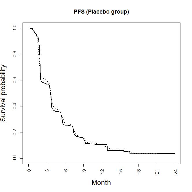
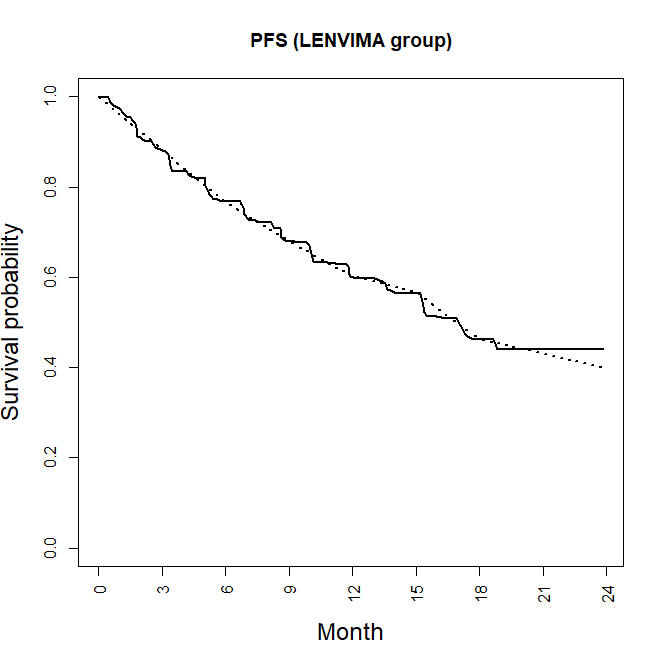
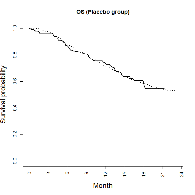
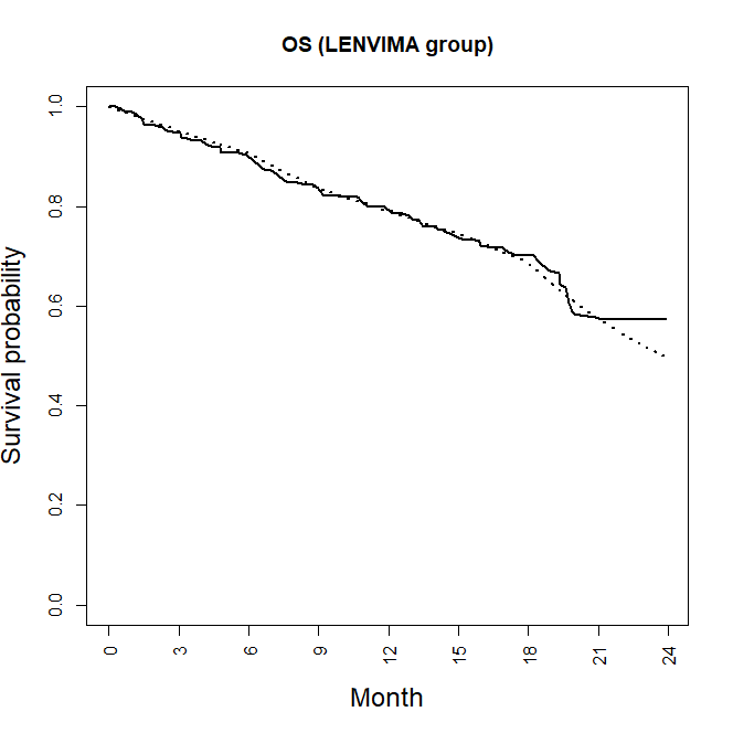
Figure 4: Fitted PFS and OS curves, where the solid lines are re-engineered survival curves from the originally reported K-M curves, and the dotted lines are based on three-state models fit to the re-engineered data.

On August 2014, researchers submitted a new drug application (NDA) seeking approval of lenvatinib (LENVIMA) using data from Study E7080-G000-303 (SELECT) (National Library of Medicine, 2019). LENVIMA is an anti-cancer medication for the treatment of certain types of thyroid cancer. In SELECT, a total of 392 eligible patients were randomly assigned in a 2:1 ratio to the LENVIMA arm and the placebo arm. They were either given LENVIMA at a dose of 24 mg through continuous once-daily oral administration or a matching placebo. Patients received the blinded study drug once daily until any of the following events occurred: confirmed disease progression or withdrawal of consent. Patients in the placebo group, upon having their disease progression confirmed, had the option to request entry into the open-label LENVIMA treatment phase and receive experimental treatment (National Library of Medicine, 2019). After the double-blind phase, patients who received LENVIMA and had not encountered disease progression had the option to request ongoing open-label LENVIMA treatment at the same dosage, as determined by the clinical judgment of the investigator (National Library of Medicine, 2019).

The review document for SELECT provides the Kaplan-Meier (K-M) curves for progression-free survival (PFS), overall survival (OS), and survival after crossover (National Library of Medicine, 2019). Based on these curves, we used the R package IPDfromKM (version 0.1.10 on CRAN) to reconstruct the individual patient data. We then used piecewise exponential models to estimate the hazard rates. We determined the three underlying hazard functions in the three-state models (for treatment and control separately) through trial and error, so that the resulting PFS and OS curves largely matched the reported K-M curves in SELECT. Figure 4 plots the re-engineered survival curves from the originally reported K-M curves (solid lines) vs. the fitted PFS and OS curves (dotted lines).

If we believe that the estimated parameters reflect the underlying truth, then we can design a simulation study based on these parameters. In our simulation study, we assumed that the recruitment was completed in 6 months with a uniform accrual rate. Out of the 392 patients, 261 were randomized to LENVIMA and 131 to placebo (roughly a 2:1 ratio). After randomization, patients were followed to the study cut-off at 24 months or to the censoring time, which was assumed to follow an exponential distribution with monthly hazard rate of $0.004$. Just like the real LENVIMA study, we assumed $83\%$ patients in the placebo group switched to open-label LENVIMA while the rest remained in the placebo group.

Under the settings of our simulation, the HR based on the ITT analysis was $0.859$ favoring the treatment group, and the power was $15.7\%$ based on a two-sided log-rank test with significance level $\alpha=0.05$. However, if placebo patients were not allowed to switch to open-label LENVIMA after disease progression, then the hazard ratio would drop to $0.236$. This is the true treatment effect when crossover is not allowed. The power in this case would be $100\%$. As before, these results were obtained using the R package PWEALL (version 1.4.0 on CRAN).

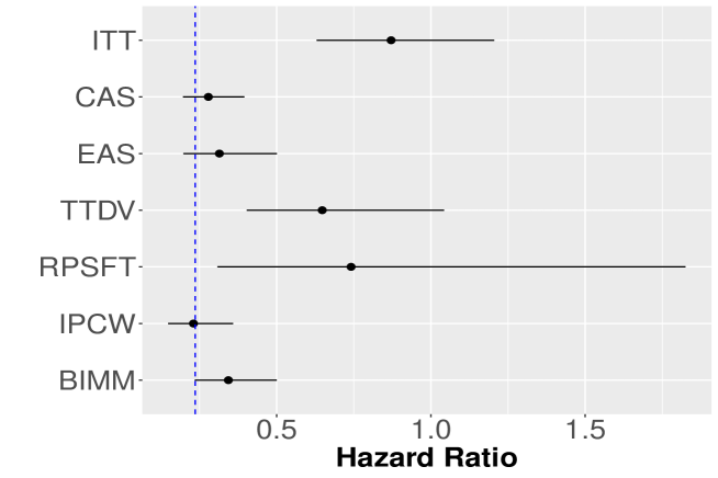
Figure 5: Simulation results from the reverse-engineered LENVIMA data. The dotted blue line denotes true treatment effect when crossover is not allowed.

Our simulation results averaged across 2000 replicates are plotted in Figure 5. A lower estimated treatment effect indicates a larger discrepancy between the LENVIMA and the placebo groups, and thus, suggests greater efficacy of the drug. Figure 5 shows that the estimated HR from the unadjusted ITT analysis deviates significantly from the true HR. After adjusting for crossover, all other methods concluded greater drug effectiveness than that determined by the ITT analysis. Figure 5 shows that the PP methods (CAS and EAS) and the IPCW method performed the best on average, with the lowest magnitude of average bias. In this particular experiment with re-engineered data from the LENVIMA trial, the treatment effect could be best estimated using only data before crossover. On real clinical data, however, researchers should assess the appropriateness of excluding or censoring data after crossover, as well as the implicit assumptions made by the CAS, EAS, or IPCW methods.

5 Discussion

We have proposed the TSM framework which unifies existing and new methods for treatment effect estimation in RCTs with treatment crossover. A number of existing methods (Table 1) are covered in this framework, which allows delineation of these methods in terms of underlying assumptions and limitations. The TSM framework also allows for the creation of new methods that incorporate diverse assumptions tailored to specific scenarios, thus enhancing its applicability in RCTs. A new imputation method for modeling the counterfactual survival time under treatment crossover was proposed and illustrated under this framework. By adopting a statistical perspective, our work complements and augments the comparative numerical studies of different methods by Morden et al. (2011) and Latimer et al. (2018).

Modeling the data after treatment crossover to estimate the true treatment effect is essentially an imputation problem. In general, post-crossover data are biased, and different methods treat the biased data in different ways. The best choice of imputation method(s) depends on the assumptions about the types of crossover and the nature of the data. This is especially the case when $100\%$ of patients in the control group cross over to the experimental treatment, and thus, the true treatment effect is not identifiable without more stringent assumptions. Apart from the Markov (6) and semi-Markov (7) crossover assumptions, other implicit assumptions for each method also need to be carefully assessed (e.g. the assumption of a constant treatment effect in TTDV and RPSFT, the assumption of conditional independence of time-to-event and time-to-crossover given covariates in IPCW, etc.). It is important for researchers to be transparent about potential sources of bias inherent in their assumptions and properly report the limitations of their approaches.

References

- (1)
- Arnold & Ercumen (2016) Arnold, B. F. & Ercumen, A. (2016), ‘Negative control outcomes: A tool to detect bias in randomized trials’, JAMA 316(24), 2597–2598.
- Austin (2011) Austin, P. C. (2011), ‘An introduction to propensity score methods for reducing the effects of confounding in observational studies’, Multivariate Behavioral Research 46(3), 399–424.
- Bennett (2018) Bennett, I. (2018), ‘Accounting for uncertainty in decision analytic models using rank preserving structural failure time modeling: Application to parametric survival models’, Value in Health 21(1), 105–109.
- Brody (2016) Brody, T. (2016), Chapter 8 - Intent-to-treat analysis versus per protocol analysis, in T. Brody, ed., ‘Clinical Trials (Second Edition)’, Academic Press, Boston, pp. 173–201.
- Carpenter et al. (2017) Carpenter, B., Gelman, A., Hoffman, M. D., Lee, D., Goodrich, B., Betancourt, M., Brubaker, M., Guo, J., Li, P. & Riddell, A. (2017), ‘Stan: A probabilistic programming language’, Journal of Statistical Software 76(1), 1–32.
- Cox (1972) Cox, D. R. (1972), ‘Regression models and life-tables’, Journal of the Royal Statistical Society. Series B (Methodological) 34(2), 187–220.
- Curtis et al. (2007) Curtis, L. H., Hammill, B. G., Eisenstein, E. L., Kramer, J. M. & Anstrom, K. J. (2007), ‘Using inverse probability-weighted estimators in comparative effectiveness analyses with observational databases’, Medical Care 45, S103–S107.
- Dancey et al. (2009) Dancey, J., Dodd, L., Ford, R., Kaplan, R., Mooney, M., Rubinstein, L., Schwartz, L., Shankar, L. & Therasse, P. (2009), ‘Recommendations for the assessment of progression in randomised cancer treatment trials’, European Journal of Cancer 45(2), 281–289.
- Daugherty et al. (2008) Daugherty, C. K., Ratain, M. J., Emanuel, E. J., Farrell, A. T. & Schilsky, R. L. (2008), ‘Ethical, scientific, and regulatory perspectives regarding the use of placebos in cancer clinical trials’, Journal of Clinical Oncology 26(8), 1371–1378.
- Glidden et al. (2020) Glidden, D. V., Stirrup, O. T. & Dunn, D. T. (2020), ‘A Bayesian averted infection framework for PrEP trials with low numbers of HIV infections: application to the results of the DISCOVER trial’, The Lancet HIV 7(11), e791–e796.
- Ibrahim et al. (2001) Ibrahim, J. G., Chen, M.-H. & Sinha, D. (2001), Bayesian Survival Analysis, Springer-Verlag, New York, NY.
- Ishak et al. (2011) Ishak, K. J., Caro, J. J., Drayson, M. T., Dimopoulos, M., Weber, D., Augustson, B., Child, J. A., Knight, R., Iqbal, G., Dunn, J., Shearer, A. & Morgan, G. (2011), ‘Adjusting for patient crossover in clinical trials using external data: A case study of lenalidomide for advanced multiple myeloma’, Value in Health 14(5), 672–678.
- Ishak et al. (2014) Ishak, K. J., Proskorovsky, I., Korytowsky, B., Sandin, R., Faivre, S. & Valle, J. (2014), ‘Methods for adjusting for bias due to crossover in oncology trials’, Pharmacoeconomics 32(6), 533–546.
- Jönsson et al. (2014) Jönsson, L., Sandin, R., Ekman, M., Ramsberg, J., Charbonneau, C., Huang, X., Jönsson, B., Weinstein, M. C. & Drummond, M. (2014), ‘Analyzing overall survival in randomized controlled trials with crossover and implications for economic evaluation’, Value in Health 17(6), 707–713.
- Kahan & Morris (2013) Kahan, B. C. & Morris, T. P. (2013), ‘Adjusting for multiple prognostic factors in the analysis of randomised trials’, BMC Medical Research Methodology 13(99).
- Latimer et al. (2014) Latimer, N. R., Abrams, K. R., Lambert, P. C., Crowther, M. J., Wailoo, A. J., Morden, J. P., Akehurst, R. L. & Campbell, M. J. (2014), ‘Adjusting survival time estimates to account for treatment switching in randomized controlled trials—an economic evaluation context: Methods, limitations, and recommendations’, Medical Decision Making 34(3), 387–402.
- Latimer et al. (2018) Latimer, N. R., Abrams, K. R., Lambert, P. C., Morden, J. P. & Crowther, M. J. (2018), ‘Assessing methods for dealing with treatment switching in clinical trials: A follow-up simulation study’, Statistical Methods in Medical Research 27(3), 765 – 784.
- Luo et al. (2019) Luo, X., Mao, X., Chen, X., Qiu, J., Bai, S. & Quan, H. (2019), ‘Design and monitoring of survival trials in complex scenarios’, Statistics in Medicine 38(2), 192–209.
- McKeever (2021) McKeever, L. (2021), ‘Overview of study designs: A deep dive into research quality assessment’, Nutrition in Clinical Practice 36(3), 569–585.
- Morden et al. (2011) Morden, J. P., Lambert, P. C., Latimer, N., Abrams, K. R. & Wailoo, A. J. (2011), ‘Assessing methods for dealing with treatment switching in randomised controlled trials: A simulation study’, BMC Medical Research Methodology 11(4).
- National Library of Medicine (2019) National Library of Medicine (2019), ‘A multicenter, randomized, double-blind, placebo-controlled, trial of Lenvatinib (E7080) in 131I-refractory differentiated thyroid cancer (DTC) (SELECT)’, https://clinicaltrials.gov/study/NCT01321554. Accessed: 14 November 2023.
- Paganoni et al. (2022) Paganoni, S., Watkins, C., Cawson, M., Hendrix, S., Dickson, S. P., Knowlton, N., Timmons, J., Manuel, M. & Cudkowicz, M. (2022), ‘Survival analyses from the CENTAUR trial in amyotrophic lateral sclerosis: Evaluating the impact of treatment crossover on outcomes’, Muscle & Nerve 66(2), 136–141.
- Robins & Finkelstein (2000) Robins, J. M. & Finkelstein, D. M. (2000), ‘Correcting for noncompliance and dependent censoring in an AIDS clinical trial with inverse probability of censoring weighted (IPCW) log-rank tests’, Biometrics 56(3), 779–788.
- Robins & Tsiatis (1991a) Robins, J. M. & Tsiatis, A. A. (1991a), ‘Correcting for non-compliance in randomized trials using rank preserving structural failure time models’, Communications in Statistics - Theory and Methods 20(8), 2609–2631.
- Robins & Tsiatis (1991b) Robins, J. M. & Tsiatis, A. A. (1991b), ‘Correcting for non-compliance in randomized trials using rank preserving structural failure time models’, Communications in Statistics - Theory and Methods 20(8), 2609–2631.
- Simon & Chinchilli (2007) Simon, L. J. & Chinchilli, V. M. (2007), ‘A matched crossover design for clinical trials’, Contemporary Clinical Trials 28(5), 638–646.
- Watkins et al. (2013) Watkins, C., Huang, X., Latimer, N., Tang, Y. & Wright, E. (2013), ‘Adjusting overall survival for treatment switches: Commonly used methods and practical application’, Pharmaceutical Statistics 12(6), 348–357.
- White (2005) White, I. R. (2005), ‘Uses and limitations of randomization-based efficacy estimators’, Statistical Methods in Medical Research 14(4), 327–347.
- White et al. (1999) White, I. R., Babiker, A. G., Walker, S. & Darbyshire, J. H. (1999), ‘Randomization-based methods for correcting for treatment changes: Examples from the Concorde trial’, Statistics in Medicine 18(19), 2617–2634.
- White et al. (1997) White, I. R., Walker, S., Babiker, A. G. & Darbyshire, J. H. (1997), ‘Impact of treatment changes on the interpretation of the Concorde trial’, AIDS 11(8), 999–1006.