Classical certification of quantum computation under the dimension assumption

Abstract

Certification of quantum computing components can be crucial for quantum hardware improvements and the calibration of quantum algorithms. In this work, we propose an efficient method for certifying single-qubit quantum computation in a black-box scenario under the dimension assumption. The method is based on testing deterministic outcomes of quantum computation for predetermined gate sequences. Quantum gates are certified based on input-output correlations, with no auxiliary systems required. We show that a single-qubit universal gate set can be certified and analyze in detail certification of the S gate, for which the required sample complexity grows as $\operatorname{\mathrm{O}}(\varepsilon^{-1})$ with respect to the average gate infidelity $\varepsilon$. Our approach takes a first step in bridging the gap between strong notions of certification from self-testing and practically highly relevant approaches from quantum system characterization.

I Introduction

High-quality quantum gate implementations are crucial for nearly every quantum information processing task and, in particular, are the central components in most quantum computing platforms. Practical challenges arise as state preparations, gates and measurements are inherently noisy, and their characterization is a complicated but vital task. Extensive efforts have been invested in characterizing these elements, giving rise to the field of quantum system characterization (see Refs. [1, 2] for reviews). Through these characterization protocols, the level of noise can be determined, and the most significant errors identified, fostering trust in the reliability of quantum computing components. Such information can be crucial for improving the quantum hardware, tailoring and calibrating the software to perform well under the noise of a given platform [3].

A particular challenge of determining noise properties of any gate implementation are posed by unavoidable state preparation and measurement (SPAM) errors. They are a limiting factor in standard quantum process tomography [4, 5] and direct certification methods [6, 7, 8]. Two broad families of characterization methods have been developed to address this challenge: gate set tomography (GST) [9, 10] and randomized benchmarking (RB) [11, 12, 13, 14, 15, 16, 17] with its many variants (see Refs. [17, 18] for a recent overview). In both types of protocols, gate errors are amplified by running longer gate sequences in order to measure them in a way that is robust against SPAM errors. GST aims to fully reconstruct the quantum gates in a self-consistent fashion and is, hence, intrinsically non-scalable, while RB is more scalable and, in turn, gives very coarse grained information on the gate implementations such as a single decay parameter.

Crucially, both methods only establish the existence of a quantum model consistent with the data, and there is currently no method in the quantum characterization literature that is both resilient to SPAM errors and capable of certifying a quantum model uniquely. GST comes closest to this aim, but the explicit form of the non-uniqueness of the estimated model, i.e., the gauge-freedom, is not well-studied [19], and GST is not supported by full guarantees. Moreover, its measurement effort is daunting so that it is not a convenient tool for certification. RB is designed to be scalable but requires even more assumptions: the gate implementations have to be already close to the targeted ones and only then the closeness can be quantified in terms of a decay parameter [17, 18].

Currently, it is unclear how one can confirm that such model assumptions are met and the stability of existing protocols against potential violations remains uncertain. In this context, ideally, one would like to uniquely certify quantum operations, in particular implementations of quantum gates, device-independently, i.e., in a black-box scenario without any assumptions. Such a strong notion of certification is known as self-testing [20], a concept first introduced for the certification of entangled states and incompatible measurements in the Bell experiment [21].

However, achieving this strong notion of assumption-free certification necessitates two space-like separated quantum devices. This requirement is experimentally challenging and misaligns with the practically motivated setup with a quantum server and classical users, which is inherent to foreseeable quantum computation. An alternative avenue of research [22, 23], designed for certifying a single quantum computer in a black-box scenario, relies on computational assumptions, providing the potential for classical certification of quantum computers. Nevertheless, this method is currently out of reach for quantum hardware due to its demanding requirements on the number of qubits and the fidelity of implemented gates [24].

In this work, our goal is to achieve SPAM error-free certification of a quantum computer’s correct functioning, without requiring physical access to it. This investigation is particularly relevant in a practical server-user configuration: a classical user via classical channel transmits gate sequences to the server, which then implements them and returns the measurement outcomes. Since achieving this goal without any assumptions is impossible, we propose an efficient method for certifying single-qubit quantum computation in a black-box scenario under a minimal assumption, the dimension assumption. Moreover, since we assume that no part of the quantum apparatus, such as the measurement device, is characterized prior to the test, certification is only possible up to the degrees of freedom inherent to quantum mechanics, unitary or anti-unitary transformations (a unitary followed by a complex conjugation) [25, 10, 26, 27, 28, 29, 19]. It is important to note that this is the absolute minimum degree of freedom that cannot be excluded in black-box tests, as it corresponds to the simultaneous change of bases. A more general gauge freedom is sometimes considered in the GST literature [9, 30, 19].

Our method is based on a very intuitive idea of testing deterministic measurement outcomes for quantum gate sequences that can be resolved efficiently classically. Examples may include a gate sequence that composes into the identity gate or simply a zero-length sequence, for which the system is measured directly after the state preparation. Certification is then enabled by invoking the dimension assumption, in our case one qubit, which limits the probability that a noisy quantum computer will produce the correct result. For certification of quantum gates, only the input-output correlations are used and no entanglement with an auxiliary system is required. Here, we prove that a universal gate set for single qubit quantum operations can be certified within our framework, and analyze in detail certification of a single phase shift gate, for which the required sample complexity, measured in terms of the number of individual runs of the experiment or the number of tested system copies [2], grows as $\operatorname{\mathrm{O}}(\varepsilon^{-1})$ with respect to the average gate infidelity $\varepsilon$.

The rest of the paper is organized as follows. In Section II, we explain the experimental setup, outline the assumptions, and describe the protocol. In Section III, we present our results on certification of single-qubit quantum operations, with the main contributions stated as Theorem 3, Corollary 4, and Theorem 5. Technical details supporting the main claims of the paper are left to the appendix.

II Setup and protocol

Figure 1: Scenario of the certification test. A system is prepared in state $\rho$ and undergoes a series of transformations, $\Lambda_{x_{1}}$, $\Lambda_{x_{2}}$, …, $\Lambda_{x_{m}}$, specified by classical instructions $\{x_{i}\}_{i=1}^{m}$ from a fixed set, after which it is measured in a fixed basis, producing outcome $a$. The sequences $\mathbf{x}=x_{1}x_{2}\dots x_{m}$ of varied length $m$ are chosen at random from the predetermined set $\mathcal{X}$.

The experimental setup that we consider is common to many established certification methods, such as RB [17] and GST [9]. The setup, or scenario as it would be called in the self-testing literature, is shown schematically in Fig. 1. A quantum system is prepared in some initial state, after which a sequence of quantum gates is applied to it, and it is finally measured in some fixed basis. For each gate in a given sequence, a label, chosen from some finite set $X$, is communicated to the quantum computer. The certification protocol relies on a particular finite subset of sequences $\mathcal{X}\subset X^{\ast}$, which are determined before the protocol begins. In a single repetition of the protocol, a random string $\mathbf{x}\coloneqq x_{1}x_{2}\dots x_{m}$ is selected from $\mathcal{X}$, and after the quantum computer implements the corresponding computation, the outcome $a\in A$ of the measurement is read out, where $A$ is the set of all possible outcomes. The certification protocol decides to proceed or abort, depending on the deterministic outcome $a_{\mathbf{x}}$, corresponding to the ideal implementation of the target quantum computation. The length $m$ of different sequences $\mathbf{x}\in\mathcal{X}$ can be different, and, in particular, be zero, which we denote by the empty string $\epsilon$, and by which we mean that the system is measured directly after the state preparation.

Given our emphasis on the minimal nature of the assumptions in our method, we explicitly enumerate them below.

• The dimension assumption. We assume that the underlying quantum model is mathematically described by a density operator $\rho$, a set of completely positive trace preserving (CPTP) maps $\{\Lambda_{x}\}_{x\in X}$, and a positive operator-valued measure (POVM) $(M_{a})_{a\in A}$, all defined over a Hilbert space of a specified dimension.

• Context independence. We assume that in each repetition of our protocol, for each label $x$ the quantum computer implements the corresponding quantum channel $\Lambda_{x}$ in the same way, irrespective of the sequence $\mathbf{x}$ in which the gate $x$ appears or the order in which it appears in this sequence. In the certification literature, this assumption is often referred to as existence of the single-shot implementation function.

• Independence of repetitions. We assume that quantum models in different repetitions of the protocol are independent. Note, that we do not need the assumption that quantum models in different repetitions of the protocol are identical.

Other minor assumptions include error-free functioning of the classical part of the quantum computer, such as control circuits, and our ability to randomly select the gate sequences. Importantly, our protocol is robust against deviations from the target distribution $\mu(\mathbf{x})$ according to which we sample the random sequences $\mathbf{x}$ from $\mathcal{X}$.

We are ready to present our protocol. We give a general formulation for a given set of gates $X$, with an important property that among all possible sequences $X^{\ast}$, there are such $\mathbf{x}$, for which we can predict the deterministic outcome $a_{\mathbf{x}}$, which a noiseless quantum computer should output.

Protocol 1 Certification of single-qubit quantum computation under the dimension assumption

  Set $N$ – the number of repetitions, and $\mathcal{X}$ – the set of gate sequences $\mathbf{x}$, each with the corresponding deterministic outcome $a_{\mathbf{x}}$;

  for $i\in[N]$ do

     sample $\mathbf{x}$ from $\mathcal{X}$, according to $\mu(\mathbf{x})$;

     execute a quantum circuit consisting of the state preparation, the sequence $\mathbf{x}$ of gates, and the measurement, record the outcome $a$;

     if $a\neq a_{\mathbf{x}}$ then

        output ‘‘reject’’ and end the protocol;

  output ‘‘accept’’.

Protocol 1 has a simple form of an $\varepsilon$-certification test, which is common in certification literature [2]. The basic idea is that if we repeat Protocol 1 sufficiently many times for different sequences $\mathbf{x}$ and obtain the correct outcome $a_{\mathbf{x}}$ in all these repetitions, then we can obtain a certain level of confidence, typically denoted by $1-\delta$, that our quantum computer implements a quantum model correctly. We define more precisely below what we mean by the latter, building on similar definitions in the self-testing literature [28]. First, we specify what we mean by a quantum model in the context of single-qubit quantum computation.

Definition 1.

A quantum model is a $3$-tuple $(\rho,\{\Lambda_{x}\}_{x\in X},(M_{a})_{a\in A})$, consisting of a quantum state $\rho$, prepared at the beginning of the quantum computation, a set of quantum channels (gates) $\{\Lambda_{x}\}_{x\in X}$, from which a quantum circuit is composed, and a POVM $(M_{a})_{a\in A}$, measured at the end of the computation.

For a quantum model involving only unitary quantum channels, we use the corresponding unitary operators in the definition of the model. Since we do not assume any part of the quantum computer to be characterized, and rely only on the classical data in our certification, any two quantum models which are equivalent up to the choice of a reference frame will produce the same statistics, and we will not be able to distinguish between them. At the same time, we would like to exclude any other quantum model, which is formalized by the following definition.

Definition 2.

For a target quantum model, $(\rho,\{U_{x}\}_{x\in X},(M_{a})_{a\in A})$ with unitary channels, we say that a quantum computer implements it correctly, if there exists a unitary operator $U$ (with a possible complex conjugation ^(∗)), such that the implemented quantum model $(\tilde{\rho},\{\tilde{\Lambda}_{x}\}_{x\in X},(\tilde{M}_{a})_{a\in A})$ satisfies

$$\begin{split}\tilde{\rho}&=U\rho^{(\ast)}U^{\dagger},\\ \tilde{\Lambda}_{x}({\,\cdot\,})&=UU_{x}^{(\ast)}U^{\dagger}({\,\cdot\,})U{U_{x}^{\dagger}}^{(\ast)}U^{\dagger},\quad\forall x\in X,\\ \tilde{M}_{a}&=UM_{a}^{(\ast)}U^{\dagger},\quad\forall a\in A.\end{split}$$ (1)

Following the terminology of the self-testing literature [20], we say that the target outcomes $a_{\mathbf{x}}$ self-test a quantum model, if from the fact that the observed outcomes correspond to $a_{\mathbf{x}}$, we can infer that the quantum computer implements the quantum model correctly, in the sense of Definition 2. Moreover, we say that the self-test is robust, if for small deviations in the outcomes, the target and the implemented models are close in some distance.

Following the terminology of the certification literature [2], we say that Protocol 1 is an $\varepsilon$-certification test for a target quantum model with respect to appropriately chosen distances, if the protocol is complete and sound. Completeness means that the target quantum model will be accepted by the protocol with high probability. Soundness, in light of Definition 2, means that any quantum model for which there is no unitary or unitary and transposition, which brings it $\varepsilon$-close to the target model with respect to the chosen distances, will be rejected by the protocol with high probability.

In the next section, we prove that Protocol 1 is an $\varepsilon$-certification test for a quantum model $(|+\kern 0.6458pt\rangle\langle\kern 0.6458pt\mathopen{}+|,\{\mathrm{S},\mathrm{S}^{\dagger}\},(|\pm\kern 0.6458pt\rangle\langle\kern 0.6458pt\mathopen{}\pm|)_{\pm})$, for which we first prove a robust self-testing result. Then, we prove a self-testing result for a quantum model with an additional $\mathrm{H}$ gate and the square root of the $\mathrm{S}$ gate, i.e., the model $(|+\kern 0.6458pt\rangle\langle\kern 0.6458pt\mathopen{}+|,\{\mathrm{S},\mathrm{S}^{\dagger},\mathrm{H},\sqrt{\mathrm{S}}\},(|\pm\kern 0.6458pt\rangle\langle\kern 0.6458pt\mathopen{}\pm|)_{\pm})$, which shows that a single-qubit universal gate set can be certified with Protocol 1.

III Certification of single-qubit quantum models

III.1 Self-testing and certification of the S gate

We explain in detail certification of the $\mathrm{S}$ gate, or more precisely, the set $\{\mathrm{S},\mathrm{S}^{\dagger}\}$, the $\mathrm{S}$ gate and its inverse. We set $X=\{\mathrm{s},{\mathrm{s}^{\scaleobj{.8}{{-1}}}}\}$ for the classical instructions given to a quantum computer which specify whether it should implement the $\mathrm{S}$ or its inverse, respectively.

Surprisingly, it is sufficient to consider the following set of strings in Protocol 1

$$\mathcal{X}=\{\epsilon,\mathrm{s}\mathrm{s},\mathrm{s}{\mathrm{s}^{\scaleobj{.8}{{-1}}}},{\mathrm{s}^{\scaleobj{.8}{{-1}}}}\mathrm{s},{\mathrm{s}^{\scaleobj{.8}{{-1}}}}{\mathrm{s}^{\scaleobj{.8}{{-1}}}}\},$$ (2)

where $\epsilon$ denotes the empty string. Next, we set $A=\{+,-\}$, and for the sequences in Eq. 2, the deterministic outcomes corresponding to the target model are the following

$$a_{\mathbf{x}}=\left\{\begin{array}[]{ c l }+&\quad\textrm{for }\mathbf{x}\in\{\epsilon,\mathrm{s}{\mathrm{s}^{\scaleobj{.8}{{-1}}}},{\mathrm{s}^{\scaleobj{.8}{{-1}}}}\mathrm{s}\},\\ -&\quad\textrm{for }\mathbf{x}\in\{\mathrm{s}\mathrm{s},{\mathrm{s}^{\scaleobj{.8}{{-1}}}}{\mathrm{s}^{\scaleobj{.8}{{-1}}}}\}.\end{array}\right.$$ (3)

It can be easily seen that preparing the qubit system in the initial state $\rho=|+\kern 0.6458pt\rangle\langle\kern 0.6458pt\mathopen{}+|$ and measuring it in the X-basis, satisfies the criterion in Eq. 3. Therefore, in case of noiseless implementation of the state preparation, the gates $\{\mathrm{S},\mathrm{S}^{\dagger}\}$, and the measurement, Protocol 1 always accepts. In other words, Protocol 1 is complete for certification of the $\mathrm{S}$ gate, with $\mathcal{X}$ and $\{a_{\mathbf{x}}\}_{\mathbf{x}\in\mathcal{X}}$ specified by Eq. 2 and Eq. 3, respectively.

Proving the soundness of the protocol is much less straightforward. To achieve this, we first state and prove the following self-testing result.

Theorem 3.

For a single-qubit quantum model $(\tilde{\rho},\{\tilde{\Lambda}_{\mathrm{s}},\tilde{\Lambda}_{\mathrm{s}^{\scaleobj{.8}{{-1}}}}\},(\tilde{M}_{+},\tilde{M}_{-}))$, which passes a single repetition of Protocol 1 with probability at least $1-\varepsilon$, for $\mathcal{X}$ and $a_{\mathbf{x}}$ specified in Eq. 2 and Eq. 3, respectively, and for the uniform $\mu(\mathbf{x})$, there exists a unitary $U\in\operatorname{U}(2)$, such that

$$\begin{split}\mathrm{F}_{\mathrm{avg}}(\tilde{\Lambda}_{\mathrm{s}},U\mathrm{S}U^{\dagger})&\geq 1-\operatorname{\mathrm{O}}(\varepsilon),\\ \mathrm{F}_{\mathrm{avg}}(\tilde{\Lambda}_{\mathrm{s}^{\scaleobj{.8}{{-1}}}},U\mathrm{S}^{\dagger}U^{\dagger})&\geq 1-\operatorname{\mathrm{O}}(\varepsilon),\\ \operatorname{Tr}[\tilde{\rho}U|+\kern 0.6458pt\rangle\langle\kern 0.6458pt\mathopen{}+|U^{\dagger}]&\geq 1-\frac{15}{2}\varepsilon,\\ \left\lVert\tilde{M}_{+}-U|+\kern 0.6458pt\rangle\langle\kern 0.6458pt\mathopen{}+|U^{\dagger}\right\rVert_{\infty}&\leq\frac{5}{2}\varepsilon,\end{split}$$ (4)

where $\mathrm{F}_{\mathrm{avg}}$ is the average gate fidelity.

For the definition of the average gate fidelity, we refer the reader to Ref. [2]. In the case of unitary channels, we use the respective operators as the argument of the fidelity function for simplicity of notation. Below, we give a sketch of the proof, and the full proof can be found in Appendix A.

Proof sketch.

The conclusions of the theorem follow from the condition $\mathbb{P}[\text{{{``pass''}}}]\geq 1-\varepsilon$ and the dimension assumption. As a first step, we show that for small $\varepsilon$, the measurement effects $\tilde{M}_{+}$ and $\tilde{M}_{-}$ are close to being rank-1 projectors, which we denote as $\psi$ and $\psi^{\perp}$. Next, we show that the POVMs which one obtains by applying the adjoint maps $\tilde{\Lambda}_{\mathrm{s}}^{\dagger}$ and $\tilde{\Lambda}_{\mathrm{s}^{\scaleobj{.8}{{-1}}}}^{\dagger}$ to $\psi$ and $\psi^{\perp}$ are also close to be projective for small $\varepsilon$. We denote the corresponding projectors by $\phi$ and $\phi^{\perp}$. Importantly, we find that $\tilde{\Lambda}_{\mathrm{s}}^{\dagger}(\psi)\approx\phi$ and $\tilde{\Lambda}_{\mathrm{s}^{\scaleobj{.8}{{-1}}}}^{\dagger}(\psi)\approx\phi^{\perp}$, and since the adjoint maps of channels are unital, also $\tilde{\Lambda}_{\mathrm{s}}^{\dagger}(\psi^{\perp})\approx\phi^{\perp}$ and $\tilde{\Lambda}_{\mathrm{s}^{\scaleobj{.8}{{-1}}}}^{\dagger}(\psi^{\perp})\approx\phi$. Next, we obtain a partial characterization of the Choi-Jamiołkowski [31, 32] state of the channel $\tilde{\Lambda}_{\mathrm{s}}$ in the basis of $\psi$ and $\phi$, with the leading terms corresponding to the subspace spanned by $|\psi\rangle|\phi\rangle$ and $|\psi^{\perp}\rangle|\phi^{\perp}\rangle$. Then, we show that $\tilde{\Lambda}_{\mathrm{s}}$ is close to being a unitary channel, for which we use the conditions $\tilde{\rho}\approx\psi$ and $\tilde{\Lambda}_{\mathrm{s}}(\tilde{\rho})\approx\phi^{\perp}$. Finally, we find a suitable gauge unitary $U\in\operatorname{U}(2)$ for which the condition for $\tilde{\Lambda}_{\mathrm{s}}$ in Eq. 4 is satisfied. Because we obtain characterization of $\tilde{\Lambda}_{\mathrm{s}}$ and $\tilde{\Lambda}_{\mathrm{s}^{\scaleobj{.8}{{-1}}}}$ in the same basis, the proof also easily extends to the channel $\tilde{\Lambda}_{\mathrm{s}^{\scaleobj{.8}{{-1}}}}$. The bounds for the state and the measurement in Eq. 4 with the chosen unitary are also immediate. ∎

Interestingly, in the ideal case of $\varepsilon=0$, the self-testing argument can also be made for the set of gate sequences without ${\mathrm{s}^{\scaleobj{.8}{{-1}}}}{\mathrm{s}^{\scaleobj{.8}{{-1}}}}$, or without $\mathrm{s}\mathrm{s}$. Moreover, the effect that the sampling distribution $\mu(\mathbf{x})$ plays in Theorem 3 is purely in determining the constants in front of $\varepsilon$, with the only requirement that each sequence in $\mathcal{X}$ is chosen with some nonzero probability.

We can use the known relation that connects the average gate fidelity and the diamond distance for an arbitrary qubit channel $\tilde{\Lambda}$ and a unitary channel $\Lambda$ [2],

$$\left\lVert\tilde{\Lambda}-\Lambda\right\rVert_{\diamond}\leq 2\sqrt{6}\sqrt{1-\mathrm{F}_{\mathrm{avg}}(\tilde{\Lambda},\Lambda)},$$ (5)

to reformulate Theorem 3 for the diamond distance with an upper bound of $\operatorname{\mathrm{O}}(\sqrt{\varepsilon})$. It is also clear, that even though we state Theorem 3 for the target quantum model consisting of the $\mathrm{S}$ gate, initial state $|+\kern 0.6458pt\rangle\langle\kern 0.6458pt\mathopen{}+|$ and the $\mathrm{X}$-basis measurement, the same exact result holds for any target quantum model which is unitary equivalent to it, e.g., $(|0\kern 0.6458pt\rangle\langle\kern 0.6458pt\mathopen{}0|,\{\sqrt{\mathrm{X}},\sqrt{\mathrm{X}}^{\dagger}\},(|0\kern 0.6458pt\rangle\langle\kern 0.6458pt\mathopen{}0|,|1\kern 0.6458pt\rangle\langle\kern 0.6458pt\mathopen{}1|))$.

Next, using Theorem 3, we show that Protocol 1 is sound for certification of the model $(|+\kern 0.6458pt\rangle\langle\kern 0.6458pt\mathopen{}+|,\{\mathrm{S},\mathrm{S}^{\dagger}\},(|\pm\kern 0.6458pt\rangle\langle\kern 0.6458pt\mathopen{}\pm|)_{\pm})$, as stated by the following corollary. This corollary is the main practical result of the current paper.

Corollary 4.

Protocol 1 with $\mathcal{X}$ and $a_{\mathbf{x}}$ specified in Eq. 2 and Eq. 3, respectively, and the uniform $\mu(\mathbf{x})$ is an $\varepsilon$-certification test for the $\mathrm{S}$ gate and its inverse with respect to the average gate fidelity, as well as initial state $|+\kern 0.6458pt\rangle\langle\kern 0.6458pt\mathopen{}+|$ and measurement $(|+\kern 0.6458pt\rangle\langle\kern 0.6458pt\mathopen{}+|,|-\kern 0.6458pt\rangle\langle\kern 0.6458pt\mathopen{}-|)$ with respect to fidelity and spectral norm, from $N$ independent samples for $N\geq N_{0}$ with

$$N_{0}=\operatorname{\mathrm{O}}(\varepsilon^{-1})\ln(\delta^{-1}),$$ (6)

with confidence at least $1-\delta$. Moreover, Protocol 1 accepts the target model $(|+\kern 0.6458pt\rangle\langle\kern 0.6458pt\mathopen{}+|,\{\mathrm{S},\mathrm{S}^{\dagger}\},(|\pm\kern 0.6458pt\rangle\langle\kern 0.6458pt\mathopen{}\pm|)_{\pm})$ with probability $1$.

The lower bound of $N_{0}$ in Corollary 4 should be interpreted as a sufficient number of repetitions of Protocol 1 to reach the target confidence level $1-\delta$.

Proof.

We can invert the statement of Theorem 3, and obtain that for a noisy quantum model, for which there does not exist a unitary $U\in\operatorname{U}(2)$, satisfying Eq. 4, the probability of passing a single repetition of Protocol 1 is $\mathbb{P}[\text{{{``pass''}}}]\leq 1-\varepsilon$. If we take $N$ independent copies of such noisy $\tilde{\Lambda}_{\mathrm{s}}$, $\tilde{\Lambda}_{\mathrm{s}^{\scaleobj{.8}{{-1}}}}$, as well as $\tilde{\rho}$ and $(\tilde{M}_{+},\tilde{M}_{-})$, the probability of Protocol 1 accepting them is

$$\mathbb{P}[\text{{{``accept''}}}]\leq(1-\varepsilon)^{N}.$$ (7)

For the target confidence level $1-\delta$, the acceptance probability in Eq. 7 should be upper-bounded by $\delta$, which leads to a lower bound on $N$,

$$N\geq\frac{\ln(\delta^{-1})}{\ln\frac{1}{1-\varepsilon}}.$$ (8)

Approximating the logarithm function for $\frac{1}{1-\varepsilon}$, and rescaling $\varepsilon$ such that the lower bounds on the average gate fidelity in Eq. 4 are exactly $1-\varepsilon$, leads to the sample complexity stated in Eq. 6. ∎

As Corollary 4 demonstrates, our method for certification of quantum gates is as efficient as the direct certification of quantum processes [6], which requires trust in state preparations and measurements (and hence is not SPAM robust) and also requires an auxiliary system to prepare the Choi-Jamiołkowski state of the process. The only price to pay is a possibly larger constant factor, which we numerically estimate for the uniform $\mu(\mathbf{x})$ in what follows.

III.2 Numerical investigations

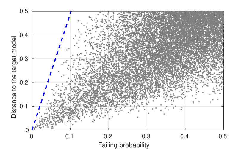
Figure 2: Approximately $10^{4}$ random quantum models are represented by the dots on the plot, with $x$-axis corresponding to the probability that a quantum model fails a single repetition of Protocol 1, and $y$-axis corresponding to the distance to the target model with the unitary gauge chosen as in the proof of Theorem 3. The dashed line correspond to the worst linear coefficient among $10^{7}$ sampled models, with the slope of $\approx 4.9$.

In this subsection, we supplement our theoretical results of Theorem 3 and Corollary 4 by numerical investigations. This also allows us to estimate the coefficients of the linear scaling in Theorem 3, which then translates to an explicit formula for the sample complexity in Corollary 4. The results of our numerical investigations are shown in Fig. 2.

For each randomly generated quantum model $(\tilde{\rho},\{\tilde{\Lambda}_{\mathrm{s}},\tilde{\Lambda}_{\mathrm{s}^{\scaleobj{.8}{{-1}}}}\},(\tilde{M}_{+},\tilde{M}_{-}))$, we calculate the probability of it failing a single repetition of the protocol, which corresponds to $\varepsilon$ in the statement of Theorem 3. We then apply a unitary to the target model, which explicitly depends on the noisy random model, as described in the proof of Theorem 3, and calculate the distance between the noisy model and the target model. For the latter, we take the maximum among the respective distances for the quantum state (infidelity), channels (average gate infidelity), and the measurement (spectral norm) in Eq. 4.

To generate random noisy quantum models, we apply independent unitary noise to the target state, channels, and the measurement, i.e., we take $\tilde{\rho}=U_{1}|+\kern 0.6458pt\rangle\langle\kern 0.6458pt\mathopen{}+|U_{1}^{\dagger}$, $\tilde{\Lambda}_{\mathrm{s}}({\,\cdot\,})=U_{2}\mathrm{S}({\,\cdot\,})\mathrm{S}^{\dagger}U^{\dagger}_{2}$, $\tilde{\Lambda}_{\mathrm{s}^{\scaleobj{.8}{{-1}}}}({\,\cdot\,})=U_{3}\mathrm{S}^{\dagger}({\,\cdot\,})\mathrm{S}U^{\dagger}_{3}$, $\tilde{M}_{+}=U_{4}|+\kern 0.6458pt\rangle\langle\kern 0.6458pt\mathopen{}+|U^{\dagger}_{4}$, and $\tilde{M}_{-}=\mathds{1}-\tilde{M}_{+}$. Sampling Haar-random unitaries $U_{1},U_{2},U_{3}$, and $U_{4}$ would result in a quantum model that is far from the target one. Therefore, we generate each $U_{i}$ by randomly sampling $u_{i}$ from $\mathfrak{su}(2)$, and then setting $U_{i}=\mathrm{e}^{\alpha_{i}u_{i}}$ for uniformly sampled $\alpha_{i}\in[0,1]$. We also considered adding depolarizing and amplitude damping noise, which resulted in higher failing probabilities.

In Fig. 2 we plot $\approx 10^{4}$ randomly generated noisy quantum models, as well as a linear upper bound on the distance given the failing probability, which we estimated from sampling $10^{7}$ random models. This numerical investigation follows the theoretical predictions of the linear scaling of the distances as a function of $\varepsilon$ in Theorem 3, and allows us to estimate the coefficient of this linear function to be approximately $4.9$. This results in the sample complexity of $\frac{4.9}{\varepsilon}\ln(\delta^{-1})$, which amounts to approximately $2000$ repetitions for $\varepsilon=\delta=0.01$, or approximately $300$ repetitions for $\varepsilon=\delta=0.05$.

III.3 Self-testing of a universal gate set

Next, we show how to employ Protocol 1 to certify a universal gate set for single-qubit quantum computation. For this, we rely on already proven Theorem 3 for self-testing of the $\mathrm{S}$ gate, and incorporate the Hadamard gate $\mathrm{H}$ and the $\mathrm{T}$ gate to the sequences considered in the protocol. There are, however, important differences from the case of the $\mathrm{S}$ gate certification. First, in order to include the Hadamard we also need to account for a possible complex conjugation, which is still in accordance with Definition 2. To certify the $\mathrm{T}$ gate, we would either need to modify Protocol 1 to include estimation of outcome probabilities, or as we do it here, change the goal of the certification. In particular, we show that using Protocol 1, we can certify implementation of the square root of the $\mathrm{S}$ gate, which, however, can be either $\mathrm{T}=|0\kern 0.6458pt\rangle\langle\kern 0.6458pt\mathopen{}0|+\mathrm{e}^{\mathrm{i}\frac{\pi}{4}}|1\kern 0.6458pt\rangle\langle\kern 0.6458pt\mathopen{}1|$, or $\mathrm{Z}\mathrm{T}=|0\kern 0.6458pt\rangle\langle\kern 0.6458pt\mathopen{}0|-\mathrm{e}^{\mathrm{i}\frac{\pi}{4}}|1\kern 0.6458pt\rangle\langle\kern 0.6458pt\mathopen{}1|$. Simultaneously, either of the two gates, $\mathrm{T}$ or $\mathrm{Z}\mathrm{T}$, in conjunction with the $\mathrm{S}$ gate and the Hadamard gate, constitute a universal gate set for single-qubit quantum computation.

We use the following gate sequences for certification of the quantum model $(|+\kern 0.6458pt\rangle\langle\kern 0.6458pt\mathopen{}+|,\{\mathrm{S},\mathrm{S}^{\dagger},\mathrm{H},\sqrt{\mathrm{S}}\},(|\pm\kern 0.6458pt\rangle\langle\kern 0.6458pt\mathopen{}\pm|)_{\pm})$,

$$\begin{split}\mathcal{X}=\{&\epsilon,\mathrm{s}{\mathrm{s}^{\scaleobj{.8}{{-1}}}},{\mathrm{s}^{\scaleobj{.8}{{-1}}}}\mathrm{s},\mathrm{s}\mathrm{s},{\mathrm{s}^{\scaleobj{.8}{{-1}}}}{\mathrm{s}^{\scaleobj{.8}{{-1}}}},\mathrm{s}\mathrm{h}\mathrm{s},{\mathrm{s}^{\scaleobj{.8}{{-1}}}}\mathrm{h}\mathrm{s},\mathrm{h}\mathrm{h},\mathrm{h}\mathrm{s}\mathrm{h},\\ &\mathrm{h}\mathrm{t}\mathrm{h},\mathrm{s}\mathrm{s}\mathrm{h}\mathrm{t}\mathrm{h},\mathrm{t}\mathrm{t}\mathrm{s}\},\end{split}$$ (9)

where the labels $X=\{\mathrm{s},{\mathrm{s}^{\scaleobj{.8}{{-1}}}},\mathrm{h},\mathrm{t}\}$ correspond to the gates in the self-explanatory way. Recall, that we read the sequences from left to right, e.g., in sequence ${\mathrm{s}^{\scaleobj{.8}{{-1}}}}\mathrm{h}\mathrm{s}$, the gate corresponding to ${\mathrm{s}^{\scaleobj{.8}{{-1}}}}$ is applied first. We again take $A=\{+,-\}$, and set the deterministic outcomes expected by Protocol 1 to

$$a_{\mathbf{x}}=\left\{\begin{array}[]{ c l }+&\textrm{for }\mathbf{x}\in\{\epsilon,\mathrm{s}{\mathrm{s}^{\scaleobj{.8}{{-1}}}},{\mathrm{s}^{\scaleobj{.8}{{-1}}}}\mathrm{s},\mathrm{s}\mathrm{h}\mathrm{s},\mathrm{h}\mathrm{h},\mathrm{h}\mathrm{s}\mathrm{h},\mathrm{h}\mathrm{t}\mathrm{h}\},\\ -&\textrm{for }\mathbf{x}\in\{\mathrm{s}\mathrm{s},{\mathrm{s}^{\scaleobj{.8}{{-1}}}}{\mathrm{s}^{\scaleobj{.8}{{-1}}}},{\mathrm{s}^{\scaleobj{.8}{{-1}}}}\mathrm{h}\mathrm{s},\mathrm{s}\mathrm{s}\mathrm{h}\mathrm{t}\mathrm{h},\mathrm{t}\mathrm{t}\mathrm{s}\}.\end{array}\right.$$ (10)

We formalize our findings in this direction in the following theorem, which is an ideal self-testing type result.

Theorem 5.

If a single-qubit quantum model $(\tilde{\rho},\{\tilde{\Lambda}_{x}\}_{x\in X},(\tilde{M}_{+},\tilde{M}_{-}))$, with $X=\{\mathrm{s},{\mathrm{s}^{\scaleobj{.8}{{-1}}}},\mathrm{h},\mathrm{t}\}$ passes a single repetition of Protocol 1 with probability $1$, for $\mathcal{X}$ and $a_{\mathbf{x}}$ specified in Eq. 9 and Eq. 10, respectively, and for any sampling distribution such that $\mu(\mathbf{x})>0$ for all $\mathbf{x}\in\mathcal{X}$, then each quantum channel $\tilde{\Lambda}_{x}$ in the model is unitary, i.e., there exist $\tilde{U}_{x}\in\operatorname{U}(2)$, such that

$$\tilde{\Lambda}_{x}({\,\cdot\,})=\tilde{U}_{x}({\,\cdot\,})\tilde{U}_{x}^{\dagger},\quad\forall x\in X,$$ (11)

and there exists a unitary $U\in\operatorname{U}(2)$ (with possible complex conjugation ^(∗)), such that

$$\begin{split}\tilde{U}_{\mathrm{s}}&=U\mathrm{S}^{(\ast)}U^{\dagger},\\ \tilde{U}_{\mathrm{s}^{\scaleobj{.8}{{-1}}}}&=U{\mathrm{S}^{\dagger}}^{(\ast)}U^{\dagger},\\ \tilde{U}_{\mathrm{h}}&=U\mathrm{H}U^{\dagger},\end{split}$$ (12)

and either $\tilde{U}_{\mathrm{t}}=U\mathrm{T}^{(\ast)}U^{\dagger}$ or $\tilde{U}_{\mathrm{t}}=U\mathrm{Z}\mathrm{T}^{(\ast)}U^{\dagger}$. Moreover, for the same unitary $U$ it holds that,

$$\begin{split}\tilde{\rho}&=U|+\kern 0.6458pt\rangle\langle\kern 0.6458pt\mathopen{}+|U^{\dagger},\quad\tilde{M}_{+}=U|+\kern 0.6458pt\rangle\langle\kern 0.6458pt\mathopen{}+|U^{\dagger}.\\ \end{split}$$ (13)

Proof.

We start with a brief overview of the proof steps. The starting point is to consider the correlations $\{\epsilon,\mathrm{s}{\mathrm{s}^{\scaleobj{.8}{{-1}}}},{\mathrm{s}^{\scaleobj{.8}{{-1}}}}\mathrm{s},\mathrm{s}\mathrm{s},{\mathrm{s}^{\scaleobj{.8}{{-1}}}}{\mathrm{s}^{\scaleobj{.8}{{-1}}}}\}$, which achieve the self-testing result for the $\{\mathrm{S},\mathrm{S}^{\dagger}\}$ gates. By additionally considering all the sequences composed of $\{\mathrm{h},\mathrm{s},{\mathrm{s}^{\scaleobj{.8}{{-1}}}}\}$, we can self-test the Hadamard gate. Lastly, we consider sequences involving $\mathrm{t}$ and prove that either of the $\mathrm{T}$ gate or $\mathrm{Z}\mathrm{T}$ is implemented when we pass this instruction label to the quantum computer.

The first step follows immediately from the proof of Theorem 3 for the special case $\varepsilon=0$, which provides us with a unitary $U$ such that the first two equations in Eq. 12 as well as Eq. 13 are satisfied. Note, that at this point we do not need additional complex conjugation. Let $|\psi\kern 0.6458pt\rangle\langle\kern 0.6458pt\mathopen{}\psi|=\tilde{\rho}$ be the initial state and $|\phi\kern 0.6458pt\rangle\langle\kern 0.6458pt\mathopen{}\phi|=\tilde{\Lambda}_{\mathrm{s}^{\scaleobj{.8}{{-1}}}}(|\psi\kern 0.6458pt\rangle\langle\kern 0.6458pt\mathopen{}\psi|)$. Following Theorem 3, we know that $\tilde{\Lambda}_{\mathrm{s}}$ and $\tilde{\Lambda}_{\mathrm{s}^{\scaleobj{.8}{{-1}}}}$ implement a unitary $\tilde{U}_{\mathrm{s}}$ and its inverse, respectively, where

$$\tilde{U}_{\mathrm{s}}=|\psi\kern 0.6458pt\rangle\langle\kern 0.6458pt\mathopen{}\phi|+|\psi^{\perp}\kern 0.6458pt\rangle\langle\kern 0.6458pt\mathopen{}\phi^{\perp}|.$$ (14)

Moreover, following the proof of Theorem 3, we also obtain that the bases $\{|\psi\rangle,|\psi^{\perp}\rangle\}$ and $\{|\phi\rangle,|\phi^{\perp}\rangle\}$ are mutually unbiased, and we can choose all the inner products of $\{|\psi\rangle,|\psi^{\perp}\rangle,|\phi\rangle,|\phi^{\perp}\rangle\}$ to be real (see Eq. 31).

We continue the proof with self-testing of the Hadamard gate. The observed correlations for the strings $\mathbf{x}=\mathrm{s}\mathrm{h}\mathrm{s}$, $\mathbf{x}={\mathrm{s}^{\scaleobj{.8}{{-1}}}}\mathrm{h}\mathrm{s}$ imply that $\tilde{\Lambda}_{\mathrm{h}}(|\phi\kern 0.6458pt\rangle\langle\kern 0.6458pt\mathopen{}\phi|)=|\phi^{\perp}\kern 0.6458pt\rangle\langle\kern 0.6458pt\mathopen{}\phi^{\perp}|$ and $\tilde{\Lambda}_{\mathrm{h}}(|\phi^{\perp}\kern 0.6458pt\rangle\langle\kern 0.6458pt\mathopen{}\phi^{\perp}|)=|\phi\kern 0.6458pt\rangle\langle\kern 0.6458pt\mathopen{}\phi|$, i.e., $\tilde{\Lambda}_{\mathrm{h}}$ maps an orthonormal basis (ONB) to an ONB. From the input string $\mathbf{x}=\mathrm{h}\mathrm{h}$, we also determine that $\tilde{\Lambda}_{\mathrm{h}}\circ\tilde{\Lambda}_{\mathrm{h}}(|\psi\kern 0.6458pt\rangle\langle\kern 0.6458pt\mathopen{}\psi|)=|\psi\kern 0.6458pt\rangle\langle\kern 0.6458pt\mathopen{}\psi|$, which implies that $\tilde{\Lambda}_{\mathrm{h}}(|\psi\kern 0.6458pt\rangle\langle\kern 0.6458pt\mathopen{}\psi|)$ is a pure state (see Lemma 7). Combining these, we then conclude that $\tilde{\Lambda}_{\mathrm{h}}$ is a unitary channel (see Lemma 8). Moreover, the corresponding unitary operator $\tilde{U}_{\mathrm{h}}$ must be of the form

$$\tilde{U}_{\mathrm{h}}=|\phi\kern 0.6458pt\rangle\langle\kern 0.6458pt\mathopen{}\phi^{\perp}|+\mathrm{e}^{\mathrm{i}\theta}|\phi^{\perp}\kern 0.6458pt\rangle\langle\kern 0.6458pt\mathopen{}\phi|$$ (15)

for some $\theta\in\mathbb{R}$.

We can identify the phase $\theta$ by considering the sequence input string $\mathbf{x}=\mathrm{h}\mathrm{s}\mathrm{h}$. Specifically, the observed deterministic behavior implies that $\lvert\langle\psi|\tilde{U}_{\mathrm{h}}\tilde{U}_{\mathrm{s}}\tilde{U}_{\mathrm{h}}|\psi\rangle\rvert=1$, with $\tilde{U}_{\mathrm{s}}$ as in Eq. 14. This results in the condition

$$\lvert 1+2\mathrm{e}^{\mathrm{i}\theta}-\mathrm{e}^{2\mathrm{i}\theta}\rvert=2\sqrt{2},$$ (16)

which is satisfied if and only if $\mathrm{e}^{\mathrm{i}\theta}=\pm\mathrm{i}$. By applying the gauge unitary $U$, this leaves either of the two possibilities $U^{\dagger}\tilde{U}_{\mathrm{h}}U\in\{\mathrm{H},\mathrm{X}\mathrm{H}\mathrm{X}\}$ (up to a global phase). In the latter case, we absorb the $\mathrm{X}$ gate into the gauge unitary $U\mapsto U\mathrm{X}$, at the cost of interchanging $\mathrm{S}$ and $\mathrm{S}^{\dagger}$ (and an additional global phase), which effectively amounts to applying an additional complex conjugation to $\mathrm{S}$. Note, that adding $\mathrm{X}$ to the gauge unitary does not change the results for the state and the measurement in Eq. 13 since $|\pm\rangle$ are eigenstates of $\mathrm{X}$.

Finally, we also consider the sequences involving the ‘$\mathrm{t}$’ input. The observed correlations for the input strings $\mathbf{x}=\mathrm{h}\mathrm{t}\mathrm{h}$ and $\mathbf{x}=\mathrm{s}\mathrm{s}\mathrm{h}\mathrm{t}\mathrm{h}$ imply that the channel $\tilde{\Lambda}_{\mathrm{t}}$ maps an ONB $\{\tilde{U}_{\mathrm{h}}|\psi\rangle,\tilde{U}_{\mathrm{h}}|\psi^{\perp}\rangle\}$ to an ONB (in fact, to itself). Moreover, from the sequence $\mathbf{x}=\mathrm{t}\mathrm{t}\mathrm{s}$ we can deduce that $\tilde{\Lambda}_{\mathrm{t}}(\psi)$ is a pure state (see Lemma 7). Moreover, since $\lvert\langle\psi|\tilde{U}_{\mathrm{h}}|\psi\rangle\rvert=1/\sqrt{2}$, we can invoke Lemma 8 to conclude that $\tilde{\Lambda}_{\mathrm{t}}$ is a unitary channel. From $\lvert\langle\psi|\tilde{U}_{\mathrm{h}}\tilde{U}_{\mathrm{t}}\tilde{U}_{\mathrm{h}}|\psi\rangle\rvert=1$ we deduce, that after applying the gauge unitary (and a possible complex conjugation), we have

$$U^{\dagger}\tilde{U}_{\mathrm{t}}U=|0\kern 0.6458pt\rangle\langle\kern 0.6458pt\mathopen{}0|+\mathrm{e}^{\mathrm{i}\varphi}|1\kern 0.6458pt\rangle\langle\kern 0.6458pt\mathopen{}1|,$$ (17)

for a suitable phase $\varphi\in\mathbb{R}$. This phase is constrained by the input string $\mathbf{x}=\mathrm{t}\mathrm{t}\mathrm{s}$, since $\lvert\langle\psi^{\perp}|\tilde{U}_{\mathrm{s}}\tilde{U}_{\mathrm{t}}\tilde{U}_{\mathrm{t}}|\psi\rangle\rvert=1$ is equivalent to $\mathrm{e}^{2\mathrm{i}\varphi}=\mathrm{i}$, which leaves the two possibilities $\varphi\in\{\frac{\pi}{4},\pi+\frac{\pi}{4}\}$, which we cannot distinguish further with Protocol 1. This finishes the proof. ∎

It is possible to modify Protocol 1 for self-testing the $\mathrm{T}$ gate in the sense of Definition 2, by including sequences such as, e.g., $\mathbf{x}=\mathrm{t}$. However, this means that the target statistics will stop being deterministic, and we will need to estimate the corresponding outcome probabilities up to some precision. This, however, does not mean that the overall sampling complexity should change drastically, because, at least in the ideal case, we will only need to distinguish between the two cases $\lvert\langle+|\mathrm{T}|+\rangle\rvert^{2}=\frac{1}{2}+\frac{1}{2\sqrt{2}}$, and $\lvert\langle+|\mathrm{Z}\mathrm{T}|+\rangle\rvert^{2}=\frac{1}{2}-\frac{1}{2\sqrt{2}}$.

IV Conclusions and outlook

In this paper, we propose an efficient method for the certification of single-qubit quantum computation under the dimension assumption. In particular, we devise a protocol, which for a predetermined set of gate sequences, provides an $\varepsilon$-certification test for single-qubit gates. For a single phase-shift gate, namely the $\mathrm{S}$ gate, we show that the sample complexity of our method scales like $\operatorname{\mathrm{O}}(\varepsilon^{-1})$ with respect to the average gate infidelity $\varepsilon$. To prove this result, we derive a self-testing argument for the $\mathrm{S}$ gate and its inverse, as well as the initially prepared state and the measurement. Moreover, we show that with our protocol we can certify an implementation of a gate set that is universal for single-qubit quantum computation.

In a bigger spectrum of quantum device characterization, with the proposed method, we aim to bridge the gap between a theoretical abstraction of self-testing a quantum computer in the Bell test and the assumptions-heavy certification methods that are used in practice. Self-testing in the Bell test takes an idealistic approach, assuming only space-like separation, an assumption that is hard to ensure within a single quantum processor. In contrast, the certification tools used in practice necessitate a number of assumptions, with the dimension assumption being the least of them, in order to provide guarantees on the protocols’ output. We argue that classical certification of quantum computations under the dimension assumption is not intended to replace either idealistic or pragmatic approaches but offers an intermediary perspective that appears to be lacking currently.

We believe that the proposed method of certification can be further extended to multi-qubit quantum computation. However, by conducting initial investigations in this direction, we conclude that this generalization deserves a separate study. In particular, it is interesting to see if the representation theory techniques, commonly used in the RB literature, can be employed here. It also seems possible to translate some of the ideas from Ref. [33] to the framework of the dimension assumption, removing the requirement on the ideal preparation of the computational basis states, assumed therein. Finally, we find the connection between the classical simulability of quantum computation and the types of quantum gates which can be efficiency certified with deterministic measurement outcomes intriguing, which also deserves a separate investigation.

Appendix

Appendix A Proof of Theorem 3

We repeat the statement of the theorem for convenience. We omit “tilde” over the implemented state, channels, and the measurement to keep the presentation simple.

Theorem 3.

For a single-qubit quantum model $({\rho},\{{\Lambda}_{\mathrm{s}},{\Lambda}_{\mathrm{s}^{\scaleobj{.8}{{-1}}}}\},({M}_{+},{M}_{-}))$, which passes a single repetition of Protocol 1 with probability at least $1-\varepsilon$, for $\mathcal{X}$ and $a_{\mathbf{x}}$ specified by Eq. 2 and Eq. 3, respectively, and for the uniform $\mu(\mathbf{x})$, there exists a unitary $U\in\operatorname{U}(2)$, such that

$$\begin{split}\mathrm{F}_{\mathrm{avg}}({\Lambda}_{\mathrm{s}},U\mathrm{S}U^{\dagger})&\geq 1-\operatorname{\mathrm{O}}(\varepsilon),\\ \mathrm{F}_{\mathrm{avg}}({\Lambda}_{\mathrm{s}^{\scaleobj{.8}{{-1}}}},U\mathrm{S}^{\dagger}U^{\dagger})&\geq 1-\operatorname{\mathrm{O}}(\varepsilon),\\ \operatorname{Tr}[{\rho}U|+\kern 0.6458pt\rangle\langle\kern 0.6458pt\mathopen{}+|U^{\dagger}]&\geq 1-\frac{15}{2}\varepsilon,\\ \left\lVert{M}_{+}-U|+\kern 0.6458pt\rangle\langle\kern 0.6458pt\mathopen{}+|U^{\dagger}\right\rVert_{\infty}&\leq\frac{5}{2}\varepsilon,\end{split}$$ (18)

where $\mathrm{F}_{\mathrm{avg}}$ is the average gate fidelity.

Proof.

Because the following proof is lengthy and technical in parts, we start by giving a general outline. The conclusions of the theorem follow from the condition $\mathbb{P}[\text{{{``pass''}}}]\geq 1-\varepsilon$ and the dimension assumption, that is $\rho,M_{+},M_{-}\in\mathcal{L}(\mathbb{C}^{2})$, and $\Lambda_{\mathrm{s}}:\mathcal{L}(\mathbb{C}^{2})\to\mathcal{L}(\mathbb{C}^{2})$, $\Lambda_{\mathrm{s}^{\scaleobj{.8}{{-1}}}}:\mathcal{L}(\mathbb{C}^{2})\to\mathcal{L}(\mathbb{C}^{2})$. As a first step, we show that for small $\varepsilon$, the measurement effects ${M}_{+}$ and ${M}_{-}$ are close to being rank-1 projectors, which we denote as $\psi$ and $\psi^{\perp}$. Next, we show that POVMs which one obtains by applying the adjoint maps $\Lambda_{\mathrm{s}}^{\dagger}$ and $\Lambda_{\mathrm{s}^{\scaleobj{.8}{{-1}}}}^{\dagger}$ to $\psi$ and $\psi^{\perp}$ are also close to be projective for small $\varepsilon$. We denote the corresponding projectors by $\phi$ and $\phi^{\perp}$. Importantly, we find that $\Lambda_{\mathrm{s}}^{\dagger}(\psi)\approx\phi$ and $\Lambda_{\mathrm{s}^{\scaleobj{.8}{{-1}}}}^{\dagger}(\psi)\approx\phi^{\perp}$, and since the adjoint maps of channels are unital, also $\Lambda_{\mathrm{s}}^{\dagger}(\psi^{\perp})\approx\phi^{\perp}$ and $\Lambda_{\mathrm{s}^{\scaleobj{.8}{{-1}}}}^{\dagger}(\psi^{\perp})\approx\phi$. Next, we obtain a partial characterization of the Choi state of the channel $\Lambda_{\mathrm{s}}$ in the basis of $\psi$ and $\phi$, with the leading terms which we denote as $a_{1},a_{2},a_{3},a_{3}^{\ast}$ corresponding to the subspace spanned by $|\psi\rangle|\phi\rangle$ and $|\psi^{\perp}\rangle|\phi^{\perp}\rangle$. Here, $a_{3}$ and $a_{3}^{\ast}$ correspond to the off-diagonal terms of the matrix representation of $\operatorname{J}(\Lambda_{\mathrm{s}})$, which at this point can only be upper-bounded by $\frac{1}{2}$. The case $\lvert a_{3}\rvert\approx\frac{1}{2}$ corresponds to $\Lambda_{\mathrm{s}}$ being a unitary channel. In order to show that actually $a_{3}\approx\frac{1}{2}$, we use the conditions $\rho\approx\psi$ and $\Lambda_{\mathrm{s}}(\rho)\approx\phi^{\perp}$. Finally, we find a suitable gauge unitary $U\in\operatorname{U}(2)$ for which the condition for $\Lambda_{\mathrm{s}}$ in Eq. 18 follows. Because we obtain characterization of $\Lambda_{\mathrm{s}}$ and $\Lambda_{\mathrm{s}^{\scaleobj{.8}{{-1}}}}$ in the same basis, the proof also easily extends to the channel $\Lambda_{\mathrm{s}^{\scaleobj{.8}{{-1}}}}$. The bounds for the state and the measurement in Eq. 18 for the chosen unitary are also immediate. Showing each step of the above sketch is, in principle, not too technical, but a lot of involving calculations in the proof are there to ensure the linear scaling of the bounds in Eq. 18 with respect to $\varepsilon$.

We start the proof by writing the probability of a quantum model, given by $\rho$, $\Lambda_{\mathrm{s}}$, $\Lambda_{\mathrm{s}^{\scaleobj{.8}{{-1}}}}$, and $(M_{+},M_{-})$ passing a single repetition of the protocol.

$$\begin{split}\mathbb{P}[\text{{{``pass''}}}]&=\frac{1}{5}\Big{(}\operatorname{Tr}[M_{+}\rho]+\operatorname{Tr}[M_{+}\Lambda_{\mathrm{s}}\circ\Lambda_{\mathrm{s}^{\scaleobj{.8}{{-1}}}}(\rho)]+\operatorname{Tr}[M_{+}\Lambda_{\mathrm{s}^{\scaleobj{.8}{{-1}}}}\circ\Lambda_{\mathrm{s}}(\rho)]\\ &+\operatorname{Tr}[M_{-}\Lambda_{\mathrm{s}}\circ\Lambda_{\mathrm{s}}(\rho)]+\operatorname{Tr}[M_{-}\Lambda_{\mathrm{s}^{\scaleobj{.8}{{-1}}}}\circ\Lambda_{\mathrm{s}^{\scaleobj{.8}{{-1}}}}(\rho)]\Big{)}.\end{split}$$ (19)

For simplicity, let us take $\varepsilon$ such that $\mathbb{P}[\text{{{``pass''}}}]\geq 1-\frac{\varepsilon}{5}$, and rescale $\varepsilon$ at the end of the proof. We separate the condition in Eq. 19 into $\operatorname{Tr}[M_{+}\rho]\geq 1-\varepsilon$ and

$$\operatorname{Tr}[M_{+}\Lambda_{\mathrm{s}}\circ\Lambda_{\mathrm{s}^{\scaleobj{.8}{{-1}}}}(\rho)]+\operatorname{Tr}[M_{+}\Lambda_{\mathrm{s}^{\scaleobj{.8}{{-1}}}}\circ\Lambda_{\mathrm{s}}(\rho)]-\operatorname{Tr}[M_{+}\Lambda_{\mathrm{s}}\circ\Lambda_{\mathrm{s}}(\rho)]-\operatorname{Tr}[M_{+}\Lambda_{\mathrm{s}^{\scaleobj{.8}{{-1}}}}\circ\Lambda_{\mathrm{s}^{\scaleobj{.8}{{-1}}}}(\rho)]\geq 2-\varepsilon.$$ (20)

Let the eigendecomposition of $M_{+}$ be $M_{+}=(1-\lambda_{+})\psi+\lambda_{-}\psi^{\perp}$, where $\psi\coloneqq|\psi\kern 0.6458pt\rangle\langle\kern 0.6458pt\mathopen{}\psi|$, $\psi^{\perp}\coloneqq|\psi^{\perp}\kern 0.6458pt\rangle\langle\kern 0.6458pt\mathopen{}\psi^{\perp}|$, $\langle\psi\kern 0.6458pt|\kern 0.6458pt\mathopen{}\psi^{\perp}\rangle=0$, and $\lambda_{+}+\lambda_{-}\leq 1$. We can then substitute $M_{+}$ in Eq. 20 with $(1-\lambda_{+}-\lambda_{-})\psi+\lambda_{-}\mathds{1}$, and due to the normalization of states and $1\geq(1-\lambda_{+}-\lambda_{-})$, we arrive at the same condition as Eq. 20, but with $\psi$ instead of $M_{+}$. We also obtain that $\lambda_{+}+\lambda_{-}\leq\frac{\varepsilon}{2}$, because we can upper-bound the expression, which is multiplied by $(1-\lambda_{+}-\lambda_{-})$ on the left-hand side of Eq. 20 by $2$. Next, for each trace, we move the second channel in the sequence to the measurement side, and denote the adjoint maps as $\Lambda_{\mathrm{s}}^{\dagger}$ and $\Lambda_{\mathrm{s}^{\scaleobj{.8}{{-1}}}}^{\dagger}$. Grouping the terms together, we obtain

$$\operatorname{Tr}\left[\left(\Lambda_{\mathrm{s}}^{\dagger}(\psi)-\Lambda_{\mathrm{s}^{\scaleobj{.8}{{-1}}}}^{\dagger}(\psi)\right)\Big{(}\Lambda_{\mathrm{s}^{\scaleobj{.8}{{-1}}}}(\rho)-\Lambda_{\mathrm{s}}(\rho)\Big{)}\right]\geq 2-\varepsilon.$$ (21)

Let $\Lambda_{\mathrm{s}}^{\dagger}(\psi)-\Lambda_{\mathrm{s}^{\scaleobj{.8}{{-1}}}}^{\dagger}(\psi)=\eta_{+}\phi-\eta_{-}\phi^{\perp}$, where $\phi\coloneqq|\phi\kern 0.6458pt\rangle\langle\kern 0.6458pt\mathopen{}\phi|$, $\phi^{\perp}\coloneqq|\phi^{\perp}\kern 0.6458pt\rangle\langle\kern 0.6458pt\mathopen{}\phi^{\perp}|$, $\langle\phi\kern 0.6458pt|\kern 0.6458pt\mathopen{}\phi^{\perp}\rangle=0$, and $\eta_{+},\eta_{-}\in[-1,1]$ due to the fact that POVM effects are positive semidefinite (PSD) and bounded. Inserting this eigendecomposition into Eq. 21, leads to

$$(\eta_{+}+\eta_{-})\operatorname{Tr}\left[\phi\Big{(}\Lambda_{\mathrm{s}^{\scaleobj{.8}{{-1}}}}(\rho)-\Lambda_{\mathrm{s}}(\rho)\Big{)}\right]\geq 2-\varepsilon.$$ (22)

Since the trace in Eq. 22 can be at most $1$, and each of $\eta_{-}$ and $\eta_{+}$ are upper-bounded by $1$, we conclude that $\eta_{-}\geq 1-\varepsilon$ and $\eta_{+}\geq 1-\varepsilon$. From this conclusion, we arrive at a first set of important conditions that characterize the channels $\Lambda_{\mathrm{s}}$ and $\Lambda_{\mathrm{s}^{\scaleobj{.8}{{-1}}}}$, namely

$$\operatorname{Tr}[\Lambda_{\mathrm{s}}^{\dagger}(\psi)\phi]\geq 1-\varepsilon,\quad\operatorname{Tr}[\Lambda_{\mathrm{s}}^{\dagger}(\psi^{\perp})\phi^{\perp}]\geq 1-\varepsilon,\quad\operatorname{Tr}[\Lambda_{\mathrm{s}^{\scaleobj{.8}{{-1}}}}^{\dagger}(\psi)\phi^{\perp}]\geq 1-\varepsilon,\quad\operatorname{Tr}[\Lambda_{\mathrm{s}^{\scaleobj{.8}{{-1}}}}^{\dagger}(\psi^{\perp})\phi]\geq 1-\varepsilon.$$ (23)

Next, we focus on channel $\Lambda_{\mathrm{s}}$ and derive a partial characterization of its Choi state. We define the Choi-Jamiołkowski state [31, 32], or the Choi state for short, of a qubit channel $\Lambda$ and the inverse Choi map with respect to the canonical product basis $(|i\rangle|j\rangle)_{i,j\in\{0,1\}}$ in $\mathbb{C}^{4}$ as

$$\operatorname{J}(\Lambda)\coloneqq\frac{1}{2}\sum_{i,j\in\{0,1\}}\Lambda(|i\kern 0.6458pt\rangle\langle\kern 0.6458pt\mathopen{}j|)\otimes|i\kern 0.6458pt\rangle\langle\kern 0.6458pt\mathopen{}j|,\quad\Lambda^{\dagger}({\,\cdot\,})=2\left(\operatorname{Tr}_{1}[({\,\cdot\,})\otimes\mathds{1}\operatorname{J}(\Lambda)]\right)^{\intercal},$$ (24)

where $\operatorname{Tr}_{1}[{\,\cdot\,}]$ denotes the partial trace with respect to the first subsystem. Let us specify the matrix representation of $\operatorname{J}(\Lambda_{\mathrm{s}})$ in the basis ${\mathrm{ONB}_{1}}\coloneqq(|\psi\rangle|\phi\rangle^{\ast},|\psi^{\perp}\rangle|\phi^{\perp}\rangle^{\ast},|\psi\rangle|\phi^{\perp}\rangle^{\ast},|\psi^{\perp}\rangle|\phi\rangle^{\ast})$ as follows

$$\left[\operatorname{J}(\Lambda_{\mathrm{s}})\right]_{\mathrm{ONB}_{1}}=\begin{bmatrix}A&B\\ B^{\dagger}&C\end{bmatrix}\coloneqq\begin{bmatrix}a_{1}&a_{3}&b_{1}&b_{2}\\ a_{3}^{\ast}&a_{2}&b_{3}^{\ast}&-b_{1}^{\ast}\\ b_{1}^{\ast}&b_{3}&c_{2}&c_{3}\\ b_{2}^{\ast}&-b_{1}&c_{3}^{\ast}&c_{1}\end{bmatrix},$$ (25)

where $A,B,C\in\mathbb{C}^{2\times 2}$ represent the $2\times 2$ blocks of $\left[\operatorname{J}(\Lambda_{\mathrm{s}})\right]_{\mathrm{ONB}_{1}}$, and $a_{1},a_{2},c_{1},c_{2}\in\mathbb{R}$, and $a_{3},b_{1},b_{2},b_{3},c_{3}\in\mathbb{C}$ represent the entries. From the derived condition in Eq. 23, we have that $a_{1}\geq\frac{1}{2}-\frac{\varepsilon}{2}$ and $a_{2}\geq\frac{1}{2}-\frac{\varepsilon}{2}$. From the normalization condition $\operatorname{Tr}_{1}[\operatorname{J}(\Lambda_{s})]=\frac{\mathds{1}}{2}$, we have that $c_{1}=\frac{1}{2}-a_{1}$ and $c_{2}=\frac{1}{2}-a_{2}$, and, therefore, $c_{1}\leq\frac{\varepsilon}{2}$ and $c_{2}\leq\frac{\varepsilon}{2}$. From the PSD condition $\left[\operatorname{J}(\Lambda_{\mathrm{s}})\right]_{\mathrm{ONB}_{1}}\geq 0$, we obtain that

$$\lvert a_{3}\rvert\leq\frac{1}{2},\quad\lvert c_{3}\rvert\leq\frac{\varepsilon}{2},\quad\lvert b_{1}\rvert\leq\frac{\sqrt{\varepsilon}}{2},\quad\lvert b_{2}\rvert\leq\frac{\sqrt{\varepsilon}}{2},\quad\lvert b_{3}\rvert\leq\frac{\sqrt{\varepsilon}}{2}.$$ (26)

We can use the above estimates to upper-bound the unwanted terms, i.e., all except for the ones in submatrix $A$, in channel $\Lambda_{\mathrm{s}}$. However, they are not sufficient for obtaining the linear scaling in $\varepsilon$ of the bounds in Eq. 18. We will also need a tighter upper-bound on $\lvert b_{2}+b_{3}\rvert$.

In order to derive a tighter upper-bound on $\lvert b_{2}+b_{3}\rvert$, we use the following constraint on the blocks $A,B,C$ that form a PSD matrix,

$$\lvert\langle v|B|w\rangle\rvert^{2}\leq\langle v|A|v\rangle\langle w|C|w\rangle,\quad\forall|v\rangle,|w\rangle\in\mathbb{C}^{2}.$$ (27)

This result can be found in Ref. [34] (Theorem 7.7.7), and we also provide a proof of Eq. 27 in Appendix B for completeness. Let us first take $|v\rangle=-\frac{a^{\ast}_{3}}{\lvert a_{3}\rvert}|\phi^{\perp}\rangle^{\ast}+|\phi\rangle^{\ast}$ and $|w\rangle=|\phi^{\perp}\rangle^{\ast}$. The condition in Eq. 27 then implies

$$\left\lvert-\frac{a_{3}}{\lvert a_{3}\rvert}b_{1}^{\ast}+b_{3}\right\rvert^{2}\leq(a_{1}+a_{2}-2\lvert a_{3}\rvert)c_{2}\leq(1-2\lvert a_{3}\rvert)\frac{\varepsilon}{2}.$$ (28)

Next, take $|v\rangle=|\phi^{\perp}\rangle^{\ast}-\frac{a_{3}}{\lvert a_{3}\rvert}|\phi\rangle^{\ast}$ and $|w\rangle=|\phi\rangle^{\ast}$, which results in a similar condition,

$$\left\lvert b_{2}+\frac{a_{3}}{\lvert a_{3}\rvert}b_{1}^{\ast}\right\rvert^{2}\leq(a_{1}+a_{2}-2\lvert a_{3}\rvert)c_{1}\leq(1-2\lvert a_{3}\rvert)\frac{\varepsilon}{2}.$$ (29)

Using the triangular inequality, we then obtain a condition

$$\lvert b_{2}+b_{3}\rvert\leq\sqrt{2\varepsilon}\sqrt{1-2\lvert a_{3}\rvert},$$ (30)

which we use later in the proof.

We continue the proof by returning to Eq. 22 and using the condition $\eta_{+}+\eta_{-}\leq 2$, obtain that $\operatorname{Tr}[\phi\Lambda_{\mathrm{s}^{\scaleobj{.8}{{-1}}}}(\rho)]\geq 1-\frac{\varepsilon}{2}$ and $\operatorname{Tr}[\phi\Lambda_{\mathrm{s}}(\rho)]\leq\frac{\varepsilon}{2}$. Again, we focus on channel $\Lambda_{\mathrm{s}}$ first, and rewrite the aforementioned condition for it as

$$\operatorname{Tr}[\Lambda^{\dagger}_{\mathrm{s}}(\phi^{\perp})\rho]\geq 1-\frac{\varepsilon}{2}.$$ (31)

This is the second important condition alongside Eq. 23 that allows us to characterize channel $\Lambda_{\mathrm{s}}$.

It is useful at this point of the proof to fix the relative phases between the vectors $|\phi\rangle,|\phi^{\perp}\rangle,|\psi\rangle$, and $|\psi^{\perp}\rangle$. Without loss of generality, we set

$$\langle\psi\kern 0.6458pt|\kern 0.6458pt\mathopen{}\phi\rangle=\langle\psi^{\perp}\kern 0.6458pt|\kern 0.6458pt\mathopen{}\phi^{\perp}\rangle=\lvert\langle\psi\kern 0.6458pt|\kern 0.6458pt\mathopen{}\phi\rangle\rvert,\quad-\langle\psi\kern 0.6458pt|\kern 0.6458pt\mathopen{}\phi^{\perp}\rangle=\langle\psi^{\perp}\kern 0.6458pt|\kern 0.6458pt\mathopen{}\phi\rangle=\lvert\langle\psi^{\perp}\kern 0.6458pt|\kern 0.6458pt\mathopen{}\phi\rangle\rvert.$$ (32)

Let us first express $\rho$ in the basis $\{|\psi\rangle,|\psi^{\perp}\rangle\}$ as

$$\rho=d_{1}\psi+d_{2}\psi^{\perp}+d_{3}|\psi\kern 0.6458pt\rangle\langle\kern 0.6458pt\mathopen{}\psi^{\perp}|+d^{\ast}_{3}|\psi^{\perp}\kern 0.6458pt\rangle\langle\kern 0.6458pt\mathopen{}\psi|.$$ (33)

From the condition $\operatorname{Tr}[M_{+}\rho]\geq 1-\varepsilon$, which we obtained directly from Eq. 19, and from the condition on the eigenvalues of $M_{+}$, namely, $\lambda_{+}+\lambda_{-}\leq\frac{\varepsilon}{2}$, we obtain that $d_{1}=\operatorname{Tr}[\psi\rho]\geq 1-\frac{3}{2}\varepsilon$, and, consequently, $d_{2}\leq\frac{3}{2}\varepsilon$. From $\rho\geq 0$, we obtain additionally that $\lvert d_{3}\rvert\leq\operatorname{\mathrm{O}}(\sqrt{\varepsilon})$.

From now on, we express the bounds using the Big-O notation, because we are interested in the scaling w.r.t. $\varepsilon$, and we estimate the constants in our numerical studies in Section III. Using the expansion in Eq. 33, we can reduce the condition in Eq. 31 to

$$\operatorname{Tr}[\Lambda^{\dagger}_{\mathrm{s}}(\phi^{\perp})\psi]+2\operatorname{Re}\left[d_{3}\operatorname{Tr}[\Lambda^{\dagger}_{\mathrm{s}}(\phi^{\perp})|\psi\kern 0.6458pt\rangle\langle\kern 0.6458pt\mathopen{}\psi^{\perp}|]\right]\geq 1-\operatorname{\mathrm{O}}(\varepsilon).$$ (34)

We do not simply use the upper bound of $\operatorname{\mathrm{O}}(\sqrt{\varepsilon})$ on the second term in Eq. 34, but instead carefully analyze both terms. We use the expansion of $\phi^{\perp}$ in the basis of $(|\psi\rangle,|\psi^{\perp}\rangle)$ to write the POVM effect $\Lambda^{\dagger}_{\mathrm{s}}(\phi^{\perp})$ as

$$\Lambda^{\dagger}_{\mathrm{s}}(\phi^{\perp})=\lvert\langle\psi^{\perp}\kern 0.6458pt|\kern 0.6458pt\mathopen{}\phi\rangle\rvert^{2}\Lambda^{\dagger}_{\mathrm{s}}(\psi)+\lvert\langle\psi\kern 0.6458pt|\kern 0.6458pt\mathopen{}\phi\rangle\rvert^{2}\Lambda^{\dagger}_{\mathrm{s}}(\psi^{\perp})-\lvert\langle\psi\kern 0.6458pt|\kern 0.6458pt\mathopen{}\phi\rangle\langle\psi^{\perp}\kern 0.6458pt|\kern 0.6458pt\mathopen{}\phi\rangle\rvert\Big{(}\Lambda^{\dagger}_{\mathrm{s}}(|\psi\kern 0.6458pt\rangle\langle\kern 0.6458pt\mathopen{}\psi^{\perp}|)+\Lambda^{\dagger}_{\mathrm{s}}(|\psi^{\perp}\kern 0.6458pt\rangle\langle\kern 0.6458pt\mathopen{}\psi|)\Big{)}.$$ (35)

We can use Eq. 35 and the partial characterization of $\Lambda_{\mathrm{s}}$ in Eq. 25 to express $\Lambda^{\dagger}_{\mathrm{s}}(\phi^{\perp})$ in the basis ${\mathrm{ONB}_{2}}\coloneqq(|\phi\rangle,|\phi^{\perp}\rangle)$,

$$[\Lambda^{\dagger}_{\mathrm{s}}(\phi^{\perp})]_{\mathrm{ONB}_{2}} =2\begin{bmatrix}c_{1}\lvert\langle\psi\kern 0.6458pt|\kern 0.6458pt\mathopen{}\phi\rangle\rvert^{2}&-c_{3}\lvert\langle\psi\kern 0.6458pt|\kern 0.6458pt\mathopen{}\phi\rangle\langle\psi^{\perp}\kern 0.6458pt|\kern 0.6458pt\mathopen{}\phi\rangle\rvert\\ -c_{3}^{\ast}\lvert\langle\psi\kern 0.6458pt|\kern 0.6458pt\mathopen{}\phi\rangle\langle\psi^{\perp}\kern 0.6458pt|\kern 0.6458pt\mathopen{}\phi\rangle\rvert&c_{2}\lvert\langle\psi^{\perp}\kern 0.6458pt|\kern 0.6458pt\mathopen{}\phi\rangle\rvert^{2}\end{bmatrix}$$ (36)

$$+2\begin{bmatrix}a_{1}\lvert\langle\psi^{\perp}\kern 0.6458pt|\kern 0.6458pt\mathopen{}\phi\rangle\rvert^{2}-2\operatorname{Re}[b_{2}]\lvert\langle\psi\kern 0.6458pt|\kern 0.6458pt\mathopen{}\phi\rangle\langle\psi^{\perp}\kern 0.6458pt|\kern 0.6458pt\mathopen{}\phi\rangle\rvert&b_{1}^{\ast}(\lvert\langle\psi^{\perp}\kern 0.6458pt|\kern 0.6458pt\mathopen{}\phi\rangle\rvert^{2}-\lvert\langle\psi\kern 0.6458pt|\kern 0.6458pt\mathopen{}\phi\rangle\rvert^{2})-a_{3}^{\ast}\lvert\langle\psi\kern 0.6458pt|\kern 0.6458pt\mathopen{}\phi\rangle\langle\psi^{\perp}\kern 0.6458pt|\kern 0.6458pt\mathopen{}\phi\rangle\rvert\\ b_{1}(\lvert\langle\psi^{\perp}\kern 0.6458pt|\kern 0.6458pt\mathopen{}\phi\rangle\rvert^{2}-\lvert\langle\psi\kern 0.6458pt|\kern 0.6458pt\mathopen{}\phi\rangle\rvert^{2})-a_{3}\lvert\langle\psi\kern 0.6458pt|\kern 0.6458pt\mathopen{}\phi\rangle\langle\psi^{\perp}\kern 0.6458pt|\kern 0.6458pt\mathopen{}\phi\rangle\rvert&a_{2}\lvert\langle\psi\kern 0.6458pt|\kern 0.6458pt\mathopen{}\phi\rangle\rvert^{2}-2\operatorname{Re}[b_{3}]\lvert\langle\psi\kern 0.6458pt|\kern 0.6458pt\mathopen{}\phi\rangle\langle\psi^{\perp}\kern 0.6458pt|\kern 0.6458pt\mathopen{}\phi\rangle\rvert\end{bmatrix}.$$

The first summand in the above expression can be safely ignored, because its contribution is of the order of $\operatorname{\mathrm{O}}(\varepsilon)$, due to the upper-bounds on its entries. On the other hand, the matrix representations of $\psi$ and $|\psi\kern 0.6458pt\rangle\langle\kern 0.6458pt\mathopen{}\psi^{\perp}|$ in the basis ${\mathrm{ONB}_{2}}$, are

$$\begin{split}[\psi]_{\mathrm{ONB}_{2}}&=\begin{bmatrix}\lvert\langle\psi\kern 0.6458pt|\kern 0.6458pt\mathopen{}\phi\rangle\rvert^{2}&-\lvert\langle\psi\kern 0.6458pt|\kern 0.6458pt\mathopen{}\phi\rangle\langle\psi^{\perp}\kern 0.6458pt|\kern 0.6458pt\mathopen{}\phi\rangle\rvert\\ -\lvert\langle\psi\kern 0.6458pt|\kern 0.6458pt\mathopen{}\phi\rangle\langle\psi^{\perp}\kern 0.6458pt|\kern 0.6458pt\mathopen{}\phi\rangle\rvert&\lvert\langle\psi^{\perp}\kern 0.6458pt|\kern 0.6458pt\mathopen{}\phi\rangle\rvert^{2}\end{bmatrix},\\ [|\psi\kern 0.6458pt\rangle\langle\kern 0.6458pt\mathopen{}\psi^{\perp}|]_{\mathrm{ONB}_{2}}&=\begin{bmatrix}\lvert\langle\psi\kern 0.6458pt|\kern 0.6458pt\mathopen{}\phi\rangle\langle\psi^{\perp}\kern 0.6458pt|\kern 0.6458pt\mathopen{}\phi\rangle\rvert&\lvert\langle\psi\kern 0.6458pt|\kern 0.6458pt\mathopen{}\phi\rangle\rvert^{2}&\\ -\lvert\langle\psi^{\perp}\kern 0.6458pt|\kern 0.6458pt\mathopen{}\phi\rangle\rvert^{2}&-\lvert\langle\psi\kern 0.6458pt|\kern 0.6458pt\mathopen{}\phi\rangle\langle\psi^{\perp}\kern 0.6458pt|\kern 0.6458pt\mathopen{}\phi\rangle\rvert\end{bmatrix}.\end{split}$$ (37)

Using Eq. 36 and Eq. 37, we can upper-bound the first term on the left-hand side of Eq. 34 as

$$\begin{split}\operatorname{Tr}[\Lambda^{\dagger}_{\mathrm{s}}(\phi^{\perp})\psi]&\leq\operatorname{\mathrm{O}}(\varepsilon)+2(a_{1}+a_{2}+2\operatorname{Re}[a_{3}])\lvert\langle\psi\kern 0.6458pt|\kern 0.6458pt\mathopen{}\phi\rangle\langle\psi^{\perp}\kern 0.6458pt|\kern 0.6458pt\mathopen{}\phi\rangle\rvert^{2}\\ &-4\lvert\langle\psi\kern 0.6458pt|\kern 0.6458pt\mathopen{}\phi\rangle\langle\psi^{\perp}\kern 0.6458pt|\kern 0.6458pt\mathopen{}\phi\rangle\rvert\Big{(}\lvert\langle\psi\kern 0.6458pt|\kern 0.6458pt\mathopen{}\phi\rangle\rvert^{2}\operatorname{Re}[b_{2}]+\lvert\langle\psi^{\perp}\kern 0.6458pt|\kern 0.6458pt\mathopen{}\phi\rangle\rvert^{2}\operatorname{Re}[b_{3}]+(\lvert\langle\psi^{\perp}\kern 0.6458pt|\kern 0.6458pt\mathopen{}\phi\rangle\rvert^{2}-\lvert\langle\psi\kern 0.6458pt|\kern 0.6458pt\mathopen{}\phi\rangle\rvert^{2})\operatorname{Re}[b_{1}]\Big{)}.\end{split}$$ (38)

Similarly, the second term on the left-hand side of Eq. 34 can be upper-bounded as

$$\begin{split}\operatorname{Re}\left[d_{3}\operatorname{Tr}[\Lambda^{\dagger}_{\mathrm{s}}(\phi^{\perp})|\psi\kern 0.6458pt\rangle\langle\kern 0.6458pt\mathopen{}\psi^{\perp}|]\right]\leq\operatorname{\mathrm{O}}(\varepsilon)+2\operatorname{Re}\Big{[}d_{3}\lvert\langle\psi\kern 0.6458pt|\kern 0.6458pt\mathopen{}\phi\rangle\langle\psi^{\perp}\kern 0.6458pt|\kern 0.6458pt\mathopen{}\phi\rangle\rvert\Big{(}(a_{1}+a_{3}^{\ast})\lvert\langle\psi^{\perp}\kern 0.6458pt|\kern 0.6458pt\mathopen{}\phi\rangle\rvert^{2}-(a_{2}+a_{3})\lvert\langle\psi\kern 0.6458pt|\kern 0.6458pt\mathopen{}\phi\rangle\rvert^{2}\\ +2\lvert\langle\psi\kern 0.6458pt|\kern 0.6458pt\mathopen{}\phi\rangle\langle\psi^{\perp}\kern 0.6458pt|\kern 0.6458pt\mathopen{}\phi\rangle\rvert\operatorname{Re}[(b_{3}-b_{2})]\Big{)}+d_{3}\Big{(}\lvert\langle\psi^{\perp}\kern 0.6458pt|\kern 0.6458pt\mathopen{}\phi\rangle\rvert^{2}-\lvert\langle\psi\kern 0.6458pt|\kern 0.6458pt\mathopen{}\phi\rangle\rvert^{2}\Big{)}\Big{(}b_{1}\lvert\langle\psi\kern 0.6458pt|\kern 0.6458pt\mathopen{}\phi\rangle\rvert^{2}-b_{1}^{\ast}\lvert\langle\psi^{\perp}\kern 0.6458pt|\kern 0.6458pt\mathopen{}\phi\rangle\rvert^{2}\Big{)}\Big{]}.\end{split}$$ (39)

To simplify the estimates of the quantities in Eq. 38 and Eq. 39, we introduce the last bit of notation, namely two functions $f:[0,1]\to[-1,1]$ and $g:[0,1]\to[0,2]$, such that

$$\lvert\langle\psi\kern 0.6458pt|\kern 0.6458pt\mathopen{}\phi\rangle\rvert^{2}=\frac{1-f(\varepsilon)}{2},\quad\lvert\langle\psi^{\perp}\kern 0.6458pt|\kern 0.6458pt\mathopen{}\phi\rangle\rvert^{2}=\frac{1+f(\varepsilon)}{2},\quad\operatorname{Re}[a_{3}]=\frac{1-g(\varepsilon)}{2}.$$ (40)

Note, that even though we use $\varepsilon$ as the argument for functions $f$ and $g$, there is no loss of generality in making the above assignments. In particular, we can take $g(\varepsilon)\geq 0$, because from Eq. 26, we know that $\lvert a_{3}\rvert\leq\frac{1}{2}$. Due to the same reason, we can upper-bound the absolute value of the imaginary part of $a_{3}$ as $\lvert\operatorname{Im}[a_{3}]\rvert\leq\sqrt{\frac{g(\varepsilon)}{2}}$.

Using the new notations in Eq. 40, as well as the upper bounds in Eq. 26 and Eq. 30, we can simplify the bound in Eq. 38 as

$$\operatorname{Tr}[\Lambda^{\dagger}_{\mathrm{s}}(\phi^{\perp})\psi]\leq\frac{1}{2}(1-f(\varepsilon)^{2})(2-g(\varepsilon))+\sqrt{1-f(\varepsilon)^{2}}\sqrt{g(\varepsilon)}\sqrt{2\varepsilon}+2\lvert f(\varepsilon)\rvert\sqrt{\varepsilon}+\operatorname{\mathrm{O}}(\varepsilon).$$ (41)

Similarly, the bound in Eq. 39 can be simplified as

$$\operatorname{Re}\left[d_{3}\operatorname{Tr}[\Lambda^{\dagger}_{\mathrm{s}}(\phi^{\perp})|\psi\kern 0.6458pt\rangle\langle\kern 0.6458pt\mathopen{}\psi^{\perp}|]\right]\leq\operatorname{\mathrm{O}}(\sqrt{\varepsilon})\sqrt{1-f(\varepsilon)^{2}}\left(\lvert f(\varepsilon)\rvert+\sqrt{g(\varepsilon)}\right)+\operatorname{\mathrm{O}}(\varepsilon).$$ (42)

Combining these two bounds together and inserting them back to the condition in Eq. 34, we finally arrive at

$$\left(\lvert f(\varepsilon)\rvert-\operatorname{\mathrm{O}}(\sqrt{\varepsilon})\right)^{2}+\frac{1}{2}\left(\sqrt{1-f(\varepsilon)^{2}}\sqrt{g(\varepsilon)}-\operatorname{\mathrm{O}}(\sqrt{\varepsilon})\right)^{2}\leq\operatorname{\mathrm{O}}(\varepsilon).$$ (43)

This allows us to deduce that $\lvert f(\varepsilon)\rvert\leq\operatorname{\mathrm{O}}(\sqrt{\varepsilon})$ and $g(\varepsilon)\leq\operatorname{\mathrm{O}}(\varepsilon)$.

As the final part of the proof, we choose the gauge unitary $U$ to be

$$U=|\psi\kern 0.6458pt\rangle\langle\kern 0.6458pt\mathopen{}+|-\mathrm{i}|\psi^{\perp}\kern 0.6458pt\rangle\langle\kern 0.6458pt\mathopen{}-|.$$ (44)

Up to this gauge, the ideal gate $\mathrm{S}$ takes the form

$$U\mathrm{S}U^{\dagger}=\frac{\mathrm{e}^{\mathrm{i}\frac{\pi}{4}}}{\sqrt{2}}\left(\psi+\psi^{\perp}+|\psi\kern 0.6458pt\rangle\langle\kern 0.6458pt\mathopen{}\psi^{\perp}|-|\psi^{\perp}\kern 0.6458pt\rangle\langle\kern 0.6458pt\mathopen{}\psi|\right).$$ (45)

Consequently, we find the Choi state vector $|\operatorname{J}(U\mathrm{S}U^{\dagger})\rangle$, which we define as $|\operatorname{J}(U\mathrm{S}U^{\dagger})\kern 0.6458pt\rangle\langle\kern 0.6458pt\mathopen{}\operatorname{J}(U\mathrm{S}U^{\dagger})|\coloneqq\operatorname{J}(U\mathrm{S}U^{\dagger})$,

$$|\operatorname{J}(U\mathrm{S}U^{\dagger})\rangle =\frac{1}{\sqrt{2}}U\mathrm{S}U^{\dagger}\otimes\mathds{1}\left(|0\rangle|0\rangle+|1\rangle|1\rangle\right)$$ (46)

$$=\frac{\mathrm{e}^{\mathrm{i}\frac{\pi}{4}}}{2}\Big{(}(\lvert\langle\psi\kern 0.6458pt|\kern 0.6458pt\mathopen{}\phi\rangle\rvert+\lvert\langle\psi^{\perp}\kern 0.6458pt|\kern 0.6458pt\mathopen{}\phi\rangle\rvert)(|\psi\rangle|\phi\rangle^{\ast}+|\psi^{\perp}\rangle|\phi^{\perp}\rangle^{\ast})+(\lvert\langle\psi\kern 0.6458pt|\kern 0.6458pt\mathopen{}\phi\rangle\rvert-\lvert\langle\psi^{\perp}\kern 0.6458pt|\kern 0.6458pt\mathopen{}\phi\rangle\rvert)(|\psi\rangle|\phi^{\perp}\rangle^{\ast}-|\psi^{\perp}\rangle|\phi\rangle^{\ast})\Big{)}.$$

Its matrix representation in the $\mathrm{ONB}_{1}$ is

$$\left[|\operatorname{J}(U\mathrm{S}U^{\dagger})\rangle\right]_{\mathrm{ONB}_{1}}=\frac{\mathrm{e}^{\mathrm{i}\frac{\pi}{4}}}{2}\begin{bmatrix}\lvert\langle\psi\kern 0.6458pt|\kern 0.6458pt\mathopen{}\phi\rangle\rvert+\lvert\langle\psi^{\perp}\kern 0.6458pt|\kern 0.6458pt\mathopen{}\phi\rangle\rvert\\ \lvert\langle\psi\kern 0.6458pt|\kern 0.6458pt\mathopen{}\phi\rangle\rvert+\lvert\langle\psi^{\perp}\kern 0.6458pt|\kern 0.6458pt\mathopen{}\phi\rangle\rvert\\ \lvert\langle\psi\kern 0.6458pt|\kern 0.6458pt\mathopen{}\phi\rangle\rvert-\lvert\langle\psi^{\perp}\kern 0.6458pt|\kern 0.6458pt\mathopen{}\phi\rangle\rvert\\ -(\lvert\langle\psi\kern 0.6458pt|\kern 0.6458pt\mathopen{}\phi\rangle\rvert-\lvert\langle\psi^{\perp}\kern 0.6458pt|\kern 0.6458pt\mathopen{}\phi\rangle\rvert)\end{bmatrix}.$$ (47)

Having the explicit forms of the Choi states in Eq. 25 and Eq. 47 allows us to estimate their inner product,

$$\operatorname{Tr}\left[\operatorname{J}(\Lambda_{\mathrm{s}})\operatorname{J}(U\mathrm{S}U^{\dagger})\right] =\frac{1}{4}\Big{(}(\lvert\langle\psi\kern 0.6458pt|\kern 0.6458pt\mathopen{}\phi\rangle\rvert+\lvert\langle\psi^{\perp}\kern 0.6458pt|\kern 0.6458pt\mathopen{}\phi\rangle\rvert)^{2}(a_{1}+a_{2}+2\operatorname{Re}[a_{3}])$$ (48)

$$+(\lvert\langle\psi\kern 0.6458pt|\kern 0.6458pt\mathopen{}\phi\rangle\rvert^{2}-\lvert\langle\psi^{\perp}\kern 0.6458pt|\kern 0.6458pt\mathopen{}\phi\rangle\rvert^{2})(2\operatorname{Re}[2b_{1}-b_{2}+b_{3})\Big{)}+\operatorname{\mathrm{O}}(\varepsilon)$$ (49)

$$\geq\frac{1}{4}\Big{(}(1+\sqrt{1-f(\varepsilon)^{2}})(1-\varepsilon+1-g(\varepsilon))-\lvert f(\varepsilon)\rvert\operatorname{\mathrm{O}}(\sqrt{\varepsilon})\Big{)}+\operatorname{\mathrm{O}}(\varepsilon).$$ (50)

Inserting the bounds $\lvert f(\varepsilon)\rvert\leq\operatorname{\mathrm{O}}(\sqrt{\varepsilon})$ and $g(\varepsilon)\leq\operatorname{\mathrm{O}}(\varepsilon)$ leads to the lower bound of $1-\operatorname{\mathrm{O}}(\varepsilon)$ on the inner product of the Choi states of $\Lambda_{\mathrm{s}}$ and the target unitary channel with the unitary operator $U\mathrm{S}U^{\dagger}$. This inner product is sometimes referred to as the entanglement fidelity [2], which is related to the average gate fidelity through a known relation [2],

$$\mathrm{F}_{\mathrm{avg}}(\Lambda_{\mathrm{s}},U\mathrm{S}U^{\dagger})=\frac{2}{3}\operatorname{Tr}\left[\operatorname{J}(\Lambda_{\mathrm{s}})\operatorname{J}(U\mathrm{S}U^{\dagger})\right]+\frac{1}{3}.$$ (51)

Equation 51 leads directly to the first claim of the theorem in Eq. 18.

The proof for channel $\Lambda_{\mathrm{s}^{\scaleobj{.8}{{-1}}}}$ follows exactly the same steps as for channel $\Lambda_{\mathrm{s}}$. It is important, however, that the lower bound on $\operatorname{Tr}\left[\operatorname{J}(\Lambda_{\mathrm{s}^{\scaleobj{.8}{{-1}}}})\operatorname{J}(U\mathrm{S}^{\dagger}U^{\dagger})\right]$ is shown to hold for the same gauge unitary $U$ in Eq. 44. The main difference from the case of $\Lambda_{\mathrm{s}}$, is that roles of states $\phi$ and $\phi^{\perp}$ are swapped, and in $\mathrm{ONB}_{1}$, the matrix representation of $\operatorname{J}(\Lambda_{\mathrm{s}^{\scaleobj{.8}{{-1}}}})$ has the leading terms in the block $C$ rather than the block $A$, if we look at Eq. 25. We can notice that the matrix representation of the Choi state vector $|\operatorname{J}(U\mathrm{S}^{\dagger}U^{\dagger})\rangle$ in the same basis is

$$\left[|\operatorname{J}(U\mathrm{S}^{\dagger}U^{\dagger})\rangle\right]_{\mathrm{ONB}_{1}}=\frac{\mathrm{e}^{-\mathrm{i}\frac{\pi}{4}}}{2}\begin{bmatrix}\lvert\langle\psi\kern 0.6458pt|\kern 0.6458pt\mathopen{}\phi\rangle\rvert-\lvert\langle\psi^{\perp}\kern 0.6458pt|\kern 0.6458pt\mathopen{}\phi\rangle\rvert\\ \lvert\langle\psi\kern 0.6458pt|\kern 0.6458pt\mathopen{}\phi\rangle\rvert-\lvert\langle\psi^{\perp}\kern 0.6458pt|\kern 0.6458pt\mathopen{}\phi\rangle\rvert\\ -(\lvert\langle\psi\kern 0.6458pt|\kern 0.6458pt\mathopen{}\phi\rangle\rvert+\lvert\langle\psi^{\perp}\kern 0.6458pt|\kern 0.6458pt\mathopen{}\phi\rangle\rvert)\\ \lvert\langle\psi\kern 0.6458pt|\kern 0.6458pt\mathopen{}\phi\rangle\rvert+\lvert\langle\psi^{\perp}\kern 0.6458pt|\kern 0.6458pt\mathopen{}\phi\rangle\rvert\end{bmatrix},$$ (52)

again with the leading terms in the lower half of the vector. Apart from that, the reasoning is exactly the same, and the second claim in Eq. 18 follows.

As for the third and fourth claims in Eq. 18, we notice that $U|+\kern 0.6458pt\rangle\langle\kern 0.6458pt\mathopen{}+|U^{\dagger}=\psi$, and since we already showed that $\operatorname{Tr}[\rho\psi]\geq 1-\frac{3}{2}\varepsilon$ when characterizing $\rho$ in Eq. 33, we directly conclude that $\operatorname{Tr}[\rho U|+\kern 0.6458pt\rangle\langle\kern 0.6458pt\mathopen{}+|U^{\dagger}]\geq 1-\frac{3}{2}\varepsilon$. Since $M_{+}=(1-\lambda_{+})\psi+\lambda_{-}\psi^{\perp}$, we also immediately conclude that $\left\lVert M_{+}-U|+\kern 0.6458pt\rangle\langle\kern 0.6458pt\mathopen{}+|U^{\dagger}\right\rVert_{\infty}=\max\{\lambda_{+},\lambda_{-}\}\leq\frac{\varepsilon}{2}$. Note, that at the beginning of the proof we rescaled $\varepsilon$ by the factor of $5$. This finishes the proof. ∎

Appendix B Supporting Lemmata

In this section of Appendix, we list the supporting lemmata.

Lemma 6.

For a PSD matrix $\Gamma=\begin{bmatrix}A&B\\ B^{\dagger}&C\end{bmatrix}$, with $A,C,B\in\mathbb{C}^{n\times n}$ it holds that

$$\lvert\langle v|B|w\rangle\rvert^{2}\leq\langle v|A|v\rangle\langle w|C|w\rangle,\quad\forall|v\rangle,|w\rangle\in\mathbb{C}^{n}.$$ (53)

Proof.

Let $K\coloneqq|0\rangle|v\rangle\langle 0|+|1\rangle|w\rangle\langle 1|\in\mathbb{C}^{2n\times 2}$. We can write $\Gamma=|0\kern 0.6458pt\rangle\langle\kern 0.6458pt\mathopen{}0|\otimes A+|0\kern 0.6458pt\rangle\langle\kern 0.6458pt\mathopen{}1|\otimes B+|1\kern 0.6458pt\rangle\langle\kern 0.6458pt\mathopen{}0|\otimes B^{\dagger}+|1\kern 0.6458pt\rangle\langle\kern 0.6458pt\mathopen{}1|\otimes C$, and express $K^{\dagger}\Gamma K$,

$$\begin{split}K^{\dagger}\Gamma K&=(|0\rangle\langle 0|\langle v|+|1\rangle\langle 1|\langle w|)(|0\kern 0.6458pt\rangle\langle\kern 0.6458pt\mathopen{}0|\otimes A+|0\kern 0.6458pt\rangle\langle\kern 0.6458pt\mathopen{}1|\otimes B+|1\kern 0.6458pt\rangle\langle\kern 0.6458pt\mathopen{}0|\otimes B^{\dagger}+|1\kern 0.6458pt\rangle\langle\kern 0.6458pt\mathopen{}1|\otimes C)(|0\rangle|v\rangle\langle 0|+|1\rangle|w\rangle\langle 1|)\\ &=|0\kern 0.6458pt\rangle\langle\kern 0.6458pt\mathopen{}0|\langle v|A|v\rangle+|0\kern 0.6458pt\rangle\langle\kern 0.6458pt\mathopen{}1|\langle v|B|w\rangle+|1\kern 0.6458pt\rangle\langle\kern 0.6458pt\mathopen{}0|\langle w|B^{\dagger}|v\rangle+|1\kern 0.6458pt\rangle\langle\kern 0.6458pt\mathopen{}1|\langle w|C|w\rangle.\end{split}$$ (54)

The matrix representation of $K^{\dagger}\Gamma K$ in the computational basis is therefore $K^{\dagger}\Gamma K=\begin{bmatrix}\langle v|A|v\rangle&\langle v|B|w\rangle\\ \langle w|B^{\dagger}|v\rangle&\langle w|C|w\rangle\end{bmatrix}$. Since $\Gamma\geq 0$, then also $K^{\dagger}\Gamma K\geq 0$, since $K^{\dagger}({\,\cdot\,})K$ is completely positive (CP). The claim of the lemma then follows from non-negativity of the determinant of $K^{\dagger}\Gamma K$. ∎

In Ref. [34], the above lemma is stated as part of a theorem (Theorem 7.7.7), which holds for $A>0$ and $C>0$. Therefore, we preset the proof above for completeness, to account for the cases of non-invertible $A$ and $C$.

Lemma 7.

Given a qubit channel $\Lambda:\mathcal{L}(\mathbb{C}^{2})\to\mathcal{L}(\mathbb{C}^{2})$, if $\Lambda\circ\Lambda(|\psi\kern 0.6458pt\rangle\langle\kern 0.6458pt\mathopen{}\psi|)=|\phi\kern 0.6458pt\rangle\langle\kern 0.6458pt\mathopen{}\phi|$, for any two $|\psi\rangle,|\phi\rangle\in\mathbb{C}^{2}$, then $\Lambda(|\psi\kern 0.6458pt\rangle\langle\kern 0.6458pt\mathopen{}\psi|)$ is a pure state.

Proof.

Assume the opposite, that is $\Lambda(|\psi\kern 0.6458pt\rangle\langle\kern 0.6458pt\mathopen{}\psi|)=\lambda|\theta\kern 0.6458pt\rangle\langle\kern 0.6458pt\mathopen{}\theta|+(1-\lambda)|\theta^{\perp}\kern 0.6458pt\rangle\langle\kern 0.6458pt\mathopen{}\theta^{\perp}|$ for some $|\theta\rangle\in\mathbb{C}^{2}$, and $\lambda\in(0,1)$. Then, from linearity it must hold that $\lambda\Lambda(|\theta\kern 0.6458pt\rangle\langle\kern 0.6458pt\mathopen{}\theta|)+(1-\lambda)\Lambda(|\theta^{\perp}\kern 0.6458pt\rangle\langle\kern 0.6458pt\mathopen{}\theta^{\perp}|)=|\phi\kern 0.6458pt\rangle\langle\kern 0.6458pt\mathopen{}\phi|$, which is only possible if $\Lambda(|\theta\kern 0.6458pt\rangle\langle\kern 0.6458pt\mathopen{}\theta|)=\Lambda(|\theta^{\perp}\kern 0.6458pt\rangle\langle\kern 0.6458pt\mathopen{}\theta^{\perp}|)$, and hence $\Lambda(\mathds{1})=2|\phi\kern 0.6458pt\rangle\langle\kern 0.6458pt\mathopen{}\phi|$, which means that $\Lambda$ is a measure-and-prepare channel, and, in particular, $\Lambda(|\psi\kern 0.6458pt\rangle\langle\kern 0.6458pt\mathopen{}\psi|)=|\phi\kern 0.6458pt\rangle\langle\kern 0.6458pt\mathopen{}\phi|$. Indeed, if $\Lambda(|\psi\kern 0.6458pt\rangle\langle\kern 0.6458pt\mathopen{}\psi|)\neq|\phi\kern 0.6458pt\rangle\langle\kern 0.6458pt\mathopen{}\phi|$, then due to $\Lambda(\mathds{1})=2|\phi\kern 0.6458pt\rangle\langle\kern 0.6458pt\mathopen{}\phi|$, we would have that $\Lambda(|\psi^{\perp}\kern 0.6458pt\rangle\langle\kern 0.6458pt\mathopen{}\psi^{\perp}|)=2|\phi\kern 0.6458pt\rangle\langle\kern 0.6458pt\mathopen{}\phi|-\Lambda(|\psi\kern 0.6458pt\rangle\langle\kern 0.6458pt\mathopen{}\psi|)$ is not PSD. We reach the contradiction, because we assumed that $\Lambda(|\psi\kern 0.6458pt\rangle\langle\kern 0.6458pt\mathopen{}\psi|)$ is not pure. ∎

Lemma 8.

Let $\Lambda:\mathcal{L}(\mathbb{C}^{2})\to\mathcal{L}(\mathbb{C}^{2})$ be a qubit channel which maps an ONB $\{|\psi\rangle,|\psi^{\perp}\rangle\}$ to an ONB in $\mathbb{C}^{2}$. Let further $\Lambda(|\varphi\kern 0.6458pt\rangle\langle\kern 0.6458pt\mathopen{}\varphi|)$ be a pure state for some other state vector $|\varphi\rangle$, such that $0<\lvert\langle\varphi\kern 0.6458pt|\kern 0.6458pt\mathopen{}\psi\rangle\rvert<1$. Then the channel $\Lambda$ is unitary.

Proof.

Let $\{|\phi\rangle,|\phi^{\perp}\rangle\}$ be an ONB such that $|\phi\kern 0.6458pt\rangle\langle\kern 0.6458pt\mathopen{}\phi|=\Lambda(|\psi\kern 0.6458pt\rangle\langle\kern 0.6458pt\mathopen{}\psi|)$ and $|\phi^{\perp}\kern 0.6458pt\rangle\langle\kern 0.6458pt\mathopen{}\phi^{\perp}|=\Lambda(|\psi^{\perp}\kern 0.6458pt\rangle\langle\kern 0.6458pt\mathopen{}\psi^{\perp}|)$. From the CPTP condition, we conclude that $\Lambda(|\psi\kern 0.6458pt\rangle\langle\kern 0.6458pt\mathopen{}\psi^{\perp}|)=z|\phi\kern 0.6458pt\rangle\langle\kern 0.6458pt\mathopen{}\phi^{\perp}|$, and $\Lambda(|\psi^{\perp}\kern 0.6458pt\rangle\langle\kern 0.6458pt\mathopen{}\psi|)=z^{\ast}|\phi^{\perp}\kern 0.6458pt\rangle\langle\kern 0.6458pt\mathopen{}\phi|$, for some $z\in\mathbb{C}$, with $\lvert z\rvert\leq 1$.

Let $|\varphi\rangle=\sqrt{a}|\psi\rangle+\sqrt{1-a}|\psi^{\perp}\rangle$ for some $a\in\mathbb{R}$ (which we can always achieve by fixing the global phases of $|\psi\rangle$ and $|\psi^{\perp}\rangle$), and write

$$\Lambda(|\varphi\kern 0.6458pt\rangle\langle\kern 0.6458pt\mathopen{}\varphi|)=a|\phi\kern 0.6458pt\rangle\langle\kern 0.6458pt\mathopen{}\phi|+(1-a)|\phi^{\perp}\kern 0.6458pt\rangle\langle\kern 0.6458pt\mathopen{}\phi^{\perp}|+z\sqrt{a(1-a)}|\phi\kern 0.6458pt\rangle\langle\kern 0.6458pt\mathopen{}\phi^{\perp}|+z^{\ast}\sqrt{a(1-a)}|\phi^{\perp}\kern 0.6458pt\rangle\langle\kern 0.6458pt\mathopen{}\phi|.$$ (55)

The purity of $\Lambda(|\varphi\kern 0.6458pt\rangle\langle\kern 0.6458pt\mathopen{}\varphi|)$ in Eq. 55 leads to the condition

$$1=\operatorname{Tr}[(\Lambda(|\varphi\kern 0.6458pt\rangle\langle\kern 0.6458pt\mathopen{}\varphi|))^{2}]=a^{2}+(1-a)^{2}+2a(1-a)\lvert z\rvert^{2}.$$ (56)

From the assumptions on $|\varphi\rangle$, we have $0<a<1$, and hence $\lvert z\rvert=1$. From here it is straightforward to see that $\Lambda({\,\cdot\,})=U({\,\cdot\,})U^{\dagger}$ for the unitary $U=|\phi\kern 0.6458pt\rangle\langle\kern 0.6458pt\mathopen{}\psi|+z^{\ast}|\phi^{\perp}\kern 0.6458pt\rangle\langle\kern 0.6458pt\mathopen{}\psi^{\perp}|$. ∎