Multiple intermediate phases in the interpolating Aubry-André-Fibonacci model

Abstract

We investigate a generalized interpolating Aubry-André-Fibonacci (IAAF) model with p-wave superconducting pairing. In the Aubry-André limit, we demonstrate that the system experiences transitions from a pure phase, either extended or critical, to a variety of intermediate phases and ultimately enters a localized phase with increasing potential strength. These intermediate phases include those with coexisting extended and localized states, extended and critical states, localized and critical states and a mix of extended, critical and localized states. Each intermediate phase exhibits at least one type of mobility edge separating different states. As the system approaches the Fibonacci limit, both the extended and localized phases diminish, and the system tends towards a critical phase.

I introduction

The study of quantum localization plays an important role in condensed matter physics, particularly since the remarkable discovery of Anderson localization in 1958 Anderson (1958). It indicates the absence of the delocalization-localization phase transition in low-dimensional disordered systems  Abrahams et al. (1979); Lee and Ramakrishnan (1985); Evers and Mirlin (2008). Later, quasiperiodic (QP) potentials have garnered considerable attention for enabling localization transitions in one-dimensional (1D) systems. These potentials have been successfully implemented in various experimental platforms, such as in photonic crystals  Lahini et al. (2009); Kraus et al. (2012); Wang et al. (2020a), ultracold atoms Roati et al. (2008); Modugno (2010) and so on Gredeskul and Kivshar (1989); Christodoulides et al. (2003); Pertsch et al. (2004). The Aubry-André (AA) model Aubry and André (1980) stands out by demonstrating a phase transition from an extended to a localized phase when the quasiperiodic disorder strength exceeds a critical threshold. Similarly, the Fibonacci model, known for its eigenstates that remain critical at all potential strengths, has garnered considerable theoretical  Kohmoto et al. (1983); Ostlund et al. (1983); Merlin et al. (1985); Ashraff and Stinchcombe (1989); Roche et al. (1997); Maciá (1999); Domińguez-Adame (2001); Macé et al. (2017); Jagannathan (2021); Raymond Aschheim and Irwin (2023) and experimental  Roche et al. (1997); Dal Negro et al. (2003); Tanese et al. (2014); Baboux et al. (2017); Reisner et al. (2023) interest. Both models belong to the same topological class and are regard as two distinctive limits within the interpolating Aubry-André-Fibonacci (IAAF) model Kraus and Zilberberg (2012); Verbin et al. (2013, 2015). The IAAF model provides a unique playground for investigating the localization properties Goblot et al. (2020); Zhai et al. (2021); Štrkalj et al. (2021); Dai et al. (2023). For instance, Ref Goblot et al. (2020); Dai et al. (2023) present various cascade behaviors of eigenstates during the continuous transformation of the AA model into the Fibonacci model.

The concept of mobility edge is crucial in separating extended from localized states, leading to many novel insights in fundamental physics Evers and Mirlin (2008); Whitney (2014); Yamamoto et al. (2017); Chiaracane et al. (2020). The quantum phase where extended and localized states coexist within the energy spectrum is termed the intermediate phase. Numerous theoretical studies have confirmed the existence of this intermediate phase and the mobility edge in one-dimensional systems with broken self-duality symmetry Das Sarma et al. (1988); Biddle and Das Sarma (2010); Biddle et al. (2009); Wang et al. (2020b); Roy et al. (2021); Zhou et al. (2023); Das Sarma et al. (1990); Ganeshan et al. (2015); Li et al. (2017); Lüschen et al. (2018); Yao et al. (2019); Li and Das Sarma (2020); Qi et al. (2023). In contrast to phases where all eigenstates are exclusively extended or localized, there exists a distinct third phase, known as the critical phase, where all eigenstates are extended but nonergodic, as observed in generalized quasiperiodic models Hatsugai and Kohmoto (1990); Takada et al. (2004); Wang et al. (2016); Liu et al. (2015). Further studies Wang et al. (2022); Roy et al. (2023); Lin et al. (2023); Li and Li (2023) have identified an anomalous mobility edge separating the extended and localized states from the critical ones. These findings indicate the existence of additional intermediate phases there is a coexistence of critical and other states.

In this paper, we explore a generalized quasiperiodic model, namely the IAAF model with p-wave superconducting (SC) pairing terms. We find that the potential effectively transforms into a cosine QP modulation up to a constant on-site chemical potential shift in the AA limit (see Fig. 1). The system undergoes transitions from a pure phase, either extended or critical, to a localized phase with a strong enough potential strength. Many types of intermediate phases emerged during this process, including those with coexisting extended and localized states, extended and critical states, localized and critical states and a coexistence of extended, critical and localized states. Specially, each intermediate phase exhibits at least one type of mobility edge separating different states. As the system approaches the Fibonacci limit where the potential corresponds to a step potential switching between $\pm 1$ values according to the Fibonacci substitution rule (see Fig. 1), the domains for extended and localized phases diminish, leading the system towards a critical phase.

The structure of the paper is as follows: In Sec. II, we briefly introduce the Bogoliubov-de Gennes (BdG) theory and outline several physical quantities to characterize the extended, localized and critical states, as well as the corresponding phases. In Sec. III and Sec. IV we present our main results ranging from AA limit to Fibonacci limit. Sec. V provides the conclusion and outlook.

II Model and method

Here, we start from the 1D p-wave superconducting paired IAAF model with Hamiltonian defined as

$$\hat{H}=\sum_{i}{[-J\hat{c}_{i}^{\dagger}c_{i+1}+\Delta\hat{c}_{i}\hat{c}_{i+1}+h.c.+\lambda V_{i}(\beta)\hat{n}_{i}]},$$ (1)

where $i$ denote the lattice site index. $\hat{c}_{i}$($\hat{c}_{i}^{\dagger}$) is annihilation (creation) operator of the spinless fermion on $i$ and $\hat{n}_{i}=\hat{c}_{i}^{\dagger}\hat{c}_{i}$. $J$ is the nearest-neighboring (NN) single-particle hopping amplitude and let $J=1$ in this paper. $\Delta$ is the pair-driving rate, which we take as real and positive. $\lambda$ is the strength of the quasiperiodically modulated on-site chemical potential. The potential $V_{i}$ reads

$$V_{i}(\beta)=-\frac{\rm{tanh}[\beta(cos(2\pi\alpha i+\theta)-cos(\pi\alpha))]}{\rm{tanh}\beta}.$$ (2)

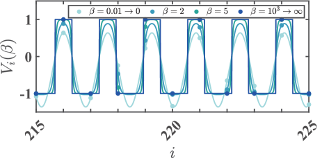
Figure 1: (Color online). Schematic of the quasiperiodically modulated on-site potential (eq. (2)) for several values of $\beta=0.01$, $0.2$, $5$, $1000$ (light to deep blue curves).

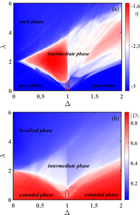
Figure 2: (Color online). Phase diagram that varies with ($\Delta,\lambda$) in terms of $\eta$ (a) and $\langle D\rangle$ (b). The pure phase (intermediate phase) is corresponding to the blue (red) region in (a). The pure phase is further distinguished into extended (deep red region) and localized phase (deep blue region) in (b). The critical phase is persists along $\Delta=1$ with $\lambda\lesssim 0.57$, marked in red elliptic. Here, we set the parameter $\beta=0.01$ and $L=610$.

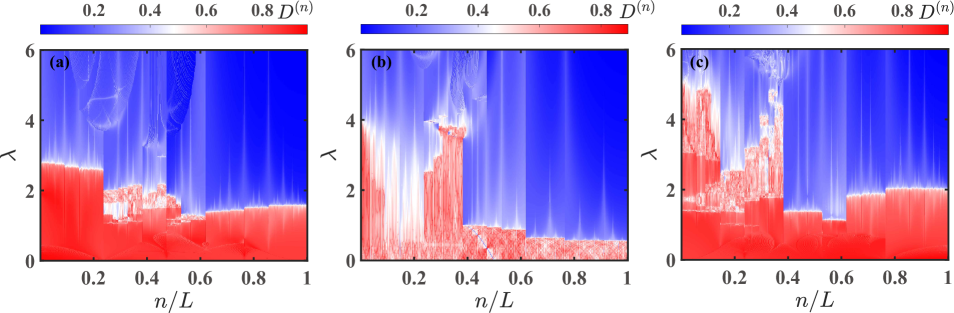
Figure 3: (Color online). (a)-(c) The fractal dimension $D^{(n)}$ versus $\lambda$, where $n$ denotes $n\rm{\mbox{-}th}$ eigenstate of BdG Hamiltonian. The parameter $\Delta$ is $0.5$ (a), $1$ (b) and $1.5$ (c), respectively. Other parameters are $\beta=0.01$ and $L=610$.

Without loss of generality, we set the phase term of the potential to be zero ($\theta=0$). The golden mean ratio $\alpha$ can be derived from the limit of the ratio of consecutive Fibonacci numbers $F_{i}$ Kohmoto (1983): $\alpha=\lim_{n\rightarrow\infty}\frac{F_{n-1}}{F_{n}}=\frac{\sqrt{5}-1}{2}$ with $F_{0}=F_{1}=1$. The parameter $\beta$ serves as a control mechanism allowing interpolation between two known limiting cases of $\beta\rightarrow 0$ and $\beta\rightarrow\infty$. For the former, the potential $V_{i}(\beta)$ simplifies to ${\rm{cos}}(2\pi\alpha i+\theta)-{\rm{cos}}(\pi\alpha)$. Then the model becomes a $1$D p-wave superconductor in the incommensurate lattices Cai et al. (2013) up to a constant on-site chemical potential shift. For the latter, $V_{i}(\beta)$ corresponds to a step potential switching between $\pm 1$ values following the Fibonacci substitution rule. Fig. 1 illustrates the on-site potential $V_{i}(\beta)$ to have a more intuitive understanding.

Considering the Hamiltonian. (1) owns particle-hole symmetry, we can employ the Bogoliubov-de Gennes (BdG) transformation van Hemmen (1980) to diagonalize it, as follows:

$$\hat{\gamma}_{\mu}^{\dagger}=\sum_{i=1}^{L}({v_{i\mu}\hat{c}_{i}+u_{i\mu}\hat{c}_{i}^{\dagger}}),$$ (3)

where $L$ is the number of lattice sites and $\mu=1,...,L$. In this paper, we set $L=F_{n-1}/F_{n}$ to ensure a periodic boundary condition. Then the eq. (1) in terms of the $\hat{\gamma}_{\mu}$ and $\hat{\gamma}_{\mu}^{\dagger}$ operators reads:

$$\hat{H}=\sum_{\mu=1}^{L}2\epsilon_{\mu}(\hat{\gamma}_{\mu}^{\dagger}\hat{\gamma}_{\mu}-\frac{1}{2}).$$ (4)

Assuming the energy spectrum $\epsilon_{\mu}$ is positive. The eigenstates in terms of spinless fermion language is defined as $|\psi\rangle=(u_{\mu 1},...,u_{\mu L},v_{\mu 1},...v_{\mu L})^{T}$ and the positive eigenvalues $\epsilon_{\mu}$ are obtained by solving Bogoliubov-de Gennes equation:

$$\mathcal{\hat{H}}\left(\begin{array}[]{cc}u_{\mu}\\ v_{\mu}\end{array}\right)=\left(\begin{array}[]{cc}A&B\\ -B^{*}&-A^{*}\end{array}\right)\left(\begin{array}[]{cc}u_{\mu}\\ v_{\mu}\end{array}\right)=\epsilon_{\mu}\left(\begin{array}[]{cc}u_{\mu}\\ v_{\mu}\end{array}\right).$$ (13)

All couplings are real in our model, the associated $2L\times 2L$ matrices $\mathcal{\hat{H}}$ is real and symmetric. Hence the matrix $A$ is real and symmetric $(A=A^{*}=A^{T})$, while $B$ is real and anti-symmetric $(B=B^{*}=-B^{T})$. specifically, $2A_{ij}=V_{ij}\delta_{ij}-J(\delta_{j,i+1}+\delta_{j,i-1})$, $2B_{i,j}=-\Delta(\delta_{j,i+1}-\delta_{j,i-1})$. The eigenvector components are defines as $u_{\mu}^{T}=(u_{\mu 1},...,u_{\mu L})^{T}$ and $v_{\mu}^{T}=(v_{\mu 1},...,v_{\mu L})^{T}$. The eigenvalues satisfy $\hat{\gamma}_{\mu}(\epsilon_{\mu})=\hat{\gamma}_{\mu}^{\dagger}(-\epsilon_{\mu})$ where only the zero-energy states $(\epsilon_{\mu}=0)$ are self-conjugate due to the particle-hole symmetry. Our calculations will focus solely on the quasiparticle spectra of the BdG Hamiltonian for simplify.

In this following, we discuss several physical quantities to characterize the nature of wave function. Firstly, we introduce the inverse participation ratio $({\rm{IPR}})$ defined in eq. (15) and the normalized participation ratio $({\rm{NPR}})$ defined in eq. (16), which are utilized to differentiate among the extended, critical and localized states Roy et al. (2023).

$${\rm{IPR}}^{(n)} =\sum_{m=1}^{L}[|u_{m}^{(n)}|^{4}+|v_{m}^{(n)}|^{4}],$$ (15)

$${\rm{NPR}}^{(n)} =[2L\times{\rm{IPR}}^{(n)}]^{-1}.$$ (16)

Where eq. (15) satisfies ${\rm{IPR}}^{(n)}\sim 1/(2L)^{\gamma_{n}}$ Qi et al. (2023). The index $n$ denotes the $n\rm{\mbox{-}th}$ eigenstate of BdG Hamiltonian and $m$ is the $m\rm{\mbox{-}th}$ element of that eigenstate. For the $n\rm{\mbox{-}th}$ eigenstate, when ${\rm{IPR}}$ approaches $0$, it indicates a extended state and the corresponding $\gamma_{n}=1$. Conversely, ${\rm{NPR}}$ approaches $0$ and $\gamma_{n}=0$ for a localized state. If the state is critical, $\gamma_{n}\in(0,1)$.

For a large-size system, the fractal dimension $D^{(n)}$ is defined as follows  Yao et al. (2019); Li and Das Sarma (2020); Qi et al. (2023):

$$D^{(n)}=-\lim_{L\rightarrow\infty}\frac{\log({\rm{IPR}}^{(n)})}{\log 2L}.$$ (17)

By analyzing the inverse participation ratio ${\rm{IPR}}^{(n)}$, we can easily infer that $D^{(n)}$ goes to $0$ ($1$) for the localized (extended) state and $D^{(n)}\in(0,1)$ for the critical state. Then the average fractal dimension $\langle D\rangle$ averaged over the BdG quasiparticle spectrum can capture the overall characteristics of the system and it is defined as:

$$\langle D\rangle=\frac{1}{L}\sum_{n=1}^{L}D^{(n)}.$$ (18)

The system exhibits phases that are either extended, where the average fractal dimension $\langle D\rangle$ approaches $0$, or localized, where $\langle D\rangle$ approaches $1$. However, it cannot distinguish the critical phase from intermediate phase. It is necessary to compute $D^{(n)}$ for each eigenstate, if $D^{(n)}\in(0,1)$ for all the eigenstates, it suggests a critical phase. Furthermore, we define $\overline{D}$ averaged across a subset of eigenstates to capture the different states coexist in an intermediate phase.

Next, we introduce $\eta$ which aids in distinguishing pure phases (extended or localized phase) from intermediate phase, defined as Yao et al. (2019); Li and Das Sarma (2020); Qi et al. (2023),

$$\eta={\rm{log_{10}}}[\langle{\rm{IPR}}\rangle\times\langle{\rm{NPR}}\rangle],$$ (19)

where $\langle{\rm{IPR}}\rangle$ and $\langle{\rm{NPR}}\rangle$ are given by eq. (20). For the extended phase, $\langle{\rm{IPR}}\rangle\rightarrow 0$ [$\langle{\rm{NPR}}\rangle\rightarrow$ finite]. Conversely, for the localized phase, $\langle{\rm{NPR}}\rangle\rightarrow 0$ [$\langle{\rm{IPR}}\rangle\rightarrow$ finite]. So we have $\langle{\rm{IPR}}\rangle\times\langle{\rm{NPR}}\rangle\sim 1/2L$ and $\eta\lesssim-3$ in the pure phases, where $L=610$ in Fig. 2. For the intermediate phase, both of $\langle{\rm{IPR}}\rangle$ and $\langle{\rm{NPR}}\rangle$ keep finite and $-3<\eta\lesssim-1$.

$$\langle\mathrm{IPR}\rangle=\frac{1}{L}\sum_{n=1}^{L}\mathrm{IPR}_{n}, \langle\mathrm{NPR}\rangle=\frac{1}{L}\sum_{n=1}^{L}\mathrm{NPR}_{n}.$$ (20)

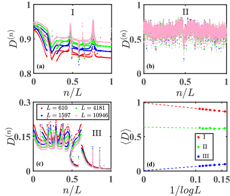
Figure 4: (Color online). (a)-(c) The fractal dimension $D^{(n)}$ for different $L$ at fixed $\Delta=0.5$ and $\lambda=0.2$ (a), $\Delta=1$ and $\lambda=0.2$ (b), $\Delta=0.5$ and $\lambda=5.8$ (c), where $n$ denotes $n\rm{\mbox{-}th}$ eigenstate. (d) Finite-size extrapolation of $\langle D\rangle$ as a function $1/\rm{log}(L)$.

III phase diagram for Small $\beta$

As mentioned above, the potential $V_{i}(\beta)$ simplifies to $\rm{cos(2\pi\alpha i+\theta)-cos(\pi\alpha)}$ in small $\beta$ limit. It differs from the previous study which exclusively considered a cosine potential without the constant on-site chemical potential shift Cai et al. (2013). In order to substantiate this distinction, we show the phase diagram where variable $\eta$ and fractal dimension $\langle D\rangle$ versus ($\lambda$, $\Delta$) in Fig. 2. This diagram features two distinct regions: the pure phases (depicted in blue) and the intermediate phases (depicted in red) separated by $\eta$ in Fig. 2(a). And the pure phases are further distinguished into extended phases (deep red region) and localized phases (deep blue region) by $\langle D\rangle$ in Fig. 2(b).

In order to have a complete insight into the phase diagram, we calculate the fractal dimension $D^{(n)}$ where $n$ denotes $n\rm{\mbox{-}th}$ eigenstate of BdG Hamiltonian versus the potential strength $\lambda$ for different $\Delta=0.5$, $1$ and $1.5$, as illustrated in Fig. 3. It is interesting that the critical phase is confined to a narrow line where $\Delta=1$ and $\lambda\lesssim 0.57$. Therefore, the complete phase diagram includes three pure phases (extended, localized and critical phase) and many types of intermediate phases. A more detailed discussion of these phases will be provided in subsequent sections.

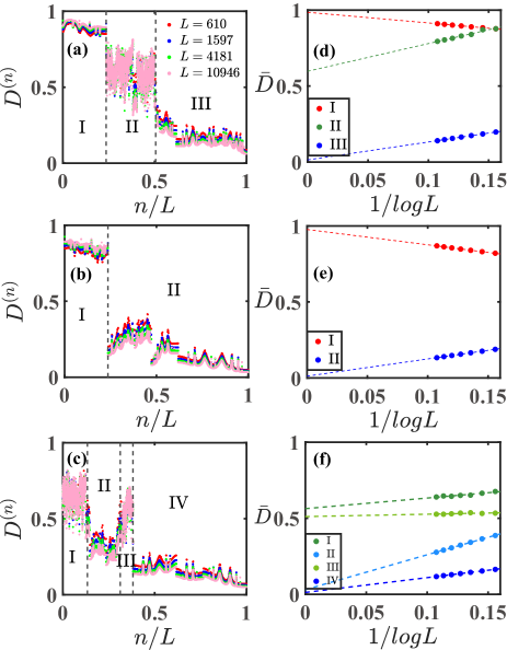
Figure 5: (Color online). (a)-(c) The fractal dimension $D^{(n)}$ for different $L$ at fixed $\Delta=0.5$ and $\lambda=1.8$ (a), $\Delta=0.5$ and $\lambda=2.3$ (b), $\Delta=1.5$ and $\lambda=3.5$ (c), where $n$ denotes $n\rm{\mbox{-}th}$ eigenstate. (d)-(f) Finite-size extrapolation of $\langle D\rangle$ as a function $1/\rm{log}(L)$ averaged over the different state zones in (a)-(c).

III.1 Pure phases

Fig. 33 shows the system is in the extended (critical) phase where all the states are extended (critical) when $\Delta\neq 1$ ($\Delta=1$), with weak potential strength $\lambda$. To provide more precise numerical evidences, we further calculate the $D^{(n)}$ for various lattice sizes $L$ at selected values of $\lambda$, the results are displayed in Fig. 4(a)-(b). And the finite-size extrapolation of $\langle D\rangle$ averaged over the quasiparticle spectrum is shown in Fig. 4(d). Take $\Delta=0.5$ and $\lambda=0.2$ for example, Fig. 4(a) shows the $D^{(n)}$ for all the states increase with $L$ and the $\langle D\rangle$ approach $1$ in the thermodynamic limit, indicating the system is in the extended phase. Additionally, when $\Delta=1$, the $D^{(n)}$ fluctuates from $0$ and $1$, independent on $L$, indicating all the states are critical, as shown in Fig. 4(b). When the potential strength $\lambda$ is strong enough, such as $\lambda=5.8$ for $\Delta=0.5$, the system goes to a localized phase where $D^{(n)}$ tends to $0$ for all the states, as shown in Fig. 4(c). Therefore, the system exhibits three distinct pure phases, including extended, critical and localized phase.

III.2 Intermediate phases

One can observe that the system undergoes various intermediate phases before transitioning into the localized phase as shown in Fig. 3. When $\Delta=0.5$ and $\lambda=1.8$ as shown in Fig. 5(a) (d), $D^{(n)}$ corresponding to the low energy states in zone $\rm{I}$ increase with $L$, and the finite-size extrapolation of $\overline{D}$ averaged over the zone $\rm{I}$ goes to $1$, indicating all the states in zone $\rm{I}$ are extended. While $D^{(n)}$ corresponding to the high energy states in zone $\rm{III}$ decrease with $L$, and the finite-size extrapolation of $\overline{D}$ averaged over the zone $\rm{III}$ goes to $0$, indicating all the states in zone $\rm{III}$ are localized. In contrast, $D^{(n)}$ for the states in zone $\rm{II}$ fluctuates around $0.6$, almost independent of $L$, and the finite-size extrapolation of $\overline{D}$ averaged over the zone $\rm{II}$ approaches a finite value between $0$ and $1$, indicating all the states in zone $\rm{II}$ are critical. Hence the system exhibits an intermediate phase with coexisting localized, extended, and critical states. These states are separated by the two types of anomalous mobility edge separating extended or localized from critical states. When $\lambda$ is slightly increased (i.e., $\lambda=2.3$) shown in Fig. 5(b)(e), we identify another intermediate phase with coexisting localized and extended states where $\overline{D}$ goes to $1$ ($\rm{I}$) and $0$ ($\rm{II}$) in the thermodynamic limit, respectively. This intermediate phase exhibits a traditional mobility edge separating the extended and localized zones. When the $\Delta=1.5$ and $\lambda=3.5$ shown in Fig. 5(c)(f), $D^{(n)}$ for states in zones $\rm{II}$ and $\rm{IV}$ decrease with $L$ and its average value $\overline{D}$ goes to $0$, indicating they are localized. Conversely, $D^{(n)}$ fluctuates around $0.56$ and $0.5$ for states in zones $\rm{I}$ and $\rm{III}$ , indicating the states are critical. Therefore, the system has an intermediate phase with coexisting localized and critical states. These states in different zones are separated by an anomalous mobility edge.

The system is known to exhibit a critical phase when $\Delta=0.1$ and $\lambda\lesssim 0.57$ (see Sec. III.1). Additionally, a distinct intermediate phase emerges when $\Delta$ is slightly deviating from $1$. Now take $\lambda=0.2$ for example, Fig. 6(a) shows that the $\langle D\rangle$ varies smoothly versus $\Delta$ when $\Delta\lesssim 0.92$. A notable decrease in $\langle D\rangle$ is first observed when the system goes into the intermediate phase with coexisting extended ($\rm{I}$) and critical states ($\rm{II}$), as shown in Fig. 6(b). Subsequently, a second notable decline occurs when the system enters the critical phase with $\Delta=1$ [see Fig. 4(b)]. The phenomenon is easily understand by the ultimate value of $D^{(n)}$ is less than $1$ in the thermodynamic limit for the critical states. Consequently, the system exhibits four distinct intermediate phases: the first one with coexisting extended and localized states; the second one with coexisting extended and critical states; the third one with coexisting localized and critical states; and the fourth one with coexisting extended, critical, and localized states.

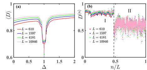
Figure 6: (Color online). (a) The fractal dimension $\langle D\rangle$ averaged over all the BdG quasiparticle spectrum versus $\Delta$. (b) The fractal dimension $D^{(n)}$ for different $L$ at $\Delta=1$, where $n$ denotes $n\rm{\mbox{-}th}$ eigenstate. The parameter $\lambda=0.2$.

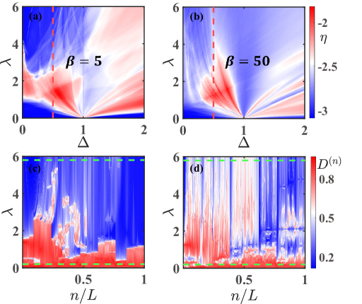
Figure 7: (Color online). (a)-(b) Phase diagram of variable $\eta$ versus ($\Delta,\lambda$). The red dashed line corresponds to $\Delta=0.5$. (c)-(d) The fractal dimension $D^{(n)}$ versus $\lambda$, where $n$ denotes $n\rm{\mbox{-}th}$ eigenstate of BdG Hamiltonian when $\Delta=0.5$. The green dashed lines corresponds to $\lambda=0.2$ and $5.8$, respectively. Here, the parameter $\beta=5$ (a)(c), $50$ (b)(d) and $L=610$ .

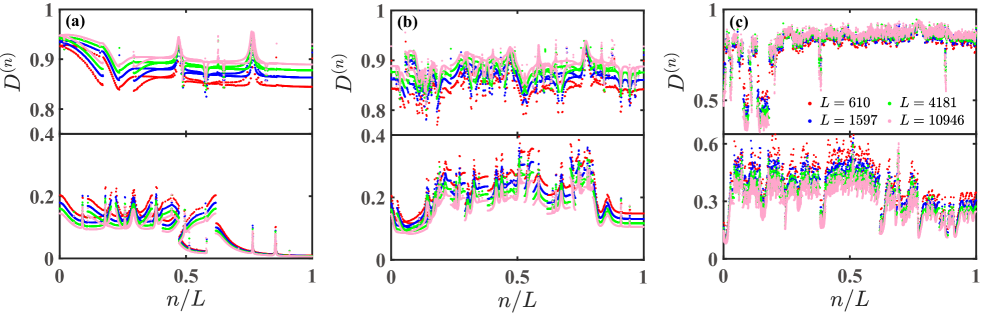
Figure 8: (Color online). The fractal dimension $D^{(n)}$ for different $L$ at fixed $\beta=0.01$ (a), $\beta=5$ (b), $\Delta=50$ (c), where $n$ denotes $n\rm{\mbox{-}th}$ eigenstate. Other parameters $\Delta=0.5$ and $\lambda=0.2$ ($5.8$) for the upper (lower) panel of each figure. .

IV phase diagram with increasing $\beta$

In order to investigate the effect of increasing $\beta$, we begin by analyzing the phase diagram where variable $\eta$ versus ($\lambda$, $\Delta$) at fixed $\beta=5$ and $\beta=50$, as shown in Fig. 7(a) and (b). In contrast to the phase diagram shown in Fig. 2(a), we found that the zones for pure phases such as extended phase and localized phase are significantly diminished with increasing $\beta$. We plot the fractal dimension $D^{(n)}$ versus $\lambda$ at fixed $\Delta=0.5$ in Fig. 7(c)-(d). Fig. 7(c) shows that an extensive number of extended states are replaced by the critical states or localized states when the strength of potential is weak, which differs markedly from the scenario presented in Fig. 3(a). As the strength of potential $\lambda$ increases, the system exhibits various intermediates phases, such as one comprising both localized and critical states, and another with coexisting extended, critical and localized states. What is more, the system goes to the localized phase when the strength of potential is further increased. Hence, the phase diagram does not have essential changes when $\beta=5$. However, the pure phases (extended or localized phase) almost disappear when further increasing $\beta$, and more critical states emerge despite of how much the value of $\lambda$, as shown in Fig. 7(d).

To illustrate the impact of $\beta$ on the system, we examine the fractal dimension $D^{(n)}$ for different $L$ at a fixed weak $\lambda=0.2$ and a strong $\lambda=5.8$, with $\beta$ ranging from small to large, as shown in the upper and lower panels of Fig. 8, respectively. The $D^{(n)}$ goes to $1$ ($0$) with the increase of $L$ when $\beta=0.01$, representing a completely extended (localized) phase, as shown in Fig. 8(a). At $\beta=5$, $D^{(n)}$ exhibits minor fluctuations for a limited number of states, suggesting a slightly deviation from pure phase, yet without significantly altering its essence, as shown in Fig. 8(b). However, this fluctuation becomes pronounced at higher $\beta$ values. Fig. 8(c) reveals that $D^{(n)}$ fluctuates between $0$ and $1$ for most states, indicating the critical states. Hence the system has an intermediate phase with coexisting mostly critical states and rarely localized states. One can infer that the localized states will disappear with further increments in $\beta$, and the system is finally in the critical phase.

V Conclusion and outlook

In summary, our research delineates the various quantum phases emerged in the IAAF model with p-wave SC pairing terms. This model exhibits modifiable phase diagrams through the tunable parameter $\beta$. For small values of $\beta$, this model can be reduced to the generalized AA model up to a constant on-site chemical potential shift. The system is always in the pure phases when the strength of potential is weak (extended or critical phase) or strong (localized phase) enough. What is more, it is interesting that the system has many types of intermediate phases when the strength of potential is moderate. For instance, one can observe an intermediate phase where extended and localized states coexist, as well as phases where extended and critical states, or localized and critical states, are present concurrently. Also, the coexistence of extended, critical and localized states. These coexisting states are separated by different type of mobility edges. As $\beta$ increase, the pure phases (extended or localized phase) will gradually diminish, and the system becomes critical in the Fibonacci limit.

This work unveils a quantum model that exhibits many types of intermediate phases, thereby enriching the understanding of mobility edges. A natural question is that whether these intermediate phases are robust when interactions are introduced. Additionally, investigating the dynamic properties that arise from the various phases may be another intriguing question. Besides, the one-dimensional (1D) p-wave superconducting paired fermion model can be mapped onto the transverse XY model via the Jordan-Wigner transformation Fisher (1995); Young and Rieger (1996). Our research casts a new light on the study of analogous phenomena related to localization in low-dimensional quasi-periodic spin systems.

VI Acknowledgments

We thank Zi Cai for useful discussions. This work is supported by the National Key Research and Development Program of China (Grant No. 2020YFA0309000), NSFC of China (Grant No.12174251), the Natural Science Foundation of Shanghai (Grant No.22ZR142830), and the Shanghai Municipal Science and Technology Major Project (Grant No. 2019SHZDZX01).

References

- Anderson (1958) P. W. Anderson, Phys. Rev. 109, 1492 (1958).
- Abrahams et al. (1979) E. Abrahams, P. W. Anderson, D. C. Licciardello, and T. V. Ramakrishnan, Phys. Rev. Lett. 42, 673 (1979).
- Lee and Ramakrishnan (1985) P. A. Lee and T. V. Ramakrishnan, Rev. Mod. Phys. 57, 287 (1985).
- Evers and Mirlin (2008) F. Evers and A. D. Mirlin, Rev. Mod. Phys. 80, 1355 (2008).
- Lahini et al. (2009) Y. Lahini, R. Pugatch, F. Pozzi, M. Sorel, R. Morandotti, N. Davidson, and Y. Silberberg, Phys. Rev. Lett. 103, 013901 (2009).
- Kraus et al. (2012) Y. E. Kraus, Y. Lahini, Z. Ringel, M. Verbin, and O. Zilberberg, Phys. Rev. Lett. 109, 106402 (2012).
- Wang et al. (2020a) P. Wang, Y. Zheng, X. Chen, C. Huang, C. Huang, Y. V. Kartashov, L. Torner, V. V. Konotop, and F. Ye, Nature 577, 42–46 (2020a).
- Roati et al. (2008) G. Roati, C. D’Errico, L. Fallani, M. Fattori, C. Fort, M. Zaccanti, G. Modugno, M. Modugno, and M. Inguscio, Nature 453, 895–898 (2008).
- Modugno (2010) G. Modugno, Reports on Progress in Physics 73, 102401 (2010).
- Gredeskul and Kivshar (1989) S. A. Gredeskul and Y. S. Kivshar, Phys. Rev. Lett. 62, 977 (1989).
- Christodoulides et al. (2003) D. N. Christodoulides, F. Lederer, and Y. Silberberg, Nature 424, 817 (2003).
- Pertsch et al. (2004) T. Pertsch, U. Peschel, J. Kobelke, K. Schuster, H. Bartelt, S. Nolte, A. Tünnermann, and F. Lederer, Phys. Rev. Lett. 93, 053901 (2004).
- Aubry and André (1980) S. Aubry and G. André, Ann. Isr. Phys. 3 (1980).
- Kohmoto et al. (1983) M. Kohmoto, L. P. Kadanoff, and C. Tang, Phys. Rev. Lett. 50, 1870 (1983).
- Ostlund et al. (1983) S. Ostlund, R. Pandit, D. Rand, H. J. Schellnhuber, and E. D. Siggia, Phys. Rev. Lett. 50, 1873 (1983).
- Merlin et al. (1985) R. Merlin, K. Bajema, R. Clarke, F. Y. Juang, and P. K. Bhattacharya, Phys. Rev. Lett. 55, 1768 (1985).
- Ashraff and Stinchcombe (1989) J. A. Ashraff and R. B. Stinchcombe, Phys. Rev. B 40, 2278 (1989).
- Roche et al. (1997) S. Roche, G. Trambly de Laissardière, and D. Mayou, Journal of Mathematical Physics 38, 1794 (1997).
- Maciá (1999) E. Maciá, Phys. Rev. B 60, 10032 (1999).
- Domińguez-Adame (2001) F. Domińguez-Adame, Physica B: Condensed Matter 307, 247 (2001).
- Macé et al. (2017) N. Macé, A. Jagannathan, P. Kalugin, R. Mosseri, and F. Piéchon, Phys. Rev. B 96, 045138 (2017).
- Jagannathan (2021) A. Jagannathan, Rev. Mod. Phys. 93, 045001 (2021).
- Raymond Aschheim and Irwin (2023) D. C. Raymond Aschheim, David Chester and K. Irwin, Quaestiones Mathematicae 46, 2475 (2023).
- Dal Negro et al. (2003) L. Dal Negro, C. J. Oton, Z. Gaburro, L. Pavesi, P. Johnson, A. Lagendijk, R. Righini, M. Colocci, and D. S. Wiersma, Phys. Rev. Lett. 90, 055501 (2003).
- Tanese et al. (2014) D. Tanese, E. Gurevich, F. Baboux, T. Jacqmin, A. Lemaître, E. Galopin, I. Sagnes, A. Amo, J. Bloch, and E. Akkermans, Phys. Rev. Lett. 112, 146404 (2014).
- Baboux et al. (2017) F. Baboux, E. Levy, A. Lemaître, C. Gómez, E. Galopin, L. Le Gratiet, I. Sagnes, A. Amo, J. Bloch, and E. Akkermans, Phys. Rev. B 95, 161114 (2017).
- Reisner et al. (2023) M. Reisner, Y. Tahmi, F. Piéchon, U. Kuhl, and F. Mortessagne, Phys. Rev. B 108, 064210 (2023).
- Kraus and Zilberberg (2012) Y. E. Kraus and O. Zilberberg, Phys. Rev. Lett. 109, 116404 (2012).
- Verbin et al. (2013) M. Verbin, O. Zilberberg, Y. E. Kraus, Y. Lahini, and Y. Silberberg, Phys. Rev. Lett. 110, 076403 (2013).
- Verbin et al. (2015) M. Verbin, O. Zilberberg, Y. Lahini, Y. E. Kraus, and Y. Silberberg, Phys. Rev. B 91, 064201 (2015).
- Goblot et al. (2020) V. Goblot, A. Štrkalj, N. Pernet, J. L. Lado, C. Dorow, A. Lemaître, L. Le Gratiet, A. Harouri, I. Sagnes, S. Ravets, A. Amo, J. Bloch, and O. Zilberberg, Nature Physics 16, 832 (2020).
- Zhai et al. (2021) L.-J. Zhai, G.-Y. Huang, and S. Yin, Phys. Rev. B 104, 014202 (2021).
- Štrkalj et al. (2021) A. Štrkalj, E. V. H. Doggen, I. V. Gornyi, and O. Zilberberg, Phys. Rev. Res. 3, 033257 (2021).
- Dai et al. (2023) Q. Dai, Z. Lu, and Z. Xu, Phys. Rev. B 108, 144207 (2023).
- Whitney (2014) R. S. Whitney, Phys. Rev. Lett. 112, 130601 (2014).
- Yamamoto et al. (2017) K. Yamamoto, A. Aharony, O. Entin-Wohlman, and N. Hatano, Phys. Rev. B 96, 155201 (2017).
- Chiaracane et al. (2020) C. Chiaracane, M. T. Mitchison, A. Purkayastha, G. Haack, and J. Goold, Phys. Rev. Res. 2, 013093 (2020).
- Das Sarma et al. (1988) S. Das Sarma, S. He, and X. C. Xie, Phys. Rev. Lett. 61, 2144 (1988).
- Biddle and Das Sarma (2010) J. Biddle and S. Das Sarma, Phys. Rev. Lett. 104, 070601 (2010).
- Biddle et al. (2009) J. Biddle, B. Wang, D. J. Priour, and S. Das Sarma, Phys. Rev. A 80, 021603 (2009).
- Wang et al. (2020b) Y. Wang, X. Xia, L. Zhang, H. Yao, S. Chen, J. You, Q. Zhou, and X.-J. Liu, Phys. Rev. Lett. 125, 196604 (2020b).
- Roy et al. (2021) S. Roy, T. Mishra, B. Tanatar, and S. Basu, Phys. Rev. Lett. 126, 106803 (2021).
- Zhou et al. (2023) X.-C. Zhou, Y. Wang, T.-F. J. Poon, Q. Zhou, and X.-J. Liu, Phys. Rev. Lett. 131, 176401 (2023).
- Das Sarma et al. (1990) S. Das Sarma, S. He, and X. C. Xie, Phys. Rev. B 41, 5544 (1990).
- Ganeshan et al. (2015) S. Ganeshan, J. H. Pixley, and S. Das Sarma, Phys. Rev. Lett. 114, 146601 (2015).
- Li et al. (2017) X. Li, X. Li, and S. Das Sarma, Phys. Rev. B 96, 085119 (2017).
- Lüschen et al. (2018) H. P. Lüschen, S. Scherg, T. Kohlert, M. Schreiber, P. Bordia, X. Li, S. Das Sarma, and I. Bloch, Phys. Rev. Lett. 120, 160404 (2018).
- Yao et al. (2019) H. Yao, A. Khoudli, L. Bresque, and L. Sanchez-Palencia, Phys. Rev. Lett. 123, 070405 (2019).
- Li and Das Sarma (2020) X. Li and S. Das Sarma, Phys. Rev. B 101, 064203 (2020).
- Qi et al. (2023) R. Qi, J. Cao, and X.-P. Jiang, Phys. Rev. B 107, 224201 (2023).
- Hatsugai and Kohmoto (1990) Y. Hatsugai and M. Kohmoto, Phys. Rev. B 42, 8282 (1990).
- Takada et al. (2004) Y. Takada, K. Ino, and M. Yamanaka, Phys. Rev. E 70, 066203 (2004).
- Wang et al. (2016) J. Wang, X.-J. Liu, G. Xianlong, and H. Hu, Phys. Rev. B 93, 104504 (2016).
- Liu et al. (2015) F. Liu, S. Ghosh, and Y. D. Chong, Phys. Rev. B 91, 014108 (2015).
- Wang et al. (2022) Y. Wang, L. Zhang, W. Sun, T.-F. J. Poon, and X.-J. Liu, Phys. Rev. B 106, L140203 (2022).
- Roy et al. (2023) S. Roy, S. N. Nabi, and S. Basu, Phys. Rev. B 107, 014202 (2023).
- Lin et al. (2023) X. Lin, X. Chen, G.-C. Guo, and M. Gong, Phys. Rev. B 108, 174206 (2023).
- Li and Li (2023) S.-Z. Li and Z. Li, arXiv:2304.11811 (2023).
- Kohmoto (1983) M. Kohmoto, Phys. Rev. Lett. 51, 1198 (1983).
- Cai et al. (2013) X. Cai, L.-J. Lang, S. Chen, and Y. Wang, Phys. Rev. Lett. 110, 176403 (2013).
- van Hemmen (1980) J. L. van Hemmen, Zeitschrift fr Physik B Condensed Matter 38, 271 (1980).
- Fisher (1995) D. S. Fisher, Phys. Rev. B 51, 6411 (1995).
- Young and Rieger (1996) A. P. Young and H. Rieger, Phys. Rev. B 53, 8486 (1996).