31st January 2024

Compton Scattering on ⁴He with Nuclear One- and Two-Body Densities

Harald W. Grießhammer^abc, Junjie Liao^a, Judith A. McGovern^d,

Andreas Nogga^e and Daniel R. Phillips^fg

^a Institute for Nuclear Studies, Department of Physics,
The George Washington University, Washington DC 20052, USA

^b Department of Physics, Duke University, Box 90305, Durham NC 27708, USA

^c High Intensity Gamma-Ray Source, Triangle Universities Nuclear Laboratories,
Box 90308, Durham NC 27708, USA

^d Department of Physics and Astronomy, The University of Manchester,
Manchester M13 9PL, UK

^e IAS-4, IKP-3 and JCHP, Forschungszentrum Jülich, D-52428 Jülich, Germany

^f Department of Physics and Astronomy and Institute of Nuclear and Particle Physics,
Ohio University, Athens OH 45701, USA

^gDepartment of Physics, Chalmers University of Technology, SE-41296 Göteborg, Sweden

We present the first ab initio calculation of elastic Compton scattering from ⁴He. It is carried out to $\mathcal{O}(e^{2}\delta^{3})$ [N³LO ] in the $\delta$ expansion of $\chi$EFT. At this order and for this target, the only free parameters are the scalar-isoscalar electric and magnetic dipole polarisabilities of the nucleon. Adopting current values for these yields a parameter-free prediction. This compares favourably with the world data from HI$\gamma$S, Illinois and Lund for photon energies $50\;\mathrm{MeV}\lesssim\omega\lesssim 120\;\mathrm{MeV}$ within our theoretical uncertainties of $\pm 10\%$. We predict a cross section up to 7 times that for deuterium. As in ³He, this emphasises and tests the key role of meson-exchange currents between $\mathrm{n}\mathrm{p}$ pairs in Compton scattering on light nuclei. We assess the sensitivity of the cross section and beam asymmetry to the nucleon polarisabilities, providing clear guidance to future experiments seeking to further constrain them. The calculation becomes tractable by use of the Transition Density Method. The one- and two-body densities generated from $5$ chiral potentials and the AV18$+$UIX potential are available using the python package provided at https://pypi.org/project/nucdens/.

Suggested Keywords: Chiral Effective Field Theory, proton, neutron and nucleon polarisabilities, ⁴He Compton scattering, $\Delta(1232)$ resonance, pion-exchange currents, Transition Density Method

1 Introduction

The elastic scattering of photons with energies between approximately 50 MeV and the first resonance region from bound few-nucleon systems, $\gamma A\to\gamma A$, examines two fundamental and connected aspects of the electromagnetic structure of hadrons and nuclei. First, this coherent Compton scattering reaction yields determinations of the neutron electric and magnetic scalar dipole polarisabilities from data. Second, it showcases the marked impact of two-body currents mediated by charged pion exchange. Since both these aspects of QCD’s spontaneously and dynamically broken chiral symmetry are leading contributions to the nuclear Compton response at photon energies $\omega\sim m_{\pi}$, this process can provide profound insight—but only if the answers across different nuclei are consistent.

Indeed, Compton scattering reactions on the proton and the lightest nuclei have been a vigorous area of experimental and theoretical activity over the last twenty-five years, with the goal being to deliver experimental systematic uncertainties and theoretical accuracy that will elucidate these aspects of QCD. The rationale for and goals of this international effort are described in a recent White Paper [1] and review [2]. The nucleon’s electric and magnetic dipole polarisabilities $\alpha_{E1}$ and $\beta_{M1}$ characterise the extent to which the nucleon acquires an induced electric and magnetic dipole moment in external electromagnetic fields; they therefore determine the induced radiation dipoles [2]. Compton scattering from the lightest nuclei, where the theory of nuclear electromagnetic responses is most under control, is our best opportunity to determine the value of these fundamental neutron structure parameters.

Chiral Effective Field Theory ($\chi$EFT) is used to interpret such data. $\chi$EFT describes both the structure of nuclear targets and the electromagnetic operators that encode the coupling of photons to the degrees of freedom inside the nucleus. It is a model-independent approach that organises the low-energy dynamics of strongly interacting systems in powers of a small expansion parameter. Theory uncertainties associated with truncation of the $\chi$EFT expansion can therefore be estimated.

Thus far, the best neutron polarisability values are inferred from a 2015/18 $\chi$EFT fit to deuteron Compton data [3, 4, 5]. The scalar-isoscalar polarisabilities obtained are

$$\alpha_{E1}^{(\mathrm{s})}=11.1\pm 0.6_{\mathrm{stat}}\pm 0.2_{\mathrm{BSR}}\pm 0.8_{\mathrm{th}}\;\;,\;\;\beta_{M1}^{(\mathrm{s})}=3.4\mp 0.6_{\mathrm{stat}}\pm 0.2_{\mathrm{BSR}}\pm 0.8_{\mathrm{th}}$$ (1.1)

in the canonical units for scalar polarisabilities of $10^{-4}\leavevmode\nobreak\ \mathrm{fm}^{3}$ employed throughout. Note that these works also estimated the theory uncertainty from omitted higher-order terms in $\chi$EFT. And indeed, those uncertainties—together with the point-to-point errors of the deuteron Compton data—dominate the final uncertainty on the neutron numbers because they are markedly larger than the corresponding uncertainties in the case of the proton:

$$\alpha_{E1}^{(\mathrm{p})}=10.65\pm 0.35_{\text{stat}}\pm 0.2_{\text{Baldin}}\pm 0.3_{\text{th}}\;\;,\;\;\beta_{M1}^{(\mathrm{p})}=3.15\mp 0.35_{\text{stat}}\pm 0.2_{\text{Baldin}}\mp 0.3_{\text{th}}\;\;.$$ (1.2)

This leads to a lack of clarity on the sign of the proton-neutron polarisability difference, and only limited knowledge of its size:

$$\alpha_{E1}^{(\mathrm{p})}-\alpha_{E1}^{(\mathrm{n})}=[-0.9\pm 1.6_{\text{tot}}]\;\;.$$ (1.3)

Meanwhile, lattice-QCD determinations remain challenging; see e.g. [5, 9, 10, 11, 12, 13]. More work is clearly needed for a better understanding of the degree to which proton and neutron polarisabilities differ: data and theory must be improved such that the overall uncertainty in the extraction of $\alpha_{E1}^{(\mathrm{p})}-\alpha_{E1}^{(\mathrm{n})}$ is shrunk to about one third of its present size. This is especially important as such experimental information will check a finding of the Cottingham Sum Rule for the electromagnetic self-energy correction to the proton-neutron mass difference: $\alpha_{E1}^{(\mathrm{p})}-\alpha_{E1}^{(\mathrm{n})}=[-1.7\pm 0.4]$ [14]; cf. [15, 16, 17, 18]. $\chi$EFT predicts strong $m_{\pi}$-dependence of this difference, which may be related to anthropic arguments [5].

The same scalar-isoscalar polarisability combinations $\alpha_{E1}^{(\mathrm{s})}:=\frac{1}{2}[\alpha_{E1}^{(\mathrm{p})}+\alpha_{E1}^{(\mathrm{n})}]$ etc. are probed in ⁴He as in the isoscalar deuteron. But, because ⁴He is a scalar, the analysis is now free of contamination from spin polarisabilities which play a nontrivial rôle in proton extractions [19]. A ⁴He target also has several experimental advantages that mean measurements using it can deliver a more accurate result. It is inert and thus safe to handle, liquefies at relatively high temperatures, and its high dissociation energy makes for a clear and simple differentiation between elastic and inelastic events even with detectors of low energy resolution. Moreover, cross sections are larger by a factor of 5-to-7 than those for $\gamma$-deuteron scattering.

In this work, we extend the proton, deuteron and ³He Compton analysis in $\chi$EFT to ⁴He. This is also the first ab initio computation (in the sense of ref. [20]) of this reaction, cf. a phenomenological approach employed in ref. [21]. It shows that the growth of the Compton cross section with nuclear mass number is driven by the charged-meson-exchange currents discussed in the opening paragraph. We adopt the polarisability values of eq. (1.1) as input so that $\chi$EFT has no free parameters at the order we consider. The resulting parameter-free calculation predicts the correct size and shape of the Compton cross section.

In the four-nucleon system, the Transition Density Method [23] has already been applied for dark matter-nucleus scattering [24]; we now employ it in Compton kinematics. Since this method markedly simplifies and accelerates the calculation, two-body current implementations become tractable for $A>3$. It does this by separating the Compton process into an interaction kernel of nucleons which do react with the photons, and a background density of nucleons which do not, with the quantum numbers of the latter being traced over before the density is folded with Compton-scattering operators.

The resulting description at $\mathcal{O}(e^{2}\delta^{3})$ in $\chi$EFT may not suffice to reliably extract polarisabilities from ⁴He data, but it does permit reliable investigations of the sensitivity of observables to the scalar-isoscalar dipole polarisabilities. This is useful for current planning of experiments—as we previously argued for a calculation at the same order in ³He [25]. Therefore, a subsidiary goal in this article is an exploratory study of the size of the ⁴He elastic Compton differential cross section and its sensitivity to the nucleon polarisabilities.

To that end, we concentrate on the energy region $50\;\mathrm{MeV}\lesssim\omega\lesssim 120\;\mathrm{MeV}$ where polarisabilities are most likely to be extracted—this was also the domain studied in the first calculations of Compton scattering on deuterium and ³He [26, 27, 28, 29]. In this régime, coherent scattering of photons on ⁴He as a whole is suppressed. At higher energies, that mechanism only serves to reduce the dependence on the $2\mathrm{N}$ and $3\mathrm{N}$ interactions that describe the bound system; see sect. 2.3. The coherent propagation of the $A$-nucleon system between the two photon interactions of the Compton reaction is a key ingredient in the generation of the correct Thomson limit for the nuclear Compton amplitude at lower energies $\omega\to 0$. Meanwhile, at higher energies, $\omega\to m_{\pi}$, the pion-production threshold poses additional experimental and theoretical issues which we do not address here.

The article is organised as follows. In sect. 2, we describe the theoretical ingredients of our approach, starting with a brief and intuition-focused recapitulation of the Transition Density Method (sect. 2.1). Compton observables (sect. 2.2) and the photon-nucleon Compton kernels we already used in the deuteron and ³He are summarised (sect. 2.3), as well as details of the generation of the transition densities (sect. 2.4). Section 3 is devoted to our results, starting with an overview and comparison to data. In sect. 3.3, we quantify the theory uncertainties of our approach as generically $\pm 10\%$ in the cross section—possibly rising to $\pm 12\%$ in back-scattering at the highest energies. The sensitivity of the cross section to varying the polarisabilities is assessed in sect. 3.4. The beam asymmetry is considered in sect. 3.5, followed by a comparison of the ⁴He results to those on the other light nuclei (sect. 3.6). Summary, conclusions and future work are the topic of sect. 4. A preview of the findings reported here was published in ref. [30].

2 Formalism

2.1 The Transition Density Method

We use the Transition Density Method as introduced in refs. [23, 24]. It factorises the interaction of a probe with a nucleus of $A$ nucleons into an interaction kernel between the probe and the $n$ active nucleons which directly interact with it, and a backdrop of $A-n$ spectator nucleons which do not. The effect of the spectators is subsumed into a $n$-body density, namely a transition probability density amplitude that $n$ active nucleons with a specific set of quantum numbers are found inside the nucleus before the interaction, and are re-arranged into another specific set of quantum numbers after it. Figure 1 illustrates this separation, with the interaction kernel depicted as an arrow. It should be stressed that this separation into “active” and “spectator” nucleons is a purely technical one that relies on no approximations beyond those used in more standard evaluations.

An obvious advantage of this factorisation is that densities of the same nucleus can be recycled with different interaction kernels, while the same interaction kernels can be used in different nuclei. For example, we checked that the numerical implementation of our ⁴He densities with kernels describing elastic electron scattering reproduce the well-known electric form factor. Work is also in progress to use the same ³He and ⁴He densities with kernels describing other coherent processes [31]. In turn, for Compton scattering on ⁴He, we use the same kernels as for the ³He results [25]. This brings all Compton processes under one unified framework. Ref. [23] also demonstrated that results are numerically identical to that of the more traditional approach [27, 32, 28, 29, 25], while an orders-of-magnitude reduction of the computational effort facilitates better-converged numerics. This computational speed-up can mainly be attributed to the fact that the production of the densities relies on well-developed modern numerical few-body techniques, while the kernel convolutions only involve sums over a limited range of quantum numbers, plus two three-dimensional integrations in the two-body case; see below. For ⁴He, production times per energy and angle on 2 nodes with 256 CPUs in total on Jureca are about $1$ minute (or about $4$ CPU hours) for one-body densities and $3$ minutes (or about $13$ CPU hours) for two-body ones. Once the densities are in hand, the summation over one-body quantum numbers is near-instantaneous. For two-body matrix elements, summation over quantum numbers in the $(12)$ subsystem as well as—since they, too, are undetected—angular and radial integrations over its incoming and outgoing relative momenta (cf. eq. (2.3) below) adds less than a CPU hour per energy and angle on a workstation to achieve better-than-$0.7\%$ numerical accuracy; see sect. 3.3.4.

It is a fundamental advantage of $\chi$EFT that it provides a well-defined procedure to predict a hierarchy of $n$-body interaction kernels [33, 34, 35, 36, 37, 38]; see also refs. [39, 40, 41, 42, 43]. We concentrate on one- and two-body kernels in the following since these usually dominate, while three-and-more-body kernels are suppressed in powers of $\chi$EFT’s small dimensionless expansion parameter. As discussed in sect. 2.3, this suppression holds in Compton scattering for $\omega\gtrsim 50\;\mathrm{MeV}$ at the order we consider.

Instead of recounting formal details, we provide now a slightly simplified account. We leave out some notational subtleties and concentrate on interactions which neither change the isospin projection of the $n$ active nuclei, nor explicitly depend on the cm momentum $\vec{k}\mkern 2.0mu\vphantom{k}$ of the probe. The latter would stem, for example, from boost corrections of the active nucleons. In Compton scattering, both effects are of higher order than considered here.

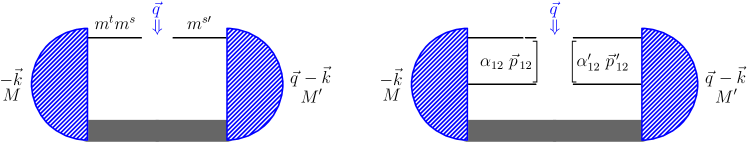
Figure 1: (Colour on-line) Sketches of the one-body (left, $n=1$) and two-body (right, $n=2$) transition probability density amplitudes, with pertinent quantum numbers and kinematics. The thick grey line denotes the $A-n$ spectator nucleons.

Specifically, the one-body density $\rho^{M^{\prime}M}_{m^{t}m_{s}^{\prime}m^{s}}(\vec{q}\mkern 2.0mu\vphantom{q})$ ($n=1$, left in fig. 1) is the transition probability density amplitude to find nucleon $A$ with specific isospin-spin projection $(m^{t}m^{s})$ inside a nucleus of momentum $-\vec{k}\mkern 2.0mu\vphantom{k}$ and spin projection $M$ in the centre-of-mass system, to have it absorb a momentum transfer $\vec{q}\mkern 2.0mu\vphantom{q}$ and re-arrange its spin projection to $m^{s\prime}$, and finally be re-incorporated into the $A$-body system such that the outgoing nucleus remains intact and in its ground state—although now with spin projection $M^{\prime}$. The one-body interaction kernel $O_{A}^{m^{t}m^{s\prime}m^{s}}(\vec{q}\mkern 2.0mu\vphantom{q})$ is then characterised by the momentum transfer $\vec{q}\mkern 2.0mu\vphantom{q}$ and the quantum numbers $(m^{t}m^{s\prime}m^{s})$, and the one-body matrix element is found by summing over them:

$$\langle\,M^{\prime}\,|\,O_{A}\,|\,M\,\rangle=\sum\limits_{\genfrac{}{}{0.0pt}{}{\scriptstyle m^{s\prime}m^{s}}{\scriptstyle m^{t}}}O_{A}^{m^{t}m^{s\prime}m^{s}}(\vec{q}\mkern 2.0mu\vphantom{q})\;\rho_{m^{t}m^{s\prime}\,m^{s}}^{M^{\prime}M}(\vec{q}\mkern 2.0mu\vphantom{q})\;\;.$$ (2.1)

To be specific and remove any ambiguity in its definition, we state that the one-body kernel is the matrix element in the specified kinematics as derived without additional factors from the (non-relativistic) Feynman rules of the pertinent process. For example, in Compton scattering, the LO [$\mathcal{O}(e^{2}\delta^{0})$] contribution is the one-nucleon Thomson term of fig. 2 (a):

$$O_{A,\,\mathrm{Thomson}}^{m^{t}m^{s\prime}m^{s}}=-\frac{(Q^{m^{t}}e)^{2}}{M_{N}}\;\vec{\epsilon}\mkern 2.0mu\vphantom{\epsilon}^{\prime\dagger}\cdot\vec{\epsilon}\mkern 2.0mu\vphantom{\epsilon}\;\delta^{m^{s\prime}m^{s}}\;\;,$$ (2.2)

with $\vec{\epsilon}\mkern 2.0mu\vphantom{\epsilon}$ and $\vec{\epsilon}\mkern 2.0mu\vphantom{\epsilon}^{\prime}$ the polarisation of the incident and outgoing photon, respectively, and $Q^{m^{t}}=m^{t}+\frac{1}{2}$ the nucleon charge in units of the elementary electric charge $e$.

Likewise, the two-body density $\rho^{M^{\prime}M}_{\alpha_{12}^{\prime}\alpha_{12}}(p_{12}^{\prime},p_{12};\vec{q}\mkern 2.0mu\vphantom{q})$ ($n=2$, right in fig. 1) is the transition probability density amplitude for the pair of nucleons $(12)$ with specific quantum numbers $\alpha_{12}$ and intrinsic relative momentum $\vec{p}\mkern 2.0mu\vphantom{p}_{12}\equiv p_{12}\;\hat{p}_{12}$ (magnitude $p_{12}$, direction $\hat{p}_{12}$) to absorb a momentum transfer $\vec{q}\mkern 2.0mu\vphantom{q}$ resulting in a new relative momentum $\vec{p}\mkern 2.0mu\vphantom{p}_{12}^{\prime}$ and new quantum numbers $\alpha^{\prime}_{12}$, before being absorbed back into the nucleus. Here, $\alpha_{12}$ is a complete set of quantum numbers which uniquely specifies the pair, including isospin $t_{12}\in\{0;1\}$ and isospin projection $m^{t}_{12}$, spin $s_{12}\in\{0;1\}$, total angular momentum $j_{12}$ with its projection $m_{12}$, and orbital angular momentum $l_{12}\in\{|j_{12}-s_{12}|;\dots;j_{12}+s_{12}\}$. The two-body kernel $O_{12}^{\alpha_{12}^{\prime}m_{12}^{s\prime}\alpha_{12}m_{12}^{s}}(\vec{p}\mkern 2.0mu\vphantom{p}_{12}^{\prime},\vec{p}\mkern 2.0mu\vphantom{p}_{12})$ is then characterised by $(\alpha_{12}^{\prime}m_{12}^{s\prime}\alpha_{12}m_{12}^{s})$ and relative momenta $(\vec{p}\mkern 2.0mu\vphantom{p}_{12}^{\prime},\vec{p}\mkern 2.0mu\vphantom{p}_{12})$. Clebsch-Gordan coefficients $\langle{j_{1}}{j_{2}}{\IfSubStr{m_{1}}{+}{(m_{1})}{\IfSubStr{m_{1}}{-}{(m_{1})}{m_{1}}}}{\IfSubStr{m_{2}}{+}{(m_{2})}{\IfSubStr{m_{2}}{-}{(m_{2})}{m_{2}}}}|{j}{\IfSubStr{m}{+}{(m)}{\IfSubStr{m}{-}{(m)}{m}}}\rangle$ in the convention of refs. [44, 45] project its angular dependence in $\vec{p}\mkern 2.0mu\vphantom{p}_{12}^{\prime}$ and $\vec{p}\mkern 2.0mu\vphantom{p}_{12}$ onto one on the orbital angular momenta $(l_{12}^{\prime},m^{l\prime}_{12})$ and $(l_{12},m^{l}_{12})$ of out- and in-states, as constrained by the spin of the nucleon pair and its total angular momentum. Hence, the additional quantum number of the spin-projection $m_{12}^{s}$ of the pair enters, too. A two-body matrix element needs finally both summation over quantum numbers and integration over the (undetected) relative momenta of the pair:

$$\begin{split}\langle&M^{\prime}\,|O_{12}|M\,\rangle\equiv\\ &\sum_{\alpha_{12}^{\prime}\alpha_{12}}\int\frac{\mathrm{d}\;\!\!p_{12}^{\prime}\;p_{12}^{\prime\,2}}{(2\pi)^{3}}\;\mathrm{d}\;\!\!p_{12}\;p_{12}^{2}\;\rho_{\alpha_{12}^{\prime}\,\alpha_{12}}^{M^{\prime}M}(p_{12}^{\prime},p_{12};\vec{q}\mkern 2.0mu\vphantom{q})\\ &\hskip 20.00003pt\times\sum_{m^{s\prime}_{12}m^{s}_{12}}\langle{l_{12}^{\prime}}{s_{12}^{\prime}}{\IfSubStr{m_{12}^{\prime}-m^{s\prime}_{12}}{+}{(m_{12}^{\prime}-m^{s\prime}_{12})}{\IfSubStr{m_{12}^{\prime}-m^{s\prime}_{12}}{-}{(m_{12}^{\prime}-m^{s\prime}_{12})}{m_{12}^{\prime}-m^{s\prime}_{12}}}}{\IfSubStr{m^{s\prime}_{12}}{+}{(m^{s\prime}_{12})}{\IfSubStr{m^{s\prime}_{12}}{-}{(m^{s\prime}_{12})}{m^{s\prime}_{12}}}}|{j_{12}^{\prime}}{\IfSubStr{m_{12}^{\prime}}{+}{(m_{12}^{\prime})}{\IfSubStr{m_{12}^{\prime}}{-}{(m_{12}^{\prime})}{m_{12}^{\prime}}}}\rangle\langle{l_{12}}{s_{12}}{\IfSubStr{m_{12}-m^{s}_{12}}{+}{(m_{12}-m^{s}_{12})}{\IfSubStr{m_{12}-m^{s}_{12}}{-}{(m_{12}-m^{s}_{12})}{m_{12}-m^{s}_{12}}}}{\IfSubStr{m^{s}_{12}}{+}{(m^{s}_{12})}{\IfSubStr{m^{s}_{12}}{-}{(m^{s}_{12})}{m^{s}_{12}}}}|{j_{12}}{\IfSubStr{m_{12}}{+}{(m_{12})}{\IfSubStr{m_{12}}{-}{(m_{12})}{m_{12}}}}\rangle\\[2.15277pt] &\hskip 20.00003pt\hskip 20.00003pt\times\int\mathrm{d}\;\!\!\hat{p}_{12}^{\prime}\;\mathrm{d}\;\!\!\hat{p}_{12}\;Y^{\dagger}_{l_{12}^{\prime}(m_{12}^{\prime}-m^{s\prime}_{12})}(\hat{p}_{12}^{\prime})\;Y_{l_{12}(m_{12}-m^{s}_{12})}(\hat{p}_{12})\;O_{12}^{\alpha_{12}^{\prime}m_{12}^{s\prime}\alpha_{12}m_{12}^{s}}(\vec{p}\mkern 2.0mu\vphantom{p}_{12}^{\,\prime},\vec{p}\mkern 2.0mu\vphantom{p}_{12};\vec{q}\mkern 2.0mu\vphantom{q})\;\;.\end{split}$$ (2.3)

In ref. [23], the integration measure $(2\pi)^{-3}$ had implicitly been attributed to the kernel but this was not explicitly stated. Since we now define the kernel as derived without additional factors from the (non-relativistic) Feynman rules of the pertinent process, this factor must be included in the convolution. To remove any such ambiguity going forward, we quote a simple contribution to the N²LO [$\mathcal{O}(e^{2}\delta^{2})$] two-body Compton kernel, namely the leftmost diagram in fig. 3 as reported first in [26] and extended to isospin $t_{12}=1$ in [27, 28, 29]:

$$O_{12,\;\mathrm{diagram\;(a)}}^{\alpha_{12}^{\prime}m_{12}^{s\prime}\alpha_{12}m_{12}^{s}}(\vec{p}\mkern 2.0mu\vphantom{p}_{12}^{\,\prime},\vec{p}\mkern 2.0mu\vphantom{p}_{12};\vec{k}\mkern 2.0mu\vphantom{k};\vec{q}\mkern 2.0mu\vphantom{q})=(-)^{t_{12}}\;\delta_{m^{t}_{12}0}\;\frac{g_{A}^{2}\;e^{2}}{2f_{\pi}^{2}}$$

$$\times\sum\limits_{\genfrac{}{}{0.0pt}{}{\scriptstyle m^{s\prime}_{1}m^{s}_{1}}{\scriptstyle m^{s\prime}_{2}m^{s}_{2}}}\langle{\frac{1}{2}}{\frac{1}{2}}{\IfSubStr{m_{1}^{s\prime}}{+}{(m_{1}^{s\prime})}{\IfSubStr{m_{1}^{s\prime}}{-}{(m_{1}^{s\prime})}{m_{1}^{s\prime}}}}{\IfSubStr{m_{2}^{s\prime}}{+}{(m_{2}^{s\prime})}{\IfSubStr{m_{2}^{s\prime}}{-}{(m_{2}^{s\prime})}{m_{2}^{s\prime}}}}|{s_{12}^{\prime}}{\IfSubStr{m_{12}^{s\prime}}{+}{(m_{12}^{s\prime})}{\IfSubStr{m_{12}^{s\prime}}{-}{(m_{12}^{s\prime})}{m_{12}^{s\prime}}}}\rangle\,\langle{\frac{1}{2}}{\frac{1}{2}}{\IfSubStr{m_{1}^{s}}{+}{(m_{1}^{s})}{\IfSubStr{m_{1}^{s}}{-}{(m_{1}^{s})}{m_{1}^{s}}}}{\IfSubStr{m_{2}^{s}}{+}{(m_{2}^{s})}{\IfSubStr{m_{2}^{s}}{-}{(m_{2}^{s})}{m_{2}^{s}}}}|{s_{12}}{\IfSubStr{m_{12}^{s}}{+}{(m_{12}^{s})}{\IfSubStr{m_{12}^{s}}{-}{(m_{12}^{s})}{m_{12}^{s}}}}\rangle\;\frac{\vec{\epsilon}\mkern 2.0mu\vphantom{\epsilon}\cdot(\vec{\sigma}\mkern 2.0mu\vphantom{\sigma}_{1})^{m^{s\prime}_{1}}{}_{m^{s}_{1}}\;\vec{\epsilon}\mkern 2.0mu\vphantom{\epsilon}^{\prime\dagger}\cdot(\vec{\sigma}\mkern 2.0mu\vphantom{\sigma}_{2})^{m^{s\prime}_{2}}{}_{m^{s}_{2}}}{\omega^{2}-m_{\pi}^{2}-(\vec{p}\mkern 2.0mu\vphantom{p}_{12}-\vec{p}\mkern 2.0mu\vphantom{p}_{12}^{\prime}+\vec{k}\mkern 2.0mu\vphantom{k}+\frac{\vec{q}\mkern 2.0mu\vphantom{q}}{2})^{2}}+(1\leftrightarrow 2)\;\;.$$

Here, $g_{A}=1.267$ is the pion-nucleon coupling, $f_{\pi}=92.42\;\mathrm{MeV}$ the pion decay constant, $m_{\pi}=139.5675\;\mathrm{MeV}$ its mass, $(\omega,\vec{k}\mkern 2.0mu\vphantom{k})$ the incident photon’s $4$-momentum, and $(\vec{\sigma}\mkern 2.0mu\vphantom{\sigma}_{i})^{m^{s\prime}_{i}}{}_{m^{s}_{i}}$ the components of the Pauli spin matrix of nucleon $i$ which combine to a given $s_{12}$ and $m_{12}^{s}$. As customary, $(1\leftrightarrow 2)$ stands for another term with the rôles of the nucleons exchanged, $\vec{p}\mkern 2.0mu\vphantom{p}_{12}\to-\vec{p}\mkern 2.0mu\vphantom{p}_{12}$, $\vec{p}\mkern 2.0mu\vphantom{p}_{12}^{\prime}\to-\vec{p}\mkern 2.0mu\vphantom{p}_{12}^{\prime}$, and with $t_{12}+l_{12}+s_{12}$ odd due to the Pauli principle.

At zero momentum transfer, the trace of each one- or two-body density in the space of quantum numbers and momenta is normalised to $1$ (i.e. one nucleon or one nucleon-pair is active); see [23] for details and symmetry properties.

Before closing this section, we note that the probabilistic interpretation of an $n$-body transition density amplitude we laid out here is only rigorously true to the extent that a $n$-body operator can be used to compute the probability amplitude; cf. some popular and recent accounts [46, 47, 48]. At momenta of order $\overline{\Lambda}_{\chi}$, dependence on the chiral interactions and on phenomena at momenta above the domain of $\chi$EFT enter each $n$-body transition density amplitude. In observables, these are compensated for by other operators involving different $m\neq n$-body densities as well as higher-order effects in both the kernel and potential. For example, high-momentum parts of one-body densities play against those of two-body densities. That makes a simple physical interpretation of the Transition Density along the lines of this subsection inaccurate at such momenta.

2.2 Compton Observables in ⁴He

In addition to the quantum numbers of the active nucleons, Compton scattering is characterised by the quantum numbers of the photons: initial and final polarisations $\lambda,\lambda^{\prime}$. The total matrix element is finally obtained by weighting with the number of indistinguishable nucleons and nucleon pairs,

$$A_{M\lambda}^{M^{\prime}\lambda^{\prime}}(\vec{k}\mkern 2.0mu\vphantom{k},\vec{q}\mkern 2.0mu\vphantom{q})=\genfrac{(}{)}{0.0pt}{}{A}{1}\;\langle M^{\prime}|{O}^{\lambda^{\prime}\lambda}_{A}|M\rangle\;+\;\genfrac{(}{)}{0.0pt}{}{A}{2}\;\langle M^{\prime}|{O}^{\lambda^{\prime}\lambda}_{12}|M\rangle\;+\;\dots\;\;,$$ (2.5)

with $A=4$ nucleons inside ⁴He. The ellipses denote more-body kernels which are of higher order, as discussed in sect. 2.3. This amplitude is evaluated in the cm frame of the photon-nucleus system, where no energy is transferred. In Compton scattering, the momentum-transfer $\vec{q}\mkern 2.0mu\vphantom{q}$ which characterises the transition densities is traditionally replaced by the energy of both incident and outgoing photon, $\omega_{\mathrm{cm}}=|\vec{k}\mkern 2.0mu\vphantom{k}|=|\vec{k}\mkern 2.0mu\vphantom{k}^{\prime}|$ and by the scattering angle $\theta_{\mathrm{cm}}$ for the outgoing photon:

$$\cos\theta_{\mathrm{cm}}=1-\frac{\vec{q}\mkern 2.0mu\vphantom{q}^{\,2}}{2\omega_{\mathrm{cm}}^{2}}\;\;.$$ (2.6)

The ⁴He Compton cross section (target spin $0$, i.e. $M^{\prime}=M=0$) in the lab frame is finally found by transferring angles and energies from the cm using the ⁴He mass of $3727.4\;\mathrm{MeV}$ and averaging (summing) over initial (final) photon polarisations:

$$\frac{\mathrm{d}\sigma}{\mathrm{d}\Omega}=\frac{1}{2}\left(\frac{\omega_{\mathrm{lab}}^{\prime}}{4\pi\omega_{\mathrm{lab}}}\right)^{2}\sum\limits_{\lambda^{\prime}\lambda}\left|A_{0\lambda}^{0\lambda^{\prime}}(\vec{k}\mkern 2.0mu\vphantom{k},\vec{q}\mkern 2.0mu\vphantom{q})\right|^{2}\;\;.$$ (2.7)

In (elastic) Compton scattering on a spin-$0$ target like ⁴He, only one more observable is realistically measurable in today’s facilities: the asymmetry of a linearly polarised beam without measurement of the scattered photon’s polarisation:

$$\Sigma^{\text{lin}}\equiv\Sigma_{3}:=\frac{\mathrm{d}\sigma^{||}-\mathrm{d}\sigma^{\perp}}{\mathrm{d}\sigma^{||}+\mathrm{d}\sigma^{\perp}}=-\frac{\sum\limits_{\lambda^{\prime}\lambda}A_{0\lambda}^{0\lambda^{\prime}}(\vec{k}\mkern 2.0mu\vphantom{k},\vec{q}\mkern 2.0mu\vphantom{q})\;[A_{0-\lambda}^{0\lambda^{\prime}}(\vec{k}\mkern 2.0mu\vphantom{k},\vec{q}\mkern 2.0mu\vphantom{q})]^{\dagger}}{\sum\limits_{\lambda^{\prime}\lambda}\left|A_{0\lambda}^{0\lambda^{\prime}}(\vec{k}\mkern 2.0mu\vphantom{k},\vec{q}\mkern 2.0mu\vphantom{q})\right|^{2}}\;\;.$$ (2.8)

Here, $\mathrm{d}\sigma$ is shorthand for ${\mathrm{d}\sigma}/{\mathrm{d}\Omega}$ and superscripts refer to photon polarisations (“$\parallel$” for polarisation in the scattering plane, “$\perp$” for perpendicular to it). The kinematic variables must of course be transferred to the lab frame as appropriate.

2.3 Compton Kernel

For reviews of Compton scattering on nucleons and light nuclei in $\chi$EFT, we refer the reader to refs. [2, 49] for notation, relevant parts of the chiral Lagrangian, and full references to the literature. Here, we merely summarise the power counting and Compton kernel already employed in refs. [50, 51, 25] in our region of interest, $50\;\mathrm{MeV}\lesssim\omega\lesssim 120\;\mathrm{MeV}$.

When $\chi$EFT with a dynamical Delta is used to compute (elastic) Compton scattering, three low scales compete: the pion mass $m_{\pi}$, the Delta-nucleon mass splitting $\Delta_{\scriptscriptstyle M}\approx 300\;\mathrm{MeV}$, and the photon energy $\omega$. Each provides a small, dimensionless expansion parameter, measured in units of the “high” momentum scale $\overline{\Lambda}_{\chi}$, at which the theory breaks down because new degrees of freedom enter. While $\frac{m_{\pi}}{\overline{\Lambda}_{\chi}}$ and $\frac{\Delta_{\scriptscriptstyle M}}{\overline{\Lambda}_{\chi}}$ have quite different chiral behaviour, we follow Pascalutsa and Phillips [54] and take a common breakdown scale $\overline{\Lambda}_{\chi}\approx 650\;\mathrm{MeV}$, consistent with the masses of the $\omega$ and $\rho$ as the next-lightest exchange mesons, exploiting a numerical coincidence at the physical pion mass to define a single expansion parameter:

$$\delta\equiv\frac{\Delta_{M}}{\overline{\Lambda}_{\chi}}\approx\sqrt{\frac{m_{\pi}}{\overline{\Lambda}_{\chi}}}\approx\sqrt{\frac{\omega}{\overline{\Lambda}_{\chi}}}\approx 0.4\ll 1\;\;.$$ (2.9)

We also count $M_{\mathrm{N}}\sim\overline{\Lambda}_{\chi}$. Since $\delta$ is not very small, order-by-order convergence must be verified carefully, see sect. 3.3.

This power counting organises contributions under the assumption $\omega\sim m_{\pi}$. As extensively discussed previously [26, 55, 50, 51, 25] and summarised in [2, sect. 5.2], in this régime only kernels with one and two active nucleons contribute in a $\chi$EFT description of Compton scattering up to and including N⁴LO [$\mathcal{O}(e^{2}\delta^{4})$]. At lower energies $\omega\lesssim m_{\pi}^{2}/M$, this power counting does not apply because photons with resolution $1/\omega$ larger than the size of the ⁴He nucleus scatter coherently on the whole target. Refs. [50, 51, 2] discuss in detail how the reformulated power counting appropriate at these lower energies leads to the restoration of the Thomson limit by inclusion of coherent propagation of the ⁴He system in the intermediate state between absorption and emission of photons. This rescattering effect involves the interaction of all $A$ nucleons with one another between photon absorption and emission, and hence an $A$-body density. However, that régime is not the focus of this presentation. Rather, we are concerned with the non-collective contributions which dominate above about $50\;\mathrm{MeV}$. That is also where data is most likely to be taken to extract nucleon polarisabilities.

Specifically, we use the one- and two-body Compton kernels of refs. [56, 57, 26], supplemented with the $\Delta$-pole and $\pi\Delta$ loop graphs [58, 59, 50, 51]. They are both conceptually and numerically identical to the ones which have been described extensively in our Compton studies of the deuteron [50, 51, 60, 3, 4] and, most recently, ³He [25, 23]. These pieces of the photonuclear operator are organised in a perturbative expansion which is complete up to and including N³LO [$\mathcal{O}(e^{2}\delta^{3})$]. No contribution enters at NLO [$\mathcal{O}(e^{2}\delta^{1})$], and only one-body Delta contributions at N³LO [$\mathcal{O}(e^{2}\delta^{3})$]. We only allow photon energies somewhat below $\omega_{\mathrm{thr}}(\mbox{${}^{4}$He})\approx m_{\pi}$ in order to avoid additional complications in the vicinity of the pion-production threshold.

The one-nucleon kernel convoluted with the one-body density as in eq. (2.1) is sketched in fig. 2:

• LO [$\mathcal{O}(e^{2}\delta^{0}=Q^{2})$]: The single-nucleon (proton) Thomson term.

• N²LO [$\mathcal{O}(e^{2}\delta^{2}=Q^{3})$] non-structure/Born terms: photon couplings to the nucleon charge beyond LO, to its magnetic moment, or to the $t$-channel exchange of a $\pi^{0}$ meson (irrelevant for the isoscalar ⁴He).

• N²LO [$\mathcal{O}(e^{2}\delta^{2}=Q^{3})$] structure/non-Born terms: photon couplings to the pion cloud around the nucleon is the source of the LO contributions to the polarisabilities as first reported in refs. [56, 57].

• N³LO [$\mathcal{O}(e^{2}\delta^{3})$] structure/non-Born terms: photon couplings to the pion cloud around the (non-relativistic) $\Delta(1232)$ (d) or directly exciting the Delta (e), as calculated in refs. [61, 62, 63]; these give NLO contributions to the polarisabilities. The Delta parameters are taken from ref. [25]. The Delta excitation of diagram (d) shows considerable energy dependence even at $\omega\sim m_{\pi}$; see the discussion of “dynamical polarisabilities” in refs. [2, 64]. This will be important in the interpretation of our results in sect. 3.

• Short-distance/low-energy coefficients (LECs) encode those contributions to the nucleon polarisabilities which stem from physics at and above the breakdown scale $\overline{\Lambda}_{\chi}$. These offsets to the polarisabilities are formally of higher order. We determine them to reproduce the isoscalar polarisabilities of eq. (1.1). Their uncertainties were discussed in the Introduction but are dwarfed by the other uncertainties of the results presented here, including those coming from the wave function dependence and higher order effects; see sect. 3.3. Neither does the detailed discussion of the sources and sizes of uncertainties of other nucleon polarisabilities in ref. [5] bear on the present results. We also recall from the Introduction that since ⁴He is a near-perfect isoscalar and scalar, neither the nucleon’s isovector polarisabilities nor its spin polarisabilities enter, except at very high orders.

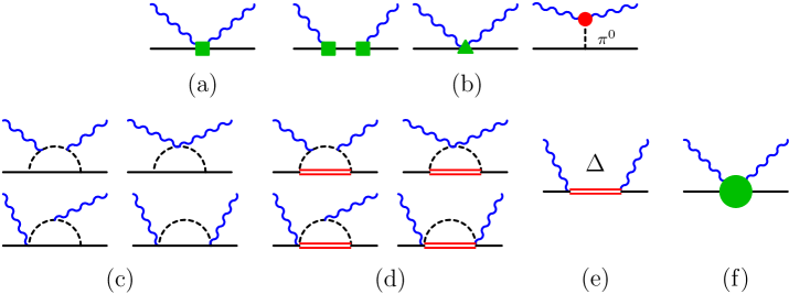
Figure 2: (Colour on-line) The single-nucleon contributions in $\chi$EFT up to N³LO [$\mathcal{O}(e^{2}\delta^{3})$] for $50\;\mathrm{MeV}\lesssim\omega\lesssim 120\;\mathrm{MeV}$. The vertices are from: ${\cal L}_{\pi\mathrm{N}}^{(1)}$ (no symbol), ${\cal L}_{\pi\mathrm{N}}^{(2)}$ (green square), ${\cal L}_{\pi\mathrm{N}}^{(3)}$ (green triangle), ${\cal L}_{\pi\pi}^{(4)}$ (red disc) [57]; the green disc of graph (f) stands for variations of the polarisabilities. Permuted and crossed diagrams are not displayed.

Figure 3: (Colour on-line) N²LO [$\mathcal{O}(e^{2}\delta^{2})$] contributions to the (irreducible) $\gamma\mathrm{N}\mathrm{N}\rightarrow\gamma\mathrm{N}\mathrm{N}$ amplitude (no additional contributions at N³LO [$\mathcal{O}(e^{2}\delta^{3})$]. Notation as in fig. 2. Permuted and crossed diagrams not displayed.

The first nonzero two-body kernel convoluted with the two-body density as in eq. (2.3) enters at N²LO [$\mathcal{O}(e^{2}\delta^{2})$] and does not involve Delta excitations; see fig. 3. It is the two-body analogue of the $\pi N$ loop graphs (c) in fig. 2, first computed for $t_{12}=0$ in refs. [26, 55] and extended to $t_{12}=1$ in refs. [27, 28, 29] where full expressions can be found. These contributions are nonzero only for $\mathrm{np}$ pairs, i.e. they all contain the same $2\mathrm{N}$ isospin factor of eq. (2.1):

$$\langle t_{12}m^{t\prime}_{12}|(\tau^{(1)}\cdot\tau^{(2)}-\tau^{(1)}_{z}\tau^{(2)}_{z})|t_{12}m^{t}_{12}\rangle=2(-)^{t_{12}+1}\;\delta_{m^{t\prime}_{12}m^{t}_{12}}\;\delta_{m^{t}_{12}0}\;\;.$$ (2.10)

Therefore, they parametrise the leading term of both photons hitting the charged-meson-exchange. In ⁴He, as in ³He, both isospin $t_{12}=0$ and $1$ pairs are present. Corrections to these currents enter at one order higher, N⁴LO [$\mathcal{O}(e^{2}\delta^{4})$], than we consider here.

2.4 Generation of Transition Densities from Potentials

We used a class of four chiral $2$N and $3$N interactions to generate the one- and two-body densities for ⁴He: the $\chi$EFT Semi-local Momentum-Space (SMS) $2\mathrm{N}$ potentials in the version “N⁴LO +” (i.e. considered to be complete at N⁴LO with some N⁵LO interactions) [65] and the corresponding chiral $3\mathrm{N}$ interaction “N²LO” discussed in ref. [66]. We employed $2\mathrm{N}$ momentum-space cutoffs $\Lambda=550\;\mathrm{MeV}$ (hardest), $500\;\mathrm{MeV}$, $450\;\mathrm{MeV}$ and $400\;\mathrm{MeV}$ (softest) (the complete set of parameters of the 3N interactions can be found in Table 1 of Ref. [67]). These nuclear interactions all capture the correct long-distance physics of one- and two-pion exchange and reproduce both the $2\mathrm{N}$ scattering data and the experimental values of the triton and ³He binding energies well. Increasing momentum cutoffs indicate increasing “hardness” of the short-distance interaction. Their ⁴He binding energies are within $+0.5\;\mathrm{MeV}$ ($\Lambda=550\;\mathrm{MeV}$) to $-0.1\;\mathrm{MeV}$ ($\Lambda=400\;\mathrm{MeV}$) of the experimental value. This variation by less than $2\%$ is not a concern, since we compute for photon energies that are high enough that this slight variation in the ⁴He binding energy has no impact on the elastic Compton cross section.

These are of course but four out of a number of modern, sophisticated potentials. Our choice is dictated by the fact that they are semi-local (and hence of the form of AV18) and are already coded for the densities formalism. By varying the cutoff within a single family of $\chi$EFT potentials, we avoid questions about how the cutoffs of different realisations of the $\chi$EFT regulator functions are related. The range of cutoffs chosen, while not large enough to establish renormalisability of the theory, is large enough to indicate a lower bound of the sensitivity of cross sections to the short-distance physics of this process.

These $\chi$EFT wave functions use Weinberg’s “hybrid approach” [33], in which potentials are derived to an assumed accuracy and then iterated to produce amplitudes or, in our case, one- and two-body densities. All claim a higher accuracy than that of our Compton kernels. We refrain here from entering the ongoing debate about correct implementations of the chiral power counting or the range of cutoff variations, etc.; see refs. [68, 69] for concise summaries, ref. [53] for a polemic, and ref. [70] for a variety of community voices.

Similarly, even though the Compton Ward identities are violated because the one-pion-exchange $2\mathrm{N}$ potentials are regulated, any inconsistencies between currents and nuclear densities is compensated by operators which enter at higher orders in $\chi$EFT than the last order we fully retain [N³LO, $\mathcal{O}(e^{2}\delta^{3})$]. In addition, the potentials do not include explicit Delta contributions while the kernel does. However, it is easy to see that, for real Compton scattering around $120\;\mathrm{MeV}$, a Delta excited directly by the incoming photon is more important than one that occurs virtually between exchanges of virtual pions, especially for an isoscalar target like ⁴He. For our purposes, such Delta excitations in the $2\mathrm{N}$ potential are already suppressed by several orders in the chiral counting and well approximated by the $\pi N$ seagull Low Energy Coefficients that enter the N³LO interaction.

In sect. 3.3.3, we therefore take the differences between results with the $4$ different sets of densities as providing a lower bound indicative of the present residual theoretical uncertainties. These do not affect the conclusions of our sensitivity studies, but better extractions of polarisabilities from ⁴He data will undoubtedly need a reduced potential spread. The results generated with the potential $\chi$SMSN⁴LO+$450\mathrm{MeV}$+N²LO3NI turn out to be approximately the mean of those generated from the different potentials considered, so we use that for central values, and assess variations with respect to it.

The ⁴He one- and two-body densities, together with the ³He densities, are publicly available using the python package provided at https://pypi.org/project/nucdens/. They are defined in momentum space, for centre-of-mass energies and momentum transfers corresponding to Compton scattering photon energies between $\omega_{\mathrm{cm}}=50$ and $120\;\mathrm{MeV}$ in steps of $10\;\mathrm{MeV}$ and scattering angles $\theta_{\mathrm{cm}}\in[0;180^{\circ}]$ in steps of $15^{\circ}$ (momentum-transfers $\sqrt{\vec{q}\mkern 2.0mu\vphantom{q}^{2}}\in[0;240]\;\mathrm{MeV}$), plus at selected higher and lower energies for control. Also available are densities using the harder AV18 $2\mathrm{N}$ model interaction [71], supplemented by the Urbana-IX $3\mathrm{N}$ interaction (3NI) [72, 73], and densities using the chiral Idaho interaction for the $2\mathrm{N}$ system in the version “N³LO” at cutoff $500\;\mathrm{MeV}$ [74] with the $\chi$EFT $3\mathrm{N}$ interaction in the version “$\mathcal{O}(Q^{3})$” using variant “b” of ref. [75] as the “softest” choice.

3 Results

3.1 Overview and Main Result

Figure 4 summarises our key result, on which we elaborate in the subsequent sub-sections. $\chi$EFT agrees well with the available data for $\omega_{\mathrm{cm}}\gtrsim 50\;\mathrm{MeV}$, as we explain in detail in sect. 3.2. In sect. 3.3, we demonstrate that the $\chi$EFT treatment of Compton scattering on ⁴He at N³LO [$\mathcal{O}(e^{2}\delta^{3})$] has $\lesssim\pm 10\%$ uncertainties from the dependence on the $2\mathrm{N}$ and $3\mathrm{N}$ interactions employed and from an assessment of order-by-order convergence of the EFT.

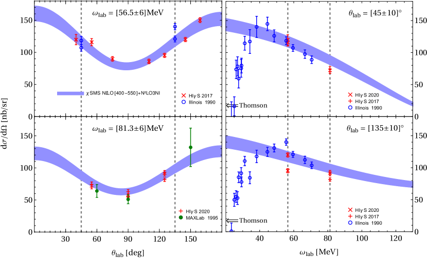
Figure 4: (Colour on-line) The band of the differential cross sections at N³LO [$\mathcal{O}(e^{2}\delta^{3})$] mapped out by results generated using the nucleon densities from four $\chi$SMSN⁴LO +N²LO3NI potentials with cutoffs $\{400;450;500;550\}\;\mathrm{MeV}$, at $\omega_{\mathrm{lab}}=56.5\;\mathrm{MeV}$ (top left) and $81.3\;\mathrm{MeV}$ (bottom left), and angles $\theta_{\mathrm{lab}}=45^{\circ}$ (top right) and $135^{\circ}$ (bottom right). All the data from Illinois [76], MAXlab [77] and two HI$\gamma$S runs [21, 78] are included, via the ranges indicated in each plot. (The small effect of the difference between nominal and actual energies or angles is not accounted for here; see sect. 3.2 for details.) Vertical dashed lines in the $\omega_{\mathrm{lab}}$ plots (left) correspond to the angles in the $\theta_{\mathrm{lab}}$ plots (right), and vice versa. On the right, arrows at $20\;\mathrm{MeV}$ indicate the Thomson limit ($\omega=0$) at given $\theta$. The disagreement between theory and experiment for $\omega_{\mathrm{lab}}\lesssim 50\;\mathrm{MeV}$ is expected; see text for details.

Figure 5 shows that the cross section drops steadily with energy. Concurrently, it starts out almost fore-back symmetric but becomes quite lopsided as scattering under backward angles grows relative to forward angles. At $120\;\mathrm{MeV}$, back-angle cross sections are about twice as big as forward-angle ones and have reduced to a bit more than half of their $\omega_{\mathrm{lab}}=50\;\mathrm{MeV}$ values. This is consistent with findings for the deuteron and ³He [59, 50, 51, 60, 25], although there the fore-aft asymmetry is with only about $1:1.2$ not nearly as dramatic.

We analyse the sensitivity to the scalar-isoscalar dipole polarisabilities of the nucleon in sect. 3.4. We will concentrate on three energies $\{60;90;120\}\;\mathrm{MeV}$ to cover the possible range of future experiments. For these, the subsequent figures 6 to 8 at $\{45^{\circ};120^{\circ};150^{\circ}\}$ display the energy dependence of our results. We consider these to provide a good compromise between experimental feasibility and valuable information on the polarisabilities. In sect. 3.5, the beam asymmetry’s convergence and sensitivity to $\alpha_{E1}^{(\mathrm{s})}$ and $\beta_{M1}^{(\mathrm{s})}$ is addressed.

Throughout secs. 3.3 to 3.5 we assess the difference between two quantities (e.g. the cross section using two different potentials) by defining:

$$\mbox{``relative deviation of $A$ from $M$'' }:=\frac{A}{M}-1\;\;.$$ (3.1)

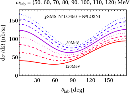
Figure 5: (Colour on-line) Evolution of the differential ⁴He Compton cross section at N³LO [$\mathcal{O}(e^{2}\delta^{3})$], in the lab frame from $50$ (top) to $120\;\mathrm{MeV}$ (bottom) in steps of $10\;\mathrm{MeV}$, for densities generated using the “mean” potential $\chi$SMSN⁴LO+$450\mathrm{MeV}$+N²LO3NI.

3.2 Comparison with Data

A total of $50$ measurements are available. Those with the highest precision come from HI$\gamma$S using a quasi-monchromatic photon beam: $7$ points at $56.5\;\mathrm{MeV}$ published in 2017 [21], and another $8$ at $81.3\;\mathrm{MeV}$ published in 2020 [78]. Older data are available from two tagged-photon bremsstrahlung facilities: $3$ points from MAXlab at $87\;\mathrm{MeV}$ in 1995 [77]; and the largest dataset, $32$ points, from the University of Illinois Tagged Photon Facility between $23.4\;\mathrm{MeV}$ and $70.55\;\mathrm{MeV}$ at $45^{\circ}$ and $135^{\circ}$ [76]. This pioneering set from 1990 covers the widest energy range, but also carries the largest uncertainties. We present the data with error bars which add statistical and point-to-point systematic uncertainties in quadrature but which do not account for systematic correlated/overall uncertainties. These are reported as $2.2\%$ for both HI$\gamma$S sets, $15\%$ for the MAXlab set, but not reported for the Illinois set.

To compare these data with our result in fig. 4, we chose $4$ fixed-energy and fixed-angle slices in which each datum is represented at least once: two fixed-energy plots at the energies of the HI$\gamma$S data, $56.5\;\mathrm{MeV}$ and $81\;\mathrm{MeV}$, but containing also data within $\pm 6\;\mathrm{MeV}$ of the central values; and two fixed-angle plots at the angles of the Illinois data—$45^{\circ}$ and $135^{\circ}$—but including data within $\pm 10^{\circ}$. Cognisant of the present accuracies of both data and theory, we do not correct cross sections of data whose energy or scattering angle do not exactly match the central values; the differences are visible but smaller than even the experimental error bars. The Illinois data for $56.5\;\mathrm{MeV}$ at back-angles appear somewhat higher than the HI$\gamma$S ones, while all are consistent at forward angles. At $81.3\;\mathrm{MeV}$, all data appear to be consistent. At fixed angles, the Illinois set appears to be slightly more sloped as a function of energy than the HI$\gamma$S data and the theory curve. It may, however, be worth recalling that the Illinois data were obtained at a first-generation tagged-photon facility.

Agreement of theory and data is good within the experimental and theoretical uncertainties in the range where the assumptions of the present theoretical description hold: namely for those $\omega\sim m_{\pi}$ for which the intermediate four-nucleon system predominantly propagates incoherently, with only minor effects from restoring the Thomson limit, as discussed in sect. 2.3. At $\omega\lesssim 50\;\mathrm{MeV}$, the only data are from Illinois [76]. They show a rapid drop towards the Thomson limit after a “knee” around $40$ to $50\;\mathrm{MeV}$. These data at the lowest energies are not inconsistent with the Thomson limit (denoted by arrows at $20\;\mathrm{MeV}$ in the energy-dependent plots). Informed by these comparisons and accounting for the uncertainties of both theory and experiment, we conclude that the incoherent-propagation assumption is justified for $\omega\gtrsim 50\;\mathrm{MeV}$, consistent with the a-priori estimate of sect. 3.3.1.

To put their HI$\gamma$S data in context, Sikora et al.  used a phenomenological model to parametrise the ⁴He elastic Compton cross section [21]. In it, the density of nucleons is captured as a Fermi function; photons interact with the nucleons through one-body $E1,E1$ and $M1,M1$ operators; and two-body currents are included so that they provide the right overall strength. Sikora et al.’s isoscalar polarisability values of $10.9$ and $3.6$ are close to the numbers employed here. Crucially though, the one-body amplitude does not include dispersive effects in $\alpha_{E1}$ and $\beta_{M1}$. However, the energy dependence of these polarisabilities is known to be a crucial effect for photon energies approaching $100\;\mathrm{MeV}$ [58, 50, 51, 2]; this is likely responsible for the disagreement between this model and their data. In addition, it has been demonstrated that higher photon multipoles are relevant at such energies in the $\gamma$-deuteron reaction [50, 51]. All this stems from the fact that Sikora et al.’s model does not account for the pion dynamics in either the polarisabilities or the exchange currents, and so lacks a microscopic description of the energy dependence of the former and the size of the latter. In contrast, our $\chi$EFT calculation predicts both of these effects via a consistent underlying theory. It also delivers a much more accurate treatment of the ⁴He wave function.

The systematic nature of the $\chi$EFT expansion means that we can estimate the uncertainties induced by truncating its $\gamma{}^{4}$He amplitude at N³LO [$\mathcal{O}(e^{2}\delta^{3})]$—something that is required for a rigorous comparison between $\chi$EFT and these data. We will discuss in the next subsection how that uncertainty estimate produces the bands in fig. 4.

3.3 Theoretical Uncertainties

As in previous presentations on Compton scattering on the deuteron [2, 5] and ³He [25], we assess convergence and theoretical uncertainties in three ways, each based on the $\chi$EFT expansion: a-priori; order-by-order; and residual dependence on short-distance details. As described in sect. 2.3, the Compton kernel is incomplete at low energies, $\omega\lesssim 50\;\mathrm{MeV}$ because rescattering contributions become important and finally restore the correct Thomson limit as $\omega\to 0$. Thus, the estimates we are about to discuss do not apply there.

We reiterate that our results are exploratory and do not yet suffice for high-accuracy extractions of polarisabilities from data. For that, the Thomson limit should be restored. This should also reduce the dependence on the $2\mathrm{N}$ and $3\mathrm{N}$ interaction. Therefore, we do not explore a rigorous interpretation of theoretical uncertainties based on Bayesian statistics as developed in [79, 5, 80, 81].

3.3.1 A-Priori Estimate

For the a-priori estimate, the Compton amplitudes are complete up to and including N³LO [$\mathcal{O}(e^{2}\delta^{3})$] and therefore carry an uncertainty of roughly $\delta^{4}\approx(0.4)^{4}\approx\pm 3\%$ of the LO result. This translates into about $\pm 6\%$ for cross sections and beam asymmetries since these are proportional to the square of amplitudes. This appears to be a slight under-estimate when placed alongside the following two post-facto criteria, but the contribution at any EFT order is always multiplied by a number of order one, and there is also some uncertainty in the breakdown scale.

3.3.2 Convergence of the $\chi$EFT Expansion

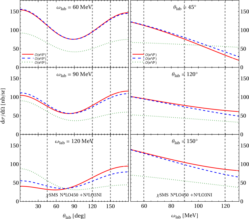
Figure 6: (Colour on-line) The cross section at N³LO [$\mathcal{O}(e^{2}\delta^{3})$] (with Delta; red solid), N²LO [$\mathcal{O}(e^{2}\delta^{2})$] (no Delta; blue dashed), and LO [$\mathcal{O}(e^{2}\delta^{0})$] (single-nucleon Thomson term only; green dotted), using the “mean” potential $\chi$SMSN⁴LO+$450\mathrm{MeV}$+N²LO3NI; see text for details. Vertical dashed lines in the $\omega_{\mathrm{lab}}$ plots (left) correspond to the angles in the $\theta_{\mathrm{lab}}$ plots (right), and vice versa.

The second assessment uses order-by-order convergence. So that differences between the orders are not contaminated by spurious dependencies, we use the same values for the static nucleon polarisabilities at both N²LO [$\mathcal{O}(e^{2}\delta^{2})$] and N³LO [$\mathcal{O}(e^{2}\delta^{3})$] (no polarisabilities enter at LO [$\mathcal{O}(e^{2}\delta^{0})$]). We notice that the sensitivity of observables to varying polarisabilities is for all practical purposes unaffected by the exact choice of their central values.

As fig. 6 shows, the correction from $\mathcal{O}(e^{2}\delta^{2})$ [N²LO, i.e. without the Delta] to $\mathcal{O}(e^{2}\delta^{3})$ [N³LO, i.e. including the Delta] is indeed smaller than that from $\mathcal{O}(e^{2}\delta^{0})$ [LO] to $\mathcal{O}(e^{2}\delta^{2})$ [N²LO ]; remember that there is no correction at $\mathcal{O}(e^{2}\delta^{1})$ [NLO]. That the LO-to-N²LO correction is generally quite large in Compton scattering has already been observed for the nucleon, deuteron, and ³He [25]. After all, LO is just the Thomson term for the proton, and the contributions from charged-pion-exchange currents are significant in the deuteron and ³He [59, 50, 51, 60, 25]. While a correction of about $50\%$ at $60\;\mathrm{MeV}$ is similar to that in ³He [25], the correction of about $50\%$ at $120\;\mathrm{MeV}$ is smaller than the $\lesssim 70\%$ correction in ³He, especially at forward angles. This can be explained by a combination of effects. First, ⁴He is more tightly bound and hence smaller. Second, and perhaps more important, in the isospinor target ³He, both the rather small isoscalar magnetic moment $\mu^{(\mathrm{s})}\approx 0.43$ and the much larger isovector piece $\mu^{(\mathrm{v})}\approx 4.7$ contributes. Since ⁴He is isoscalar, so the latter is absent at the order we consider. Overall, the size of the LO-to-N²LO correction is a poor predictor for the typical size of higher-order terms. We will not use it to estimate uncertainties based on convergence.

On the other hand, the correction from $\mathcal{O}(e^{2}\delta^{2})$ [N²LO ] to $\mathcal{O}(e^{2}\delta^{3})$ [N³LO ] becomes visible only at energies above about $80\;\mathrm{MeV}$. This is not entirely surprising since the additional pieces contain the $\Delta(1232)$ whose effect beyond that on the static polarisabilities is constrained be small at low energies. Further charged-meson-exchange contributions at N⁴LO will shed more light on whether such a small shift is accidental. Towards $120\;\mathrm{MeV}$, the $\Delta(1232)$’s effect changes the angle dependence significantly, reducing forward scattering by about $35\%$ while increasing back-scattering by about $20\%$. That is consistent with the findings in the deuteron and ³He [50, 51, 60, 25]. It might at first be surprising that the $\Delta(1232)$ has such a large effect well below its resonance threshold. However, ref. [25] already pointed out that while the static magnetic polarisability $\beta_{M1}^{(\mathrm{s})}$ is by construction unchanged between orders, the $\Delta(1232)$ adds a sizeable dispersive correction which can be as large as the static value of $\beta_{M1}^{(\mathrm{s})}$ itself; see the discussion of “dynamical polarisabilities” in refs. [2, 64].

Taking all his into consideration, we take about $\delta\approx 0.4$ of the difference between N²LO and N³LO itself as total width of the uncertainty band from higher-order corrections. That amounts to just a per-cent at $\omega\approx 60\;\mathrm{MeV}$, which is clearly an under-estimate also in view of the a-priori estimate above. It increases for $120\;\mathrm{MeV}$ to about $\pm 8\%$ forward and about $\pm 4\%$ backward, or some $\pm 6\%$ overall.

3.3.3 Residual Dependence on the $2\mathrm{N}$ and $3\mathrm{N}$ Interactions

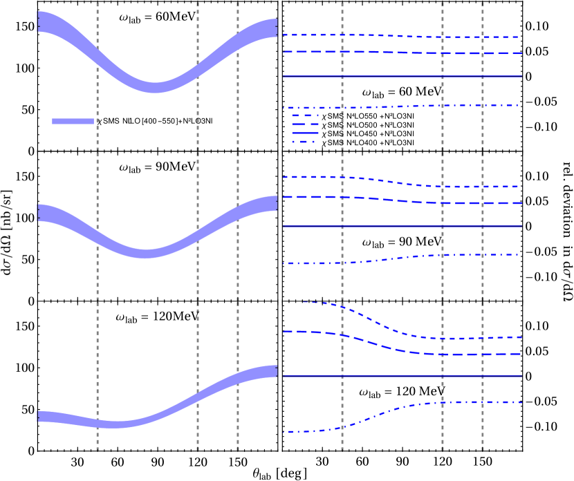
Figure 7: (Colour on-line) Energy- and angle-dependence of the four $\chi$SMSN⁴LO +N²LO3NI potentials with cutoffs $\{400;450;500;550\}\;\mathrm{MeV}$ at N³LO [$\mathcal{O}(e^{2}\delta^{3})$]. Left: spread of the potentials. Right: relative difference of each potential to a “mean” potential $\chi$SMSN⁴LO+$450\mathrm{MeV}$+N²LO3NI at N³LO [$\mathcal{O}(e^{2}\delta^{3})$]; see text for details. In both panels, vertical dashed lines denote the angles $\theta_{\mathrm{lab}}=\{45^{\circ};120^{\circ};150^{\circ}\}$ of fig. 6.

As discussed in sect. 2.4, the $\chi$SMSN⁴LO +N²LO3NI $2\mathrm{N}$ and $3\mathrm{N}$ potentials used to produce the one- and two-body densities all capture the correct long-range physics of one- and two-pion exchange and reproduce the two-nucleon scattering data and the ³He and ⁴He binding energies equally well—indeed, at a level superior to the accuracy aimed for in this article. Therefore, differences only stem from the different cutoffs $\{400;450;500;550\}\;\mathrm{MeV}$, i.e. from short-range dynamics not explicitly included in $\chi$EFT. Those differences therefore provide an estimate of the effect of higher-order terms in the $\chi$EFT series. This estimate provides a lower bound of the theoretical uncertainties.

Figure 7 shows the bands mapped out by the four cutoffs as well as the relative deviation from the “mean” potential $\chi$SMSN⁴LO+$450\mathrm{MeV}$+N²LO3NI, indicating for comparison also the angles $\theta_{\mathrm{lab}}=\{45^{\circ};120^{\circ};150^{\circ}\}$ of fig. 6. Since a larger cutoff translates to a harder interaction, one concludes that softer interactions correlate with smaller cross sections. The relative width is practically angle-independent at $\omega_{\mathrm{lab}}=60\;\mathrm{MeV}$. With growing energy, it remains largely constant for back-angles at $\pm 7\%$ but increases for forward angles to about $\pm 12\%$ at $120\;\mathrm{MeV}$, with the increase roughly proportional to $\omega_{\mathrm{cm}}^{2}$. Meanwhile, the absolute width of the band decreases somewhat for higher energies, but this is due to the drop in the cross section with increasing $\omega$ .

As an aside, results with the relatively “hard” AV18 $2\mathrm{N}$ model interaction [71], supplemented by the Urbana-IX $3\mathrm{N}$ interaction [72, 73], add angle-independently about $2\%$ to the upper limit of the band at low energies, and about $3\%$ at $120\;\mathrm{MeV}$. On the other hand, the much “softer” chiral Idaho $2\mathrm{N}$ interaction “N³LO” at cutoff $500\;\mathrm{MeV}$ [74] with the $3\mathrm{N}$ interaction “$\mathcal{O}(Q^{3})$” of variant “b” of ref. [75] produces cross sections which are substantially lower than the lower limit of the bands, namely adding about $-4\%$ (forward) and $-6\%$ (backward) at low energies, culminating in about $-15\%$ across all angles at high energies. These two potentials map out extremes of similar relative sizes in ³He [25].

3.3.4 Numerical Uncertainties

Numerically, all results are fully converged in the radial and angular integrations to relative deviations of better than $\pm 0.4\%$ at the highest energies and momentum-transfers $\vec{q}\mkern 2.0mu\vphantom{q}^{2}$ (i.e. large $\theta_{\mathrm{lab}}$ in eq. (2.6)), with significantly smaller uncertainties at low energy and/or low momentum transfer. In particular, we keep all partial waves $j_{12}\leq 2$ in the two-body matrix elements. Test computations using $j_{12}\leq 3$ indicate that contributions from higher partial waves change the two-body matrix elements by at most $0.2\%$ across all energies and angles. These uncertainties are therefore negligible compared to the truncation uncertainties.

3.3.5 Overall Estimate of Theoretical Uncertainties

We are therefore provided with three error assessments: a priori $\pm 6\%$; from order-by-order convergence with a percent at low energies and $\pm 8\%$ (forward) and $\pm 4\%$ (backward) at higher energies; and a residual cutoff dependence of $\pm 7\%$ overall that does reach $\pm 12\%$ at $120\;\mathrm{MeV}$ and forward angles. These are all consistent with each other, and the residual cutoff dependence appears to provide the biggest uncertainties. We are therefore comfortable – for the purpose of this first study of ⁴He Compton scattering – to conservatively assign an overall theory uncertainty of $\pm 10\%$ at all energies and angles, plus possibly an additional $\pm 2\%$ for the back-angles at high energies. This is also consistent with out analogous estimate of $\pm 10\%$ uncertainties in ³He Compton scattering [25]. We defer a more thorough estimate using a rigorous interpretation of theoretical uncertainties based on Bayesian statistics and Gaussian process modeling of the angle and energy dependence [80, 81] to a future publication extracting nucleon polarisabilities from ⁴He Compton scattering.

3.4 Sensitivity to the Scalar-Isoscalar Polarisabilities

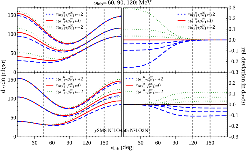
Figure 8: (Colour on-line) Sensitivity of the cross section to varying the scalar-isoscalar polarisabilities around their central values (solid line) of eq. (1.1) by $+2$ (blue dashed) and $-2$ (green dotted) units, at N³LO [$\mathcal{O}(e^{2}\delta^{3})$] using the “mean” potential $\chi$SMSN⁴LO+$450\mathrm{MeV}$+N²LO3NI; see text for details. Left: Impact on the differential cross section. Right: Relative deviation from the central value at $60$, $90$ and $120\;\mathrm{MeV}$ (innermost to outermost in each panel). At all energies, sensitivities to isovector or spin polarisabilities are practically absent. While other potentials change the overall size of the cross section by $\pm 10\%$ (see fig. 7), relative sensitivities to scalar-isoscalar polarisabilities remain near-identical. Vertical dashed lines denote the angles $\theta_{\mathrm{lab}}=\{45^{\circ};120^{\circ};150^{\circ}\}$ of figs. 6 and 7.

As in previous studies [50, 51, 60, 25], we choose a variation of the scalar-isoscalar polarisabilities by $\pm 2$ canonical units in fig. 8. This is roughly at the level of the combined statistical, theoretical and Baldin Sum Rule induced uncertainties of the scalar polarisabilities. As ⁴He is a scalar-isoscalar target, this corresponds to varying the corresponding neutron polarisability by $\pm 4$. While this is twice the variation we had considered for ³He [25], it aligns with the different linear combinations of proton and neutron polarisabilities accessible in these isotopes. Other variations are very well-determined by linear extrapolation from our results, since quadratic contributions of the polarisability variations $\delta(\alpha_{E1}^{(\mathrm{s})},\beta_{M1}^{(\mathrm{s})})$ are suppressed in the squared amplitudes.

In addition, we checked that spin and isovector-scalar polarisabilities leave no signal in ⁴He Compton observables, as expected for a perfect scalar-isoscalar target. It is worth reiterating that an extraction from deuteron and ³He data is potentially contaminated by uncertainties in the spin-isoscalar polarisabilities, most notably in $\gamma_{E1E1}^{(\mathrm{s})}$, while extractions on ⁴He will not suffer from such issues.

Since the cross section is only sensitive to $\alpha_{E1}^{(\mathrm{s})}+\beta_{M1}^{(\mathrm{s})}$ at forward angles, there one can check there consistency of data with the Baldin Sum Rule value of $14.5\pm 0.4$ [6, 7]. More interesting is the combination $\alpha_{E1}^{(\mathrm{s})}-\beta_{M1}^{(\mathrm{s})}$ which is at present much less accurately determined as $7.8\pm 1.2(\mathrm{stat})\pm 0.8(\mathrm{th})$ from the world deuteron data [2, 3, 4]; cf. eq. (1.1). Note that the combined error of $\pm 1.5$ is of the order of the $\pm 2$ variations considered here.

Figure 8 illustrates again the familiar trade-off: With increasing energy, the cross section (and hence the event rate) decreases but the sensitivity to the polarisabilities increases. The difference induced by varying the scalar-isoscalar polarisabilities at $\omega_{\mathrm{lab}}=60\;\mathrm{MeV}$ by $\pm 2$ canonical units is $\pm 3\%$ and so just as much as the thickness of the line, amounting to at best $\pm 4\;\mathrm{nb/sr}$ at the most extreme angles. At $120\;\mathrm{MeV}$, however, a variation of the crucial parameter $\alpha_{E1}^{(\mathrm{s})}-\beta_{M1}^{(\mathrm{s})}$ by $\pm 2$ changed the cross section by a near-constant $\pm 11\%$ between $\theta_{\mathrm{lab}}\approx 100^{\circ}$ and $180^{\circ}$. That translates, for example, to about $\pm 9\;\mathrm{nb/sr}$ at a realistically accessible back-angle of $150^{\circ}$. Since the forward cross section is about half of the back-angle one, the relative sensitivity to $\alpha_{E1}^{(\mathrm{s})}+\beta_{M1}^{(\mathrm{s})}$ is about twice that of $\alpha_{E1}^{(\mathrm{s})}-\beta_{M1}^{(\mathrm{s})}$; the sensitivity in the rates is comparable.

It must be emphasised that both the absolute and relative sensitivities to polarisability variations are typically very little affected by the theoretical uncertainties discussed in the preceding subsection. The effect of the discrepancies between different potentials is mitigated by the fact that a large part of that relative deviation is angle-independent, whereas the sensitivities to the scalar-isoscalar polarisabilities $\alpha_{E1}^{(\mathrm{s})}\pm\beta_{M1}^{(\mathrm{s})}$ have a rather strong angular dependence. We therefore judge that our sensitivity investigations are sufficiently reliable to be useful for current planning of experiments—as we previously argued for ³He [25]. We reiterate that our goal here is an exploratory study of magnitudes and sensitivities to the nucleon polarisabilities. A polarisability extraction will of course need to address residual theoretical uncertainties with more diligence, as was already done for the proton and deuteron in refs. [2, 49, 3, 4, 5, 64, 81].

We therefore propose that data at small angles and energies should be paired with data at larger angles and energies. The former provide important checks on data consistency with the Thomson limit and with the Baldin Sum Rule, while the latter provides the best chance for high-accuracy extractions of the scalar-isoscalar polarisability combination $\alpha_{E1}^{(\mathrm{s})}-\beta_{M1}^{(\mathrm{s})}$. Given the rather straightforward sensitivity to polarisabilities in the validity range of our theory, $\omega_{\mathrm{lab}}\in[50;120]\;\mathrm{MeV}$, we are confident a more sophisticated study using Bayesian experimental design [81] will arrive at the same result.

3.5 The Beam Asymmetry

Compton beam asymmetries can be measured at some facilities, and data are available for the proton [82, 83, 84, 85, 86, 87, 88, 89, 90]. They are dominated by the single-nucleon Thomson term, which for a charged particle at $\omega=0$ predicts a shape $(\cos^{2}\theta-1)/(\cos^{2}\theta+1)$ with extremum $-1$ at $\theta_{\mathrm{lab}}=90^{\circ}$, as is well-known from Classical Electrodynamics [91]. In our findings for ⁴He, we do not address uncertainties and sensitivities at the extreme angles $\theta_{\mathrm{lab}}\leq 10^{\circ}$ and $\theta_{\mathrm{lab}}\geq 160^{\circ}$ since the asymmetry is quite small ($\leq 0.1$) there.

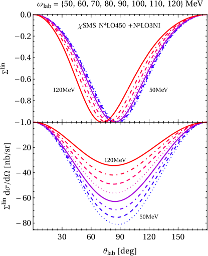
Figure 9: (Colour on-line) Evolution of the ⁴He Compton beam asymmetry (top) and its associated cross section difference (bottom) at N³LO [$\mathcal{O}(e^{2}\delta^{3})$], in the lab frame from $50$ (rightmost minimum) to $120\;\mathrm{MeV}$ (leftmost minimum) in steps of $10\;\mathrm{MeV}$, for densities generated using the “mean” potential $\chi$SMSN⁴LO+$450\mathrm{MeV}$+N²LO3NI.

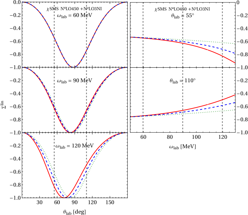
Figure 10: (Colour on-line) The beam asymmetry at N³LO [$\mathcal{O}(e^{2}\delta^{3})$] (with Delta; red solid), N²LO [$\mathcal{O}(e^{2}\delta^{2})$] (no Delta; blue dashed), and LO [$\mathcal{O}(e^{2}\delta^{0})$] (single-nucleon Thomson term only; green dotted), using the “mean” potential $\chi$SMSN⁴LO+$450\mathrm{MeV}$+N²LO3NI; see text for details. Vertical lines in the $\omega_{\mathrm{lab}}$ plots (left) correspond to the angles in the $\theta_{\mathrm{lab}}$ plots (right), and vice versa.

The top panel in fig. 9 shows the beam asymmetry itself; the bottom one half of the rate-difference, $\frac{1}{2}(\mathrm{d}\sigma^{\parallel}-\mathrm{d}\sigma^{\perp})$. While the rate-difference reduces by two-thirds from $50\;\mathrm{MeV}$ to $120\;\mathrm{MeV}$, the magnitude and shape of the (Thomson-term) asymmetry at zero energy is largely retained even between $\omega_{\mathrm{lab}}=50\;\mathrm{MeV}$ and $120\;\mathrm{MeV}$, with the extremum merely drifting towards smaller $\theta_{\mathrm{lab}}$. As an analysis of the order-by-order convergence in fig. 10 shows, this is in part a simple recoil effect of the Thomson term [LO, $\mathcal{O}(e^{2}\delta^{0})$], but the nucleons’ magnetic moments and the nucleus’ meson-exchange structure change the position of the minimum by an equal amount of about $5\%$ at the highest energies [N²LO, $\mathcal{O}(e^{2}\delta^{2})$]. Including the $\Delta(1232)$ at N³LO [$\mathcal{O}(e^{2}\delta^{3})$] shifts it yet again by about the same amount, mostly via the energy-dependent effects in $\beta_{M1}^{(\mathrm{s})}$. At $\theta_{\mathrm{lab}}=\{55^{\circ};110^{\circ}\}$, the change from N²LO to N³LO suggests an uncertainty of about $\pm 2\%$. The dependence on the $\chi$SMS $2\mathrm{N}$ and $3\mathrm{N}$ interactions in fig. 11 is quite small, namely less than thrice the thickness of the lines, and rising from a mere per-cent at $60\;\mathrm{MeV}$ to $\pm 4\%$ at $120\;\mathrm{MeV}$. Results for AV18+UIX are near-identical to $\chi$SMSN⁴LO+$550\mathrm{MeV}$+N²LO3NI; for Idaho N³LO500+3NFb, they are indistinguishable from $\chi$SMSN⁴LO+$400\mathrm{MeV}$+N²LO3NI except at $120\;\mathrm{MeV}$ where this much softer interaction adds about $+3\%$ at $30^{\circ}$ and $-2\%$ at $\gtrsim 120^{\circ}$. Following our discussion in sect. 3.3, it seems appropriate to assume a theoretical uncertainty which rises from $\pm 1\%$ at $50\;\mathrm{MeV}$ to $\pm 5\%$ at $120\;\mathrm{MeV}$. All this indicates rapid convergence in $\chi$EFT.

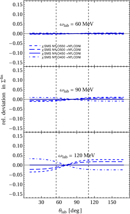
Figure 11: (Colour on-line) Energy- and angle-dependence of relative differences of the beam asymmetry for each potential, compared to the “mean” potential $\chi$SMSN⁴LO+$450\mathrm{MeV}$+N²LO3NI at N³LO [$\mathcal{O}(e^{2}\delta^{3})$]; see text for details. Vertical dashed lines denote the angles $\theta_{\mathrm{lab}}=\{55^{\circ};110^{\circ}\}$ of fig. 10. Angles $\theta_{\mathrm{lab}}\leq 10^{\circ}$ and $\theta_{\mathrm{lab}}\geq 160^{\circ}$ are not shown since they suffer from small rates and large uncertainties.

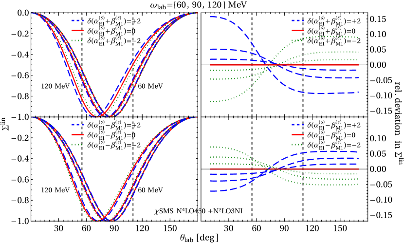
Figure 12: (Colour on-line) Sensitivity of the beam asymmetry to varying the scalar-isoscalar polarisabilities around their central values (solid line) of eq. (1.1) by $+2$ (blue dashed) and $-2$ (green dotted) units, at N³LO [$\mathcal{O}(e^{2}\delta^{3})$] using the “mean” potential $\chi$SMSN⁴LO+$450\mathrm{MeV}$+N²LO3NI; see text for details. Left: Impact on the beam asymmetry, with the minimum of $\Sigma^{\text{lin}}$ wandering to the left as $\omega_{\mathrm{lab}}$ increases. Right: Relative deviation from the central value at $60$, $90$ and $120\;\mathrm{MeV}$ (innermost to outermost in each panel). While other potentials scale the results by up to $\pm 4\%$ (see fig. 11), the relative overall sensitivities remain near-identical; see text for details. Vertical dashed lines denote the angles $\theta_{\mathrm{lab}}=\{55^{\circ};110^{\circ}\}$ of fig. 10. Relative deviations for $\theta_{\mathrm{lab}}\leq 10^{\circ}$ and $\theta_{\mathrm{lab}}\geq 160^{\circ}$ are not shown since they suffer from small rates and large uncertainties.

Given the persistence of the point-like behaviour, it should come as no surprise that the relative sensitivity to variations of the polarisabilities by $\pm 2$ units is about half of that for the cross section at the same energy; see fig. 12. Still, since measuring asymmetries is usually less prone to experimental systematic errors like beam flux and detector acceptance, high-accuracy data at moderate forward and backward angles and energies $\lesssim 120\;\mathrm{MeV}$ may provide good opportunities to extract the nucleon polarisabilities. There, sensitivities are up to $\pm 6\%$ for $\alpha_{E1}^{(\mathrm{s})}-\beta_{M1}^{(\mathrm{s})}$, and so appreciable, asymmetries are large, and cross sections (which determine rates) are still decent. Notice also that the uncertainties from the $\chi$EFT truncation and the sensitivities to the polarisability combinations $\alpha_{E1}^{(\mathrm{s})}\pm\beta_{M1}^{(\mathrm{s})}$ show different angular dependence. On the other hand, potential- and polarisability-dependence show similar angular dependence. However, the sensitivity for $\alpha_{E1}^{(\mathrm{s})}-\beta_{M1}^{(\mathrm{s})}=\pm 2$ is about twice that for the potential. Therefore, forward angles can again be used to check data consistency with the Baldin Sum Rule, and backward angles to extract $\alpha_{E1}^{(\mathrm{s})}-\beta_{M1}^{(\mathrm{s})}$ at potentially competitive levels. In that spirit, and without prejudicing thorough experimental feasibility studies, the right-hand panels of figs. 10 to 12 show the energy dependence of the beam asymmetry at two possible candidate angles, $55^{\circ}$ and $110^{\circ}$ for the three canonical choices of $\alpha_{E1}^{(\mathrm{s})}\pm\beta_{M1}^{(\mathrm{s})}$. In these cases, the variation in $\Sigma^{\rm lin}$ from varying $\alpha_{E1}^{(\mathrm{s})}-\beta_{M1}^{(\mathrm{s})}$ by $\pm 2$ translates into rate-differences of $\pm 1.6\;\mathrm{nb/sr}$.

3.6 Comparison With Other Few-Nucleon Targets

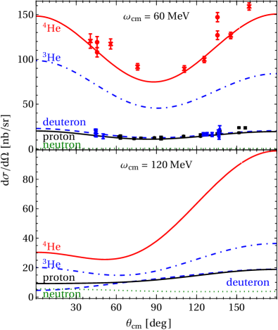
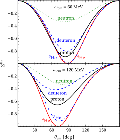
Figure 13: (Colour on-line) Comparison of the cross section (left) and beam asymmetry (right) in the centre-of-mass frame at $\omega_{\mathrm{cm}}=60\;\mathrm{MeV}$ (top) and $120\;\mathrm{MeV}$ (bottom) for a proton (black), neutron (green dotted), deuteron (blue dashed), ³He (blue dot-dashed) and ⁴He (black) target. The few-nucleon bound states use the same N³LO [$\mathcal{O}(e^{2}\delta^{3})$] kernels, including the same values for all polarisabilities, but slightly different $2\mathrm{N}$ and $3\mathrm{N}$ interactions. The cross section data at $60\;\mathrm{MeV}$ is taken on the proton (black) as discussed in [2, 49], deuteron (blue) [92], and ⁴He (blue circle: [76]; blue cross: [21]) within $\pm 5\;\mathrm{MeV}$ of the nominal energy and transformed into the centre-of-mass frame; see text for details.

To put ⁴He Compton scattering in context, we contrast the predictions with those for the proton, neutron, deuteron and ³He in fig. 13. We will not reiterate the discussion of the latter four targets in ref. [25] but focus only on their comparison to ⁴He. Each target is sensitive to different combinations of nucleon polarisabilities: the proton and neutron, by definition, only to their particular polarisabilities; the deuteron only to the isoscalar components $\alpha_{E1}^{(\mathrm{p})}+\alpha_{E1}^{(\mathrm{n})}$ etc. of both the scalar and spin polarisabilities; ³He roughly to $2\alpha_{E1}^{(\mathrm{p})}+\alpha_{E1}^{(\mathrm{n})}$, $2\beta_{M1}^{(\mathrm{p})}+\beta_{M1}^{(\mathrm{n})}$ and to the spin polarisabilities of the neutron but not of the proton; and ⁴He only to the scalar-isoscalar combinations $\alpha_{E1}^{(\mathrm{p})}+\alpha_{E1}^{(\mathrm{n})}$ and $\beta_{M1}^{(\mathrm{p})}+\beta_{M1}^{(\mathrm{n})}$ but not to any other. Each target thus provides access to complementary linear combinations.

Here, we focus on comparisons of the magnitudes of observables, important for planning experiments. At a minimum, they confirm that data on the proton, deuteron and ⁴He are consistent with our unified theory description via the complete Compton kernel at N³LO [$\mathcal{O}(e^{2}\delta^{3})$] and the same central values of eq. (1.1) for the nucleon polarisabilities. That the few-nucleon computations use slightly different $2\mathrm{N}$ and $3\mathrm{N}$ potentials, and the deuteron results include rescattering effects, is of small concern for the semi-quantitative comparison we perform here in the the régime $\omega\in[50;120]\;\mathrm{MeV}$. Likewise, there is little impact of the fact that the cross section data at $60\;\mathrm{MeV}$ have been transformed into the centre-of-mass frame but not corrected for the difference between actual and nominal experimental lab energy and angle, falling in a corridor of $\pm 5\;\mathrm{MeV}$ around the quoted energy.

In contradistinction to the other plots, the centre-of-mass (cm) frame is used in fig. 13. This avoids purely kinematic recoil effects which depend on target mass. For example, the cross section that only includes the Thomson limit [LO, $\mathcal{O}(e^{2}\delta^{0})$] is perfectly mirror-symmetric about $90^{\circ}$ in the cm frame at all energies, while its forward angles are slightly higher than back-angles in the lab frame, masking the actual amount of asymmetry caused by the target and Compton physics.

Figure 13 clearly shows that Compton cross sections on few-nucleon targets do not scale with powers of the target charge $Z$ in the region $\omega\in[50;120]\;\mathrm{MeV}$ that is of interest for extracting polarisabilities. While the proton and deuteron cross sections ($Z=1$) are of roughly similar size, the ³He and ⁴He ones are vastly different although they are both $Z=2$ targets. At $60\;\mathrm{MeV}$, the average of the ⁴He cross section over $\cos\theta_{\mathrm{cm}}$ is about twice that of ³He and nearly $7$ times of the proton and deuteron. At $120\;\mathrm{MeV}$, the ratio to ³He is nearly unchanged while that to the proton and deuteron is about $5$. At these energies, the typical photon wave length $1/\omega$ is not only comparable to the size of each nucleon constituent, but also to the range $1/m_{\pi}$ of the charged-pion exchange potential. Therefore, its effect is not “frozen out” by such a high-energy probe and the photons interact incoherently not only with each nucleon, but also with the charged long-range part of the current which glues the nucleons into a coherent, bound nucleus.

Another striking feature is how asymmetric cross sections are. One simple criterion is skewedness, which we define as the relative deviation of the cross section at $180^{\circ}$ from that at $0^{\circ}$, measured as in eq. (3.1). While at $60\;\mathrm{MeV}$, the cross section is, within $10\%$, symmetric for all targets, the situation is dramatically different at $\omega_{\mathrm{cm}}=120\;\mathrm{MeV}$: the huge skewedness of ⁴He (about $230\%$) is only matched by that of the deuteron (about $300\%$), while both ³He and the proton show only about $100\%$ relative deviation between forward and back angles. The most likely reason is that the former are isoscalar targets while the latter are $T=1/2$ ones. The rather large isovector nucleon magnetic moment substantially reduces back-scattering, countering the sizeable (isoscalar) dispersive correction from the magnetic polarisability. Angular skewedness is near-exclusively related to the one-body amplitudes; the charged-meson-exchange currents show no significant skewedness at any energy except in the much more loosely bound deuteron.

We now consider the effect of varying the neutron polarisability combination $\alpha_{E1}^{(\mathrm{n})}-\beta_{M1}^{(\mathrm{n})}$ by $\pm 2$ units, in the cm frame. For the deuteron and ⁴He this is exactly half of the variation of the scalar-isoscalar polarisability combination $\alpha_{E1}^{(\mathrm{s})}-\beta_{M1}^{(\mathrm{s})}$ by $\pm 2$ units; cf. sect. 3.4. This changes the backward-angle cross section in ⁴He at $120\;\mathrm{MeV}$ by about $\mp 5.5\%$ or $\gtrsim\pm 5\;\mathrm{nb/sr}$. The same kinematics produces a variation of about $\mp 4\%$, i.e. $\lesssim\mp 1.5\;\mathrm{nb/sr}$ in ³He and around $\gtrsim\mp 3\%$ or less than $\mp 0.6\;\mathrm{nb/sr}$ in the deuteron [50, 51, 60, 25]. So, heavier systems show both increased relative accuracy and increased rates. The absolute variation for ⁴He and ³He is qualitatively quite different because, while the polarisabilities interfere with the same Thomson term of two protons, the charged-meson-exchange part is greater in a system with more possible $\mathrm{n}\mathrm{p}$ pairs. Likewise, that for the deuteron is substantially smaller because the interference is with only one charged constituent and charged-meson-exchange between one pair only. This change in nuclear effects like binding and meson-exchange currents across different targets allows for invaluable checks that these aspects of Compton scattering dynamics are well understood.

The beam asymmetry $\Sigma^{\mathrm{lin}}$ is (except of course for the neutron) dominated by the Thomson limit of scattering on a charged point-particle at low energies. Figure 13 shows that this effect is most prominent for ⁴He and survives to higher energies than for the other targets. The extremum appears at roughly the same position for each charged target, but only in ⁴He is the minimum value of about $-1$ practically unchanged from the Thomson limit over the energy range considered. At $120\;\mathrm{MeV}$, the less-tightly bound systems only reach $-0.9$ (³He) and $-0.4$ (deuteron), and the unbound proton has $-0.65$. This may yet again demonstrate the competing effects of one-body and charged-meson-exchange contributions. The angle-dependent magnitude of the sensitivity to varying the neutron’s scalar polarisability combination $\alpha_{E1}^{(\mathrm{n})}-\beta_{M1}^{(\mathrm{n})}$ is not dissimilar in all cases, namely up to $\pm 0.02$ in magnitude or up to $\pm 3\%$ in relative deviation for ⁴He, about $3/4$ of that for ³He, and about half for the deuteron. Rate differences at $110^{\circ}$ are about $\pm 0.8\;\mathrm{nb/sr}$ in⁴He, with $\pm 0.25\;\mathrm{nb/sr}$, i.e., less than a third of that in ³He, and at $\pm 0.07\;\mathrm{nb/sr}$ in the deuteron.

A more comprehensive and rigorous discussion of target effects is left to an upcoming cross-target study of observables and their sensitivities on the polarisabilities [93].

4 Summary and Conclusions

This presentation reports the first ab initio calculation (as defined in ref. [20]) of elastic Compton scattering on ⁴He. It is carried out in $\chi$EFT at $\mathcal{O}(e^{2}\delta^{3})$ [N³LO ] in the $\delta$-expansion, as applied in the range $50\;\mathrm{MeV}\lesssim\omega_{\mathrm{lab}}\lesssim 120\;\mathrm{MeV}$. Since the scalar-isoscalar combinations of nucleon electric and magnetic polarisabilities that have already been measured in $\gamma$-deuteron scattering are exactly those that enter in this process, we take the deuteron values as input. Our calculation then has no free parameters. Compared to data from Illinois, MAXlab and HI$\gamma$S between $50$ and $80\;\mathrm{MeV}$, it predicts the correct angular dependence of the Compton differential cross section, and the right size. The energy dependence is correct within combined theory and experimental error bars, albeit the central values seem to have a different trend than the data. This overall agreement is a strong validation of $\chi$EFT’s ability to describe electromagnetic processes on light nuclei.

We predict that Compton cross sections on the deuteron [50, 51], ³He [25], and ⁴He are approximately in the ratio $1:2:5$ at $\omega=120\;\mathrm{MeV}$. This scaling is not explained by the number of constituent charges. Rather, it provides concrete evidence for the crucial rôle that pion-exchange currents, and, relatedly, $\mathrm{n}\mathrm{p}$ pairs correlated by one-pion exchange, play in determining the electromagnetic response in these nuclei for photons with energies of order $100\;\mathrm{MeV}$ [94].

Wile this study may not suffice to reliably extract polarisabilities from ⁴He data, it does suffice for reliable rate estimates and, in particular, sensitivity studies. These may be useful for planning experiments. Observables are only sensitive to the two scalar-isoscalar dipole polarisabilities of the nucleon. For the cross section, we found that the relative sensitivity to variations of the less-well-known combination $\alpha_{E1}^{(\mathrm{s})}-\beta_{M1}^{(\mathrm{s})}$ carries considerably smaller uncertainties than absolute rates. That is in part because residual theory errors are largely angle-independent, while the impact of this combination is zero at forward angles and maximal at backward angles. The dependence of the cross section on a variation by $\pm 2$ canonical units rises steadily from $\pm 3\%$ of an overall $120\;\mathrm{nb}\,\mathrm{sr}^{-1}$ at $60\;\mathrm{MeV}$ to $\pm 11\%$ of about $80\;\mathrm{nb}\,\mathrm{sr}^{-1}$ at $120\;\mathrm{MeV}$.

Therefore, we advocate for data at high energies and large angles to facilitate high-accuracy extractions of the scalar-isoscalar polarisability combination $\alpha_{E1}^{(\mathrm{s})}-\beta_{M1}^{(\mathrm{s})}$—this is also important for the deuteron and ³He. These should be complemented in the same experiment with measurements at low energies and small angles: They provide an important check of consistency with the Thomson limit and with the Baldin Sum Rule.

Measuring a ratio between forward- and back-angle cross sections may reduce theoretical uncertainties, while concurrently reducing angle-independent/systematic experimental errors. We are cautious about the usefulness of beam-asymmetry data by itself. There, theory uncertainties and polarisability sensitivities show a very similar angular dependence, and rate-differences are quite small.

We are confident in these findings, based on an assessment of the region of validity and theoretical uncertainties of our approach. In the region in which the present formalism is applicable, $50\;\mathrm{MeV}\lesssim\omega\lesssim 120\;\mathrm{MeV}$, we determined its accuracy to be about $\pm 10\%$ across energies, with possibly $\pm 12\%$ in back-scattering at the highest energies. The main theory uncertainty comes from the wave-function dependence across four $\chi$EFT potentials with different cutoffs, and is of higher order. While it is also angle-independent, we cannot use that fact to eliminate this source of theory uncertainties without additional theoretical justification. Based on experience from the deuteron case, the inclusion of the mechanisms that restore the Thomson limit should also reduce the dependence on the choice of $\chi$EFT interaction at the higher energies studied here.

This is the other respect in which the calculation should be improved, namely by including coherent propagation of the $A$-body system between interactions with the first and second Compton photon incorporated into the calculation. In the deuteron case, including these effects that restore the nuclear Thomson limit leads to a reduction of the cross section by $10\%$ to $20\%$ at $\omega=50\;\mathrm{MeV}$, but only a few percent at $120\;\mathrm{MeV}$ [50, 51]. For ⁴He, it is plausible that the corrections by coherent-nuclear effects may suppress the cross section at the low end of our energy range somewhat more: the mismatch between the Thomson-limit and the $\omega=0$ amplitude in our calculation is larger than for either the deuteron or ³He, and ⁴He has a substantially larger binding energy, so coherent propagation of the four-nucleon system is likely to be important up to higher energies than in the two- and three-nucleon case. We note that, in fact, our results already compare well with data even at $\omega\approx 50\;\mathrm{MeV}$. Work to restore the Thomson limit in few-nucleon systems is in progress [98].

Our calculation of ⁴He Compton scattering with full treatment of nuclear structure and two-body currents is tractable because we use the Transition Density Method that was developed and tested in refs. [23, 24]. As was the case for ³He and ³H, the one- and two-body densities generated for this investigation from $5$ chiral potentials as well as the AV18$+$UIX potential can be used for a cornucopia of computations of reactions involving the ⁴He system. They are available using a python package from https://pypi.org/project/nucdens/. The method also opens the way to calculations of Compton scattering on other light nuclear targets like ⁶Li.

The present investigation is part of the ongoing effort to develop a unified picture of Compton scattering on light nuclei [26, 55, 59, 27, 28, 29, 25]. The calculations carried out here use the same kernels as those of Compton scattering on ³He [25], but are one order lower than those that have been completed for the proton [49] and are in progress for the deuteron [95]. Calculations at $\mathcal{O}(e^{2}\delta^{4})$ are needed for a precision extraction of $\alpha_{E1}^{(\mathrm{s})}$ and $\beta_{M1}^{(\mathrm{s})}$ that will have theory error bars concomitant with those arising from expected future high-quality ⁴He data. Such a calculation, and its comparison with forthcoming data [96, 97], should permit a more straightforward extraction of $\alpha_{E1}^{(\mathrm{s})}-\beta_{M1}^{(\mathrm{s})}$ than was possible in deuterium, because the effect of the nucleon spin polarisabilities is very small in a scalar-isoscalar nucleus like ⁴He.

This work opens up the possibility of validating the $\chi$EFT treatment of elastic Compton scattering across a range of few-nucleon systems. Such comparisons may also aid the understanding of both systematic errors in the measurements and the rôle of charged-pion-exchange currents across few-nucleon systems: from the loosely bound deuteron via ³He to tightly bound ⁴He. The deuteron theory is well-understood and sensitive to the same linear combination of polarisabilities as ⁴He [2]. ³He computations are now available as well, probing a different combination of neutron and proton polarisabilities, $2\alpha_{E1}^{(\mathrm{p})}+\alpha_{E1}^{(\mathrm{n})}$ etc. [27, 28, 29, 25]. Deuteron, ⁴He and ⁶Li data is already available and new experiments are approved for these three targets and for ³He [97, 96]. Ultimately, a global fit across different nuclei would minimise the impact of experimental systematics in any one data set, exploit the different linear combinations of proton and neutron polarisabilities embedded in different nuclear targets, and test $\chi$EFT’s predictions for the impact of nuclear binding and charged-meson-exchange currents—all while measuring a fundamental process that characterises the strong-interaction response of the constituents of nucleons and light nuclei to electromagnetic fields.

References

- [1] C. R. Howell, M. W. Ahmed, A. Afanasev, D. Alesini, J. R. M. Annand, A. Aprahamian, D. L. Balabanski, S. V. Benson, A. Bernstein and C. R. Brune, et al. J. Phys. G 49 (2022) 010502 doi:10.1088/1361-6471/ac2827 [arXiv:2012.10843 [nucl-ex]].
- [2] H. W. Grießhammer, J. A. McGovern, D. R. Phillips and G. Feldman, Prog. Part. Nucl. Phys. 67 (2012) 841 doi:10.1016/j.ppnp.2012.04.003 [arXiv:1203.6834 [nucl-th]].
- [3] L. S. Myers et al. [COMPTON@MAX-lab Collaboration], Phys. Rev. Lett. 113 (2014) 262506 doi:10.1103/PhysRevLett.113.262506 [arXiv:1409.3705 [nucl-ex]].
- [4] L. S. Myers et al., Phys. Rev. C 92 (2015) 025203 doi:10.1103/PhysRevC.92.025203 [arXiv:1503.08094 [nucl-ex]].
- [5] H. W. Grießhammer, J. A. McGovern and D. R. Phillips, Eur. Phys. J. A 52 (2016) 139 doi:10.1140/epja/i2016-16139-5 doi:10.22323/1.253.0104 [arXiv:1511.01952 [nucl-th]].
- [6] V. Olmos de Leon et al., Eur. Phys. J. A 10 (2001) 207 doi:10.1007/s100500170132.
- [7] M. I. Levchuk and A. I. L’vov, Nucl. Phys. A 674 (2000) 449 doi:10.1016/S0375-9474(00)00145-7 [nucl-th/9909066].
- [8] O. Gryniuk, F. Hagelstein and V. Pascalutsa, Phys. Rev. D 92 (2015) 074031 doi:10.1103/PhysRevD.92.074031 [arXiv:1508.07952 [nucl-th]].
- [9] W. Detmold et al. [USQCD Collaboration], Eur. Phys. J. A 55 (2019) 193 doi:10.1140/epja/i2019-12902-4 [arXiv:1904.09512 [hep-lat]].
- [10] A. Alexandru, PoS CD 2018 (2019) 021 doi:10.22323/1.317.0021.
- [11] R. Bignell, W. Kamleh and D. Leinweber, “Magnetic polarizability of the nucleon using a Laplacian mode projection,” Phys. Rev. D 101 (2020) 094502 doi:10.1103/PhysRevD.101.094502 [arXiv:2002.07915 [hep-lat]].
- [12] W. Wilcox and F. X. Lee, Phys. Rev. D 104 (2021) 034506 doi:10.1103/PhysRevD.104.034506 [arXiv:2106.02557 [hep-lat]].
- [13] X. H. Wang, C. L. Fan, X. Feng, L. C. Jin and Z. L. Zhang, [arXiv:2310.01168 [hep-lat]].
- [14] J. Gasser, M. Hoferichter, H. Leutwyler and A. Rusetsky, Eur. Phys. J. C 75 (2015) 375 doi:10.1140/epjc/s10052-015-3580-9 [arXiv:1506.06747 [hep-ph]].
- [15] A. W. Thomas, X. G. Wang and R. D. Young, Phys. Rev. C 91 (2015) 015209 [arXiv:1406.4579 [nucl-th]].
- [16] O. Tomalak, Eur. Phys. J. Plus 135 (2020) 411 doi:10.1140/epjp/s13360-020-00413-9 [arXiv:1810.02502 [hep-ph]].
- [17] A. Walker-Loud, “On the Cottingham formula and the electromagnetic contribution to the proton-neutron mass splitting,” PoS CD 2018 (2019) 045 doi:10.22323/1.317.0045 [arXiv:1907.05459 [nucl-th]].
- [18] J. Gasser, H. Leutwyler and A. Rusetsky, “On the mass difference between proton and neutron,” Phys. Lett. B 814 (2021) 136087 doi:10.1016/j.physletb.2021.136087 [arXiv:2003.13612 [hep-ph]].
- [19] E. Mornacchi, S. Rodini, B. Pasquini and P. Pedroni, Phys. Rev. Lett. 129 (2022) 102501 doi:10.1103/PhysRevLett.129.102501 [arXiv:2204.13491 [hep-ph]].
- [20] A. Ekström, C. Forssén, G. Hagen, G. R. Jansen, W. Jiang and T. Papenbrock, Front. Phys. 11 (2023), 1129094 doi:10.3389/fphy.2023.1129094 [arXiv:2212.11064 [nucl-th]].
- [21] M. H. Sikora, M. W. Ahmed, A. Banu, C. Bartram, B. Crowe, E. J. Downie, G. Feldman, H. Gao, H. W. Grießhammer and H. Hao, et al. Phys. Rev. C 96 (2017) 055209 doi:10.1103/PhysRevC.96.055209
- [22] M. H. Sikora, private communication (2020).
- [23] H. W. Grießhammer, J. A. McGovern, A. Nogga and D. R. Phillips: Few-Body Syst. 61 (2020) 48 doi:10.1007/s00601-020-01578-w [arXiv:2005.12207 [nucl-th]].
- [24] J. de Vries, C. Köber, A. Nogga and S. Shain, [arXiv:2310.11343 [hep-ph]].
- [25] A. Margaryan, B. Strandberg, H. W. Grießhammer, J. A. Mcgovern, D. R. Phillips and D. Shukla, Eur. Phys. J. A 54 (2018) 125 doi:10.1140/epja/i2018-12554-x [arXiv:1804.00956 [nucl-th]].
- [26] S. R. Beane, M. Malheiro, D. R. Phillips and U. van Kolck, Nucl. Phys. A 656 (1999) 367 doi:10.1016/S0375-9474(99)00312-7 [nucl-th/9905023].
- [27] D. Choudhury, A. Nogga and D. R. Phillips, Phys. Rev. Lett. 98 (2007) 232303 doi:10.1103/PhysRevLett.98.232303 [nucl-th/0701078].
- [28] D. Shukla, A. Nogga and D. R. Phillips, Nucl. Phys. A 819 (2009) 98 doi:10.1016/j.nuclphysa.2009.01.003 [arXiv:0812.0138 [nucl-th]].
- [29] D. Choudhury, PhD thesis, Ohio University (2006) http://rave.ohiolink.edu/etdc/view?acc_num=ohiou1163711618.
- [30] H. W. Grießhammer, J. Liao, J. A. McGovern, A. Nogga and D. R. Phillips, Proceedings of the 16th International Conference on Meson-Nucleon Physics and the Structure of the Nucleon (MENU 2023), submitted [arXiv:2401.15673 [nucl-th]].
- [31] A. Long, H. W. Grießhammer and A. Nogga, in progress.
- [32] D. Choudhury, A. Nogga and D. R. Phillips, Phys. Rev. Lett. 98 (2007) 232303 Erratum: [Phys. Rev. Lett. 120 (2018) 249901] doi:10.1103/PhysRevLett.120.249901, doi:10.1103/PhysRevLett.98.232303 [arXiv:1804.01206 [nucl-th]], [nucl-th/0701078]].
- [33] S. Weinberg, Phys. Lett. B 251 (1990) 288 doi:10.1016/0370-2693(90)90938-3.
- [34] S. Weinberg, Nucl. Phys. B 363 (1991) 3 doi:10.1016/0550-3213(91)90231-L.
- [35] S. Weinberg, Phys. Lett. B 295 (1992) 114 doi:10.1016/0370-2693(92)90099-P [arXiv:hep-ph/9209257 [hep-ph]].
- [36] U. van Kolck, PhD thesis, University of Texas at Austin (1993).
- [37] U. van Kolck, Phys. Rev. C 49 (1994) 2932 doi:10.1103/PhysRevC.49.2932.
- [38] J. L. Friar, Few Body Syst. 22 (1997) 161 doi:10.1007/s006010050059 [nucl-th/9607020].
- [39] E. Epelbaum, H.-W. Hammer and U. G. Meißner, Rev. Mod. Phys. 81 (2009) 1773 doi:10.1103/RevModPhys.81.1773 [arXiv:0811.1338 [nucl-th]].
- [40] D. R. Phillips, Ann. Rev. Nucl. Part. Sci. 66 (2016) 421 doi:10.1146/annurev-nucl-102014-022321.
- [41] R. Machleidt and F. Sammarruca, Phys. Scripta 91 (2016) 083007 doi:10.1088/0031-8949/91/8/083007 [arXiv:1608.05978 [nucl-th]].
- [42] H.-W. Hammer, S. König and U. van Kolck, Rev. Mod. Phys. 92 (2020) 025004 doi:10.1103/RevModPhys.92.025004 [arXiv:1906.12122 [nucl-th]].
- [43] E. Epelbaum, H. Krebs and P. Reinert, Front. in Phys. 8 (2020) 98 doi:10.3389/fphy.2020.00098 [arXiv:1911.11875 [nucl-th]].
- [44] A. R. Edmonds, “Angular Momentum in Quantum Mechanics”, Princeton University Press (1974).
- [45] R. L. Workman et al. [Particle Data Group], PTEP 2022 (2022) 083C01 doi:10.1093/ptep/ptac097 and http://pdg.lbl.gov.
- [46] W. N. Polyzou, Phys. Rev. C 58 (1998), 91-95 doi:10.1103/PhysRevC.58.91 [arXiv:nucl-th/9711046 [nucl-th]].
- [47] S. N. More, S. K. Bogner and R. J. Furnstahl, Phys. Rev. C 96 (2017) 054004 doi:10.1103/PhysRevC.96.054004 [arXiv:1708.03315 [nucl-th]].
- [48] A. J. Tropiano, S. K. Bogner and R. J. Furnstahl, Phys. Rev. C 104 (2021) 034311 doi:10.1103/PhysRevC.104.034311 [arXiv:2105.13936 [nucl-th]].
- [49] J. A. McGovern, D. R. Phillips and H. W. Grießhammer, Eur. Phys. J. A 49 (2013) 12 doi:10.1140/epja/i2013-13012-1 [arXiv:1210.4104 [nucl-th]].
- [50] R. P. Hildebrandt, PhD thesis, Technische Universität München (2005) [nucl-th/0512064].
- [51] R. P. Hildebrandt, H. W. Grießhammer and T. R. Hemmert, Eur. Phys. J. A 46 (2010) 111 doi:10.1140/epja/i2010-11024-y [nucl-th/0512063].
- [52] R. J. Furnstahl, D. R. Phillips and S. Wesolowski, J. Phys. G 42 (2015) no.3, 034028 doi:10.1088/0954-3899/42/3/034028 [arXiv:1407.0657 [nucl-th]].
- [53] H. W. Grießhammer, Few Body Syst. 63 (2022) 44 doi:10.1007/s00601-022-01739-z [arXiv:2111.00930 [nucl-th]].
- [54] V. Pascalutsa and D. R. Phillips, Phys. Rev. C 67 (2003) 055202 [arXiv:nucl-th/0212024].
- [55] S. R. Beane, M. Malheiro, J. A. McGovern, D. R. Phillips and U. van Kolck, Nucl. Phys. A 747 (2005) 311 doi:10.1016/j.nuclphysa.2004.09.068 [arXiv:nucl-th/0403088].
- [56] V. Bernard, N. Kaiser, U. G. Meißner, Phys. Rev. Lett. 67 (1991) 1515 doi:10.1103/PhysRevLett.67.1515.
- [57] V. Bernard, N. Kaiser and U. G. Meißner, Int. J. Mod. Phys. E 4 (1995) 193 doi:10.1142/S0218301395000092 [arXiv:hep-ph/9501384].
- [58] R. P. Hildebrandt, H. W. Grießhammer, T. R. Hemmert and B. Pasquini, Eur. Phys. J. A 20 (2004) 293 doi:10.1140/epja/i2003-10144-9 [arXiv:nucl-th/0307070].
- [59] R. P. Hildebrandt, H. W. Grießhammer, T. R. Hemmert and D. R. Phillips, Nucl. Phys. A 748 (2005) 573 doi:10.1016/j.nuclphysa.2004.11.017 [nucl-th/0405077].
- [60] H. W. Grießhammer, Eur. Phys. J. A 49 (2013) 100 [erratum: Eur. Phys. J. A 53 (2017) 113; erratum: Eur. Phys. J. A 54 (2018) 57] doi:10.1140/epja/i2013-13100-2, doi:10.1140/epja/i2017-12311-9, doi:10.1140/epja/i2018-12502-x [arXiv:1304.6594 [nucl-th]].
- [61] M. N. Butler and M. J. Savage, Phys. Lett. B 294 (1992) 369 doi:10.1016/0370-2693(92)91535-H [hep-ph/9209204].
- [62] T. R. Hemmert, B. R. Holstein and J. Kambor, Phys. Rev. D 55 (1997) 5598 doi:10.1103/PhysRevD.55.5598 [hep-ph/9612374].
- [63] T. R. Hemmert, B. R. Holstein, J. Kambor and G. Knochlein, Phys. Rev. D 57 (1998) 5746 doi:10.1103/PhysRevD.57.5746 [nucl-th/9709063].
- [64] H. W. Grießhammer, J. A. McGovern and D. R. Phillips, Eur. Phys. J. A 54 (2018) 37 doi:10.1140/epja/i2018-12467-8 [arXiv:1711.11546 [nucl-th]].
- [65] P. Reinert, H. Krebs and E. Epelbaum, Eur. Phys. J. A 54 (2018) 86 doi:10.1140/epja/i2018-12516-4 [arXiv:1711.08821 [nucl-th]].
- [66] P. Maris, E. Epelbaum, R. J. Furnstahl, J. Golak, K. Hebeler, T. Hüther, H. Kamada, H. Krebs, U. G. Meißner, J. A. Melendez, et al. Phys. Rev. C 103 (2021) 054001 doi:10.1103/PhysRevC.103.054001 [arXiv:2012.12396 [nucl-th]].
- [67] H. Le, J. Haidenbauer, U. G. Meißner and A. Nogga, Eur. Phys. J. A 60 (2024) 3 doi:10.1140/epja/s10050-023-01219-w [arXiv:2308.01756 [nucl-th]].
- [68] D. R. Phillips, PoS CD 12 (2013) 013 doi:10.22323/1.172.0013 [arXiv:1302.5959 [nucl-th]].
- [69] U. van Kolck, Front. in Phys. 8 (2020) 79 doi:10.3389/fphy.2020.00079 [arXiv:2003.06721 [nucl-th]].
- [70] I. Tews, Z. Davoudi, A. Ekström, J. D. Holt, K. Becker, R. Briceño, D. J. Dean, W. Detmold, C. Drischler and T. Duguet, et al. Few Body Syst. 63 (2022) 67 doi:10.1007/s00601-022-01749-x [arXiv:2202.01105 [nucl-th]].
- [71] R. B. Wiringa, V. G. J. Stoks and R. Schiavilla, Phys. Rev. C 51 (1995) 38 doi:10.1103/PhysRevC.51.38 [nucl-th/9408016].
- [72] B. S. Pudliner, V. R. Pandharipande, J. Carlson and R. B. Wiringa, Phys. Rev. Lett. 74 (1995) 4396 doi:10.1103/PhysRevLett.74.4396 [nucl-th/9502031].
- [73] B. S. Pudliner, V. R. Pandharipande, J. Carlson, S. C. Pieper and R. B. Wiringa, Phys. Rev. C 56 (1997) 1720 doi:10.1103/PhysRevC.56.1720 [nucl-th/9705009].
- [74] D. R. Entem and R. Machleidt, Phys. Rev. C 68 (2003) 041001 doi:10.1103/PhysRevC.68.041001 [nucl-th/0304018].
- [75] A. Nogga, P. Navratil, B. R. Barrett and J. P. Vary, Phys. Rev. C 73 (2006) 064002 doi:10.1103/PhysRevC.73.064002 [nucl-th/0511082].
- [76] D. P. Wells, PhD thesis, University of Illinois at Urbana-Champaign (1990).
- [77] K. Fuhrberg et al., Nucl. Phys. A 591 (1995) 1 doi:10.1016/0375-9474(95)00177-3.
- [78] X. Li et al., Phys. Rev. C 101 (2020) 034618 doi:10.1103/PhysRevC.101.034618 [arXiv:1912.06915 [nucl-ex]].
- [79] R. J. Furnstahl, N. Klco, D. R. Phillips and S. Wesolowski, Phys. Rev. C 92 (2015) 024005 doi:10.1103/PhysRevC.92.024005 [arXiv:1506.01343 [nucl-th]].
- [80] J. A. Melendez, R. J. Furnstahl, D. R. Phillips, M. T. Pratola and S. Wesolowski, Phys. Rev. C 100 (2019) 044001 doi:10.1103/PhysRevC.100.044001 [arXiv:1904.10581 [nucl-th]].
- [81] J. A. Melendez, R. J. Furnstahl, H. W. Grießhammer, J. A. McGovern, D. R. Phillips and M. T. Pratola, Eur. Phys. J. A 57 (2021) 81 doi:10.1140/epja/s10050-021-00382-2 [arXiv:2004.11307 [nucl-th]].
- [82] G. Blanpied et al. [LEGS collaboration], Phys. Rev. Lett. 76 (1996) 1023 doi:10.1103/PhysRevLett.76.1023.
- [83] G. Blanpied et al. [LEGS collaboration], Phys. Rev. C64 (2001) 025203 doi:10.1103/PhysRevC.64.025203.
- [84] P. P. Martel, PhD thesis, University of Massachusetts Amherst (2013) doi:doi.org/10.7275/j1yn-de26.
- [85] V. Sokhoyan et al. [A2 Collaboration], Eur. Phys. J. A 53 (2017) 14 doi:10.1140/epja/i2017-12203-0 [arXiv:1611.03769 [nucl-ex]].
- [86] C. Collicott, PhD thesis, Dalhousie University (2015) https://wwwa2.kph.uni-mainz.de/images/publications/phd/thesis_Collicott-Cristina-2015.pdf .
- [87] P. Martel et al. [A2 Collaboration], EPJ Web Conf. 142 (2017) 01021 doi:10.1051/epjconf/201714201021.
- [88] X. Li, et al., Phys. Rev. Lett. 128 (2022) 132502 doi:10.1103/PhysRevLett.128.132502 [arXiv:2205.10533 [nucl-ex]].
- [89] D. Paudyal et al. [A2], Phys. Rev. C 102 (2020) no.3, 035205 doi:10.1103/PhysRevC.102.035205 [arXiv:1909.02032 [nucl-ex]].
- [90] E. Mornacchi et al. [A2 Collaboration at MAMI], Phys. Rev. Lett. 128 (2022) no.13, 132503 doi:10.1103/PhysRevLett.128.132503 [arXiv:2110.15691 [nucl-ex]].
- [91] J.D. Jackson, Classical Electrodynamics, Wiley, 1998.
- [92] M. Lundin, J. O. Adler, M. Boland, K. Fissum, T. Glebe, K. Hansen, L. Isaksson, O. Kaltschmidt, M. Karlsson and K. Kossert, et al. Phys. Rev. Lett. 90 (2003) 192501 doi:10.1103/PhysRevLett.90.192501 [arXiv:nucl-ex/0204014 [nucl-ex]].
- [93] H. W. Grießhammer, J. A. McGovern, A. Nogga and D. R. Phillips, in preparation.
- [94] S. Pastore, J. Carlson, S. Gandolfi, R. Schiavilla and R. B. Wiringa, Phys. Rev. C 101 (2020) 044612 doi:10.1103/PhysRevC.101.044612 [arXiv:1909.06400 [nucl-th]].
- [95] H. W. Grießhammer, J. A. McGovern and D. R. Phillips, in preparation.
- [96] D. Hornidge, Proceedings of the 16th International Conference on Meson-Nucleon Physics and the Structure of the Nucleon (MENU 2023), submitted.
- [97] G. Feldman, Proceedings of the 16th International Conference on Meson-Nucleon Physics and the Structure of the Nucleon (MENU 2023), submitted.
- [98] N. R. Walet, J. Singh, J. Kirscher, M. C. Birse, H. W. Grießhammer and J. A. McGovern, Few-Body Syst. 64 (2023) 56 doi:10.1007/s00601-023-01824-x [arXiv:2303.09361 [nucl-th]].