Zero-shot Classification using Hyperdimensional Computing

Abstract

Classification based on Zero-shot Learning (ZSL) is the ability of a model to classify inputs into novel classes on which the model has not previously seen any training examples. Providing an auxiliary descriptor in the form of a set of attributes describing the new classes involved in the ZSL-based classification is one of the favored approaches to solving this challenging task. In this work, inspired by Hyperdimensional Computing (HDC), we propose the use of stationary binary codebooks of symbol-like distributed representations inside an attribute encoder to compactly represent a computationally simple end-to-end trainable model, which we name Hyperdimensional Computing Zero-shot Classifier (HDC-ZSC). It consists of a trainable image encoder, an attribute encoder based on HDC, and a similarity kernel. We show that HDC-ZSC can be used to first perform zero-shot attribute extraction tasks and, can later be repurposed for Zero-shot Classification tasks with minimal architectural changes and minimal model retraining. HDC-ZSC achieves Pareto optimal results with a 63.8% top-1 classification accuracy on the CUB-200 dataset by having only 26.6 million trainable parameters. Compared to two other state-of-the-art non-generative approaches, HDC-ZSC achieves 4.3% and 9.9% better accuracy, while they require more than 1.85$\times$ and 1.72$\times$ parameters compared to HDC-ZSC, respectively.

I Introduction

Object recognition using classical machine learning approaches heavily depends on the availability of a sufficiently large labeled training dataset. Particularly for fine-grained classification tasks, creating high-quality annotations is expensive and time-consuming; therefore, models with generalization capability to classify images from unseen (or partially seen) classes have been studied over the past few years. Few-shot Learning has recently emerged as a popular topic of research in this regard, which attempts to rapidly train the existing models by admitting only one or very few instances of training data per class [1, 2, 3].

In an extreme case, Zero-shot Learning (ZSL) aims at classifying an object without having seen any instances from the same class during training [4, 5, 6, 7, 8, 9, 10]. To enable the recognition of previously unseen classes, in ZSL, the learner is provided with a unique descriptor that distinguishes the unseen class with respect to the classes the learner was trained on. The descriptor is typically a collection of attributes, each of which can take a finite range of values. Attributes generated per instance can be human-annotated or the captions accompanying the images [11]. A class-level descriptor can be generated by observing a sample statistic from all instance-level attribute value distributions of the class concerned. The goal of ZSL is, having seen certain combinations of values for the set of attributes, to successfully interpolate to other value combinations corresponding to the unseen classes and thereby inferring the classes of the input examples provided.

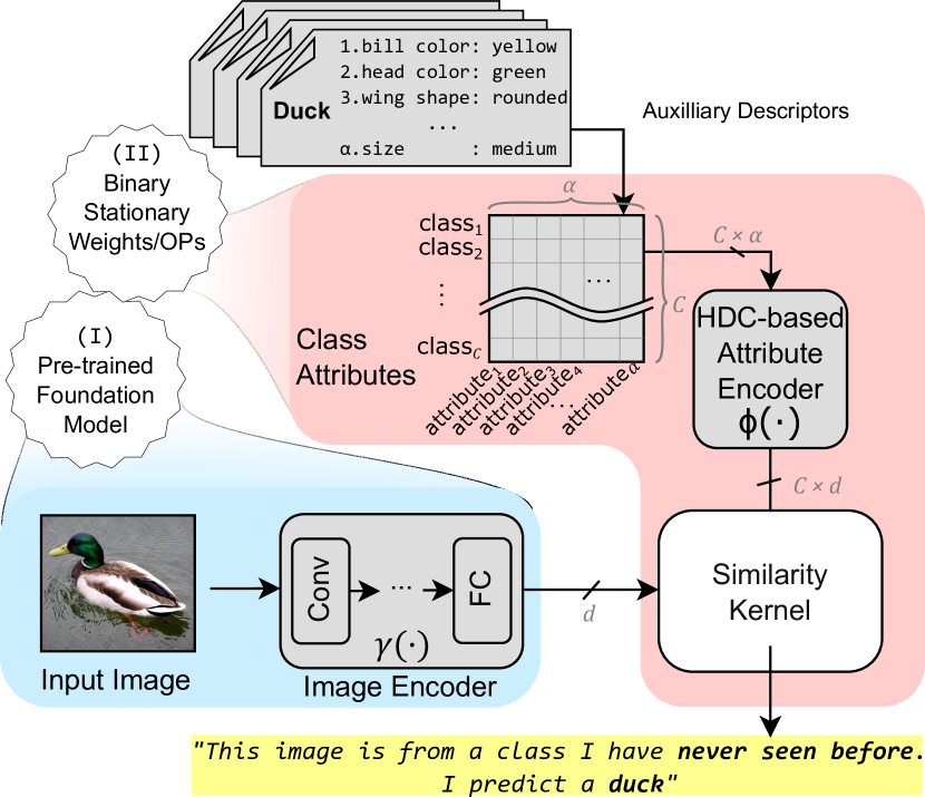
Figure 1: The general model structure employed for Zero-shot Classification in this work. It comprises two main modules: a pre-trained foundation model image encoder and an HDC-based attribute encoder. The attribute encoder consists of weights with fixed binary vectors and binary vector operations, providing opportunities for implementation in resource-constrained edge devices. Modules filled with gray color remain stationary during inference.

A ZSC model generally consists of an image encoder and an attribute encoder as shown in Fig. 1. At inference time, the image encoder accepts an image from an unseen class on which the model was not trained. In this example, a duck image is presented to the model, but no images from the duck class were provided during training. Therefore it happens to be an input from a class that the model has neither seen nor tuned to before. However, the model gets access to auxiliary information of all classes including the unseen ones via the attribute encoder. In this example, the attributes unique to the class of duck such as bill color, head color, wing shape, size, etc. are fed in as an auxiliary descriptor for the duck class. Having seen the attributes in different combinations for other classes during training, a ZSL model infers that the attributes present in the given image belong to the description of the duck class.

There are several approaches for solving ZSL problems, which can be broadly divided into two categories: non-generative and generative. In non-generative approaches, mapping functions are explored for image and attribute descriptions such that their alignments can be generalized by applying batch-level contrastive loss functions [11, 4]. The generative approaches on the other hand rely on larger models capable of artificially manufacturing instances for a given unseen class descriptor thereby helping effectively turn the problem into a few-shot learning problem [12].

This work presents a new non-generative end-to-end training method for Zero-shot Classification (ZSC) featuring attribute encoders containing fixed and compact dictionaries. Thanks to the theory of Hyperdimensional Computing (HDC) [13], these compact codebooks, representing values and attribute groups, can be initialized randomly with binary codevectors when sufficiently high dimensionality is given. HDC has recently been combined with neural networks which not only achieved the state-of-the-art accuracy in image-based few-shot learning [14] and few-shot continual learning [15, 16] but also led to energy-efficient hardware implementations. Here, we further expand this combination to the ZSC tasks.

The contributions of this work are listed below:

• Introducing a novel hybrid architecture for ZSC named HDC-ZSC. It comprises a trainable foundation model image encoder that extracts features/embeddings from images, an HDC-based fixed (stationary) attribute encoder that transforms auxiliary attributes into high-dimensional binary/bipolar vector embeddings, and finally, a kernel that measures the similarity between the two embeddings, as shown in Fig. 1.

• Proposing a training methodology to boost ZSC accuracy beyond previous state-of-the-art non-generative methods. It consists of pre-training the model on a standard image classification task at first, followed by a domain-specific attribute extraction task. Here we predict the attributes present in an image to match the ground-truth attributes of the target. In the final phase of training, the matured model is exposed to the ZSC task by retraining to discriminate attribute vectors representing the classes.

• Evaluating our model on the CUB-200 dataset on the attribute extraction task first, followed by the ZSC. For ZSC, the final HDC-ZSC achieves an average top-1 classification accuracy of 63.8% on the CUB-200 dataset. Compared to two other non-generative state-of-the-art approaches [4, 17], this is a 4.3% and 9.9% improvement in accuracy, yet our model is made up of 1.85$\times$ and 1.72$\times$ fewer parameters compared to the same reference models, respectively.

To put these results into perspective, more computationally intensive prominent generative approaches require 1.75$\times$–2.58$\times$ more parameters while their accuracies reach only a meager 3.9% increase compared to HDC-ZSC. When compared with both state-of-the-art generative and non-generative approaches, HDC-ZSC, and its variants, are in the Pareto front with respect to accuracy and model parameter count (see Fig. 4). This could potentially pave the way for its implementation as an application target in low-power embedded platforms [18].

II Background

Zero-shot Learning

The human brain is able to learn new concepts by encountering a few examples or applying deductive, inductive, or abductive reasoning. However, the training of classical machine learning models, deep learning models, in particular, rely on a large dataset with an adequate number of training examples for each class. The idea of ZSL stems from the quest for general artificial intelligence models capable of recognizing classes having seen zero or a few instances thereof similar to the way the brain functions. In fact, some argue that one-shot learning is a specific case of ZSL called transductive ZSL, in which the attribute descriptors are provided in an unstructured pictorial form [19]. In ZSL the learner is first exposed to a training dataset $\mathcal{D}_{r}$ composing of: (i) the input object set $\mathcal{X}_{r}=\{\mathbf{x}_{1_{r}},\mathbf{x}_{2_{r}},...,\mathbf{x}_{N_{r}}\}$ which are three-dimensional matrices in the case of images, and $N_{r}$ stands for the number of training samples, (ii) the set of class labels $\mathcal{Y}_{r}$ associated with the input objects, (iii) the class attribute matrix $\mathbf{A}_{r}\in\mathbb{R}^{C_{r}\,\times\,\alpha}$, which consists of an attribute vector of length $\alpha$, per unique class. $C_{r}$ represents the total number of unique classes in the training dataset and, $\alpha$ refers to the number of attributes that are identifiable across training and testing datasets.

Similarly, a testing dataset $\mathcal{D}_{e}$ can be defined with $\mathcal{X}_{e}$, $N_{e}$, $\mathcal{Y}_{e}$, $\mathbf{A}_{e}$, $C_{e}$ referring to the testing dataset’s input object set, number of samples, class label set, class attribute matrix, and the number of unique classes, respectively. In ZSL, the set of class labels in the training and testing datasets are mutually exclusive ($\mathcal{Y}_{r}\bigcap\mathcal{Y}_{e}=\emptyset$).

All ZSL methods associate seen and unseen classes through some form of auxiliary descriptors which encodes distinguishing properties of objects (e.g., language description, attributes, etc.), and establish links between previously seen data and new unseen data. Different ZSL methods have been developed in the past years. The notable types include (i) Learning Linear Compatibility [20], [4], [7], in which a linear connection is learned between image and attribute encodings, (ii) Learning Non-Linear Compatibility [21], [22], in which the learned connection is non-linear, (iii) Learning Intermediate Attribute Classifiers [23], in which an attribute predictor’s scores are used for class prediction, (iv) Hybrid Models [6], [8], [24], [25], which measures semantic similarity between images and attributes. Additionally, there exist approaches based on Generative Adversarial Network [26], [12], [27], [28], which employ supplementary networks to generate unseen class examples during training.

This work follows the linear compatibility approach similar to ESZSL [4] and CLIP [11]. ESZSL uses the squared loss to learn the bilinear compatibility and regularizes the objective w.r.t Frobenius norm, whereas CLIP tries to maximize the cosine similarity of correct image-attribute pairs while minimizing the same for incorrect pairs.

Hyperdimensional Computing (HDC)

HDC is a vector space model that encodes symbols starting from randomly initialized high-dimensional vectors called atomic hypervectors. It has been shown that as the dimensionality of the vector space grows, randomly initialized vectors tend to become quasi-orthogonal to each other [13]. As one use-case of HDC, the quasi-orthogonal atomic hypervectors representing a key vector can be combined with the corresponding value vector using a variable binding operation ($\odot$) to generate a hypervector that represents the compound symbol within the same dimensional space. In addition to the binding operation, HDC is defined by several other elementary algebraic operations such as bundling ($+$), permutation ($\rho$), and unbinding ($\oslash$). Hardware prototype of HDC showed substantial energy savings and extremely robust operation [29].

III Methods

In this work, an end-to-end approach for ZSL is proposed, exploiting class-attribute association and HDC. The concept is illustrated in Fig. 1. The inputs to the model are provided in two modalities: (i) a batch of images $\mathbf{X}=(\mathbf{x}_{1},\mathbf{x}_{2},...,\mathbf{x}_{B})$ in matrix form with batch size $B$, and (ii) a class attributes matrix $\mathbf{A}=(\mathbf{a}_{1},...,\mathbf{a}_{C})\in\mathbb{R}^{C\times\alpha}$, where each row is an attribute vector of $\alpha$ dimension with $C$ vectors in total representing all classes. The images of dimensions $h,w,l$ are passed through an image encoder $\gamma(\cdot):\mathbb{R}^{h\times w\times l}\rightarrow\mathbb{R}^{d}$ and the attributes are passed through an attribute encoder $\phi(\cdot):\mathbb{R}^{\alpha}\rightarrow\mathbb{R}^{d}$, both of which generate embeddings of the same dimensionality ($d$). The embeddings are then compared via a bi-similarity kernel cossim, that relates image and class embeddings [4], [11], as follows:

$$cossim(\gamma(\mathbf{X}),\phi(\mathbf{A}))=\frac{1}{K}\,\frac{\gamma(\mathbf{X})^{T}\cdot\phi(\mathbf{A})}{||\gamma(\mathbf{X})||\,\,||\phi(\mathbf{A})||},$$

where $K$ is the learnable temperature scaling parameter. The resulting similarity matrix of dimension $B\times C$ is used for error computation with respect to the batch of ground-truth labels and updating the image encoder’s weights over a series of epochs. Finally, the predicted class for every unseen queried image $\mathbf{x}$ is computed as

$$\hat{\mathbf{y}}=\operatorname*{arg\,max}_{i\in\{1,...,C\}}\,cossim(\gamma(\mathbf{x}),\phi(\mathbf{a}_{i})).$$

In summary, our approach employs three main computational modules:

• Image Encoder $\gamma(\cdot)$: extracts embeddings from images;

• Attribute Encoder $\phi(\cdot)$: extract embeddings from class attributes;

• Similarity Kernel: measure the similarity (e.g., dot-product, cosine similarity) between image and attribute embeddings.

III-A HDC-based Attribute Extraction

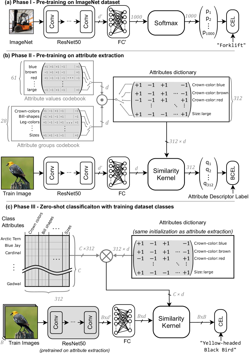
Figure 2: Different phases of Zero-shot Classification training. (a) The backbone network is pre-trained on ImageNet data (b) The backbone network and the projection FC are pre-trained on attribute extraction (c) The backbone network and the projection FC are further fine-tuned with training on Zero-shot Classification task with images of classes in the training dataset. Modules filled with gray color are stationary.

The attribute encoder first assigns randomly initialized $d$-dimensional binary/bipolar dense random hypervectors to all atomic level symbols. Dense random hypervector generation can be easily realized by sampling from the Rademacher distribution. With a sufficiently high dimension, the atomic vectors tend to be quasi-orthogonal to each other.

In this task, we identify atomic hypervectors from two codebooks. They are the attribute groups codebook ($\mathbf{g}_{1},\mathbf{g}_{2},...,\mathbf{g}_{G}$) and the attribute values codebook ($\mathbf{v}_{1},\mathbf{v}_{2},...,\mathbf{v}_{V}$). By assigning an atomic hypervector for the two sources separately instead of assigning one for each appropriate attribute group/value combination ($\mathbf{b}_{1},\mathbf{b}_{2},...,\mathbf{b}_{\alpha}$), we reduce the memory requirement For example, in the CUB-200 dataset, there are $\alpha=312$ attribute group/value combinations; however, there are only $G=28$ groups (e.g., crown colors, leg colors, sizes, etc.) and $V=61$ unique values (e.g., blue, brown, large, etc.). This leads to a 71% reduction in memory requirement for storing atomic hypervectors. This results in just 17 KB of memory for storing the atomic hypervectors which is a negligible amount compared to the image encoder memory requirement which is typically several hundreds of MB.

The next step involves binding appropriate group and value hypervectors together using variable binding to materialize the attribute level codevectors on the fly. As described in [30], for dense bipolar hypervectors, this is simply an elementwise multiplication operation (for binary hypervectors the operation becomes elementwise XOR operation) ($\odot$) as in $\mathbf{b}_{x}=\mathbf{g}_{y}\odot\mathbf{v}_{z}$. This shows how $x^{th}\in\{1,...,\alpha\}$ attribute vector $\mathbf{b}_{x}$ in the attribute dictionary is generated implicitly by binding appropriate $y^{th}\in\{1,...,G\}$ group and $z^{th}\in\{1,...,V\}$ value hypervectors from the corresponding codebooks. According to the theory of HDC, the binding operation produces vectors quasi-orthogonal to the operand vectors. Hence it allows for preserving quasi-orthogonality at the attribute level.

During the attribute prediction, the matrix containing the attribute vectors $\mathbf{B}=~{}(\mathbf{b}_{1},\mathbf{b}_{2},...,\mathbf{b}_{\alpha})\in\{-1,+1\}^{\alpha\times d}$ is fed to the similarity kernel which additionally takes the output embedding by the image encoder $\gamma(\mathbf{x})\in\mathbb{R}^{d}$ and performs cosine similarity calculation as $\mathbf{q}=cossim(\gamma(\mathbf{x}),\mathbf{B})$.

For the image encoder, we use ResNet50 as the backbone network followed by a single fully connected (FC) layer as the image encoder. As shown in Fig. 2(a) the backbone network is pre-trained with ImageNet1K data by connecting the backbone network to the 1000-dimensional softmax layer via a temporary $FC^{\prime}$ layer in phase I. Once this pre-training stage is complete the backbone network is retained with the updated weights for phase II while the $FC^{\prime}$ layer is replaced with a $FC$ layer which is used to project the backbone network embeddings to a dimension ($d$) preferred by ZSC tasks. The process is pictorially illustrated in Fig. 2(b). The image encoder after pre-training for the attribute extraction task has matured weights in both the backbone network and the $FC$ layer so that it can be used as the starting point for ZSC in phase III.

There is a large class imbalance in the attribute extraction task due to the dominating number of inactive attributes (e.g., only one color attribute per color group is typically activated at a time among all 15 possible values). For this reason, a weighted Binary Cross Entropy Loss (BCEL) is employed between the similarity vector $\mathbf{q}$ and the ground-truth attributes. The loss is used to update the weights of both the $FC$ layer and the ResNet50 using backpropagation while keeping the attribute encoder designed with codevectors fixed.

III-B Zero-shot Classification (ZSC)

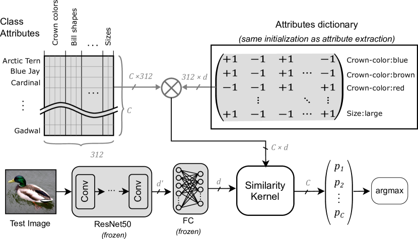
Figure 3: HDC-ZSC for Inference in Zero-shot Classification. Weights in both image and attribute encoders are stationary.

Fig. 2(c) shows the training procedure of HDC-ZSC for ZSC. The image encoder $\gamma(\cdot)$ is pre-trained on ImageNet1K data as well as on the attribute extraction task (see Section III-A). As the first step, the attribute encoder $\phi(\cdot)$ is defined as the product between the class attributes matrix $\mathbf{A}\in\mathbb{R}^{C\times\alpha}$ and the attribute vector matrix ($\mathbf{B}\in\{-1,+1\}^{\alpha\times d}$), that was populated during attribute extraction task as given in $\phi=\mathbf{A}\times\mathbf{B}$.

The result of the attribute and image encoders are fed to the similarity kernel, which computes class logits via $\mathbf{p}=cossim(\gamma(\mathbf{x}),\phi)$. Cross entropy loss (CEL) between $p$ and the ground-truth class is used to update the $FC$ layer weights in $\gamma$ over several epochs so that the image embeddings are aligned with the attribute embeddings. Having been pre-trained on ImageNet1K and attribute extraction, the backbone network remains stationary during this fine-tuned retraining step.

Finally, the trained model is deployed for ZSC inference as shown in Fig. 3. All weights of the model remain stationary at this stage.

IV Experiments

IV-A Experimental Setup

Dataset

We demonstrate the effectiveness of our framework on Caltech-UCSD Birds-200-2011 (CUB-200-2011) [31], a fine-grained dataset of 200 bird species containing 11,788 images in total. The dataset contains continuous class attributes (312-dimensional visual attributes) which are used as the class attribute matrix $\mathbf{A}$. We evaluate our model on two commonly used train-test splits, available in the literature, namely: (i) noZS where samples of 100 classes are available in each of train and test datasets, (ii) ZS where 150 classes are available for training and the remaining 50 classes for testing.

Evaluation Metrics

We use the top-1% accuracy as a metric for the attribute extraction task. To address the class imbalance issue, we use the Weighted Mean Average Precision (WMAP) as another metric. WMAP is a modified version of Average Precision designed to compensate for attributes that are less frequent in the dataset. For ZSC, a commonly used top-1 and top-5 accuracy is employed.

Implementation Details

We resize input images to 256$\times$256 and augment the training dataset with random rotation in the range of $[-45^{\circ},+45^{\circ}]$, center cropping, and random horizontal flip, before feeding them to the image encoder for both attribute and class extraction task. We implemented our framework in Pytorch and optimized it using AdamW optimizer [32] with default settings and cosine annealing learning rate scheduler [33]. Finally, the results are obtained on the aforementioned metrics by running five trials with different seeds, and average and standard deviation results are reported as: $\mu\pm\sigma$.

IV-B Experimental Results

Attribute extraction

Table I summarizes the results of weighted mean average precision (WMAP) and top-1% accuracy, comparing our approach with Finetag [34] and A3M [35] respectively. To facilitate a fair comparison, noZS split is used as was the case in the works compared against. The results show that our HDC-ZSC outperforms the previous approaches across both the metrics, by $+4.14\%$ and $+36.71\%$ respectively.

TABLE I: Attribute extraction task results comparison with Finetag and A3M using W_MAP and top-1% accuracy as evaluation metric

Attribute Group	Finetag (W_MAP)	Ours (W_MAP)	A3M (top-1% acc)	Ours (top-1% acc)
bill shape	54	58	60	90
wing color	57	60	45	90
upperpart color	55	57	43	90
underpart color	59	62	58	93
breast pattern	15	61	58	81
back color	50	53	45	91
tail shape	25	25	34	84
uppertail color	40	42	43	93
head pattern	30	33	35	89
breast color	58	61	57	92
throat color	57	61	60	93
eye color	76	76	81	98
bill length	73	76	72	80
forehead color	56	59	51	92
tail collor	42	44	38	90
nape color	55	58	49	92
belly color	58	61	59	93
wing shape	24	25	32	80
size	55	56	58	81
shape	47	49	57	94
back pattern	44	45	46	77
tail pattern	41	43	43	77
belly pattern	60	62	62	81
primary color	62	66	51	90
leg color	32	37	46	92
bill color	42	47	47	91
crown color	56	60	53	93
wing pattern	48	50	48	72
average	48.96	53.11	51.11	87.82

Zero-shot Classification

Fig. 4 compares HDC-ZSC accuracy performance and number of parameters with other state-of-the-art approaches, both generative and non-generative methods. Additionally, results from an alternative Trainable-MLP model, in which fixed HDC codebooks-based attribute encoders are replaced by 2-layer trainable MLP, are included in the table for reference. When compared to generative methods, our models reduce the number of total network parameters by more than 1.75$\times$–2.58$\times$ while maintaining a competitive top-1% accuracy. Specifically, comparing HDC-ZSC with ESZSL [4], as a non-generative model similar to our approach, we obtain a $+9.9\%$ accuracy improvement while improving the parameter efficiency by more than 1.72$\times$. As it is shown later in Section IV-C, our models train with a minimal number of epochs which enlarges computational cost savings even further compared to the above parameter savings.

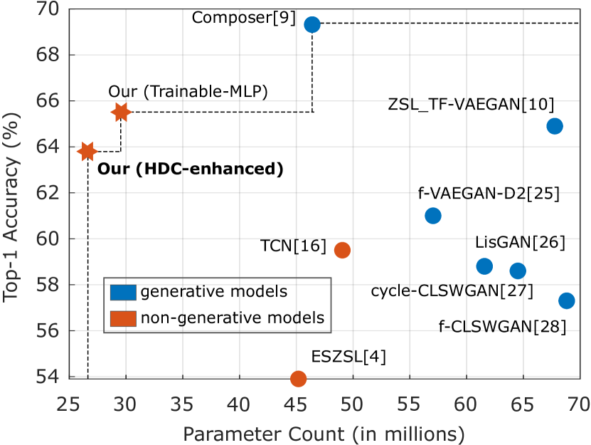
Figure 4: Comparison of Zero-shot Classification accuracy vs model parameter count. Our models HDC-ZSC and Trainable-MLP model are both in the Pareto front.

IV-C Ablation study and hyperparameter tuning

We present results from training image and attribute encoders of different complexity and maturity in Table II. This result is obtained with a common hyperparameter set without model-wise tuning. From this, we choose the best performing $ResNet50$ with an $FC$ projection layer of $d=1536$ as the preferred configuration of the image encoder for our models. Note that this preferred configuration outperforms the relatively larger $ResNet101$-based image encoder in terms of Top-1% accuracy. Further investigations could be carried out as a part of future work to find configurations that suit even more lightweight image encoders.

TABLE II: Training of different image and attribute encoders. Pre-training stage II is skipped when the projection $FC$ layer is absent. The figure of merit is Top-1% accuracy

Image Encoder	Pre-train	$d$	Attribute Encoder
			HDC ZSC	MLP Trainable
ResNet50	I,III	2048	55	60
ResNet50+FC	I,II,III	1536	58	61
	I,II,III	2048	50	57
ResNet101	I,III	2048	53	56

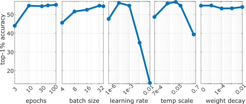
Figure 5: Hyperparameter tuning for HDC-ZSC on validation split (50 disjoint classes).

Fig. 5 provides results from the hyper-parameter exploration for HDC-ZSC. The hyperparameters explored include number of epochs, batch size, learning rate, temperature scale, and weight decay. One interesting observation is that the number of epochs required to achieve the best accuracy is around 10 which enables ZSC training to be realized in a reasonable time in low-power hardware systems. The final accuracies are reported with the best-performing hyper-parameter combination is adopted.

V Conclusions and outlook

In this work, we present the concept of integrating lightweight HDC-enhanced attribute encoders in the backend of non-generative Zero-shot Learning models. This approach allows for reducing the model parameter count by representing attributes in compact and stationary codebooks leading to over 1.72$\times$ model parameter storage efficiency while improving top-1 classification accuracy by over 4.3% compared to other non-generative approaches.

This outcome opens avenues to explore hardware implementations of the model for both inference and minimal training in low-power heterogeneous embedded systems such as the one described in [36]. For example, the convolutional image encoder can be processed in a general-purpose processor cluster, or any convolutional accelerator, whereas the stationary binary attribute encoder weights and similarity kernel operations can be offloaded to analog [37] or digital [38] non-von Neumann accelerators.

References

- [1] O. Vinyals, C. Blundell, T. Lillicrap et al., “Matching networks for one shot learning,” Advances in Neural Information Processing Systems (NeurIPS), vol. 29, 2016.
- [2] J. Snell, K. Swersky, and R. Zemel, “Prototypical networks for few-shot learning,” Advances in Neural Information Processing Systems (NeurIPS), vol. 30, 2017.
- [3] V. Sunder, A. Srinivasan, L. Vig et al., “One-shot information extraction from document images using neuro-deductive program synthesis,” International Workshop on Neural-Symbolic Learning and Reasoning (NeSy), 2019.
- [4] B. Romera-Paredes and P. Torr, “An embarrassingly simple approach to zero-shot learning,” in Proceedings of the 32nd International Conference on Machine Learning (ICML), vol. 37. PMLR, 2015, pp. 2152–2161.
- [5] E. Altszyler, P. Brusco, N. Basiou et al., “Zero-shot multi-domain dialog state tracking using descriptive rules,” International Workshop on Neural-Symbolic Learning and Reasoning (NeSy), 2020.
- [6] M. Norouzi, T. Mikolov, S. Bengio et al., “Zero-shot learning by convex combination of semantic embeddings,” arXiv preprint arXiv:1312.5650, 2013.
- [7] E. Kodirov, T. Xiang, and S. Gong, “Semantic autoencoder for zero-shot learning,” in Proceedings of the IEEE Conference on Computer Vision and Pattern Recognition (CVPR), 2017, pp. 3174–3183.
- [8] Z. Zhang and V. Saligrama, “Zero-shot learning via semantic similarity embedding,” in Proceedings of the IEEE International Conference on Computer Vision (ICCV), December 2015.
- [9] D. Huynh and E. Elhamifar, “Compositional fine-grained low-shot learning,” arXiv preprint arXiv:2105.10438, 2021.
- [10] S. Narayan, A. Gupta, F. S. Khan et al., “Latent embedding feedback and discriminative features for zero-shot classification,” in European Conference on Computer Vision (ECCV). Springer, 2020, pp. 479–495.
- [11] A. Radford, J. W. Kim, C. Hallacy et al., “Learning transferable visual models from natural language supervision,” in International Conference on Machine Learning (ICML). PMLR, 2021, pp. 8748–8763.
- [12] J. Li, M. Jing, K. Lu et al., “Leveraging the invariant side of generative zero-shot learning,” in 2019 IEEE/CVF Conference on Computer Vision and Pattern Recognition (CVPR), 2019, pp. 7394–7403.
- [13] P. Kanerva, “Hyperdimensional computing: An introduction to computing in distributed representation with high-dimensional random vectors,” Cognitive Computation, vol. 1, no. 2, pp. 139–159, 2009.
- [14] G. Karunaratne, M. Schmuck, M. Le Gallo et al., “Robust high-dimensional memory-augmented neural networks,” Nature Communications, vol. 12, no. 1, pp. 1–12, 2021.
- [15] M. Hersche, G. Karunaratne, G. Cherubini et al., “Constrained Few-shot Class-incremental Learning,” in Conference on Computer Vision and Pattern Recognition (CVPR), 2022.
- [16] G. Karunaratne, M. Hersche, J. Langeneager et al., “In-memory realization of in-situ few-shot continual learning with a dynamically evolving explicit memory,” in IEEE 48th European Solid State Circuits Conference (ESSCIRC), 2022, pp. 105–108.
- [17] H. Jiang, R. Wang, S. Shan et al., “Transferable contrastive network for generalized zero-shot learning,” CoRR, vol. abs/1908.05832, 2019.
- [18] P. D. Schiavone, D. Rossi, A. Pullini et al., “Quentin: an ultra-low-power pulpissimo soc in 22nm fdx,” in 2018 IEEE SOI-3D-Subthreshold Microelectronics Technology Unified Conference (S3S), 2018, pp. 1–3.
- [19] Y. Xian, C. H. Lampert, B. Schiele et al., “Zero-shot learning—a comprehensive evaluation of the good, the bad and the ugly,” IEEE Transactions on Pattern Analysis and Machine Intelligence, vol. 41, no. 9, pp. 2251–2265, 2018.
- [20] Z. Akata, F. Perronnin, Z. Harchaoui et al., “Label-embedding for image classification,” IEEE Transactions on Pattern Analysis and Machine Intelligence, vol. 38, no. 7, pp. 1425–1438, 2015.
- [21] Y. Xian, Z. Akata, G. Sharma et al., “Latent embeddings for zero-shot classification,” in Proceedings of the IEEE Conference on Computer Vision and Pattern Recognition (CVPR), 2016, pp. 69–77.
- [22] R. Socher, M. Ganjoo, C. D. Manning et al., “Zero-shot learning through cross-modal transfer,” Advances in Neural Information Processing Systems (NeurIPS), vol. 26, 2013.
- [23] C. H. Lampert, H. Nickisch, and S. Harmeling, “Attribute-based classification for zero-shot visual object categorization,” IEEE Transactions on Pattern Analysis and Machine Intelligence, vol. 36, pp. 453–465, 2014.
- [24] S. Changpinyo, W.-L. Chao, B. Gong et al., “Synthesized classifiers for zero-shot learning,” in Proceedings of the IEEE Conference on Computer Vision and Pattern Recognition (CVPR), 2016, pp. 5327–5336.
- [25] V. K. Verma and P. Rai, “A simple exponential family framework for zero-shot learning,” in Machine Learning and Knowledge Discovery in Databases. Springer International Publishing, 2017, pp. 792–808.
- [26] Y. Xian, S. Sharma, B. Schiele et al., “F-VAEGAN-D2: A feature generating framework for any-shot learning,” in Proceedings of the IEEE/CVF Conference on Computer Vision and Pattern Recognition (CVPR), 2019.
- [27] R. Felix, I. Reid, G. Carneiro et al., “Multi-modal cycle-consistent generalized zero-shot learning,” in Proceedings of the European conference on computer vision (ECCV), 2018, pp. 21–37.
- [28] Y. Xian, T. Lorenz, B. Schiele et al., “Feature generating networks for zero-shot learning,” in Proceedings of the IEEE Conference on Computer Vision and Pattern Recognition (CVPR), 2018, pp. 5542–5551.
- [29] A. Rahimi, P. Kanerva, and J. M. Rabaey, “A robust and energy-efficient classifier using brain-inspired hyperdimensional computing,” in Proceedings of the 2016 International Symposium on Low Power Electronics and Design (ISLPED), 2016.
- [30] M. Schmuck, L. Benini, and A. Rahimi, “Hardware optimizations of dense binary hyperdimensional computing: Rematerialization of hypervectors, binarized bundling, and combinational associative memory,” ACM Journal on Emerging Technologies in Computing Systems (JETC), vol. 15, no. 4, pp. 1–25, 2019.
- [31] C. Wah, S. Branson, P. Welinder et al., “Cub-200 2011 dataset,” California Institute of Technology, Tech. Rep. CNS-TR-2011-001, 2011.
- [32] I. Loshchilov and F. Hutter, “Decoupled weight decay regularization,” in International Conference on Learning Representations (ICLR), 2019.
- [33] ——, “SGDR: Stochastic gradient descent with warm restarts,” arXiv preprint arXiv:1608.03983, 2016.
- [34] R. Zakizadeh, M. Sasdelli, Y. Qian et al., “Finetag: Multi-attribute classification at fine-grained level in images,” arXiv preprint arXiv:1806.07124, 2018.
- [35] K. Han, J. Guo, C. Zhang et al., “Attribute-aware attention model for fine-grained representation learning,” in Proceedings of the 26th ACM international conference on Multimedia, 2018, pp. 2040–2048.
- [36] A. Garofalo, G. Ottavi, F. Conti et al., “A heterogeneous in-memory computing cluster for flexible end-to-end inference of real-world deep neural networks,” IEEE Journal on Emerging and Selected Topics in Circuits and Systems (JETCAS), vol. 12, no. 2, pp. 422–435, 2022.
- [37] R. Khaddam-Aljameh, M. Stanisavljevic, J. F. Mas et al., “Hermes-core—a 1.59-tops/mm 2 pcm on 14-nm cmos in-memory compute core using 300-ps/lsb linearized cco-based adcs,” IEEE Journal of Solid-State Circuits, vol. 57, no. 4, pp. 1027–1038, 2022.
- [38] M. Eggimann, A. Rahimi, and L. Benini, “A 5 w standard cell memory-based configurable hyperdimensional computing accelerator for always-on smart sensing,” IEEE Transactions on Circuits and Systems I: Regular Papers, vol. 68, no. 10, pp. 4116–4128, 2021.