Krasnoselskii-Mann Iterations: Inertia, Perturbations and Approximation

Abstract

This paper is concerned with the study of a family of fixed point iterations combining relaxation with different inertial (acceleration) principles. We provide a systematic, unified and insightful analysis of the hypotheses that ensure their weak, strong and linear convergence, either matching or improving previous results obtained by analysing particular cases separately. We also show that these methods are robust with respect to different kinds of perturbations–which may come from computational errors, intentional deviations, as well as regularisation or approximation schemes–under surprisingly weak assumptions. Although we mostly focus on theoretical aspects, numerical illustrations in image inpainting and electricity production markets reveal possible trends in the behaviour of these types of methods.

1 Introduction

Let $\mathcal{H}$ be a real Hilbert space. Krasnoselskii-Mann iterations Krasnoselskii ; Mann approximate fixed points of a (quasi) nonexpansive operator $T:\mathcal{H}\to\mathcal{H}$, by means of the update rule

$$x_{k+1}=(1-\lambda_{k})x_{k}+\lambda_{k}Tx_{k},$$

where $\lambda_{k}\in(0,1)$ is a relaxation parameter. They were independently introduced by Mann in 1953 Mann , with $\lambda_{k}=\frac{1}{k+1}$, and by Krasnoselskii in 1955 Krasnoselskii , with $\lambda_{k}\equiv\frac{1}{2}$. Their weak convergence was established in (Schaefer1957berDM, , Krollar 2.1) for any constant parameter $\lambda_{k}\equiv\lambda\in(0,1)$, and then in (GROETSCH1972369, , Corollary 3) for variable relaxation parameters satisfying $\sum\lambda_{k}(1-\lambda_{k})=\infty$. Krasnoselskii-Mann iterations are central to numerical optimization and variational analysis, where many problems can be reduced to finding fixed points of appropriate operators. Many known splitting optimization algorithms are special instances.

On the other hand, the consideration of physical principles has proven to be a useful technique in optimization. The concept of momentum was first introduced by Polyak in 1964 POLYAK19641 , who showed that the Heavy Ball method accelerates convergence in certain problems. Although originally proposed for gradient descent methods, it may be extended to Krasnoselskii-Mann iterations alvarez2001inertial ; AccKM ; dong2022new , giving

$$\begin{cases}y_{k}&=\quad x_{k}+\alpha_{k}(x_{k}-x_{k-1})\\ x_{k+1}&=\quad(1-\lambda_{k})y_{k}+\lambda_{k}Tx_{k},\end{cases}$$

where $\alpha_{k}$ is an acceleration parameter. The idea of momentum was later reinterpreted by Nesterov in 1983 Nesterov , also to accelerate the convergence of gradient methods. Since then, many algorithms have been improved by the addition of this more popular acceleration step, especially in the context of convex optimization beck2009fast ; doi:10.1137/0802032 , although this is not our emphasis here. Nesterov’s acceleration scheme has also been used in fixed-point theory and variational analysis boct2015inertial ; Dong ; iyiola2021new ; mainge2008convergence ; FierroMaulenPeypouquet ; MOUDAFI2003447 ; shehu2018convergence , under the form

$$\begin{cases}z_{k}&=\quad x_{k}+\beta_{k}(x_{k}-x_{k-1})\\ x_{k+1}&=\quad(1-\lambda_{k})z_{k}+\lambda_{k}Tz_{k},\end{cases}$$

where $\beta_{k}$ is an inertial parameter (observe the differences and similarities with Polyak’s approach). These two interpretations of inertia can be combined into a more general algorithm Dong2022 ; Dong2018 ; dong2021general ; gebregiorgis2023convergence

$$\begin{cases}y_{k}&=\quad x_{k}+\alpha_{k}(x_{k}-x_{k-1})\\ z_{k}&=\quad x_{k}+\beta_{k}(x_{k}-x_{k-1})\\ x_{k+1}&=\quad(1-\lambda_{k})y_{k}+\lambda_{k}Tz_{k}.\end{cases}$$

This not only provides a unified setting for the study of the classical inertial methods described above, but its versatility also suggests new ones. For instance, for $\alpha_{k}\equiv 0$, we obtain the reflected Krasnoselskii-Mann iterations Dong2022 ; Dong2018 ; doi:10.1080/10556788.2021.1924715 ; moudafi2018reflected , inspired by the reflected gradient method malitsky2015projected .

The purpose of this work is threefold:

1. First, to provide a systematic and unified analysis of the hypotheses that ensure the convergence of the sequences produced by means of inertial Krasnoselskii-Mann iterations. In doing so, we either match or extend the range of admissible parameters known to date, which had previously been obtained by analysing different particular cases separately.

2. Next, to establish the extent to which these iterations are stable with respect to perturbations, which could be due to computational or approximation errors, or to deviations purposely introduced in order to enhance different aspects of the algorithms’ approximation power. Examples of the latter can be seen in sadeghi2023incorporating ; sadeghi2021forward ; sadeghi2022dwifob , and in the concept of superiorization censor2022superiorization .

3. Finally, to account for diagonal algorithms peypouquet2009asymptotic ; attouch2011prox ; attouch2011coupling ; noun2013forward ; peypouquet2012coupling represented by a sequence of operators, a situation that typically arises when the iterative procedure is coupled with regularisation or approximation strategies.

To this end, we study the behaviour of sequences generated iteratively by the set of rules

$$\begin{cases}y_{k}&=\quad x_{k}+\alpha_{k}(x_{k}-x_{k-1})+\varepsilon_{k}\\ z_{k}&=\quad x_{k}+\beta_{k}(x_{k}-x_{k-1})+\rho_{k}\\ x_{k+1}&=\quad(1-\lambda_{k})y_{k}+\lambda_{k}T_{k}z_{k}+\theta_{k},\end{cases}$$ (1)

where $T_{k}:\mathcal{H}\to\mathcal{H}$, $\alpha_{k},\beta_{k},\lambda_{k}\in[0,1]$, and $\varepsilon_{k},\rho_{k},\theta_{k}\in\mathcal{H}$ for $k\geq 1$, and $x_{0},x_{1}\in\mathcal{H}$ (which we set equal, for simplicity).

The paper is organized as follows: Section 2 contains the convergence analysis, where weak, strong and linear convergence is established. In Section 3, we provide more insight into the hypotheses concerning the relationships between the parameters, as well as a more detailed comparison with other results found in the literature, which we improve both in the exact and the perturbed cases, before addressing the extension to families of operators not sharing a fixed point, which accounts for approximation or regularization procedures. Although our work is mostly concerned with theoretical aspects of these methods, we include some numerical examples in Section 4 that illustrate how the different kinds of inertial schemes behave in an image inpainting problem, and the search for a Nash-Cournot oligopolistic equilibrium in electricity production markets.

2 Convergence Analysis

Throughout this paper, $\mathcal{H}$ is a real Hilbert space with inner product $\langle\cdot,\cdot\rangle$ and induced norm $\|\cdot\|$. The properties of the norm stated as Lemmas 2 and 3, as well as those of real sequences given in Lemmas 4 and 5, all in the Appendix, will be useful to shorten some of the proofs in the upcoming subsections. Strong (norm) and weak convergence of sequences will be denoted by $\to$ and $\rightharpoonup$, respectively. The set of fixed points of an operator $T\colon\mathcal{H}\to\mathcal{H}$ is $\mathrm{Fix}(T)\coloneqq\{x\in\mathcal{H}\colon Tx=x\}$.

Remark 1

In the proofs of Lemma 1 and Proposition 1, as well as Theorems 2.1 and 2.2 below, we may assume that $\theta_{k}\equiv 0$. Indeed, by setting $\tilde{x}_{k}=x_{k}-\theta_{k-1}$, (1) is equivalent to

$$\begin{cases}y_{k}&=\quad\tilde{x}_{k}+\alpha_{k}(\tilde{x}_{k}-\tilde{x}_{k-1})+\tilde{\varepsilon}_{k},\qquad\hbox{where}\qquad\tilde{\varepsilon}_{k}:=\theta_{k}+\alpha_{k}(\theta_{k}-\theta_{k-1})+\varepsilon_{k}\\ z_{k}&=\quad\tilde{x}_{k}+\beta_{k}(\tilde{x}_{k}-\tilde{x}_{k-1})+\tilde{\rho}_{k},\qquad\hbox{where}\qquad\tilde{\rho}_{k}:=\theta_{k}+\beta_{k}(\theta_{k}-\theta_{k-1})+\rho_{k}\\ \tilde{x}_{k+1}&=\quad(1-\lambda_{k})y_{k}+\lambda_{k}T_{k}z_{k}.\end{cases}$$

Provided $(\alpha_{k})$ and $(\beta_{k})$ are bounded, if $(\varepsilon_{k}),(\rho_{k}),(\theta_{k})\in\ell^{p}(\mathcal{H})$, then $(\tilde{\varepsilon}_{k}),(\tilde{\rho}_{k})\in\ell^{p}(\mathcal{H})$.

2.1 Weak Convergence

In order to simplify the notation, given $p\in\mathcal{H}$, we define, for $k\geq 1$,

$$\begin{cases}~{}~{}\nu_{k}&\coloneqq\quad\lambda_{k}^{-1}-1,\\ ~{}~{}\mu_{k}&\coloneqq\quad(1-\lambda_{k})\alpha_{k}+\lambda_{k}\beta_{k},\\ ~{}~{}\Delta_{k}(p)&\coloneqq\quad\|x_{k}-p\|^{2}-\|x_{k-1}-p\|^{2},\\ ~{}~{}B_{k}&\coloneqq\quad(1-\lambda_{k})\alpha_{k}(1+\alpha_{k})+\lambda_{k}\beta_{k}(1+\beta_{k})+\nu_{k}\alpha_{k}(1-\alpha_{k}),\\ ~{}~{}E_{k}^{1}&\coloneqq\quad(1-\lambda_{k}+\nu_{k})\|\varepsilon_{k}\|^{2}+\lambda_{k}\|\rho_{k}\|^{2},\\ ~{}~{}E_{k}^{2}&\coloneqq\quad 2(1-\lambda_{k}+\nu_{k})\alpha_{k}\|\varepsilon_{k}\|+2\lambda_{k}\beta_{k}\|\rho_{k}\|,\\ ~{}~{}E_{k}^{3}&\coloneqq\quad 2(1-\lambda_{k}+\nu_{k})(1+\alpha_{k})\|\varepsilon_{k}\|+2\lambda_{k}(1+\beta_{k})\|\rho_{k}\|,\\ ~{}~{}E_{k}^{4}&\coloneqq\quad 2\nu_{k}\|\varepsilon_{k}\|,\\ ~{}~{}E_{k}(p)&\coloneqq\quad E_{k}^{1}+E_{k}^{2}\|x_{k-1}-p\|+E_{k}^{3}\|x_{k}-p\|+E_{k}^{4}\|x_{k+1}-p\|.\end{cases}$$ (2)

We begin by proving the following:

Lemma 1

Let $(\alpha_{k}),(\beta_{k})$ be sequences in $[0,1]$, $(\lambda_{k})$ in $(0,1)$, and $(\varepsilon_{k}),(\rho_{k}),(\theta_{k})$ in $\mathcal{H}$. Let $T_{k}\colon\mathcal{H}\to\mathcal{H}$ be a family of quasi-nonexpansive operators such that $F\coloneqq\bigcap_{k\geq 1}\mathrm{Fix}(T_{k})\neq\emptyset$. Also, let $(x_{k},y_{k},z_{k})$ be generated by Algorithm (1). Then, for all $p\in F$ and all $k\geq 1$, we have

$$\Delta_{k+1}(p)\leq\mu_{k}\Delta_{k}(p)+B_{k}\|x_{k}-x_{k-1}\|^{2}-\nu_{k}(1-\alpha_{k})\|x_{k+1}-x_{k}\|^{2}+E_{k}(p).$$

Proof

As explained in Remark 1 above, we may assume $\theta_{k}\equiv 0$. Fix some $p\in F$. Using the definition of $x_{k}$, Lemma 2 with $\zeta=-\lambda_{k}$, and the quasi-nonexpansiveness of $T_{k}$, it follows that

$$\|x_{k+1}-p\|^{2} =\left\|(1-\lambda_{k})y_{k}+\lambda_{k}T_{k}z_{k}-p\right\|^{2}$$

$$=(1-\lambda_{k})\left\|y_{k}-p\right\|^{2}-\lambda_{k}(1-\lambda_{k})\left\|T_{k}z_{k}-y_{k}\right\|^{2}+\lambda_{k}\|T_{k}z_{k}-p\|^{2}$$

$$\leq(1-\lambda_{k})\left\|y_{k}-p\right\|^{2}-\lambda_{k}(1-\lambda_{k})\left\|T_{k}z_{k}-y_{k}\right\|^{2}+\lambda_{k}\|z_{k}-p\|^{2}.$$ (3)

Using the definition of $y_{k}$ and Lemma 2 with $\zeta=\alpha_{k}$, the first term on the right-hand side may be rewritten as

$$\left\|y_{k}-p\right\|^{2} =\|x_{k}-p+\alpha_{k}(x_{k}-x_{k-1})+\varepsilon_{k}\|^{2}$$

$$\leq\|x_{k}-p+\alpha_{k}(x_{k}-x_{k-1})\|^{2}+2\|\varepsilon_{k}\|\cdot\|x_{k}-p+\alpha_{k}(x_{k}-x_{k-1})\|+\|\varepsilon_{k}\|^{2}$$

$$=(1+\alpha_{k})\|x_{k}-p\|^{2}+\alpha_{k}(1+\alpha_{k})\|x_{k}-x_{k-1}\|^{2}-\alpha_{k}\|x_{k-1}-p\|^{2}$$

$$\qquad+2\|\varepsilon_{k}\|\cdot\|x_{k}-p+\alpha_{k}(x_{k}-x_{k-1})\|+\|\varepsilon_{k}\|^{2}.$$ (4)

Analogously, the last term of (2.1) may be bounded by

$$\|z_{k}-p\|^{2}\leq~{}(1+\beta_{k})\|x_{k}-p\|^{2}+\beta_{k}(1+\beta_{k})\|x_{k}-x_{k-1}\|^{2}-\beta_{k}\|x_{k-1}-p\|^{2}+2\|\rho_{k}\|\cdot\|x_{k}-p+\beta_{k}(x_{k}-x_{k-1})\|+\|\rho_{k}\|^{2}.$$ (5)

For the middle term of (2.1), we use once again the definition of $x_{k}$ and $y_{k}$ and Lemma 2 with $\zeta=-\alpha_{k}$, to write

$$\begin{split}-\lambda_{k}^{2}\|T_{k}z_{k}-y_{k}\|^{2}&=-\|x_{k+1}-y_{k}\|^{2}\\ &=-\|x_{k+1}-x_{k}-\alpha_{k}(x_{k}-x_{k-1})-\varepsilon_{k}\|^{2}\\ &=-\|x_{k+1}-x_{k}-\alpha_{k}(x_{k}-x_{k-1})\|^{2}+2\|x_{k+1}-x_{k}-\alpha_{k}(x_{k}-x_{k-1})\|\cdot\|\varepsilon_{k}\|-\|\varepsilon_{k}\|^{2}\\ &=-(1-\alpha_{k})\|x_{k+1}-x_{k}\|^{2}+\alpha_{k}(1-\alpha_{k})\|x_{k}-x_{k-1}\|^{2}-\alpha_{k}\|x_{k+1}-2x_{k}+x_{k-1}\|^{2}\\ &\qquad+2\|x_{k+1}-x_{k}-\alpha_{k}(x_{k}-x_{k-1})\|\cdot\|\varepsilon_{k}\|-\|\varepsilon_{k}\|^{2}.\\ \end{split}$$

We multiply this equation by $\nu_{k}$, and disregard the second-to-last term on the right-hand side, to rewrite it as

$$-\lambda_{k}(1-\lambda_{k})\|y_{k}-T_{k}z_{k}\|^{2} \leq-\nu_{k}(1-\alpha_{k})\|x_{k+1}-x_{k}\|^{2}+\nu_{k}\alpha_{k}(1-\alpha_{k})\|x_{k}-x_{k-1}\|^{2}$$

$$\qquad+2\nu_{k}\|x_{k+1}-x_{k}-\alpha_{k}(x_{k}-x_{k-1})\|\cdot\|\varepsilon_{k}\|+\nu_{k}\|\varepsilon_{k}\|^{2}.$$ (6)

Combining inequalities (2.1), (2.1), (5) and (2.1), and applying the triangle inequality on the coefficients of $\|\varepsilon_{k}\|$ and $\|\rho_{k}\|$, gives

$$\Delta_{k+1}(p)\leq\biggl{[}(1-\lambda_{k})\alpha_{k}+\lambda_{k}\beta_{k}\biggr{]}\Delta_{k}(p)+B_{k}\|x_{k}-x_{k-1}\|^{2}-\nu_{k}(1-\alpha_{k})\|x_{k+1}-x_{k}\|^{2}+E_{k}(p),$$

which is the desired inequality. ∎

The following result establishes asymptotic properties of the sequences generated by Algorithm (1), when the parameter sequences satisfy

$$\sup_{k\geq 1}\left[\frac{}{}\!(1-\lambda_{k})\alpha_{k}(1+\alpha_{k})+\lambda_{k}\beta_{k}(1+\beta_{k})+\nu_{k}\alpha_{k}(1-\alpha_{k})-\nu_{k-1}(1-\alpha_{k-1})\right]<0.$$ (7)

Remark 2

Inequality (7) cannot hold if 1 is a limit point of either $(\alpha_{k})$ or $(\lambda_{k})$. Therefore, we shall assume that $\sup\alpha_{k}<1$ and $\sup\lambda_{k}<1$. Also, since we are interested in asymptotic results, the supremum in (7) can be replaced by an upper limit. Further insight into this inequality is provided in Subsection 3.1.

In order to simplify the statements of the results below, let us summarize our standing assumptions on the parameter sequences:

Hypothesis 2.1

The sequences $(\alpha_{k})$, $(\beta_{k})$, $(\lambda_{k})$ and $(\mu_{k})$, along with the constants $\alpha=\inf\alpha_{k}$, $A=\sup\alpha_{k}$, $\lambda=\inf\lambda_{k}$, $\Lambda=\sup\lambda_{k}$ and $M=\sup\mu_{k}$, satisfy: $\alpha,A,M\in[0,1)$, $\lambda,\Lambda\in(0,1)$, $0\leq\beta_{k}\leq 1$, and $\mu_{k}\leq\mu_{k+1}$ for all $k\geq 1$.

Proposition 1

Let $T_{k}\colon\mathcal{H}\to\mathcal{H}$ be a family of quasi-nonexpansive operators such that $F\coloneqq\bigcap_{k\geq 1}\mathrm{Fix}(T_{k})\neq\emptyset$, let Hypothesis 2.1 and Inequality (7) hold, and assume the error sequences $(\varepsilon_{k})$, $(\rho_{k})$, and $(\theta_{k})$ belong to $\ell^{1}(\mathcal{H})$. If $(x_{k},y_{k},z_{k})$ is generated by Algorithm (1), then

$$\sum_{k=1}^{\infty}\|x_{k}-x_{k-1}\|^{2}<\infty\qquad\hbox{and}\qquad\sum_{k=1}^{\infty}\|T_{k}z_{k}-y_{k}\|^{2}<\infty.$$ (8)

In particular, $\lim_{k\to\infty}\|x_{k}-x_{k-1}\|=\lim_{k\to\infty}\|T_{k}z_{k}-y_{k}\|=0.$ Moreover, $\lim_{k\to\infty}\|x_{k}-p\|$ exists for all $p\in F$.

Proof

Fix $p\in F$. As before (see Remark 1), we assume $\theta_{k}\equiv 0$. Inequality (7) implies that there is $\rho>0$ such that

$$B_{k}\leq\nu_{k-1}(1-\alpha_{k-1})-\rho$$

for all $k\geq 1$. Combining this with Lemma 1, and writing $\delta_{k}\coloneqq\nu_{k-1}(1-\alpha_{k-1})\|x_{k}-x_{k-1}\|^{2}$, we obtain

$$\Delta_{k+1}(p)\leq\mu_{k}\Delta_{k}(p)+\delta_{k}-\delta_{k+1}-\rho\|x_{k}-x_{k-1}\|^{2}+E_{k}(p).$$ (9)

Summing for $k=1,\ldots,j$, and recalling the definitions in (2), and the fact that $\mu_{k}$ is nondecreasing and bounded above by $M<1$, we obtain

$$\|x_{j+1}-p\|^{2}\leq M\|x_{j}-p\|^{2}+\left[A+\sum_{k=1}^{\infty}E_{k}^{1}\right]+\sum_{k=1}^{j}\left[\frac{}{}\!E_{k}^{2}\|x_{k-1}-p\|+E_{k}^{3}\|x_{k}-p\|+E_{k}^{4}\|x_{k+1}-p\|\right],$$

where $A$ collects the constant terms from the telescopic sum. In other words,

$$\zeta_{j+1}^{2}-M\zeta_{j}^{2}\leq C+\sum_{k=1}^{j}\sum_{i=0}^{k+1}e_{k,i}\zeta_{i},$$

where $\zeta_{j}=\|x_{j}-p\|$, $C=A+\sum_{k=1}^{\infty}E_{k}^{1}$, $e_{k,i}=E_{k}^{i+3-k}$ for $i=k-1,k,k+1$ and $e_{k,i}=0$ if $i<k-1$. Lemma 4 shows that $\|x_{k}-p\|$ is bounded, and so $E_{k}(p)$ is summable. On the other hand, (9) also implies

$$\rho\|x_{k}-x_{k-1}\|^{2}\leq\left[\|x_{k}-p\|^{2}-\mu_{k-1}\|x_{k-1}-p\|^{2}+\delta_{k}\right]-\left[\|x_{k+1}-p\|^{2}-\mu_{k}\|x_{k}-p\|^{2}+\delta_{k+1}\right]+E_{k}(p).$$

Since $E_{k}(p)$ is summable and the sums in the brackets are bounded from below, $\sum_{k=1}^{\infty}\|x_{k}-x_{k-1}\|^{2}$ is convergent. Considering that

$$\lambda_{k}^{2}\|T_{k}z_{k}-y_{k}\|^{2}\leq 4\|x_{k+1}-x_{k}\|^{2}+4\alpha_{k}^{2}\|x_{k}-x_{k-1}\|^{2}+2\|\varepsilon_{k}\|^{2},$$

$\sum_{k=1}^{\infty}\|T_{k}z_{k}-y_{k}\|^{2}$ must converge as well.

Finally, to prove that $\|x_{k}-p\|$ is convergent, note that (9) implies that $\Delta_{k+1}(p)\leq\mu_{k}\Delta_{k}(p)+\delta_{k}+E_{k}(p)$. It therefore suffices to apply Lemma 5 with $\Omega_{k}=\Delta_{k}(p)$, $\omega_{k}=\|x_{k}-p\|^{2}$, $b=1$, $a_{k}=\mu_{k}$ and $d_{k}=\delta_{k}+E_{k}(p)$ to conclude. ∎

Remark 3

The boundedness of the sequence $(x_{k})$, as well as the square-summability of the residuals (8) are part of the conclusion of Proposition 1, not hypotheses. This contrasts with several recent works found in the literature, even in the unperturbed case (see Subsection 3.2).

Remark 4

In the context of Proposition 1, $\min_{i=1,\dots,k}\|T_{i}z_{i}-y_{i}\|^{2}=o(\frac{1}{k})$.

A family $(T_{k})$ of operators is asymptotically demiclosed (at $0$) if, for every sequence $(u_{k})$ in $\mathcal{H}$, such that $u_{k}\rightharpoonup u$ and $T_{k}u_{k}-u_{k}\to 0$, it follows that $u\in\bigcap_{k\geq 1}\mathrm{Fix}(T_{k})$.

Theorem 2.1

Let $T_{k}\colon\mathcal{H}\to\mathcal{H}$ be a family of quasi-nonexpansive operators such that $F\coloneqq\bigcap_{k\geq 1}\mathrm{Fix}(T_{k})\neq\emptyset$, let Hypothesis 2.1 and Inequality (7) hold, and suppose the error sequences $(\varepsilon_{k})$, $(\rho_{k})$, and $(\theta_{k})$ belong to $\ell^{1}(\mathcal{H})$. Assume, moreover, that $(I-T_{k})$ is asymptotically demiclosed at $0$. If $(x_{k},y_{k},z_{k})$ is generated by Algorithm (1), then $(x_{k},y_{k},z_{k})$ converges weakly to $(p^{*},p^{*},p^{*})$, with $p^{*}\in F$.

Proof

Since $x_{k+1}-x_{k}\to 0$ (Proposition 1), $\varepsilon_{k}\to 0$ and $\rho_{k}\to 0$, the definition of $y_{k}$ and $z_{k}$, implies that $(x_{k})$, $(y_{k})$ and $(z_{k})$ have the same set of weak limit points. Moreover, since $(\alpha_{k})$ and $(\beta_{k})$ are bounded,

$$y_{k}-z_{k}=(\alpha_{k}-\beta_{k})(x_{k}-x_{k-1})+\varepsilon_{k}-\rho_{k}\to 0.$$

Also, $\lim_{k\to\infty}\|x_{k}-p\|$ exists for all $p\in F$, and

$$(I-T_{k})z_{k}=(y_{k}-T_{k}z_{k})-(y_{k}-z_{k})\to 0.$$

The asymptotic demiclosedness of $(I-T_{k})$ then implies that every weak limit point $(z_{k})$ must belong to $F$, and the same is true for every weak limit point of $(x_{k})$. By Opial’s Lemma Opial , $(x_{k})$–as well as $(y_{k})$ and $(z_{k})$–must converge weakly to some $p^{*}\in F$. ∎

The connection with specific instances of this method, along with a comparison with the results found in the literature are discussed in Subsection 3.2

2.2 Strong Convergence

We now analyze the case where each $T_{k}$ is $q_{k}$-quasi-contractive. As in the previous section, we simplify the notation by setting

$$\begin{cases}~{}~{}\nu_{k}&\coloneqq\quad\lambda_{k}^{-1}-1,\\ ~{}~{}\mu_{k}&\coloneqq\quad(1-\lambda_{k})\alpha_{k}+\lambda_{k}q_{k}^{2}\beta_{k},\\ ~{}~{}Q_{k}&\coloneqq\quad 1-\lambda_{k}+\lambda_{k}q_{k}^{2},\\ ~{}~{}\mathcal{B}_{k}(\gamma_{1},\gamma_{2})&\coloneqq\quad(1+\gamma_{1})\biggl{[}(1-\lambda_{k})\alpha_{k}(1+\alpha_{k})+\lambda_{k}q_{k}^{2}\beta_{k}(1+\beta_{k})\biggr{]}+(1-\gamma_{2})\nu_{k}\alpha_{k}(1-\alpha_{k}),\\ ~{}~{}\mathcal{E}_{k}(\gamma_{1},\gamma_{2})&\coloneqq\quad(\gamma_{1}^{-1}+1)\biggl{[}(1-\lambda_{k})\|\varepsilon_{k}\|^{2}+\lambda_{k}q_{k}^{2}\|\rho_{k}\|^{2}\biggr{]}+\nu_{k}(\gamma_{2}^{-1}-1)\|\varepsilon_{k}\|^{2}.\end{cases}$$ (10)

Since the definition of $\mu_{k}$ in (2) corresponds exactly to the case where $q_{k}\equiv 1$, using the same notation should not lead to confusion. If $\varepsilon_{k}\equiv\rho_{k}\equiv 0$, we allow $\gamma_{1}=\gamma_{2}=0$ and define $\mathcal{E}_{k}(0,0)=0$.

We are now in a position to show the strong convergence of the sequences generated by Algorithm (1), when the parameter sequences satisfy

$$\sup_{k\geq 1}\left[\frac{}{}\!(1-\lambda_{k})\alpha_{k}(1+\alpha_{k})+\lambda_{k}q_{k}^{2}\beta_{k}(1+\beta_{k})+\nu_{k}\alpha_{k}(1-\alpha_{k})-Q_{k}\nu_{k-1}(1-\alpha_{k-1})\right]<0,$$ (11)

which is reduced to (7) when $q_{k}\equiv 1$. Notice that Remark 2 remains pertinent.

Theorem 2.2

Let $T_{k}\colon\mathcal{H}\to\mathcal{H}$ be a family of $q_{k}$-quasi-contractive operators with $q_{k}\leq q<1$, and such that $\mathrm{Fix}(T_{k})\equiv\{p^{*}\}$. Let Hypothesis 2.1 and Inequality (11) hold, and assume the error sequences $(\varepsilon_{k})$, $(\rho_{k})$, and $(\theta_{k})$ belong to $\ell^{2}(\mathcal{H})$. If $(x_{k},y_{k},z_{k})$ is generated by Algorithm (1), then $(x_{k},y_{k},z_{k})$ converges strongly to $(p^{*},p^{*},p^{*})$. Moreover, $\sum_{k=1}^{\infty}\|x_{k}-p^{*}\|^{2}<\infty$. If $\varepsilon_{k}\equiv\rho_{k}\equiv\theta_{k}\equiv 0$, then

$$\|x_{k}-p^{*}\|^{2}\leq Q^{k}\frac{\|x_{1}-p^{*}\|^{2}}{(1-\Lambda)(1-A)}$$

for all $k\geq 1$, where $Q:=\sup_{k\geq 0}Q_{k}$.

Proof

As usual (see Remark 1), we assume $\theta_{k}\equiv 0$. By Lemma 2 with $u=y_{k}-p^{*}$, $v=T_{k}z_{k}-y_{k}$ and $\zeta=-\lambda_{k}$, and the $q_{k}$-quasi-contractivity of $T_{k}$, we have

$$\begin{split}\|x_{k+1}-p^{*}\|^{2}&=\|y_{k}-p^{*}+\lambda_{k}(T_{k}z_{k}-y_{k})\|^{2}\\ &=(1-\lambda_{k})\|y_{k}-p^{*}\|^{2}+\lambda_{k}(\lambda_{k}-1)\|T_{k}z_{k}-y_{k}\|^{2}+\lambda_{k}\|T_{k}z_{k}-p^{*}\|^{2}\\ &\leq(1-\lambda_{k})\|y_{k}-p^{*}\|^{2}+\lambda_{k}(\lambda_{k}-1)\|T_{k}z_{k}-y_{k}\|^{2}+\lambda_{k}q_{k}^{2}\|z_{k}-p^{*}\|^{2}.\end{split}$$ (12)

Applying Lemma 3 with $\gamma=\gamma_{1}>0$ and Lemma 2 with $\zeta=\alpha_{k}$, we obtain

$$\left\|y_{k}-p^{*}\right\|^{2} =\|x_{k}-p^{*}+\alpha_{k}(x_{k}-x_{k-1})+\varepsilon_{k}\|^{2}$$

$$\leq(1+\gamma_{1})\|x_{k}-p^{*}+\alpha_{k}(x_{k}-x_{k-1})\|^{2}+(1+\gamma_{1}^{-1})\|\varepsilon_{k}\|^{2}$$

$$=(1+\gamma_{1})\left[(1+\alpha_{k})\|x_{k}-p^{*}\|^{2}+\alpha_{k}(1+\alpha_{k})\|x_{k}-x_{k-1}\|^{2}-\alpha_{k}\|x_{k-1}-p^{*}\|^{2}\right]+(1+\gamma_{1}^{-1})\|\varepsilon_{k}\|^{2}.$$ (13)

Analogously,

$$\left\|z_{k}-p^{*}\right\|^{2} \leq(1+\gamma_{1})\left[(1+\beta_{k})\|x_{k}-p^{*}\|^{2}+\beta_{k}(1+\beta_{k})\|x_{k}-x_{k-1}\|^{2}-\beta_{k}\|x_{k-1}-p^{*}\|^{2}\right]+(1+\gamma_{1}^{-1})\|\rho_{k}\|^{2}.$$ (14)

For the middle term of (12), we use once again the definition of $x_{k}$ and $y_{k}$, Lemma 3 with $\gamma=\gamma_{2}>0$ and Lemma 2 with $\zeta=-\alpha_{k}$, to write

$$\begin{split}-\lambda_{k}^{2}\|T_{k}z_{k}-y_{k}\|^{2}&=-\|x_{k+1}-y_{k}\|^{2}\\ &=-\|x_{k+1}-x_{k}-\alpha_{k}(x_{k}-x_{k-1})-\varepsilon_{k}\|^{2}\\ &=-(1-\gamma_{2})\|x_{k+1}-x_{k}-\alpha_{k}(x_{k}-x_{k-1})\|^{2}-(1-\gamma_{2}^{-1})\|\varepsilon_{k}\|^{2}\\ &=(1-\gamma_{2})\left[(1-\alpha_{k})\|x_{k+1}-x_{k}\|^{2}+\alpha_{k}(1-\alpha_{k})\|x_{k}-x_{k-1}\|^{2}-\alpha_{k}\|x_{k+1}-2x_{k}+x_{k-1}\|^{2}\right]\\ &\qquad-(1-\gamma_{2}^{-1})\|\varepsilon_{k}\|^{2}.\\ \end{split}$$

We multiply this equation by $\nu_{k}$, and disregard the second-to-last term on the right-hand side, to rewrite it as

$$-\lambda_{k}(1-\lambda_{k})\|y_{k}-T_{k}z_{k}\|^{2} \leq-(1-\gamma_{2})\nu_{k}(1-\alpha_{k})\|x_{k+1}-x_{k}\|^{2}+(1-\gamma_{2})\nu_{k}\alpha_{k}(1-\alpha_{k})\|x_{k}-x_{k-1}\|^{2}$$

$$\qquad+(1-\gamma_{2}^{-1})\nu_{k}\|\varepsilon_{k}\|^{2}.$$ (15)

We combine Inequalities (2.2), (14) and (2.2) with (12), to deduce that

$$\begin{split}\|x_{k+1}-p^{*}\|^{2}\leq~{}&(1+\gamma_{1})\biggl{[}(1-\lambda_{k})(1+\alpha_{k})+\lambda_{k}q_{k}^{2}(1+\beta_{k})\biggr{]}\|x_{k}-p^{*}\|^{2}\\ &\quad-(1+\gamma_{1})\biggl{[}(1-\lambda_{k})\alpha_{k}+\lambda_{k}q_{k}^{2}\beta_{k}\biggr{]}\|x_{k-1}-p^{*}\|^{2}+\mathcal{B}_{k}(\gamma_{1},\gamma_{2})\|x_{k}-x_{k-1}\|^{2}\\ &\quad-(1-\gamma_{2})\nu_{k}(1-\alpha_{k})\|x_{k+1}-x_{k}\|^{2}+\mathcal{E}_{k}(\gamma_{1},\gamma_{2}),\end{split}$$

for all $\gamma_{1},\gamma_{2}>0$. Using the definitions of $\mu_{k}$ and $Q_{k}$, we rewrite this as

$$\begin{split}\|x_{k+1}-p^{*}\|^{2}\leq~{}&(1+\gamma_{1})(\mu_{k}+Q_{k})\|x_{k}-p^{*}\|^{2}-(1+\gamma_{1})\mu_{k}\|x_{k-1}-p^{*}\|^{2}+\mathcal{B}_{k}(\gamma_{1},\gamma_{2})\|x_{k}-x_{k-1}\|^{2}\\ &\quad-(1-\gamma_{2})\nu_{k}(1-\alpha_{k})\|x_{k+1}-x_{k}\|^{2}+\mathcal{E}_{k}(\gamma_{1},\gamma_{2}).\end{split}$$ (16)

Since $Q=\sup Q_{k}\leq 1-\lambda(1-q^{2})<1$, we can select $\gamma_{1}>0$ such that $(1+\gamma_{1})Q<1$. Since Inequality (11) remains valid if we multiply it by $(1+\gamma_{1})$, we have

$$\sup_{k\geq 1}\left[\frac{}{}\!\mathcal{B}_{k}(\gamma_{1},\gamma_{2})-(1+\gamma_{1})Q_{k}\nu_{k-1}(1-\alpha_{k-1})\right]<0,$$

so we can pick $\gamma_{2}\in(0,1)$ such that

$$\mathcal{B}_{k}(\gamma_{1},\gamma_{2})\leq(1+\gamma_{1})(1-\gamma_{2})Q_{k}\nu_{k-1}(1-\alpha_{k-1})$$ (17)

for all $k\geq 1$. Using (17) in (16), we get

$$\begin{split}\|x_{k+1}-p^{*}\|^{2}\leq~{}&(1+\gamma_{1})(\mu_{k}+Q_{k})\|x_{k}-p^{*}\|^{2}-(1+\gamma_{1})\mu_{k}\|x_{k-1}-p^{*}\|^{2}+\mathcal{E}_{k}(\gamma_{1},\gamma_{2})\\ &\quad+(1+\gamma_{1})(1-\gamma_{2})Q_{k}\nu_{k-1}(1-\alpha_{k-1})\|x_{k}-x_{k-1}\|^{2}-(1-\gamma_{2})\nu_{k}(1-\alpha_{k})\|x_{k+1}-x_{k}\|^{2}.\end{split}$$

Since $(1+\gamma_{1})Q<1$ and $(\mu_{k})$ is nondecreasing, we can group some terms to deduce that

$$\begin{split}&\|x_{k+1}-p^{*}\|^{2}-(1+\gamma_{1})\mu_{k}\|x_{k}-p^{*}\|^{2}+(1-\gamma_{2})\nu_{k}(1-\alpha_{k})\|x_{k+1}-x_{k}\|^{2}\\ &\quad\leq(1+\gamma_{1})Q_{k}\left[\frac{}{}\!\|x_{k}-p^{*}\|^{2}-(1+\gamma_{1})\mu_{k-1}\|x_{k-1}-p^{*}\|^{2}+(1-\gamma_{2})\nu_{k-1}(1-\alpha_{k-1})\|x_{k}-x_{k-1}\|^{2}\right]+\mathcal{E}_{k}(\gamma_{1},\gamma_{2}).\end{split}$$

Defining

$$C_{k}\coloneqq\|x_{k}-p^{*}\|^{2}-(1+\gamma_{1})\mu_{k-1}\|x_{k-1}-p^{*}\|^{2}+(1-\gamma_{2})\nu_{k-1}(1-\alpha_{k-1})\|x_{k}-x_{k-1}\|^{2},$$

this reads

$$C_{k+1}\leq(1+\gamma_{1})Q_{k}C_{k}+\mathcal{E}_{k}(\gamma_{1},\gamma_{2}).$$ (18)

We can now use Lemma 5 with $\Omega_{k}=C_{k}$, $\omega_{k}=\|x_{k}-p^{*}\|^{2}$, $b=(1+\gamma_{1})M<1$, $a_{k}=(1+\gamma_{1})Q_{k}$, $a=(1+\gamma_{1})Q<1$ and $d_{k}=\mathcal{E}_{k}(\gamma_{1},\gamma_{2})$, to deduce that $\sum\|x_{k}-p^{*}\|^{2}<+\infty$, and so $\|x_{k}-p^{*}\|^{2}$ converges to $0$.

In the absence of perturbations ($\varepsilon_{k}\equiv\rho_{k}\equiv\theta_{k}\equiv 0$), the sequence $x_{k}$ converges linearly to $p^{*}$. Indeed, in that case, $\mathcal{E}_{k}(\gamma_{1},\gamma_{2})\equiv 0$, and we can take $\gamma_{1}=0$, so that (18) reduces to $C_{k+1}\leq Q_{k}C_{k}$. Using Lemma 5 with $\Omega_{k}=C_{k}$, $a_{k}=Q_{k}$, $a=Q<1$ and $d_{k}\equiv 0$, we see that $[C_{k+1}]_{+}\leq Q^{k}[C_{1}]_{+}=Q^{k}\|x_{1}-p^{*}\|^{2}$. Using the definition of $C_{k}$ and iterating, one obtains

$$\|x_{k+1}-p^{*}\|^{2}\leq M\|x_{k}-p^{*}\|^{2}+Q^{k}\|x_{1}-p^{*}\|^{2}\leq\cdots\leq\left[\sum_{i=0}^{k}M^{i}Q^{k-i}\right]\|x_{1}-p^{*}\|^{2}=\frac{Q^{k+1}-M^{k+1}}{Q-M}\|x_{1}-p^{*}\|^{2}.$$

From (10), we see that $\mu_{k}\leq Q_{k}+(1-\Lambda)(A-1)$ for all $k\geq 1$, whence $Q-M\geq(1-\Lambda)(1-A)>0$, and the conclusion follows. ∎

Remark 5

In the context of Theorem 2.2, set $D_{k}=\min_{j=1,\dots,k}\|x_{j}-p^{*}\|^{2}$, for $k\geq 1$. Then

$$kD_{k}\leq\sum_{j=1}^{k}D_{j}\leq\sum_{j=1}^{k}\|x_{j}-p^{*}\|^{2}\leq\frac{1}{\big{(}1-(1+\gamma_{1})M\big{)}\big{(}1-(1+\gamma_{1})Q\big{)}}\left[2\|x_{1}-p^{*}\|^{2}+\sum_{k=1}^{\infty}\mathcal{E}_{k}(\gamma_{1},\gamma_{2})\right],$$

and so $D_{k}=\mathcal{O}\big{(}\frac{1}{k}\big{)}$. Moreover, since the sequence $(D_{k})$ is nonincreasing and belongs to $\ell^{1}(\mathbb{R})$, we have $\lim_{k\to\infty}kD_{k}=0$. In other words, $D_{k}=o\left(\frac{1}{k}\right)$ as $k\to\infty$, even in the presence of $\ell^{2}$ perturbations.

3 Discussion and Implications

3.1 The Relationships Between the Parameters

To simplify the exposition and fix the ideas, let us restrict ourselves to the case of constant parameters, namely $\alpha_{k}\equiv\alpha$, $\beta_{k}\equiv\beta$ and $\lambda_{k}\equiv\lambda$. Inequality (7) is reduced to

$$\lambda(1-\lambda)\alpha(1+\alpha)+\lambda^{2}\beta(1+\beta)+(1-\lambda)\alpha(1-\alpha)-(1-\lambda)(1-\alpha)<0.$$

In other words,

$$(\beta-\alpha)(1+\alpha+\beta)\lambda^{2}+(1-\alpha+2\alpha^{2})\lambda-(1-\alpha)^{2}<0.$$

For $\beta=0$ (Heavy Ball), this gives $(1-\lambda)\big{(}\alpha(1+\alpha)\lambda-(1-\alpha)^{2}\big{)}<0.$ Since $\lambda\leq 1$, this means that

$$\lambda<\lambda_{HB}(\alpha):=\frac{(1-\alpha)^{2}}{\alpha(1+\alpha)}.$$

The right-hand side is greater than 1 if $\alpha<1/3$, so there is no constraint on $\lambda$ in those cases!

For $\alpha=\beta$ (Nesterov), the coefficient in the second-order term disappears, and we are left with

$$\lambda<\lambda_{N}(\alpha):=\frac{(1-\alpha)^{2}}{1-\alpha+2\alpha^{2}}.$$

The right hand side decreases from 1 to 0 when $\alpha$ goes from 0 to 1.

For $\alpha=0$ (Reflected), we get $(1+\beta\lambda)\big{(}(1+\beta)\lambda-1\big{)}<0,$ which is nothing more than

$$\lambda<\lambda_{R}(\beta):=\frac{1}{1+\beta},$$

which decreases from 1 to $1/2$ as $\beta$ goes from 0 to 1.

The functions $\lambda_{HB}$, $\lambda_{N}$ and $\lambda_{R}$ are depicted in Figure 1.

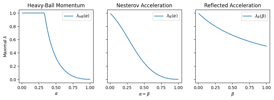
Figure 1: Upper bounds on $\lambda$ for Heavy-Ball (left), Nesterov (center) and Reflected (right) acceleration.

Extending by continuity, the constraint can be written explicitly in the general case as

$$\lambda<\lambda(\alpha,\beta):=\frac{\sqrt{(1-3\alpha)^{2}+4\beta(1+\beta)(1-\alpha)^{2}}-1+\alpha-2\alpha^{2}}{2(\beta-\alpha)(1+\alpha+\beta)}.$$

The function $(\alpha,\beta)\mapsto\lambda(\alpha,\beta)$ is shown in Figure 2.

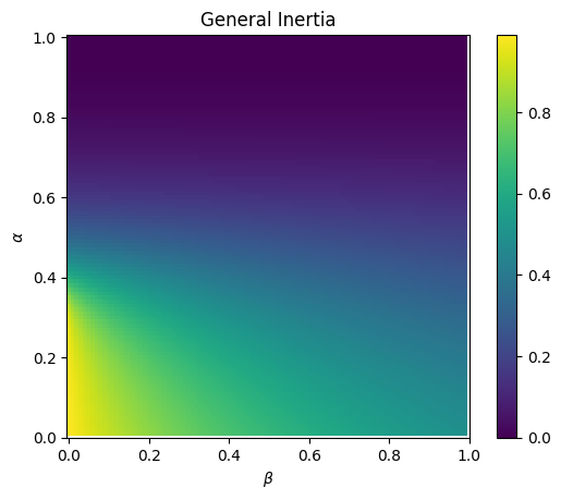
Figure 2: Upper bounds on $\lambda$ for general inertia as a function of $(\alpha,\beta)$.

3.2 Our Results in Perspective

Convergence of inertial methods has been studied by a number of researchers in different, and mostly less general contexts. We discuss here how the results established above relate to previously known ones.

3.2.1 Exact Methods

Several special cases of (1) in the unperturbed case $\varepsilon_{k}\equiv\rho_{k}\equiv\theta_{k}\equiv 0$ have already been studied, namely:

$\bullet$ Nesterov’s acceleration corresponds to $\alpha_{k}=\beta_{k}$. Weak convergence has been established in lorenz2015inertial for the forward-backward method, assuming square-summability of the residuals. This hypothesis was proved unnecessary in iutzeler2019generic , and convergence was proved under hypotheses equivalent to ours in the constant case. Also, (boct2015inertial, , Theorem 5), (shehu2018convergence, , Theorem 3.1) and (Dong, , Proposition 3.1 and Theorem 3.1), show weak convergence under hypotheses on the parameters that are similar, but more involved. Indeed, the author of Dong remarks that these conditions are too complicated to determine an upper bound for the inertial sequence in a simple way, even if the coefficient $\lambda_{k}$ is known. Moreover, in the case of $\lambda_{k}\equiv 0.5$, they are undesirably restrictive. The said hypotheses were simplified in (iyiola2021new, , Theorem 2.1), but are still more restrictive than ours. All of the above consider $T_{k}\equiv T$, with $T$ nonexpansive. The case of a family of operators was studied in (mainge2008convergence, , Theorems 3.1 and 3.2), both in the nonexpansive and in the firmly quasi-nonexpansive cases, but also assuming a summability condition on the residuals, which we have proved, based on the arguments in FierroMaulenPeypouquet , to be unnecessary, even under perturbations. On a different note, Nesterov’s acceleration has also been added to algorithms of extragradient type (thong2018inertial, , Theorems 3.1 and 3.2).

$\bullet$ The case $\beta_{k}\equiv 0$ (Heavy Ball momentum), was studied in alvarez2001inertial ; AccKM , where convergence is obtained assuming square-summability and boundedness of the residuals, respectively, both impractical hypotheses. This was solved in (dong2022new, , Theorem 1), where convergence is proved under assumptions similar to ours.

$\bullet$ Reflected acceleration, which corresponds to $\alpha_{k}\equiv 0$, was studied in (Dong2018, , Theorem 4) and (Dong2022, , Theorem 5.4), under slightly stronger assumptions on the parameters. The very particular case $\beta_{k}\equiv 1$ was analysed in (doi:10.1080/10556788.2021.1924715, , Theorem 3.1). On the other hand, (moudafi2018reflected, , Proposition 2.1) includes an additional projection step. Weak convergence is obtained for Lipschitz pseudo-contrative mappings, and strong convergence for Lipschitz strongly monotone mappings with monotonicity constant strictly larger than $1$.

$\bullet$ In the remaining cases (although still considering $\varepsilon_{k}\equiv\rho_{k}\equiv\theta_{k}\equiv 0$ and $T_{k}\equiv T$), weak convergence of Algorithm (1) was established in (Dong2018, , Theorem 1) and (Dong2022, , Theorem 5.1), assuming that $(\lambda_{k})$ is constant, both $(\alpha_{k})$ and $(\beta_{k})$ are nondecreasing, and an additional condition (in line with boct2015inertial ; shehu2018convergence ; Dong ), which the authors qualify as complicated and restrictive, in Dong2022 . An online selection of the relaxation parameters is studied in (dong2021general, , Theorem 3). Much stronger hypotheses (on the parameters, the operator and the residuals) are used in (gebregiorgis2023convergence, , Theorem 2). An application to three-operator splitting is given in (wen2019two, , Theorem 1), under ad hoc assumptions. Finally, a multi-step inertial Krasnoselskii-Mann algorithm is studied in (dong2019mikm, , Theorem 4.1), but also assuming summability of the residuals.

3.2.2 Perturbed Algorithms

For Nesterov’s acceleration, convergence under $\ell^{1}$ perturbations in the Krasnoselskii-Mann step is proved in (cui2019convergence, , Theorem 3.1). However, they assume the sequence $(x_{k})$ to be bounded, which is impractical and, as we show, unnecessary. Similar results were obtained earlier in (khatibzadeh2015inexact, , Theorems 3.5 and 5.1), assuming both that the generated sequence is bounded and that the residuals are square-summable. An inexact version of FISTA was analyzed in (attouch2018fast, , Theorem 5.1) without any boundedness hypotheses, but assuming that the perturbations satisfy the summability condition $\sum k\|\varepsilon_{k}\|<+\infty$, which is stronger than ours. Relative error conditions have been accounted for in (padcharoen2019convergence, , Theorem 3.1), (alves2020relative, , Theorem 3.6) and (alves2020relativeb, , Theorem 2.5, 3.3 and 4.4), as well as (ezeora2022inexact, , Theorems 3.2 and 3.3), although the latter is concerned with alternated inertia. Other approaches include (aujol2015stability, , Algorithm 1), as well as an inexact multilayer FISTA (lauga2023multilevel, , Algorithm 2.1) and an inexact accelerated forward-backward algorithm (villa2013accelerated, , Theorem 3.2), where the summability conditions on the perturbations are taylored to the corresponding methods.

3.3 Operators Not Sharing a Fixed Point

Our results can also be applied when $\bigcap_{k\geq 1}\mathrm{Fix}(T_{k})=\emptyset$, if instead we are interested in the Kuratowski lower limit of the family $\big{(}\mathrm{Fix}(T_{k})\big{)}$. This set, which we denote by $F_{\infty}$, consists of all $p_{\infty}\in\mathcal{H}$ for which there is a sequence $(p_{k})$, such that $p_{k}\in\mathrm{Fix}(T_{k})$ for all $k\geq 1$, and $p_{k}\to p_{\infty}$.

To this end, first fix $p_{\infty}\in F_{\infty}$, and set $p_{k}=\text{Proj}_{\mathrm{Fix}(T_{k})}p_{\infty}$. For each $k$, define $\tilde{T}_{k}\colon\mathcal{H}\to\mathcal{H}$ by

$$\tilde{T}_{k}x=T_{k}(x+p_{k}-p_{\infty})-p_{k}+p_{\infty}.$$ (19)

Clearly, $p_{\infty}\in\tilde{F}\coloneqq\bigcap_{k\geq 1}\mathrm{Fix}(\tilde{T}_{k})$, so $\mathrm{Fix}(\tilde{T}_{k})\neq\emptyset$, and $\tilde{p}_{k}\in\mathrm{Fix}(\tilde{T}_{k})$ if, and only if, $\tilde{p}_{k}+p_{k}-p_{\infty}\in\mathrm{Fix}(T_{k})$. Since $T_{k}$ is quasi-nonexpansive, for each $x\in\mathcal{H}$, we have

$$\|\tilde{T}_{k}x-\tilde{p}_{k}\|=\|T_{k}(x+p_{k}-p_{\infty})-(\tilde{p}_{k}+p_{k}-p_{\infty})\|\leq\|(x+p_{k}-p_{\infty})-(\tilde{p}_{k}+p_{k}-p_{\infty})\|=\|x-\tilde{p}_{k}\|,$$

and so, $\tilde{T}_{k}$ is quasi-nonexpansive, as well. Quasi-contractivity is also inherited by $\tilde{T}_{k}$ from $T_{k}$.

By setting $\tilde{x}_{k}=x_{k}-p_{k-1}+p_{\infty}$, $\tilde{y}_{k}=y_{k}-p_{k}+p_{\infty}$, and $\tilde{z}_{k}=z_{k}-p_{k}+p_{\infty}$, Algorithm (1) becomes

$$\begin{cases}\tilde{y}_{k}&=\quad\tilde{x}_{k}+\alpha_{k}(\tilde{x}_{k}-\tilde{x}_{k-1})+\tilde{\varepsilon}_{k},\qquad\hbox{where}\qquad\tilde{\varepsilon}_{k}:=p_{k-1}-p_{k}+\alpha_{k}(p_{k-1}-p_{k-2})+\varepsilon_{k}\\ \tilde{z}_{k}&=\quad\tilde{x}_{k}+\beta_{k}(\tilde{x}_{k}-\tilde{x}_{k-1})+\tilde{\rho}_{k},\qquad\hbox{where}\qquad\tilde{\rho}_{k}:=p_{k-1}-p_{k}+\beta_{k}(p_{k-1}-p_{k-2})+\rho_{k}\\ \tilde{x}_{k+1}&=\quad(1-\lambda_{k})\tilde{y}_{k}+\lambda_{k}\tilde{T}_{k}\tilde{z}_{k}+\theta_{k}.\end{cases}$$

If $(\varepsilon_{k}),(\rho_{k}),(p_{k}-p_{k-1})\in\ell^{p}(\mathcal{H})$, then also $(\tilde{\varepsilon}_{k}),(\tilde{\rho}_{k})\in\ell^{p}(\mathcal{H})$.

Remark 6

It is neither necessary to know $p_{\infty}$ and the sequence $(p_{k})$, nor to construct the operators $\tilde{T}_{k}$ and the auxiliary variables $\tilde{x}_{k}$, $\tilde{y}_{k}$ or $\tilde{z}_{k}$. These are merely artifacts to prove convergence.

Proposition 1 shows that $\lim_{k\to\infty}\|\tilde{x}_{k}-\tilde{x}_{k-1}\|=\lim_{k\to\infty}\|\tilde{T}_{k}\tilde{z}_{k}-\tilde{y}_{k}\|=0$, and $\lim_{k\to\infty}\|\tilde{x}_{k}-p_{\infty}\|$ exists. As a consequence, $\lim_{k\to\infty}\|x_{k}-x_{k-1}\|=\lim_{k\to\infty}\|T_{k}z_{k}-z_{k}\|=0$ (because $\lim_{k\to\infty}\|z_{k}-y_{k}\|=0$), and $\lim_{k\to\infty}\|x_{k}-p_{\infty}\|$ exists. This is true for each $p_{\infty}\in F_{\infty}$.

Let us say that $(T_{k})$ nicely approximates $F_{\infty}$ if $u_{k}\rightharpoonup u$ and $T_{k}u_{k}-u_{k}\to 0$ together imply $u\in F_{\infty}$.

In $\mathcal{H}=\mathbb{R}^{N}$, this holds if there is a strictly increasing continuous function $\Phi:\mathbb{R}\to\mathbb{R}$ such that $\Phi(0)=0$ and

$$\text{dist}\big{(}z,\mathrm{Fix}(T_{k})\big{)}\leq\Phi\big{(}\|z-T_{k}z\|\big{)}$$

for every $k\geq 1$, and $z\in\mathcal{H}$. This is similar to the error bound in Luo_Tseng , and can also be understood as the family $(\varphi_{k})$ of functions, defined by $\varphi_{k}(z)=\|z-T_{k}z\|$, having a common residual function $\Phi$ (see (bolte2017error, , Section 2.4)).

Proceeding as in the proof of Theorem 2.1, we obtain:

Proposition 2

Let $T_{k}\colon\mathcal{H}\to\mathcal{H}$ be a family of quasi-nonexpansive operators that nicely approximates $F_{\infty}\neq\emptyset$. Let Hypothesis 2.1 and Inequality (7) hold, and assume the error sequences $(\varepsilon_{k})$, $(\rho_{k})$, and $(\theta_{k})$ belong to $\ell^{1}(\mathcal{H})$. Assume moreover that there exists a sequence $(p_{k})$ with $p_{k}\in\mathrm{Fix}(T_{k})$ and $(p_{k}-p_{k-1})\in\ell^{1}(\mathcal{H})$. If $(x_{k},y_{k},z_{k})$ is generated by Algorithm (1), then $(x_{k},y_{k},z_{k})$ converges weakly to some $(p^{*},p^{*},p^{*})$, with $p^{*}\in F_{\infty}$.

The preceding discussion also allows us to prove the following:

Proposition 3

Let $T_{k}\colon\mathcal{H}\to\mathcal{H}$ be a family of $q_{k}$-quasi-contractive operators with $q_{k}\leq q<1$, and such that $\mathrm{Fix}(T_{k})=\{p_{k}\}$, with $p_{k}\to p^{*}$ and $(p_{k}-p_{k-1})\in\ell^{2}(\mathcal{H})$. Let Hypothesis 2.1 and Inequality (11) hold, and assume the error sequences $(\varepsilon_{k})$, $(\rho_{k})$, and $(\theta_{k})$ belong to $\ell^{2}(\mathcal{H})$. If $(x_{k},y_{k},z_{k})$ is generated by Algorithm (1), then $(x_{k},y_{k},z_{k})$ converges strongly to $(p^{*},p^{*},p^{*})$. Moreover, $\sum_{k=1}^{\infty}\|x_{k}-p^{*}\|^{2}<\infty$.

4 Numerical Results

In this section, we illustrate how the different popular acceleration schemes behave in two examples. In Section 4.1, we look into the image inpainting problem, using the three operator scheme. Secondly, in Section 4.2, we consider a Nash-Cournot oligopolistic equilibrium model in electricity markets.

The experiments are implemented in Python 3.11.5, running on a laptop with Intel Quad-Core i7-1068NG7 at 2.3 GHz and 16 GB of RAM.

4.1 Image Inpainting Problem

For $A,B\colon\mathcal{H}\rightrightarrows\mathcal{H}$ maximally monotone operators and $C\colon\mathcal{H}\to\mathcal{H}$ a $\tau$-cocoercive operator, we aim to find $\hat{x}\in\mathcal{H}$ such that

$$\hat{x}\in\text{Zer}(A+B+C).$$ (20)

Such a scheme is called a three-operator splitting scheme DavisYin , and is equivalent to finding $\bigcap_{k\geq 1}\mathrm{Fix}(T_{k})$, where $T_{k}$ is defined as

$$T_{k}\coloneqq I-J_{\rho_{k}B}+J_{\rho_{k}A}\circ(2J_{\rho_{k}B}-I-\rho_{k}C\circ J_{\rho_{k}B}).$$

Indeed, $J_{\rho_{k}B}(\mathrm{Fix}(T_{k}))=\text{Zer}(A+B+C)$, and the operator $T_{k}$ is nonexpansive when $(\rho_{k})\subset(0,2\tau)$. As such, Algorithm 1 converges under the given conditions.

Consider the image inpainting problem: We represent an image $X$ of $M$ by $N$ pixels by a tensor in $\mathcal{H}\coloneqq[0,1]^{M\times N\times 3}$, in which the three layers represent the red, green and blue colour channels. Let $\Omega$ be an element of $\{0,1\}^{M\times N}$ such that $\Omega_{ij}=0$ indicates that the pixel at position $(i,j)$, on all colour channels, has been damaged. Denote by $\mathcal{A}$ the linear operator that maps an image to an image whose elements in $\Omega$ have been erased. More precisely,

$$\mathcal{A}\colon\mathcal{H}\to\mathcal{H},\quad X\mapsto\tilde{X},\quad\text{where }\tilde{X}_{ijk}=\Omega_{ij}\cdot X_{ijk}.$$

The operator $\mathcal{A}$ is a self-adjoint bounded projection map with operator norm $1$. We denote the damaged image by $X_{\text{corrupt}}=\mathcal{A}X$. The objective is to recover an image from $X_{\text{corrupt}}$ that mainly overlaps on the points where $\Omega_{ij}=1$, and which looks better to the eye, which is obtained by adding the regularization $\|X_{(1)}\|_{*}+\|X_{(2)}\|_{*}$, where $X_{(1)}\coloneqq[X_{\cdot\cdot 1}~{}X_{\cdot\cdot 2}~{}X_{\cdot\cdot 3}]$, $X_{(2)}\coloneqq\left[X_{\cdot\cdot 1}^{T}~{}X_{\cdot\cdot 2}^{T}~{}X_{\cdot\cdot 3}^{T}\right]^{T}$ and $\|\cdot\|_{*}$ denotes the nuclear norm. The image inpainting problem is

$$\min_{X\in\mathcal{H}}\left\{\frac{1}{2}\|\mathcal{A}X-X_{\text{corrupt}}\|^{2}+\sigma\|X_{(1)}\|_{*}+\sigma\|X_{(2)}\|_{*}\right\},$$ (21)

where $\sigma>0$ is a regularisation parameter. This problem can be described by (20). To this end, first write $f(X)=\sigma\|X_{(1)}\|_{*}$, $g(X)=\sigma\|X_{(2)}\|_{*}$, $h(X)=\frac{1}{2}\|X-X_{\text{corrupt}}\|^{2}$ and $L=\mathcal{A}$. Then, set $A\coloneqq\partial f$, $B\coloneqq\partial g$, both maximally monotone, and $C\coloneqq\nabla(h\circ L)$, which is $\tau/\|L\|_{\text{op}}$-cocoercive.

The image to be inpainted has dimensions $512\times 512$ pixels. We select a regularisation parameter of $\sigma=0.5$, a tolerance of $\varepsilon=10^{-3}$, and the error function $\mathcal{R}\colon\mathcal{H}\times\mathcal{H}\to\mathbb{R}_{+}$ defined by

$$\mathcal{R}(X_{k},X_{k-1})=\frac{\|X_{k}-X_{k-1}\|}{\|X_{k-1}\|}.$$ (22)

We corrupt the images randomly, with a certain percentage of pixels erased. To ensure the termination of the algorithm, we enforce a maximal number of iterations of $100$, after which we consider that the algorithm did not converge. We always set $X_{0}=X_{1}=X_{\text{corrupt}}$.

For simplicity, we set $\rho_{k}\equiv\rho\in(0,2)$ and $\lambda_{k}\equiv\lambda\in(0,1)$, and add no perturbations (other than possible rounding errors by the machine). We run multiple versions of the algorithm, corresponding to different inertial schemes: no inertia, Nesterov, Heavy Ball, and reflected. In each case, we pick $\alpha$ and $\beta$ such that Inequality (7) is tight, and then select

$$\alpha_{k}=\left(1-\frac{1}{k}\right)\alpha,\quad\beta_{k}=\left(1-\frac{1}{k}\right)\beta.$$

The Tests

First, we compare the evolution of the number of iterations and the execution time required by our algorithms to inpaint a randomly corrupted image, as a function of the percentage of pixels erased, whilst fixing the step size $\rho=1$ and the relaxation parameter $\lambda=0.5$. The results are shown in Figure 3. As could be expected, we observe an overall increasing trend. The Heavy Ball acceleration performs overall the best, and is capable of restoring the image with close to $80\%$ of its pixels erased in the given number of iterations, whereas the non-inertial version only is when at most $50\%$ are erased.

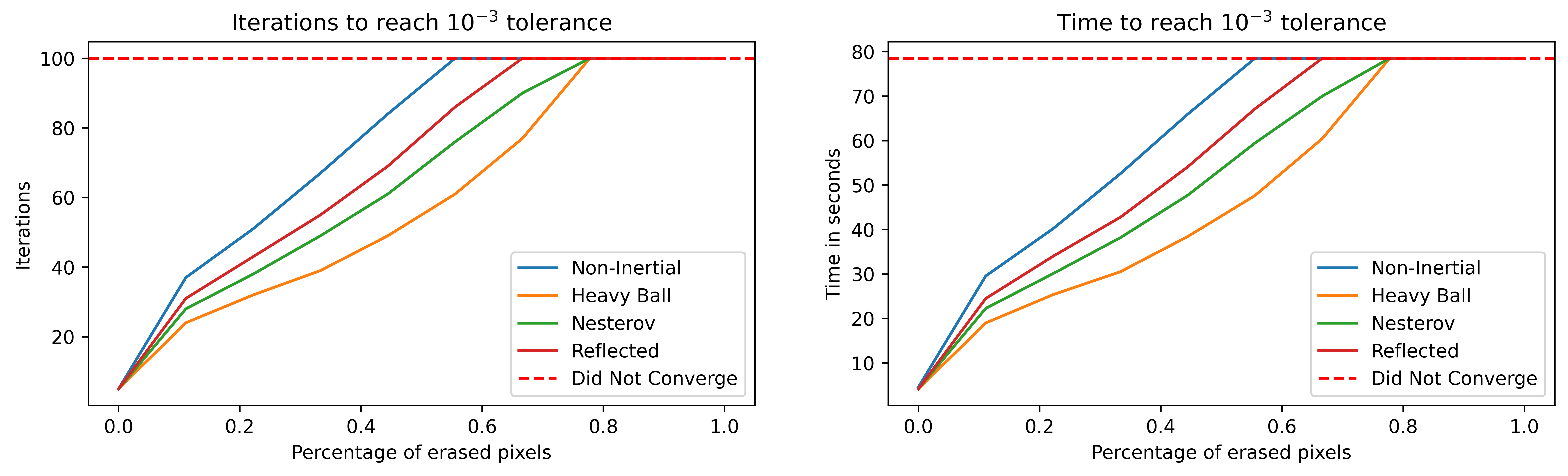
Figure 3: Number of iterations and execution time for different ratios of erased pixels, with $\rho=1$ and $\lambda=0.5$.

Next, we fix the relaxation parameter $\lambda=0.5$ and randomly corrupt $50\%$ of the pixels in the image. We iterate over representative values of the step size $\rho\in(0,2)$. The results are shown in Figure 4. Similar observations as for the percentage with respect to the comparison of the different versions may be made. Additionally, we notice that a larger value of $\rho$ accelerates the convergence.

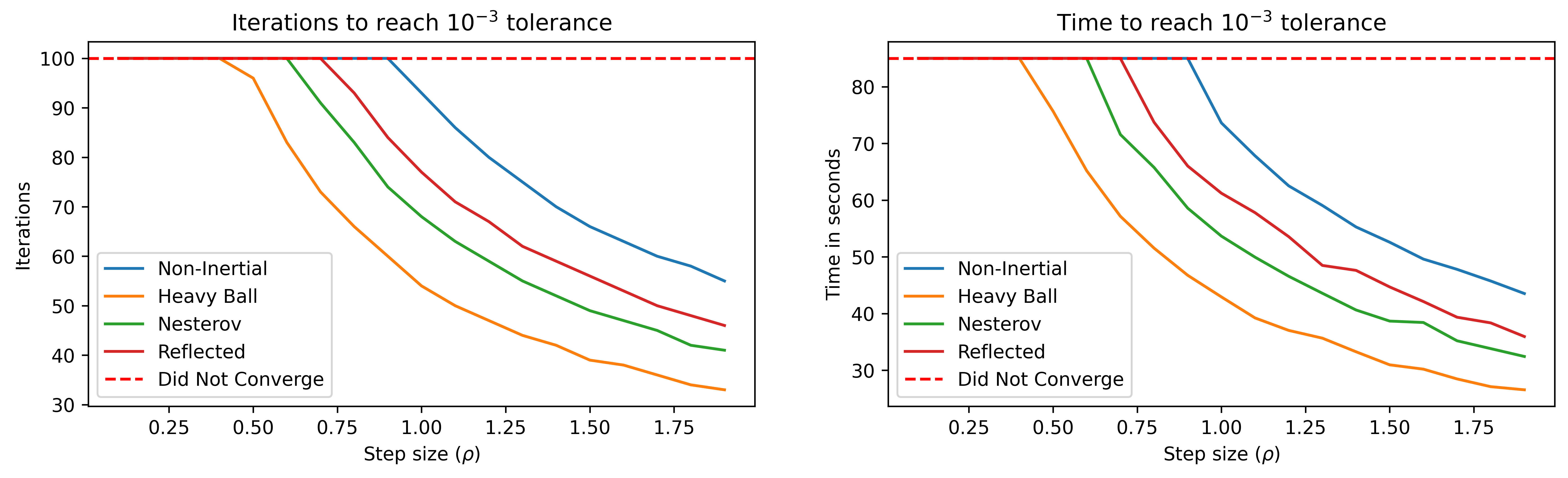
Figure 4: Number of iterations and execution time for $\lambda=0.5$ and a ratio of erased pixels of $50\%$, as a function of the step size $\rho$.

Finally, visual results for each version of the algorithm are shown in Figure 5, and the convergence rates in Figure 6. Here, we considered a corrupted image with $50\%$ of erased pixels, regularisation parameter $\sigma=0.5$, step size $\rho=1.8$, and relaxation parameter $\lambda=0.8$.

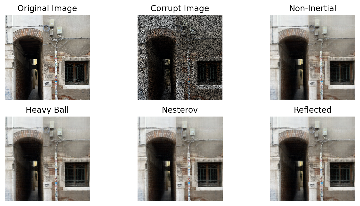
Figure 5: Inpainted image with $\lambda=0.8$, $\rho=1.8$, and $\sigma=0.5$.

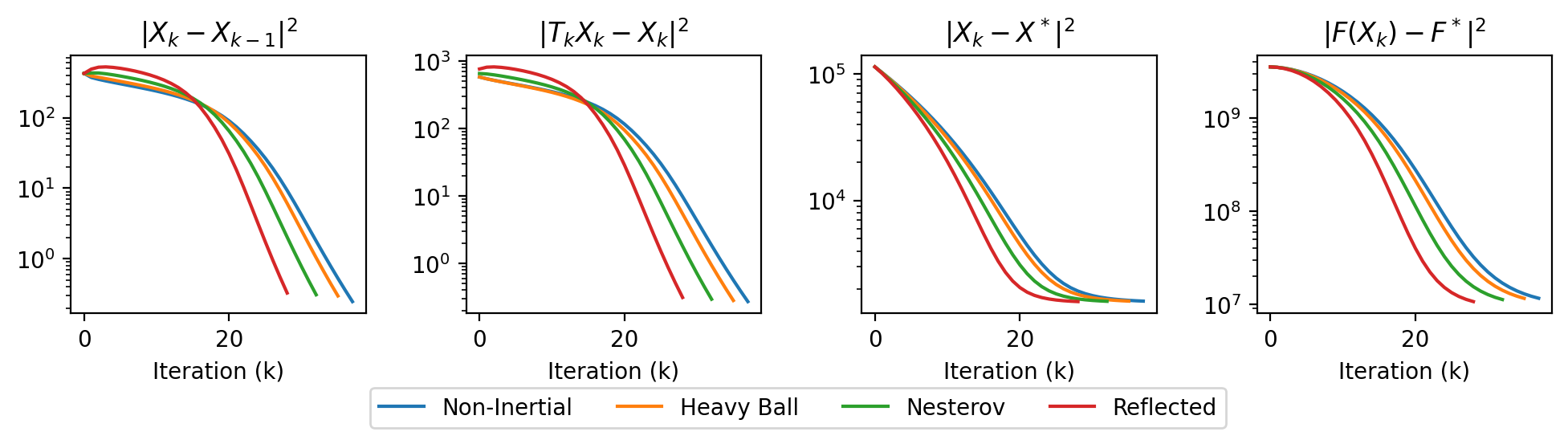
Figure 6: Convergence plots of the residuals of the iterations. $F$ is the objective function to be minimised, and $X^{*}$ and $F^{*}$ represent the minimiser and minimal value of $F$, respectively.

4.2 Nash-Cournot Equilibrium Model

We now consider a Nash-Cournot oligopolistic equilibrium model in electricity production markets contreras2004numerical . We consider $m$ companies, and denote by $x_{i}$ the power generated by company $i$. The generation price for company $i$ is $p_{i}(s)=\gamma-\beta_{i}\cdot s$, where $s=\sum_{i=1}^{m}x_{i}$. The profit made by company $i$ is $f_{i}(x)=p_{i}(s)x_{i}-c_{i}(x_{i})$, where $c_{i}(x_{i})$ is the cost to generate $x_{i}$ by company $i$. We denote $C_{i}$ the strategy set of company $i$ so that $x_{i}\in C_{i}$, and define the strategy profile set by $C=C_{1}\times\cdots\times C_{m}$.

In Cournot competition, no firms cooperate or collude–each company seeks to maximise their profit and assume the remaining firms do the same. A point $\hat{x}\in C$ is a Nash equilibrium if, for all $i=1,\ldots,m$,

$$f_{i}(\hat{x})=\max_{x_{i}\in C_{i}}f_{i}(\hat{x}[x_{i}]),$$

where $\hat{x}[x_{i}]$ represents the vector $\hat{x}$ whose $i$th component has been replaced by the entry $x_{i}$. This means that, under strategy profile $\hat{x}$, no single firm benefits from deviating from the strategy $\hat{x}$.

We define the Nikaido-Isoda pjm/1171984836 function $f\colon C\times C\to\mathbb{R}$ by $f(x,y)=\sum_{i=1}^{m}\left(f_{i}(x)-f_{i}(x[y_{i}])\right)$. We may now write the above problem as finding $\hat{x}\in C$ such that $f(\hat{x},x)\geq 0$ for all $x\in C$. Assuming the cost functions $c_{i}$ are convex and differentiable, this can be rewritten as yen2016algorithm

$$\langle F(\hat{x}),x-\hat{x}\rangle\geq 0\quad\forall x\in C,$$ (23)

where $F(x)=Bx-\Gamma+\nabla\phi(x)$ with

$$\Gamma\coloneqq(\gamma,\cdots,\gamma)^{T},\quad\tilde{B}\coloneqq\begin{pmatrix}\beta_{1}&0&\cdots&0\\ 0&\beta_{2}&\cdots&0\\ \vdots&\vdots&\ddots&\vdots\\ 0&0&\cdots&\beta_{m}\\ \end{pmatrix},\quad B\coloneqq\begin{pmatrix}0&\beta_{1}&\cdots&\beta_{1}\\ \beta_{2}&0&\cdots&\beta_{2}\\ \vdots&\vdots&\ddots&\vdots\\ \beta_{m}&\beta_{m}&\cdots&0\\ \end{pmatrix},\quad\phi(x)\coloneqq x^{T}\tilde{B}x+\sum_{i=1}^{m}c_{i}(x_{i}).$$

Variational inequality problems such as Problem (23) where $C$ is a nonempty, closed and convex set and $F$ is monotone and $L$-Lipschitz have been extensively studied xu2010iterative ; malitsky2015projected ; he2018selective ; zhao2018iterative ; yao2019convergence ; dong2021two . The simplest iterative procedure to solve the above variational inequality is through the projected gradient method, namely

$$x_{k+1}=P_{C}(x_{n}-\rho F(x_{n})),$$

where $P_{C}\colon\mathcal{H}\to C$ represents the projection onto $C$. By writing $T_{n}\equiv T=P_{C}(I-\rho F)$, we obtain a family of nonexpansive operators whose fixed points represent a solution to Problem (23), provided that the step size $\rho$ satisfies $0<\rho<2/L$ xu2010iterative . We notice that the method by Malitsky malitsky2015projected is a reflected acceleration of the previous, with parameter $\beta_{n}\equiv 1$.

We shall assume the cost functions are quadratic, namely of the form

$$c_{i}(x_{i})=\frac{1}{2}p_{i}x_{i}^{2}+q_{i}x_{i},$$

where $p_{i}>0$ such that $L=\|B-p^{T}I\|$, where $p=(p_{1},\ldots,p_{m})^{T}$. The parameters $\beta_{i},p_{i},q_{i}$ are selected uniformly at random in the intervals $(0,1]$, $[1,3]$ and $[1,3]$ respectively, and we assume $C_{i}=[1,40]$, for all $1\leq i\leq m$. We set $m=8$, $\gamma=200$ and $\rho=1/L$. We set a stopping criteria based on the error function given by (22), and select a tolerance of $\varepsilon=10^{-4}$ and a maximum number of iterations of $400$.

As in the previous example, we run multiple versions of the algorithm, corresponding to the different types of inertia, no perturbations and $\alpha_{k},\beta_{k}$ chosen as before.

The Tests

We run the algorithm for various values of the relaxation parameter $\lambda\in(0,1)$. We observe convergence for all the selected values of $\lambda$, and faster convergence for all methods as $\lambda\approx 1$. The Heavy Ball acceleration produces the best results, and the required number of iterations are roughly identical for $\lambda\geq 0.2$. The results are depicted in Figure 7.

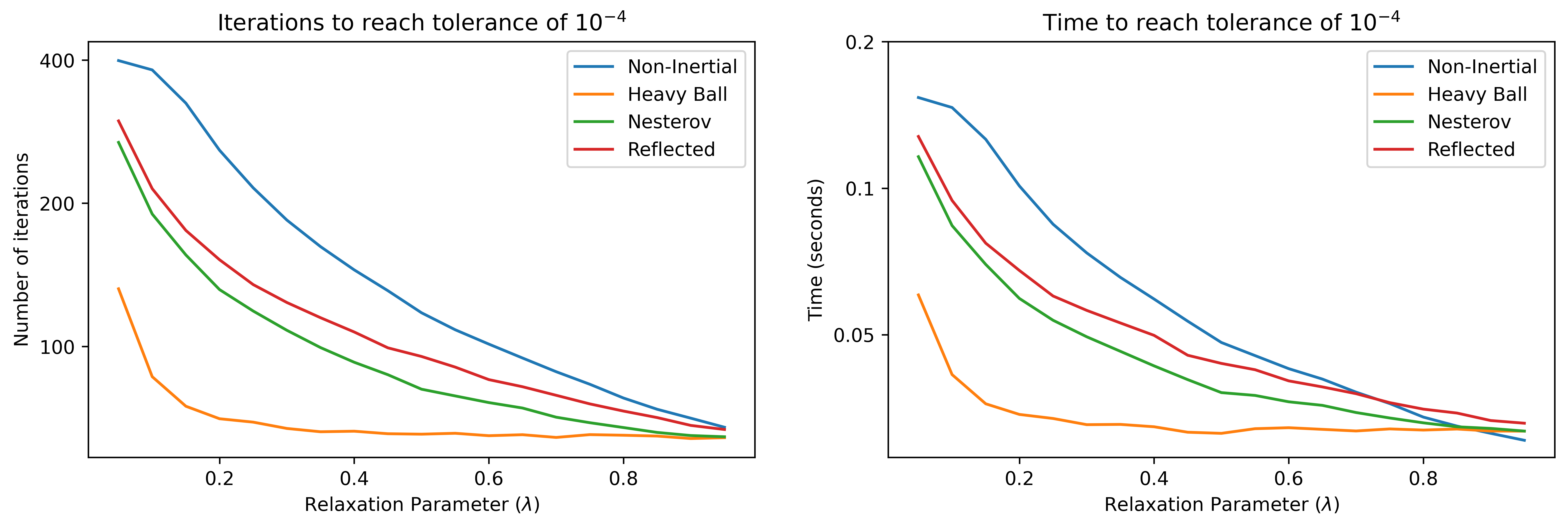
Figure 7: Variation of the relaxation parameter $\lambda$ for $\rho=1/L$.

We fix the relaxation parameter to be $\lambda=0.5$, and execute the algorithm for various step-sizes $\rho\in(0,2/L)$. The convergence results are plotted in Figure 8.

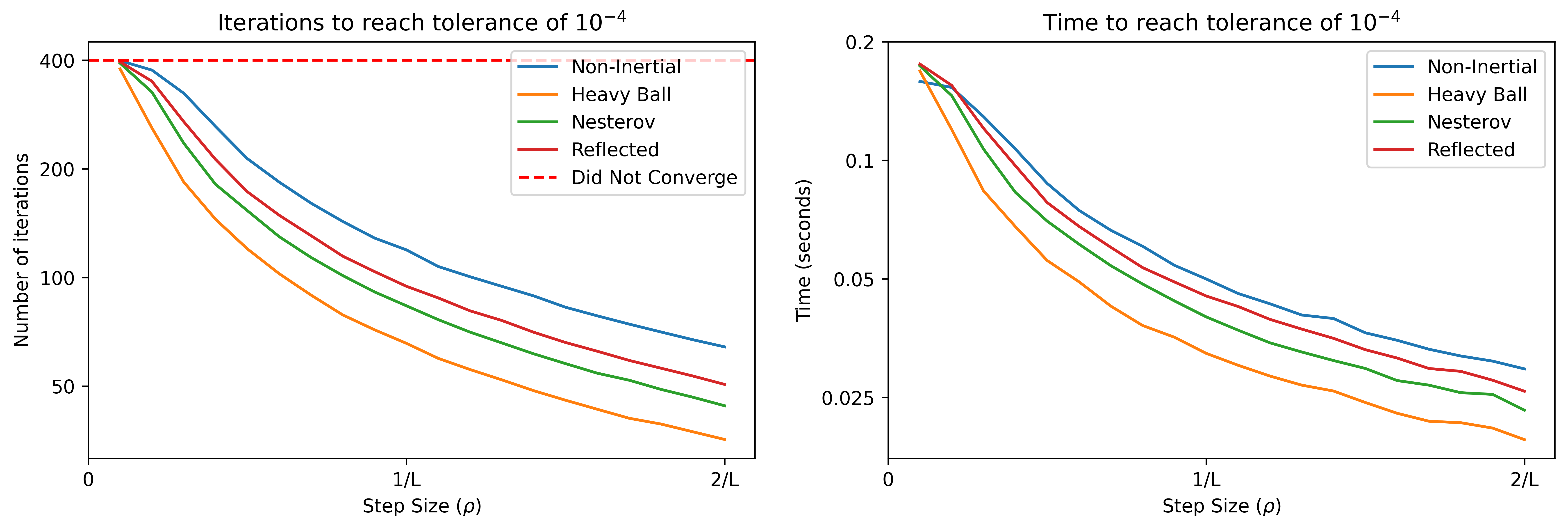
Figure 8: Variation of the step size $\rho\in(0,2/L)$ for $\lambda=0.5$.

Figure 9 shows convergence rates of the residual quantities, using the parameters $\rho=\frac{2}{L}$ and $\lambda=0.8$, observed favorable throughout the previous two experiments. As expected, we do observe linear convergence asymptotically.

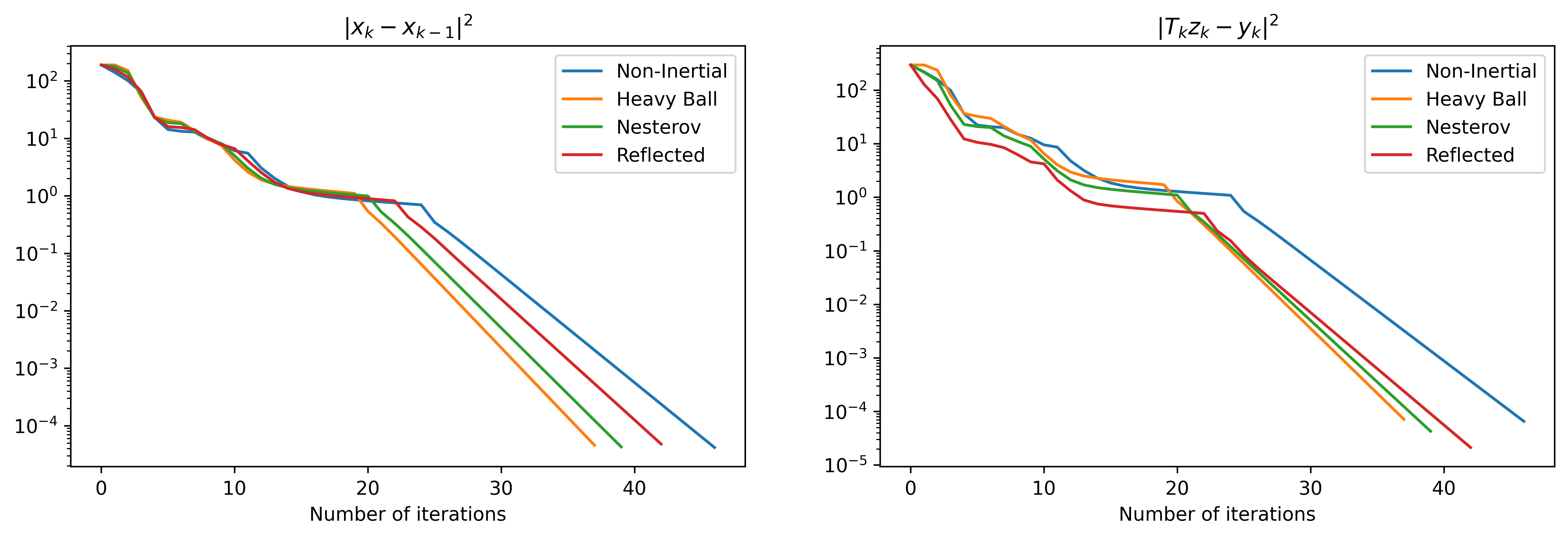
Figure 9: Convergence plots of the residuals for $\rho=2/L$ and $\lambda=0.8$.

Appendix A Appendix

The following properties of the norm were used repeatedly in Section 2. The first one is a generalized parallelogram identity:

Lemma 2

For every $u,v\in\mathcal{H}$ and $\zeta\in\mathbb{R}$, we have

$$\|u+\zeta v\|^{2}=(1+\zeta)\|u\|^{2}+\zeta(1+\zeta)\|v\|^{2}-\zeta\|u-v\|^{2}.$$

Proof

It suffices to add the identities

$$\|u+\zeta v\|^{2} = \|u\|^{2}+\zeta^{2}\|v\|^{2}+2\zeta\langle u,v\rangle$$

$$\zeta\|u-v\|^{2} = \zeta\|u\|^{2}+\zeta\|v\|^{2}-2\zeta\langle u,v\rangle$$

and rearrange the terms.

The next one is a direct consequence of Cauchy-Schwarz and Young’s inequalities:

Lemma 3

For every $u,v\in\mathcal{H}$ and $\gamma>0$, we have

$$\left(1-\gamma\right)\|u\|^{2}+\left(1-\frac{1}{\gamma}\right)\|v\|^{2}\leq\|u\pm v\|^{2}\leq\left(1+\gamma\right)\|u\|^{2}+\left(1+\frac{1}{\gamma}\right)\|v\|^{2}.$$

Proof

We first bound

$$\left|\frac{}{}\!\|u\pm v\|^{2}-\|u\|^{2}-\|v\|^{2}\right|=2|\langle u,v\rangle|\leq 2\left(\frac{}{}\!\sqrt{\gamma}\|u\|\right)\left(\frac{1}{\sqrt{\gamma}}\|v\|\right)\leq\gamma\|u\|^{2}+\frac{1}{\gamma}\|v\|^{2},$$

and then rewrite without the absolute value.

We now provide two elementary but not so standard results on real sequences that have been used in Section 2. The first one is an extension of (attouch2018fast, , Lemma 5.14).

Lemma 4

Let $(\zeta_{k})$ be a nonnegative sequence such that

$$\zeta_{j+1}^{2}-M\zeta_{j}^{2}\leq C+\sum_{k=1}^{j}\sum_{i=0}^{k+1}e_{k,i}\zeta_{i},$$ (24)

where $C\geq 0$, $0\leq M<1$ and $e_{k,i}\geq 0$, with $D:=\sum_{k=1}^{\infty}\sum_{i=0}^{k+1}e_{k,i}<\infty$ for each $i$. Then, $(\zeta_{j})$ is bounded.

Proof

Set $Z_{j}=\max_{i=1,\dots j}\zeta_{i}$. Take $n\geq 1$. For every $j\leq n$, (24) gives

$$\zeta_{j+1}^{2}\leq MZ_{n}^{2}+C+Z_{n+1}\sum_{k=1}^{j}\sum_{i=0}^{k+1}e_{k,i}\leq MZ_{n+1}^{2}+C+DZ_{n+1}.$$

Since the right-hand side does not depend on $j$, we may take the maximum for $j=1,\dots,n$, and rearrange the terms, to obtain

$$(1-M)Z_{n+1}^{2}-DZ_{n+1}-C\leq 0,$$

which implies $(\zeta_{j})$ is bounded.

Now, write $[\omega]_{+}=\max\{0,\omega\}$ for $\omega\in\mathbb{R}$. The following result is a straightforward extension of (mainge2008convergence, , Lemma 2.2), a result that was actually established much earlier, embedded in the proof of (alvarez2001inertial, , Theorem 2.1).

Lemma 5

Let $(a_{k})$ and $(d_{k})$ be nonnegative sequences such that $a_{k}\leq a<1$ for all $k\geq 0$, and $\sum_{k=0}^{\infty}d_{k}<+\infty$. Consider a real sequence $(\Omega_{k})$ such that

$$\Omega_{k+1}\leq a_{k}\Omega_{k}+d_{k}$$

for all $k\geq 0$. Then $\sum_{k=1}^{\infty}[\Omega_{k}]_{+}$ is convergent. If, moreover, $d_{k}\equiv 0$, then $[\Omega_{k+1}]_{+}\leq a^{k}[\Omega_{1}]_{+}$. Either way, if $\Omega_{k}\geq\omega_{k}-b\omega_{k-1}$ for all $k\geq 0$, where $b\in[0,1]$ and $(\omega_{k})$ is nonnegative, then $(\omega_{k})$ is convergent. If, moreover, $b<1$, then $\sum_{k=0}^{\infty}\omega_{k}<+\infty$.

References

- [1] Felipe Alvarez and Hedy Attouch. An inertial proximal method for maximal monotone operators via discretization of a nonlinear oscillator with damping. Set-Valued Analysis, 9:3–11, 2001.
- [2] Maicon Marques Alves, Jonathan Eckstein, Marina Geremia, and Jefferson G. Melo. Relative-error inertial-relaxed inexact versions of Douglas-Rachford and ADMM splitting algorithms. Computational Optimization and Applications, 75:389–422, 2020.
- [3] Maicon Marques Alves, Marina Geremia, and Raul T. Marcavillaca. A relative-error inertial-relaxed inexact projective splitting algorithm. arXiv preprint arXiv:2002.07878, 2020.
- [4] Hedy Attouch, Zaki Chbani, Juan Peypouquet, and Patrick Redont. Fast convergence of inertial dynamics and algorithms with asymptotic vanishing viscosity. Mathematical Programming, 168:123–175, 2018.
- [5] Hédy Attouch, Marc-Olivier Czarnecki, and Juan Peypouquet. Coupling forward-backward with penalty schemes and parallel splitting for constrained variational inequalities. SIAM Journal on Optimization, 21(4):1251–1274, 2011.
- [6] Hédy Attouch, Marc-Olivier Czarnecki, and Juan Peypouquet. Prox-penalization and splitting methods for constrained variational problems. SIAM Journal on Optimization, 21(1):149–173, 2011.
- [7] Jean-François Aujol and Charles H. Dossal. Stability of over-relaxations for the forward-backward algorithm, application to FISTA. SIAM Journal on Optimization, 25(4):2408–2433, 2015.
- [8] Amir Beck and Marc Teboulle. A fast iterative shrinkage-thresholding algorithm for linear inverse problems. SIAM journal on imaging sciences, 2(1):183–202, 2009.
- [9] Jérôme Bolte, Trong Phong Nguyen, Juan Peypouquet, and Bruce W Suter. From error bounds to the complexity of first-order descent methods for convex functions. Mathematical Programming, 165:471–507, 2017.
- [10] Radu Ioan Boţ, Ernö Robert Csetnek, and Christopher Hendrich. Inertial Douglas–Rachford splitting for monotone inclusion problems. Applied Mathematics and Computation, 256:472–487, 2015.
- [11] Yair Censor. Superiorization: The asymmetric roles of feasibility-seeking and objective function reduction. arXiv preprint arXiv:2212.14724, 2022.
- [12] Javier Contreras, Matthias Klusch, and Jacek B Krawczyk. Numerical solutions to Nash-Cournot equilibria in coupled constraint electricity markets. IEEE Transactions on Power Systems, 19(1):195–206, 2004.
- [13] Fuying Cui, Yang Yang, Yuchao Tang, and Chuanxi Zhu. Convergence analysis of an inexact inertial Krasnoselskii-Mann algorithm with applications. arXiv preprint arXiv:1908.11029, 2019.
- [14] Damek Davis and Wotao Yin. A Three-Operator Splitting Scheme and its Optimization Applications. Set-Valued and Variational Analysis, 25:829–858, 2017.
- [15] Qiao-Li Dong, Yeol Je Cho, Songnian He, Panos M. Pardalos, and Themistocles M. Rassias. The Inertial Krasnosel’skii–Mann Iteration, pages 59–73. Springer International Publishing, Cham, 2022.
- [16] Qiao-Li Dong, Yeol Je Cho, and Themistocles M. Rassias. Applications of Nonlinear Analysis, chapter General Inertial Mann Algorithms and Their Convergence Analysis for Nonexpansive Mappings, pages 175–191. Springer International Publishing, Cham, 2018.
- [17] Qiao-Li Dong, Songnian He, and Lulu Liu. A general inertial projected gradient method for variational inequality problems. Computational and Applied Mathematics, 40(5):168, 2021.
- [18] Qiao-Li Dong, JZ Huang, XH Li, YJ Cho, and Th M Rassias. MiKM: multi-step inertial Krasnosel’skiǐ–Mann algorithm and its applications. Journal of Global Optimization, 73:801–824, 2019.
- [19] Qiao-Li Dong, Xiao-Huan Li, and Themistocles M Rassias. Two projection algorithms for a class of split feasibility problems with jointly constrained nash equilibrium models. Optimization, 70(4):871–897, 2021.
- [20] Qiao-Li Dong and Hb. Yuan. Accelerated Mann and CQ algorithms for finding a fixed point of a nonexpansive mapping. Fixed Point Theory and Applications, 125, 2015.
- [21] Yunda Dong. New inertial factors of the Krasnoselskii-Mann iteration. Set-Valued and Variational Analysis, 29:145–161, 2021.
- [22] Yunda Dong and Mengdi Sun. New Acceleration Factors of the Krasnosel’skiĭ-Mann Iteration. Results in Mathematics, 77(5):194, 2022.
- [23] Jeremiah N. Ezeora and Frank E. Bazuaye. Inexact generalized proximal point algorithm with alternating inertial steps for monotone inclusion problem. Advances in Fixed Point Theory, 12(6), 2022.
- [24] Solomon Gebregiorgis and Poom Kumam. Convergence results on the general inertial Mann–Halpern and general inertial Mann algorithms. Fixed Point Theory and Algorithms for Sciences and Engineering, 2023(1):18, 2023.
- [25] C.W Groetsch. A note on segmenting Mann iterates. Journal of Mathematical Analysis and Applications, 40(2):369–372, 1972.
- [26] Osman Güler. New Proximal Point Algorithms for Convex Minimization. SIAM Journal on Optimization, 2(4):649–664, 1992.
- [27] Songnian He, Hanlin Tian, and Hong-Kun Xu. The selective projection method for convex feasibility and split feasibility problems. Journal of Nonlinear and Convex Analysis, 19(7):1199–1215, 2018.
- [28] Franck Iutzeler and Julien M. Hendrickx. A generic online acceleration scheme for optimization algorithms via relaxation and inertia. Optimization Methods and Software, 34(2):383–405, 2019.
- [29] Olaniyi S. Iyiola, Cyril D. Enyi, and Yekini Shehu. Reflected three-operator splitting method for monotone inclusion problem. Optimization Methods and Software, 37(4):1527–1565, 2022.
- [30] Olaniyi S. Iyiola and Yekini Shehu. New convergence results for inertial Krasnoselskii–Mann iterations in Hilbert spaces with applications. Results in Mathematics, 76(2):75, 2021.
- [31] Hadi Khatibzadeh and Sajad Ranjbar. Inexact Inertial Proximal Algorithm for Maximal Monotone Operators. Analele ştiinţifice ale Universităţii” Ovidius” Constanţa. Seria Matematică, 23(2):133–146, 2015.
- [32] Mark Aleksandrovich Krasnosel’skii. Two remarks on the method of successive approximations. Uspekhi Matematicheskikh Nauk, 10(1(63)):123–127, 1955.
- [33] Guillaume Lauga, Elisa Riccietti, Nelly Pustelnik, and Paulo Gonçalves. Multilevel Proximal Methods for Image Restoration. In Optimization and Control in Burgundy, 2023.
- [34] Dirk A Lorenz and Thomas Pock. An inertial forward-backward algorithm for monotone inclusions. Journal of Mathematical Imaging and Vision, 51:311–325, 2015.
- [35] Z. Q. Luo and P. Tseng. On the convergence of the coordinate descent method for convex differentiable minimization. Journal of Optimization Theory and Applications, 72(1):7–35, 1992.
- [36] Paul-Emile Maingé. Convergence theorems for inertial KM-type algorithms. Journal of Computational and Applied Mathematics, 219(1):223–236, 2008.
- [37] Yura Malitsky. Projected reflected gradient methods for monotone variational inequalities. SIAM Journal on Optimization, 25(1):502–520, 2015.
- [38] William R. Mann. Mean value methods in iteration. Proceedings of the American Mathematical Society, 4:506–510, 1953.
- [39] Juan José Maulén, Ignacio Fierro, and Juan Peypouquet. Inertial Krasnoselskii-Mann Iterations. arXiv preprint arXiv:2210.03791, 2022.
- [40] Abdellatif Moudafi. A reflected inertial Krasnoselskii-type algorithm for lipschitz pseudo-contractive mappings. Bulletin of the Iranian Mathematical Society, 44:1109–1115, 2018.
- [41] Abdellatif Moudafi and M. Oliny. Convergence of a splitting inertial proximal method for monotone operators. Journal of Computational and Applied Mathematics, 155(2):447–454, 2003.
- [42] Yurii Nesterov. A method for solving the convex programming problem with convergence rate . Proceedings of the USSR Academy of Sciences, 269(3):543–547, 1983.
- [43] Hukukane Nikaidô and Kazuo Isoda. Note on non-cooperative convex games. Pacific Journal of Mathematics, 5(S1):807 – 815, 1955.
- [44] Nahla Noun and Juan Peypouquet. Forward–backward penalty scheme for constrained convex minimization without inf-compactness. Journal of Optimization Theory and Applications, 158:787–795, 2013.
- [45] Zdzisław Opial. Weak convergence of the sequence of successive approximations for nonexpansive mappings. Bulletin of the American Mathematical Society, 73(4):591–597, 1967.
- [46] Anantachai Padcharoen, Poom Kumam, Parin Chaipunya, and Yekini Shehu. Convergence of inertial modified Krasnoselskii-Mann iteration with application to image recovery. Thai Journal of Mathematics, 18(1):126–142, 2019.
- [47] Juan Peypouquet. Asymptotic Convergence to the Optimal Value of Diagonal Proximal Iterations in Convex Minimization. Journal of Convex Analysis, 16(1):277–286, 2009.
- [48] Juan Peypouquet. Coupling the gradient method with a general exterior penalization scheme for convex minimization. Journal of Optimization Theory and Applications, 153:123–138, 2012.
- [49] Boris Teodorovich Polyak. Some methods of speeding up the convergence of iteration methods. USSR Computational Mathematics and Mathematical Physics, 4(5):1–17, 1964.
- [50] Hamed Sadeghi, Sebastian Banert, and Pontus Giselsson. Forward–Backward Splitting with Deviations for Monotone Inclusions. arXiv preprint arXiv:2112.00776, 2021.
- [51] Hamed Sadeghi, Sebastian Banert, and Pontus Giselsson. DWIFOB: A Dynamically Weighted Inertial Forward-Backward Algorithm for Monotone Inclusions. arXiv preprint arXiv:2203.00028, 2022.
- [52] Hamed Sadeghi, Sebastian Banert, and Pontus Giselsson. Incorporating history and deviations in forward–backward splitting. Numerical Algorithms, pages 1–49, 2023.
- [53] Helmut H. Schaefer. Über die methode sukzessiver approximationen. Jahresbericht Der Deutschen Mathematiker-vereinigung, 59:131–140, 1957.
- [54] Yekini Shehu. Convergence Rate Analysis of Inertial Krasnoselskii-Mann Type Iteration with Applications. Numerical Functional Analysis and Optimization, 39(10):1077–1091, 2018.
- [55] Duong Viet Thong and Dang Van Hieu. Inertial extragradient algorithms for strongly pseudomonotone variational inequalities. Journal of Computational and Applied Mathematics, 341:80–98, 2018.
- [56] Silvia Villa, Saverio Salzo, Luca Baldassarre, and Alessandro Verri. Accelerated and inexact forward-backward algorithms. SIAM Journal on Optimization, 23(3):1607–1633, 2013.
- [57] Meng Wen, Yuchao Tang, Zhiwei Xing, and Jigen Peng. A two-step inertial primal-dual algorithm for minimizing the sum of three functions. IEEE Access, 7:161748–161753, 2019.
- [58] Hong-Kun Xu. Iterative methods for the split feasibility problem in infinite-dimensional Hilbert spaces. Inverse problems, 26(10):105018, 2010.
- [59] Yonghong Yao, Xiaolong Qin, and Jen-Chih Yao. Convergence analysis of an inertial iterate for the proximal split feasibility problem. Journal of Nonlinear and Convex Analysis, 20(3):489–498, 2019.
- [60] Le Hai Yen, Le Dung Muu, and Nguyen Thi Thanh Huyen. An algorithm for a class of split feasibility problems: application to a model in electricity production. Mathematical Methods of Operations Research, 84:549–565, 2016.
- [61] Jing Zhao and Haili Zong. Iterative algorithms for solving the split feasibility problem in hilbert spaces. Journal of Fixed Point Theory and Applications, 20:1–21, 2018.