Congestion Pricing for Efficiency and Equity: Theory and Applications to the San Francisco Bay Area

Abstract

Congestion pricing, while adopted by many cities to alleviate traffic congestion, raises concerns about widening socioeconomic disparities due to its disproportionate impact on low-income travelers. In this study, we address this concern by proposing a new class of congestion pricing schemes that not only minimize congestion levels but also incorporate an equity objective to reduce cost disparities among travelers with different willingness-to-pay. Our analysis builds on a congestion game model with heterogeneous traveler populations. We present four pricing schemes that account for practical considerations, such as the ability to charge differentiated tolls to various traveler populations and the option to toll all or only a subset of edges in the network. We evaluate our pricing schemes in the calibrated freeway network of the San Francisco Bay Area. We demonstrate that the proposed congestion pricing schemes improve both efficiency (in terms of reduced average travel time) and equity (the disparities of travel costs experienced by different populations) compared to the current pricing scheme. Moreover, our pricing schemes also generate a total revenue comparable to the current pricing scheme. Our results further show that pricing schemes charging differentiated prices to traveler populations with varying willingness-to-pay lead to a more equitable distribution of travel costs compared to those that charge a homogeneous price to all.

1 Introduction

Congestion pricing is a mechanism that sets toll prices on roads to incentivize efficient utilization of road infrastructure among selfish travelers. Widely adopted in many major cities, both theoretical (Pigou,, 1912; Sheffi,, 1984; Roughgarden,, 2010; Patriksson and Rockafellar,, 2002) and empirical (Craik and Balakrishnan,, 2023; Phang and Toh,, 2004; Percoco,, 2015; Eliasson and Mattsson,, 2006) studies have shown that congestion pricing can reduce traffic congestion and greenhouse gas emissions, and improve air quality (Liu,, 2020; LeBeau,, 2019; Zhang and Batterman,, 2013; Han et al.,, 2022). The revenue generated from congestion pricing is often reinvested to improve the road infrastructure, public transit, and other sustainable mobility initiatives (Goodwin,, 1990; Small,, 1992). Despite these benefits, implementation of congestion pricing often faces challenges, and one of the primary concerns is its disproportional impact on low-income travelers (DOT,, 2008). These travelers often have limited access to alternative transportation options, and the additional financial burden of congestion fees may exacerbate existing inequalities.

In this work we present a principled approach to compute congestion pricing schemes that incorporate both (i) the efficiency objective of minimizing the overall congestion in the network, and (ii) the equity objective of reducing the disparities of travel costs experienced by traveler populations with different income levels. We consider a non-atomic routing game, where travelers make routing decisions based on the travel time of each route plus the monetary cost that includes tolls and gas prices. The monetary cost is adjusted by the travelers’ willingness-to-pay— the amount of money a traveler is willing to pay to save a unit of time. Our game has a finite number of traveler populations, each with a heterogeneous willingness-to-pay. Extending the result from (Guo and Yang,, 2010), we show that the equilibrium flow on each edge of the network is unique, and can be computed by solving a convex optimization problem. Moreover, the congestion minimizing edge flow vector that minimizes the average travel time of all travelers is unique (Proposition 4.1). We propose four kinds of congestion pricing schemes that differ in terms of (a) whether tolls are differentiated based on the type of travelers, and (b) whether tolls can be set on all edges or a subset of edges. In particular, the four congestion pricing schemes are: (i) homogeneous pricing scheme with no support constraints, denoted by hom, where all travelers are charged with the same tolls and all edges are allowed to be tolled; (ii) heterogeneous pricing scheme with no support constraints, denoted by het, where travelers are charged with differentiated toll prices based on their types and all edges can be tolled; (iii) homogeneous pricing scheme with support constraints, denoted by hom_sc, where tolls are not differentiated but only a subset of edges can be tolled; (iv) heterogeneous pricing scheme with support constraints, denoted by het_sc, where tolls are differentiated and only a subset of edges can be tolled.

We develop a two-step approach to compute the tolls in each pricing schemes. First, we characterize the set of tolls that minimize the total congestion, i.e. achieve the efficiency objective. Second, we select a particular toll price in the set of tolls computed in the first step to optimize for an objective that achieves the trade-off between average welfare of all populations and the equity (evaluated as the maximum difference of equilibrium travel costs) across populations with different willingness-to-pay. Under the hom and het  pricing schemes, we show that the set of congestion minimizing tolls computed in the first step can be characterized as the set of solutions of a linear program (Proposition 4.2). This result extends the study of enforceable equilibrium flows in routing games with heterogeneous populations (Fleischer et al.,, 2004). Additionally, we show that the optimization problem in the second step can also be formulated as a linear program for both hom (Proposition 4.3) and het (Proposition 4.4). On the other hand, under hom_sc and het_sc, direct extensions of the two linear programs to include toll support set constraints are not guaranteed to achieve the efficiency goal. In fact, the problem of designing congestion minimizing pricing schemes with support constraints is known to be NP hard without the consideration of heterogeneous willingness-to-pay  (Hoefer et al.,, 2008; Bonifaci et al.,, 2011; Harks et al.,, 2015). Building on the linear programming based approaches developed for the pricing schemes without support constraints, we propose a linear programming based heuristic to compute tolls with support constraints and evaluate their efficiency outcomes in the case study.

We next apply our results to evaluate the performances of the four congestion pricing schemes in the San Francisco Bay Area freeway network. Populations in the San Francisco Bay area exhibit significant socioeconomic disparities. This is evident from the distribution of median annual individual income of each neighborhood as shown in Figure 1(a). Moreover, the area has low public transport coverage and thus majority of the populations commute via car. We can see in Figure 1(b) that the driving population percentage of most zip codes outside of San Francisco and Oakland cities are higher than 60%. Moreover, zip codes that are on the east side of the Bay Area have both a high percentage of driving population and a low median individual income. This observation underscores the importance to design efficient and equitable congestion pricing schemes that account for the socioeconomic disparities and the disproportionate impact of tolling on low-income populations.

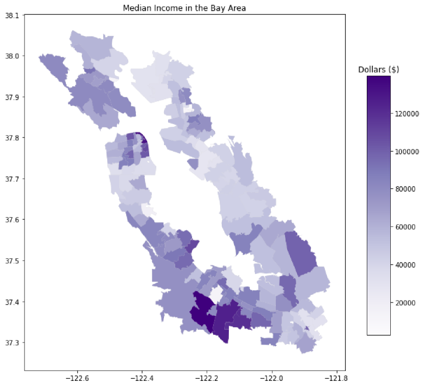
(a) Median income.

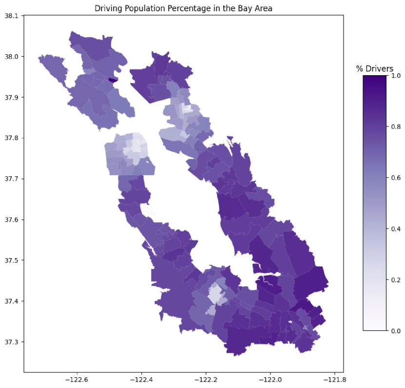
(b) Driving population percentage.

Figure 1: Driving population percentage and median income distribution in San Francisco Bay Area from ACS.

We model the freeway network in the San Francisco Bay Area as a network with 17 nodes (Figure 2). Each node represents a major work or home location for travelers, and the edges represent the primary freeways connecting these locations. Since willingness-to-pay is a latent parameter that cannot be directly estimated from the data, we use the median individual income as a proxy to categorize travelers with home at each node into three types of populations with low, middle and high willingness-to-pay, respectively. This is justified by the empirical evidence that the variations of willingness-to-pay are often associated with income levels (Athira et al.,, 2016; Gunn,, 2001; Waters,, 1994; Thomas and Thompson,, 1970). Using high-fidelity datasets from Safegraph, the Caltrans Performance Measurement System (PeMS), and the American Community Survey (ACS), we calibrate the latency function of each edge and the demand of each traveler population with each willingness-to-pay and each home-work node pair.

The current congestion pricing scheme, denoted as curr  sets $\$7$ price on each of the bridges in the Bay Area (Figure 2). We compute the four congestion pricing schemes (hom, het, hom_sc, het_sc), and compare the resulting equilibrium routing behavior in comparison to curr and the zeropricing scheme that set no tolls. We summarize our finding below:

• Efficiency: All four proposed pricing schemes leads to a lower congestion level compared to curr. Surprisingly, curr is also marginally outperformed by zero. This is primarily attributed to the fact that the homogeneous toll price of $7 on all bridges under curr does not account for the heterogeneous distribution of travelers with different home-work locations and different willingness-to-pay. We show that hom and het achieve the minimum congestion, as indicated by our theoretical result (Proposition 4.2). Additionally, hom_sc and het_sc achieve lower congestion level than curr and zero but higher than hom and het. Furthermore, we find that the price of anarchy (POA) – the ratio between the total travel time in equilibrium with no tolls and that of the minimum total travel time (Roughgarden,, 2010) – in our setup is 1.04, which is close to 1. This is likely due to high total demand of travelers in the Bay area network since POA always converges to 1 in routing games as the population demand increases (Colini-Baldeschi et al.,, 2020; Cominetti et al.,, 2021).

• Equity: We observe that all pricing schemes except for hom lead to lower travel cost for all traveler types in comparison to curr  (otherwise stated, these pricing schemes lead to Pareto improvements in travel cost). Furthermore, the percentage of travelers with travel costs exceeding a certain threshold is higher in homogeneous pricing schemes than in heterogeneous pricing schemes, irrespective of the population type and the specified threshold. This is due to the fact that heterogeneous pricing schemes adjust the toll prices according to the population’s willingness-to-pay, and thus resulting in lower monetary costs for travelers with low willingness-to-pay. Additionally, the proportion of travelers with costs above a certain threshold is lower in pricing schemes with support constraints, regardless of the type and the threshold. Such difference is more significant under homogeneous pricing schemes compared to heterogeneous ones.

• Revenue Generation: We observe that the revenue generated by hom is the highest as it charges high tolls to all travelers in order to achieve the minimum congestion. Moreover, the revenues generated by het, hom_sc and het_sc are comparable to curr  with het being marginally higher and, hom_sc and het_sc, marginally lower.

The rest of the paper is organized as follows: Section 2 presents an overview of past works related to our paper. Section 3 presents the model of routing games with heterogeneous populations. Section 4 presents the computation methods for the four congestion pricing schemes (hom, het, hom_sc, and het_sc). Section 5 presents calibration of the routing game model in the San Francisco Bay Area. Section 6 presents the efficiency and equity evaluation of the proposed pricing schemes and the comparison of the emerging congestion patterns.

2 Related works

The literature on designing congestion pricing schemes can be categorized into two main threads: first-best and second-best. First-best pricing schemes allow tolls to be placed on every edge of the network. The most popular first-best tolling scheme is marginal cost pricing, which sets the toll price to be the marginal cost created by an additional unit of congestion on each edge (Arnott and Small,, 1994; Beckmann et al.,, 1956; Smith,, 1979; Roughgarden,, 2010). Additionally, an extensive line of research in this thread also focuses on characterizing the set of all congestion-minimizing toll prices (Bergendorff et al.,, 1997; Hearn and Ramana,, 1998; Dial,, 2000; Yildirim and Hearn,, 2005; Fleischer et al.,, 2004; Bai et al.,, 2004; Cole et al.,, 2003; Karakostas and Kolliopoulos,, 2004; Yang and Huang,, 2004). On the other hand, second-best pricing schemes restrict the set of edges that can be tolled. The literature on second-best pricing schemes primarily focuses on formulating the problem as a mathematical program with equilibrium constraints (MPEC) and developing algorithms to approximate the optimal solution (Yang and Lam,, 1996; Brotcorne et al.,, 2001; Ferrari,, 2002; Labbé et al.,, 1998; Larsson and Patriksson,, 1998; Lim,, 2002; Patriksson and Rockafellar,, 2002; Verhoef,, 2002; Lawphongpanich and Hearn,, 2004; Ekström et al.,, 2009; Kalashnikov et al.,, 2016). Some works have also considered a complementary problem of finding the minimum number of toll booths required to ensure the efficient allocation of traffic (Bai et al.,, 2010; Bai and Rubin,, 2009). Moreover, (Hoefer et al.,, 2008; Bonifaci et al.,, 2011; Harks et al.,, 2015) studied the problem of characterizing the hardness of the problem of designing second-best tolls. The paper (Hoefer et al.,, 2008) showed that it is NP hard to compute optimal tolls on a subset of edges in general networks and gave a polynomial time algorithm to solve the problem for the parallel link case with affine latency functions. This was extended to allow for non-affine latency functions by (Harks et al.,, 2015), and upper bound on the toll values in (Bonifaci et al.,, 2011). From a computational perspective, (Harks et al.,, 2015) proposed a gradient based heuristic algorithm that iteratively computes the Wardrop equilibrium in each round of the algorithm to descend along the gradient of the objective function. In our setup, hom and het are first-best pricing schemes and hom_sc and het_sc are second-best pricing schemes. We contribute to this line of literature by proposing a multi-step linear programming based approach to compute hom and het that account for the equity objective and the heterogeneous traveler populations. Our approach is also an efficient heuristic to solve hom_sc and het_sc with atmost three linear programs instead of iteratively computing the Wardrop equilibrium.

The literature on congestion pricing has mostly focused on homogeneous pricing schemes with a few exceptions. The paper (Feng et al.,, 2023) considered tolling schemes that differentiate conventional vehicles from clean energy vehicles. Moreover, differentiated tolls are also used in (Lazar and Pedarsani,, 2021, 2020; Mehr and Horowitz,, 2019) for the study of mixed autonomy. The paper (Brown and Marden,, 2016) studied the impact of differentiated tolling in parallel-link networks with affine cost functions and travelers that have heterogeneous value of time.

One effort to ameliorate the inequities resulting from congestion pricing is to refund (a fraction of) toll revenue to a subset of traveler populations. The papers (Goodwin,, 1990; Small,, 1992) were amongst the first to propose different ways to redistribute the revenue in form of infrastructure development and tax rebates. The effectiveness of redistribution schemes are theoretically analyzed in single-lane bottleneck models ((Arnott and Small,, 1994; Bernstein,, 1993)), parallel networks ((Adler and Cetin,, 2001)), and single origin-destination network ((Eliasson,, 2001)).

Pareto-improving congestion pricing schemes were introduced as another approach to reduce inequality. First proposed by (Lawphongpanich and Yin,, 2007), Pareto-improving congestion pricing minimizes the total congestion while ensuring that no travelers are worse off in comparison to no tolls. The paper (Song et al.,, 2009) studied the design of Pareto-improving schemes for travelers with heterogeneous willingness-to-pay, and (Lawphongpanich and Yin,, 2010) further proved that such Pareto-improving schemes only exist in special classes of networks. The paper (Guo and Yang,, 2010) studied the problem of designing Pareto-improving pricing schemes combined with revenue refund. (Jalota et al.,, 2021) extended this line of research by developing optimal revenue refunding schemes to minimize the congestion and inequity together. In both (Guo and Yang,, 2010) and (Jalota et al.,, 2021), the tolls minimize the weighted sum of total travel time with weights being each population’s value of time. This objective is different from our goal of minimizing the actual congestion level (unweighted total travel time), which is a more suitable metric to assess the environmental impact of congestion.

The third approach to addressing inequality is the study of fairness constrained traffic assignment problem proposed by (Jahn et al.,, 2005), where the fairness metric is the maximum difference of travel time experienced by travelers between the same origin-destination pair. (Angelelli et al.,, 2016, 2021) extended this line of research by developing algorithmic methods to solve the fairness constrained traffic assignment problem. The problem of devising congestion pricing schemes which could enforce the resulting traffic assignment patters was studied in (Jalota et al.,, 2023). Particularly, (Jalota et al.,, 2023) studies homogeneous pricing scheme that implements the traffic assignment minimizing an interpolation of the potential function (which is used to characterize the equilibrium) and the social cost function.

Our work contributes to all of the above studies on the equity of congestion pricing from three aspects: (i) Our equity consideration accounts for both the travel time cost and the monetary cost that includes both the toll and the gas prices. This generalizes the fairness notion that focuses only on the travel time difference; (ii) Our tolling scheme minimizes the total congestion in the network (i.e. guarantees the optimal efficiency) while provides the central planner a flexible way to trade-off between the total welfare, equity across heterogeneous populations and total revenue. In particular, by tuning the parameter that governs the trade-off between the average welfare and equity, we can increase or reduce the revenue collected by the our pricing scheme; (iii) We provide a comprehensive evaluation of different congestion pricing schemes in terms of efficiency, equity and revenue using real-world data collected in the San Francisco Bay Area.

Finally, on the empirical side, (Frick et al.,, 1996; Nakamura and Kockelman,, 2002; Barnes et al.,, 2012; Zhang et al.,, 2011) focused on understanding the impact of congestion pricing of the San Francisco-Oakland Bay Bridge, which is the most heavily congested segment in the San Francisco Bay Area highway network. Particularly, (Frick et al.,, 1996) initiated the study to employ congestion pricing schemes to alleviate congestion on the Bay Bridge. (Nakamura and Kockelman,, 2002) studied the problem of combining tolls with road rationing protocols to reduce congestion on the Bay Bridge. (Zhang et al.,, 2011; Barnes et al.,, 2012) studied the reduction in travel time of different type of travelers (such as FasTrak travelers, cash customers and HOV travelers) after the implementation of a new congestion pricing scheme on the bridge in 2010. Our work generalizes this line of work to the entire Bay Area highway network using high-fidelity mobility and socioeconomic datasets.

3 Model

In this section, we introduce the non-atomic networked routing game model that forms the basis for our theoretical and computational results. We introduce equilibrium routing and the four types of congestion pricing schemes we consider in this paper.

3.1 Network

Consider a transportation network $G=(N,E)$, where $N$ is the set of nodes, and $E$ is the set of edges. A set of non-atomic travelers (agents) make routing decisions in the network between their origin and destination. We denote the set of origin-destination (o-d) pairs as $K$ and the set of routes (i.e. sequences of edges) connecting each o-d pair $k\in K$ as $R^{k}$.

Travelers for each o-d pair $k$ are grouped into $I$ populations, where each population is associated with a different level of willingness-to-pay $\theta^{i}\in\mathbb{R}_{\geq 0}$ that represents the amount of money that agents in population $i$ are willing to pay to save a unit of travel time cost. We refer to agents with willingness-to-pay $\theta^{i}$ as type $i$ agents. The demand vector is given by $D=(D^{ik})_{i\in I,k\in K}$, where $D^{ik}$ is the demand of agents with type $i$ that want to travel between o-d pair $k$. Throughout this paper, we operate under the inelastic demand assumption: traveler demands on each origin-destination pair are constant. This assumption is reasonable given that (a) our analysis focuses on the commuting behavior during the morning rush hour, when the majority of trips are work-related with little elasticity; (b) the availability of public transit is sparse and the cost of car ownership is high (Depillis et al.,, 2023).

The strategy distribution of agents is denoted $q=(q^{ik}_{r})_{r\in R^{k},i\in I,k\in K}$ , where $q^{ik}_{r}$ is the flow of agents with type $i$ and o-d pair $k$ who take route $r$. Therefore, the set of feasible strategy distributions is given by:

$$\mathcal{Q}(D):=\left\{q=(q_{r}^{ik}):\sum_{r\in R^{k}}q_{r}^{ik}=D^{ik},\quad q_{r}^{ik}\geq 0\quad\forall r\in R^{k},i\in I,k\in K\right\}.$$ (1)

Given a strategy distribution $q\in\mathcal{Q}(D)$, the flow of agents of type $i\in I$ on edge $e\in E$ is given by

$$f_{e}^{i}(q):=\sum_{k\in K}\sum_{r\in R^{k}}q_{r}^{ik}\mathbbm{1}(e\in r),$$ (2)

and the total flow of agents on edge $e\in E$ is

$$w_{e}(q):=\sum_{i\in I}f_{e}^{i}(q).$$ (3)

The travel time experienced by agents taking edge $e\in E$ is $\ell_{e}(w_{e}(q))$, where the latency function $\ell_{e}\colon\mathbb{R}_{+}\to\mathbb{R}_{+}$ is continuous, strictly increasing, and convex. Consequently, the total travel time experienced by agents from o-d pair $k\in K$ who use route $r\in R^{k}$ is given by $\ell_{r}(q):=\sum_{e\in r}\ell_{e}(w_{e}(q)).$ With slight abuse of notation, we use $\ell_{r}(q)$ and $\ell_{r}(w)$ interchangeably to represent the latency of route $r$ where $w$ is the edge flow vector corresponding to the strategy distribution $q$. In addition to the travel time, the total cost experienced by each individual agent also includes the congestion price imposed by the planner, and the gas cost required to travel on the route the agent chooses. In particular, let $p_{e}^{i}$ be the toll price imposed on travelers of type $i\in I$ for using edge $e\in E$, and $g_{e}$ be the gas cost of using an edge $e\in E$. Note that we allow for the toll price to be type-specific in the general setting. We will later discuss different scenarios for setting the toll prices. Given the tolls $p=(p_{e}^{i})_{e\in E,i\in I}$, the cost experienced by travelers of type $i\in I$ associate with o-d pair $k\in K$ and taking route $r\in R^{k}$ is given by

$$c_{r}^{i}(q,p):=\ell_{r}(q)+\frac{1}{\theta^{i}}\sum_{e\in r}(p_{e}^{i}+g_{e}).$$ (4)

Crucially, a key feature of our model is that the toll and gas costs experienced by each agent are modulated by the willingness-to-pay $\theta^{i}$ of that agent. This allows us to model the heterogeneity present in the types of travelers. Given this setup, we define Nash equilibrium to be the strategy distribution such that no traveler has incentive to deviate from their chosen route. That is,

Definition 3.1.

For any tolls $p$, a strategy profile $q^{*}(p)$ is a Nash equilibrium if

$$\forall i\in I,k\in K,r\in R^{k},\quad q_{r}^{ik*}(p)>0\quad\Rightarrow\quad c_{r}^{i}(q^{*}(p),p)\leq c_{r^{\prime}}^{i}(q^{*}(p),p)\ \quad\forall r^{\prime}\in R^{k}.$$

The objective of the planner is to minimize the network congestion, measured by the total travel time cost experienced by all travelers. For any strategy distribution $q$, we denote the planner’s cost function as follows:

$$S(q):=\quad \sum_{e\in E}w_{e}(q)\ell_{e}(w_{e}(q)),$$ (5)

where $w_{e}(q)$ is given by (3). We denote the set of socially optimal strategy distributions as $q^{\dagger}:=\operatorname*{arg\,min}_{q\in\mathcal{Q}(D)}S(q)$, and the induced socially optimal edge flows as $w^{\dagger}=(w^{\dagger}_{e})_{e\in E}$, where $w^{\dagger}_{e}=w_{e}(q^{\dagger})$ given by (3).

3.2 Congestion pricing

We now introduce two practical considerations for toll implementation. The first consideration is whether or not the toll is type-specific. In particular, a congestion pricing scheme is homogeneous if the toll is uniform across all population types, and heterogeneous if the toll varies with population types (formally, whether $p_{e}^{i}$ is allowed to depend on $i$ or not, on each edge). The challenge of implementing a heterogeneous scheme is that the willingness-to-pay is a latent variable that is privately known only by the individual traveler. In practice, an individual’s willingness-to-pay is often closely correlated with their income level, i.e. higher-income groups are typically associated with a higher willingness-to-pay, while lower-income groups correlate with a lower willingness-to-pay (Athira et al.,, 2016; Gunn,, 2001; Waters,, 1994; Thomas and Thompson,, 1970). Therefore, one way to implement heterogeneous tolling is to set tolls based on the income level of travelers. For example, low income groups, which have significant overlap with the population of low willingness-to-pay travelers, may receive a subsidy or a toll rebate in certain areas. Such toll relief programs have been established in several states in the United States, e.g. California , Virginia , New York etc.

The second consideration is whether or not tolls can be set on all the edges of the network or only on a subset (formally, whether or not $p_{e}^{i}$ is allowed to be strictly positive on all $e\in E$). In practical terms, congestion pricing often requires the installation of infrastructure facilities, which might not be feasible on all road segments. Thus, a congestion pricing scheme has no support constraints if tolls can be imposed on all edges, or has support constraints if tolls can only be imposed on a subset of edges, denoted as $E_{T}$. We note that congestion pricing schemes with (resp. without) support constraints are also referred as first-best (resp. second-best) tolling schemes in literature.

Building on the above two considerations, we define four types of tolling schemes:

• Homogeneous tolls with no support constraints (hom): $p_{e}^{i}\geq 0$ and $p_{e}^{i}=p_{e}^{j}$ for all $e\in E$ and all $i,j\in I$;

• Heterogeneous tolls with no support constraints (het): $p_{e}^{i}\geq 0$ for all $e\in E,i\in I$;

• Homogeneous tolls with support constraints (hom_sc): $p_{e}^{i}=p_{e}^{j}$ for all $i,j\in I$ and all $e\in E$. Additionally, $p_{e}^{i}=0$ for all $e\in E\backslash E_{T}$, and $p_{e}^{i}\geq 0$ for all $e\in E_{T}$.

• Heterogeneous tolls with support constraints (het_sc): $p_{e}^{i}=0$ for all $e\in E\backslash E_{T}$, and $p_{e}^{i}\geq 0$ for all $e\in E_{T}$.

4 Computation methods

In this section, we outline methods for computing equilibrium routing strategies and the four congestion pricing schemes. We first establish that, given any fixed toll values, the equilibrium outcome can be derived as the optimal solution to a convex optimization problem. We then demonstrate that the set of homogeneous tolls (hom) and heterogeneous tolls (het) without support constraints that realize the socially optimal edge flows can be characterized as the set of optimal solutions of linear programs. Next, we present a multi-step approach for calculating the toll prices that strikes a balance between equity, as measured by the cost disparity between travelers from different populations, and at the same time, maximizing the welfare of all traveler populations. For congestion pricing schemes with support constraints, we adapt our approach to provide a heuristic for calculating hom_sc and het_sc, acknowledging that such solutions may not guarantee the implementation of the socially optimal edge flows.

Proposition 4.1.

Given toll prices $p$, a strategy distribution $q^{\ast}(p)$ is a Nash equilibrium if and only if it is a solution to the following convex optimization problem:

$$\min_{q\in\mathcal{Q}(D)}\quad \Phi(q,p,\theta)=\sum_{e\in E}\int_{0}^{w_{e}(q)}\ell_{e}(z)\ \mathrm{d}z+\sum_{i\in I}\sum_{e\in E}\frac{(p_{e}^{i}+g_{e})}{\theta^{i}}f_{e}^{i}(q),$$ (6)

where $w_{e}^{i}(q)$, $w_{e}(q)$ are given by (2) and (3), respectively. Moreover, given any toll price vector $p$, the equilibrium edge flow vector $w^{*}(p):=w(q^{*}(p))$ is unique. Additionally, the socially optimal edge flow vector $w^{\dagger}$ is unique.

Proposition 4.1 is an extension of (Guo and Yang,, 2010) to incorporate the gas price in the cost function for each population. The proof of this result builds on the fact that (a) the equilibrium condition in the routing game is equivalent to the optimality condition of the convex program (6), and (b) (6) is strictly convex in the edge load vector $w$. To make the paper self-contained, we include the proof in Appendix A.

Proposition 4.1 shows that the socially optimal edge load vector $w^{\dagger}$ is unique. However, we note that such a $w^{\dagger}$ may be induced by multiple type-specific flow vectors $f^{\dagger}$. Although these different type-specific flow vectors all induce the same aggregate edge load, and thus minimize the total cost, they may lead to different travel time costs experienced by different population types.

Next, we show that the set of prices hom (resp. het) that implements the socially optimal edge load can be characterized each by a linear program.

Proposition 4.2.

• A homogeneous congestion pricing scheme $p^{\dagger}=(p^{\dagger}_{e})_{e\in E}$ implements the socially optimal edge flow $w^{\dagger}=(w^{\dagger}_{e})_{e\in E}$ if and only if there exists $z^{\dagger}$ such that $(p^{\dagger},z^{\dagger})$ is a solution to the following linear program:

  $$T^{\ast}_{\textsf{hom}}=\max_{p,z} ~{}\sum_{i\in I}\sum_{k\in K}D^{ik}z^{ik}-\sum_{e\in E}p_{e}w_{e}^{\dagger}, \mathcal{P}_{\textsf{hom}}$$ ()

  s.t. $$~{}z^{ik}-\sum_{e\in r}(p_{e}+g_{e})\leq\theta^{i}\ell_{r}(w^{\dagger}),\quad\forall k\in K,r\in R^{k},i\in I,$$

  $$~{}p_{e}\geq 0,\quad\forall e\in E.$$

• A heterogeneous congestion pricing scheme $p^{\dagger}=(p^{i\dagger}_{e})_{e\in E,i\in I}$ implements a type-specific socially optimal edge flow $f^{\dagger}=(f_{e}^{i})_{e\in E,i\in I}$ if and only if there exists a $z^{\dagger}$ such that $(p^{\dagger},z^{\dagger})$ is a solution to the following linear program:

  $$T^{\ast}_{\textsf{het}}(f^{\dagger})=\max_{p,z} ~{}\sum_{i\in I}\sum_{k\in K}D^{ik}z^{ik}-\sum_{e\in E}\sum_{i\in I}p_{e}^{i}f_{e}^{\dagger i}, \mathcal{P}_{\textsf{het}}$$ ()

  s.t. $$~{}z^{ik}-\sum_{e\in r}(p_{e}^{i}+g_{e})\leq\theta^{i}\ell_{r}(w^{\dagger}),\quad\forall k\in K,r\in R^{k},i\in I,$$

  $$~{}p_{e}^{i}\geq 0,\quad\forall e\in E,i\in I.$$

Proposition 4.2 builds on a result in (Fleischer et al.,, 2004). In particular, (Fleischer et al.,, 2004) showed that any optimal solution of ($\mathcal{P}_{\textsf{hom}}$) is a congestion minimizing toll price vector in hom. We show that the other direction of this argument also holds: any congestion minimizing toll price vector in hom must be an optimal solution of ($\mathcal{P}_{\textsf{hom}}$). Additionally, we extend the result of hom to het to show that a heterogeneous toll price vector induces the a congestion minimizing flow if and only if it is an optimal solution of ($\mathcal{P}_{\textsf{het}}$).

The proof of Proposition 4.2 builds on the two linear programs ($\mathcal{P}_{\textsf{hom}}$) – ($\mathcal{P}_{\textsf{het}}$) and their dual programs ($\mathcal{D}_{\textsf{hom}}$) and ($\mathcal{D}_{\textsf{het}}$) as follows:

$$\min_{q} ~{}~{}\sum_{i\in I}\sum_{k\in K}\sum_{r\in R^{k}}(\theta^{i}\ell_{r}(w^{\dagger})+\sum_{e\in r}g_{e})q_{r}^{ik} \mathcal{D}_{\textsf{hom}}$$ ()

s.t. $$~{}~{}\sum_{i\in I}\sum_{k\in K}\sum_{r\in R^{k}:e\in r}q_{r}^{ik}\leq w_{e}^{\dagger},\quad\forall e\in E, \mathcal{D}_{\textsf{hom}.a}$$ ()

$$~{}~{}\sum_{r\in R^{k}}q_{r}^{ik}=D^{ik},\quad\forall i\in I,k\in K, \mathcal{D}_{\textsf{hom}.b}$$ ()

$$~{}~{}q_{r}^{ik}\geq 0\quad\forall i\in I,k\in K,r\in R^{k}. \mathcal{D}_{\textsf{hom}.c}$$ ()

$$\min_{q} ~{}~{}\sum_{i\in I}\sum_{k\in K}\sum_{r\in R^{k}}(\theta^{i}\ell_{r}(w^{\dagger})+\sum_{e\in r}g_{e})q_{r}^{ik} \mathcal{D}_{\textsf{het}}$$ ()

s.t. $$~{}~{}\sum_{k\in K}\sum_{r\in R^{k}:e\in r}q_{r}^{ik}\leq f_{e}^{\dagger i},\quad\forall e\in E,i\in I, \mathcal{D}_{\textsf{het}.a}$$ ()

$$~{}~{}\sum_{r\in R^{k}}q_{r}^{ik}=D^{ik},\quad\forall i\in I,k\in K, \mathcal{D}_{\textsf{het}.b}$$ ()

$$~{}~{}q_{r}^{ik}\geq 0,\quad\forall i\in I,k\in K,r\in R^{k}. \mathcal{D}_{\textsf{het}.c}$$ ()

In our proof, we show that under both hom and het, the feasibility constraints of the associated primal and dual programs as well as the complementary slackness conditions are equivalent to the equilibrium condition where only routes with the minimum cost are taken by travelers. Moreover, we show that constraints ($\mathcal{D}_{\textsf{hom}.a}$) and ($\mathcal{D}_{\textsf{het}.a}$) must be tight at optimality, indicating that the induced flow vector in equilibrium is indeed the congestion minimizing flow vector. Therefore, the set of optimal solutions of ($\mathcal{P}_{\textsf{hom}}$) and ($\mathcal{P}_{\textsf{het}}$) are the set of toll vectors that induce the congestion minimizing flow under hom and het, respectively.

We denote $P^{\dagger}_{\hom}$ as the set of socially optimal toll prices for hom, and $P^{\dagger}_{\textsf{het}}(f^{\dagger})$ as the set of socially optimal toll price for het that induces a type-specific socially optimal edge flow $f^{\dagger}$. Proposition 4.2 demonstrates that both sets can be computed as the optimal solution set of linear programs. In particular, we note that the set $P^{\dagger}_{\textsf{het}}(f^{\dagger})$ depends on which edge-specific socially optimal flow $f^{\dagger}$ is induced since the objective function ($\mathcal{P}_{\textsf{het}}$) depends on $f^{\dagger}$.

Furthermore, $P^{\dagger}_{\hom}$ and $P^{\dagger}_{\textsf{het}}(f^{\dagger})$ may not be singleton sets. This presents a challenge for the planner, who must then decide which specific toll price from the optimal solution set to implement. While all tolls in $P^{\dagger}_{\hom}$ and $P^{\dagger}_{\textsf{het}}$ achieve the minimum social cost, they do so by impacting travelers differently given their individual origin-destination pair and willingness-to-pay. We consider that the central planner aims at solving the following problem:

$$\begin{split}\min_{p}~{}&L(p):=\underbrace{\max_{i,i^{\prime}\in I}\bigg{|}\frac{1}{D^{i}}\sum_{k\in K}D^{ik}c^{ik\dagger}(p)-\frac{1}{D^{i^{\prime}}}\sum_{k\in K}D^{i^{\prime}k}c^{i^{\prime}k\dagger}(p)\bigg{|}}_{(i)}+\lambda\underbrace{\frac{1}{D}\sum_{i\in I}\sum_{k\in K}D^{ik}c^{ik\dagger}(p)}_{(ii)},\\ s.t.\quad\quad&p\in\left\{\begin{array}[]{ll}P^{\dagger}_{\hom},&\quad\text{in $\textsf{hom}$,}\\ P^{\dagger}_{\textsf{het}}(f^{\dagger}),&\quad\text{in $\textsf{het}$ with the population-specific optimal flow $f^{\dagger}$.}\end{array}\right.\end{split}$$ (8)

where $D^{i}=\sum_{k\in K}D^{ik}$ and $D=\sum_{i\in I}D^{i}$, $\lambda\geq 0$ and

$$c^{ik\dagger}(p)=\min_{r\in R^{k}}\left\{\ell_{r}(w^{\dagger})+\frac{1}{\theta^{i}}\sum_{e\in r}(p_{e}+g_{e})\right\}$$ (9)

is the equilibrium cost of individuals with o-d pair $k$ and type $i$ given the toll price $p$ and socially optimal edge load $w^{\dagger}$.

In (8), (i) can be viewed as an equity metric that evaluates the maximum difference of average equilibrium cost of travelers with each type and (ii) is an average welfare metric that is the average travel time experienced by all travelers. We emphasize that the cost $c^{ik\dagger}(p)$ as in (9) is the minimum cost of choosing a route given the socially optimal load vector $w^{\dagger}$, the toll price and the gas fee. This is indeed an equilibrium cost of traveler population with type $i$ and o-d pair $k$ since any $p\in P^{\dagger}_{\hom}$ or $p\in P^{\dagger}_{\textsf{het}}(f^{\dagger})$ guarantees that the equilibrium edge vector is $w^{\dagger}$. The objective function in (8) indicates that the central planner selects the congestion minimizing toll price that also balances the equity among populations with different willingness-to-pay and the average welfare that accounted for the travel time cost as well as the toll price and gas fee. Balancing welfare maximization with cost disparity minimization avoids the potential problem with just minimizing cost disparity: charging excessively high tolls to every type of travelers. In (8), $\lambda\geq 0$ is the parameter that governs the relative weight between the equity objective and the welfare objective.

We denote the socially optimal homogeneous congestion pricing scheme that solves the central planner’s problem (8) as $p^{*}_{\hom}$. The next proposition shows that we can solve the central planner’s problem (8) for hom by another linear program.

Proposition 4.3.

For the $\hom$ tolling scheme, $p^{*}_{\hom}$ is an optimal solution of the following linear program:

$$\min_{p,z,y} y+\frac{\lambda}{D}\sum_{i\in I}\sum_{k\in K}D^{ik}z^{ik} \mathcal{P}^{\ast}_{\textsf{hom}}$$ ()

s.t. $$y\geq\frac{1}{D^{i}}\sum_{k\in K}\frac{D^{ik}z^{ik}}{\theta^{i}}-\frac{1}{D^{i^{\prime}}}\sum_{k\in K}\frac{D^{i^{\prime}k}z^{i^{\prime}k}}{\theta^{i}}, \forall i,i^{\prime}\in I, \mathcal{P}^{\ast}_{\textsf{hom}.a}$$ ()

$$\sum_{i\in I}\sum_{k\in K}D^{ik}z^{ik}-\sum_{e\in E}p_{e}w_{e}^{\dagger}\geq T^{\ast}_{\textsf{hom}}, \mathcal{P}^{\ast}_{\textsf{hom}.b}$$ ()

$$z^{ik}-\sum_{e\in r}(p_{e}+g_{e})\leq{\theta^{i}}\ell_{r}(w^{\dagger}), \forall k\in K,r\in R^{k},i\in I, \mathcal{P}^{\ast}_{\textsf{hom}.c}$$ ()

$$p_{e}\geq 0 \forall e\in E, \mathcal{P}^{\ast}_{\textsf{hom}.d}$$ ()

where $T^{\ast}_{\textsf{hom}}$ is the optimal value of the objective function. of($\mathcal{P}_{\textsf{hom}}$).

In ($\mathcal{P}^{\ast}_{\textsf{hom}}$), constraints ($\mathcal{P}^{\ast}_{\textsf{hom}.c}$) and ($\mathcal{P}^{\ast}_{\textsf{hom}.d}$) ensure that variables $(p,z)$ are in the feasible set of ($\mathcal{P}_{\textsf{hom}}$), and constraint ($\mathcal{P}^{\ast}_{\textsf{hom}.b}$) further restrict that the set of $(p,z)$ in ($\mathcal{P}^{\ast}_{\textsf{hom}}$) to be the set of optimal solutions of ($\mathcal{P}_{\textsf{hom}}$). Thus, following Proposition 4.2, any feasible $p$ in ($\mathcal{P}^{\ast}_{\textsf{hom}}$) must be a toll vector that induces the socially optimal edge flow $w^{\dagger}$. Moreover, the proof of Proposition 4.2 further ensures that for every $i\in I,k\in K$ there exists $r\in R^{k}$ such that the corresponding constraint in ($\mathcal{P}^{\ast}_{\textsf{hom}.c}$) must be tight at optimum, which indicates that any $z^{ik}$ in ($\mathcal{P}^{\ast}_{\textsf{hom}}$) equals to $\theta^{i}\cdot c^{ik\dagger}(p)$. Additionally, constraints ($\mathcal{P}^{\ast}_{\textsf{hom}.a}$) guarantee that at optimality $y=\max_{i,i^{\prime}\in I}\bigg{|}\frac{1}{D^{i}}\sum_{k\in K}D^{ik}c^{ik\dagger}(p)-\frac{1}{D^{i^{\prime}}}\sum_{k\in K}D^{i^{\prime}k}c^{i^{\prime}k\dagger}(p)\bigg{|}$. Thus, the linear program ($\mathcal{P}^{\ast}_{\textsf{hom}}$) computes the congestion minimizing $\hom$ toll price that optimizes the equity and welfare objectives with relative weight $\lambda$.

Propositions 4.2 and 4.3 provide a two-step approach of computing $p^{*}_{\hom}$: first, compute $T^{\ast}_{\textsf{hom}}$ by solving the linear program ($\mathcal{P}_{\textsf{hom}}$) given the unique congestion minimizing edge flow $w^{\dagger}$. Second, compute $p^{*}_{\hom}$ by solving the linear program ($\mathcal{P}^{\ast}_{\textsf{hom}}$) using $T^{\ast}_{\textsf{hom}}$.

Next, we show that the central planner can compute the congestion minimizing toll price vector for het that optimizes the equity-welfare objective function (8), denoted as $p^{*}_{\textsf{het}}$, using a similar approach as described above. However, in het, one additional issue arises as both the congestion minimizing toll price set $P^{\dagger}_{\textsf{het}}(f^{\dagger})$ and consequently $p^{*}_{\textsf{het}}$ depend on the selection of the type-specific flow vector $f^{\dagger}$, which is not unique. Here, we propose to select the congestion minimizing population-specific flow vector $f^{\dagger}$ as the one that induces the congestion minimizing flow vector $w^{\dagger}$ while also minimizing the difference of average travel time cost across all traveler populations. To compute such a $f^{\dagger}$, we first find a feasible routing strategy profile $q^{\dagger}$ that induces $w^{\dagger}$ and minimizes the average cost difference among traveler populations. Such a $q^{\dagger}$ can be solved by the following linear program:

$$\min_{q} x,$$ (11)

s.t. $$x\geq\sum_{k\in K}\sum_{r\in R^{k}}q_{r}^{ik}\ell_{r}(w^{\dagger})-\sum_{k\in K}\sum_{r\in R^{k}}q_{r}^{i^{\prime}k}\ell_{r}(w^{\dagger}), \forall i,i^{\prime}\in I,$$

$$\sum_{r\in R^{k}}q_{r}^{ik}=D^{ik}, \forall\ i\in I,k\in K,$$

$$\sum_{i\in I}\sum_{k\in K}\sum_{r\in R^{k}:e\in r}q_{r}^{ik}=w^{\dagger}_{e}, \forall e\in E,$$

$$q_{r}^{ik}\geq 0, \forall\ i\in I,k\in K,r\in R^{k}.$$

Then, the induced population-specific flow vector $f^{\dagger}$ associated with $q^{\dagger}$ is given by (2). Based on $f^{\dagger}$, we compute $p^{*}_{\textsf{het}}$ as the optimal solution of a linear program.

Proposition 4.4.

For the het tolling scheme, given $f^{\dagger}$, $p^{*}_{\textsf{het}}$ is an optimal solution of the following linear program:

$$\min_{p,z,y} y+\frac{\lambda}{D}\sum_{i\in I}\sum_{k\in K}D^{ik}z^{ik} \mathcal{P}^{\ast}_{\textsf{het}}$$ ()

s.t. $$y\geq\frac{1}{D^{i}}\sum_{k\in K}\frac{D^{ik}z^{ik}}{\theta^{i}}-\frac{1}{D^{i^{\prime}}}\sum_{k\in K}\frac{D^{i^{\prime}k}z^{i^{\prime}k}}{\theta^{i}}, \forall i,i^{\prime}\in I, \mathcal{P}^{\ast}_{\textsf{het}.a}$$ ()

$$\sum_{i\in I}\sum_{k\in K}D^{ik}z^{ik}-\sum_{e\in E}p_{e}w_{e}^{\dagger}\geq T^{\ast}_{\textsf{het}}(f^{\dagger}), \mathcal{P}^{\ast}_{\textsf{het}.b}$$ ()

$$z^{ik}-\sum_{e\in r}(p_{e}^{i}+g_{e})\leq{\theta^{i}}\ell_{r}(w^{\dagger}), \forall k\in K,r\in R^{k},i\in I, \mathcal{P}^{\ast}_{\textsf{het}.c}$$ ()

$$p_{e}^{i}\geq 0, \forall e\in E, \mathcal{P}^{\ast}_{\textsf{het}.d}$$ ()

where $T^{\ast}_{\textsf{het}}(f^{\dagger})$ is the optimal value of the objective function of ($\mathcal{P}_{\textsf{het}}$) associated with $f^{\dagger}$.

Propositions 4.2 and 4.4 show that $p^{*}_{\textsf{het}}$ can be computed using a three-step approach: first, we compute the type-specific flow vector $f^{\dagger}$ that induces the congestion minimizing edge flow $w^{\dagger}$ while also minimizing the average cost difference among all traveler populations using (11). Second, we compute $T^{\ast}_{\textsf{het}}(f^{\dagger})$ using ($\mathcal{P}_{\textsf{het}}$) given $f^{\dagger}$. Third, we compute $p^{*}_{\textsf{het}}$ using ($\mathcal{P}^{\ast}_{\textsf{het}}$).

Finally, we discuss how to extend our approaches of computing $p^{*}_{\hom}$ and $p^{*}_{\textsf{het}}$ to incorporate the support constraints of the toll price. Previous studies (Hoefer et al.,, 2008; Bonifaci et al.,, 2011) showed that the problem of computing the congestion minimizing toll price with support set constraints is NP hard even without considering heterogeneous willingness-to-pay of travelers or equity objectives. Here, we provide heuristics for computing the toll prices with support constraints. We evaluate the performance of our heuristics in terms of congestion minimizing gap, equity, and welfare on the San Francisco Bay Area network in Sec. 4.

Heuristics for computing $p^{*}_{\textsf{hom\_sc}}$.

We propose a two-step heuristic to compute hom_sc by appropriately modifying the two-step method to compute hom.

We first solve the following linear program that adds the support constraints to ($\mathcal{P}_{\textsf{hom}}$):

$$T^{\ast}_{\textsf{hom\_sc}}=\max_{p,z} ~{}\sum_{i\in I}\sum_{k\in K}D^{ik}z^{ik}-\sum_{e\in E}p_{e}w_{e}^{\dagger}, \mathcal{P}_{\textsf{{hom\_sc}}}$$ ()

s.t. $$~{}z^{ik}-\sum_{e\in r}(p_{e}+g_{e})\leq\theta^{i}\ell_{r}(w^{\dagger}),\quad\forall k\in K,r\in R^{k},i\in I,$$

$$~{}p_{e}\geq 0,\quad\forall e\in E_{T},\quad p_{e}=0,\quad\forall e\in E\setminus E_{T}.$$

We note that the equilibrium edge load associated with any optimal solution of ($\mathcal{P}_{\textsf{{hom\_sc}}}$), say $\hat{w}$, may not be equal to the socially optimal edge load $w^{\dagger}$. This is because the constraints that edges in $E\setminus E_{T}$ having zero tolls remove the dual constraints in ($\mathcal{D}_{\textsf{hom}.a}$) for edges in $E_{T}$. As a result, the primal and dual argument in the proof of Proposition 4.2 no longer holds, and thus the induced edge flow $\hat{w}$ may not be equal to $w^{\dagger}$.

Note that the optimal solution to ($\mathcal{P}_{\textsf{{hom\_sc}}}$) will be non-unique. Therefore, inspired by ($\mathcal{P}^{\ast}_{\textsf{hom}}$), we consider the following heuristic to incorporate both equity and welfare metric while also accounting for support constraints. Note that simply adding the support constraints in ($\mathcal{P}^{\ast}_{\textsf{hom}}$) could render the optimization problem infeasible as the optimal set of homogeneous tolls $P^{\ast}_{\textsf{hom}}$ need not have a solution that satisfies the support constraints. Particularly the constraint ($\mathcal{P}^{\ast}_{\textsf{hom}.b}$) would get violated. This is because $T^{\ast}_{\textsf{hom}}\geq T^{\ast}_{\textsf{hom\_sc}}$ as the constraint set of ($\mathcal{P}^{\ast}_{\textsf{hom\_sc}}$) is contained in that of ($\mathcal{P}^{\ast}_{\textsf{hom}}$). Therefore, we compute $p^{*}_{\textsf{hom\_sc}}$ as the optimal solution of the following linear program which adds support constraints to ($\mathcal{P}^{\ast}_{\textsf{hom}}$) while relaxing the constraint ($\mathcal{P}^{\ast}_{\textsf{hom}.b}$) by using $T^{\ast}_{\textsf{hom\_sc}}$ instead of $T^{\ast}_{\textsf{hom}}$:

$$\min_{p,z,y} y+\frac{\lambda}{D}\sum_{i\in I}\sum_{k\in K}D^{ik}z^{ik} \mathcal{P}^{\ast}_{\textsf{hom\_sc}}$$ ()

s.t. $$y\geq\frac{1}{D^{i}}\sum_{k\in K}\frac{D^{ik}z^{ik}}{\theta^{i}}-\frac{1}{D^{i^{\prime}}}\sum_{k\in K}\frac{D^{i^{\prime}k}z^{i^{\prime}k}}{\theta^{i^{\prime}}}, \forall i,i^{\prime}\in I, \mathcal{P}^{\ast}_{\textsf{hom\_sc}.a}$$ ()

$$\sum_{i\in I}\sum_{k\in K}D^{ik}z^{ik}-\sum_{e\in E}p_{e}w_{e}^{\dagger}\geq T^{\ast}_{\textsf{hom\_sc}}, \mathcal{P}^{\ast}_{\textsf{hom\_sc}.b}$$ ()

$$z^{ik}-\sum_{e\in r}(p_{e}+g_{e})\leq{\theta^{i}}\ell_{r}(w^{\dagger}), \forall k\in K,r\in R^{k},i\in I, \mathcal{P}^{\ast}_{\textsf{hom\_sc}.c}$$ ()

$$p_{e}\geq 0,\quad\forall e\in E_{T},p_{e}=0,\quad\forall e\in E\setminus E_{T}. \mathcal{P}^{\ast}_{\textsf{hom\_sc}.d}$$ ()

Heuristics for computing $p^{*}_{\textsf{het\_sc}}$.

The computation of $p^{*}_{\textsf{het\_sc}}$ follows a three-step procedure, similar to that of $p^{\ast}_{\textsf{het}}$. First, we compute the population-specific flow vector $f^{\dagger}$ that induces the congestion minimizing edge flow $w^{\dagger}$ while also minimizes the average difference of travel time among all traveler populations using (11). Next, we add the support constraints to ($\mathcal{P}_{\textsf{het}}$) to compute the optimal value $T^{\ast}_{\textsf{het\_sc}}(f^{\dagger})$ as follows:

$$T^{\ast}_{\textsf{het\_sc}}(f^{\dagger})=\max_{p,z} ~{}\sum_{i\in I}\sum_{k\in K}D^{ik}z^{ik}-\sum_{e\in E}\sum_{i\in I}p_{e}^{i}f_{e}^{\dagger i}, \mathcal{P}_{\textsf{het\_sc}}$$ ()

s.t. $$~{}z^{ik}-\sum_{e\in r}(p_{e}^{i}+g_{e})\leq\theta^{i}\ell_{r}(w^{\dagger}),\quad\forall k\in K,r\in R^{k},i\in I,$$

$$~{}p_{e}^{i}\geq 0,\quad\forall e\in E_{T}\ \forall i\in I,\quad p_{e}=0,\quad\forall e\in E\setminus E_{T}\ \forall i\in I.$$

Analogous to the case hom_sc, the equilibrium edge load associated with the optimal solution of ($\mathcal{P}_{\textsf{het\_sc}}$), $\hat{w}$, may not be equal to the socially optimal edge load $w^{\dagger}$ due to the added support constraints. We compute $p^{*}_{\textsf{het\_sc}}$ as the optimal solution of the following linear program which adds support constraints to ($\mathcal{P}^{\ast}_{\textsf{het}}$) while relaxing the constraint ($\mathcal{P}^{\ast}_{\textsf{het}.b}$) by using $T^{\ast}_{\textsf{het\_sc}}$ instead of $T^{\ast}_{\textsf{het}}$:

$$\min_{p,z,y} y+\frac{\lambda}{D}\sum_{i\in I}\sum_{k\in K}D^{ik}z^{ik}, \mathcal{P}^{\ast}_{\textsf{het\_sc}}$$ ()

s.t. $$y\geq\frac{1}{D^{i}}\sum_{k\in K}\frac{D^{ik}z^{ik}}{\theta^{i}}-\frac{1}{D^{i^{\prime}}}\sum_{k\in K}\frac{D^{i^{\prime}k}z^{i^{\prime}k}}{\theta^{i^{\prime}}}, \forall i,i^{\prime}\in I, \mathcal{P}^{\ast}_{\textsf{het\_sc}.a}$$ ()

$$\sum_{i\in I}\sum_{k\in K}D^{ik}z^{ik}-\sum_{e\in E}p_{e}^{i}w_{e}^{\dagger}\geq T^{\ast}_{\textsf{het\_sc}}, \mathcal{P}^{\ast}_{\textsf{het\_sc}.b}$$ ()

$$z^{ik}-\sum_{e\in r}(p_{e}^{i}+g_{e})\leq{\theta^{i}}\ell_{r}(w^{\dagger}), \forall k\in K,r\in R^{k},i\in I, \mathcal{P}^{\ast}_{\textsf{het\_sc}.c}$$ ()

$$p_{e}^{i}\geq 0,\quad\forall e\in E_{T},p_{e}^{i}=0,\quad\forall e\in E\setminus E_{T}. \mathcal{P}^{\ast}_{\textsf{het\_sc}.d}$$ ()

5 Model calibration for the San Francisco Bay Area freeway network

In this section, we calibrate the non-atomic routing game model for the San Francisco Bay Area freeway network using the Caltrans Performance Measurement System (PeMS) dataset , American Community Survey (ACS) dataset and Safegraph neighborhood patterns dataset from 2019 . In Sec. 5.1, we briefly describe each dataset. We subsequently present the calibration of the Bay Area transportation network, the demand of each population type in Sec. 5.2, and the willingness-to-pay parameters in Sec. 5.3.

5.1 Datasets

Caltrans PeMS Dataset.

The Caltrans Performance Measurement System (PeMS) is a dataset based on measurements taken from loop detectors placed on a network of major freeways and bridges in California. Our dataset is taken from district 4, which covers the entire San Francisco Bay Area. This dataset provides hourly flow counts and average vehicle speeds measured by each loop detector placed along the freeways. We use this dataset to calibrate the latency functions of edges in the Bay Area transportation network. See Sec. 5.2 for detailed discussion.

American Community Survey (ACS) Dataset.

The American Community Survey is a dataset collected by the US Census Bureau to record demographic and socioeconomic information. We use the Means of Transportation (2019) dataset, which provides information of commuters’ mode choices (percentage of driving population), employment, and household income. The dataset is collected at the zip-code level for the entire United States.

Safegraph Neighborhood Patterns Dataset.

This dataset records the aggregate mobility pattern using the data collected from  40 million mobile devices in the United States. The Neighborhood Patterns Dataset estimates the commuting pattern by counting the number of mobile devices that travel from one census block group (CBG) to another CBG and dwell for at least 6 hours between 7:30 am and 5:30 pm Monday through Friday. We use the ACS dataset and the Safegraph data set to estimate the demand of driving commuters between each o-d pair in the network within each income level. See Sec. 5.2 for detailed discussion.

5.2 The San Francisco Bay Area freeway network

We represent the San Francisco Bay Area using a network with 17 nodes (see Fig. 2). Each node represents a major city as listed in Table 1, and the edges are the major freeways connecting these cities. Among these edges, five of them are bridges: the Golden Gate Bridge, the Richmond-San Rafael Bridge, the San Francisco-Oakland Bay Bridge, the San Mateo-Hayward Bridge, and the Dumbarton Bridge. They are represented as the magenta boxes in Figure 2. In 2019, a flat toll of $7 is imposed for a single crossing on each bridge in the direction denoted in Figure 2.

Node	Node Abbreviation
San Rafael	SRFL
Richmond	RICH
Oakland	OAKL
San Francisco	SFRN
San Leandro	SLND
Hayward	HAYW
South San Francisco	SSFO
Fremont	FREM
San Mateo	SANM
Redwood City	REDW
Palo Alto	PALO
Milpitas	MILP
Mountain View	MTNV
San Jose	SANJ
Sausalito	SAUS
Daly City	DALY
Berkeley	BERK

Table 1: List of nodes and node abbreviations.

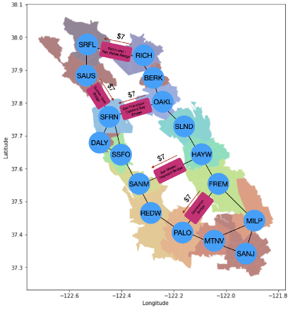
Figure 2: Bay Area transportation network with tolled bridge segments. Different colors on the map represent the boundaries of cities.

Demand estimate.

We categorize the driving population into three distinct segments based on their willingness-to-pay, namely low, middle, and high willingness-to-pay. The determination of the fraction of driving population in each of these categories relies on the Means of Transportation dataset from ACS. Specifically, we assign a traveler to the (a) low willingness-to-pay category if their annual individual income is less than $\$25,000$, to the (b) middle willingness-to-pay category if their annual individual income falls within the range of $\$25,000$ to $\$65,000$, and to the (c) high willingness-to-pay category if their annual individual income exceeds $\$65,000$.

Figure 3 provides a visual representation of the distribution of traveler demand to and from each node in the network, stratified by willingness-to-pay. It is essential to underscore that this demand specifically pertains to inter-node travel, with within-node demand excluded from the analysis. We describe the methodology employed for demand estimation in the next section. Moreover, we find that approximately 40% of travelers are high willingess-to-pay, and 30% of travelers are of middle and low willingness-to-pay, each.

In Figure 3(a) (resp. Figure 3(b)), we present the distribution of traveler demand based on their home (resp. work) location. Around $55\%$ of traffic emerges from relatively few nodes on the East Bay such as RICH, OAKL, SLND, HAYW, FREM, SANJ. Moreover, around $40\%$ of traffic has a work destination in one of the four nodes SFRN, PALO, MTNV, and OAKL. Notably, there exists substantial heterogeneity in both the home and work locations of different traveler types, as can be observed by comparing the distribution of demands in Figure 3 to the distribution of median income found in Figure 1(a). For instance, nodes such as RICH, HAYW, SLND, and DALY  are predominantly inhabited by a higher number of low willingness-to-pay  travelers, while nodes such as PALO, OAKL, SFRN, FREM, and SAUS  are predominantly inhabited by high willingness-to-pay travelers. It is interesting to note that on most of the nodes the demographics of incoming traffic predominantly comprise high willingness-to-pay travelers. Additionally, as can be seen in Figure 4, high-income travelers make up a large fraction demand that originates in the West Bay, as well as of the work location demand on both the East and West Bay.

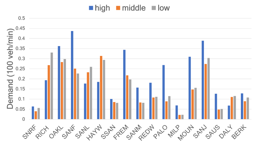
(a) Distribution of traveler types based on their origin (home) nodes.

(b) Distribution of traveler types based on their destination (work) nodes.

Figure 3: Distribution of origin and destination traveler demands.

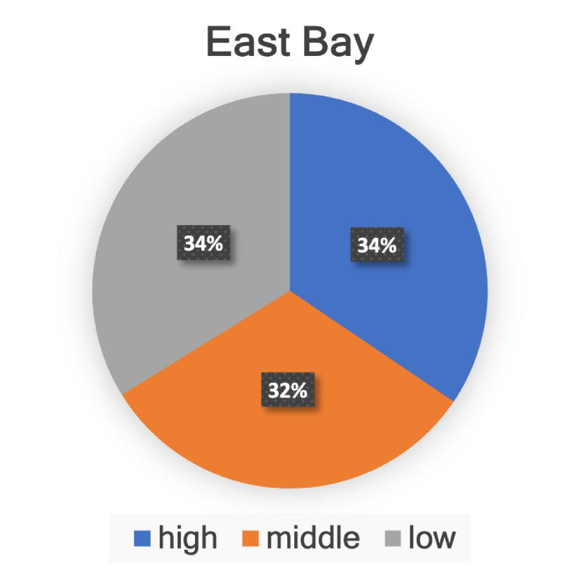
(a) Home Location

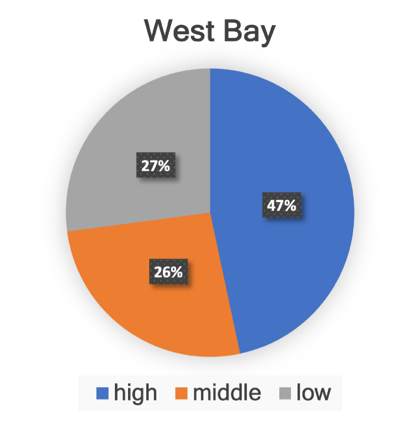
(b) Home Location

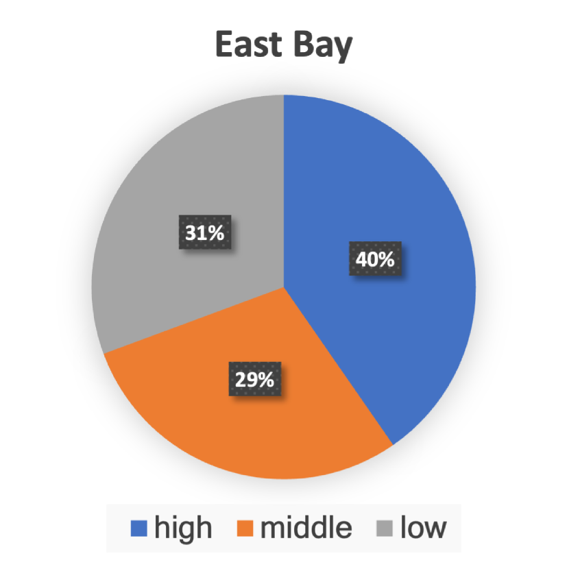
(c) Work Location

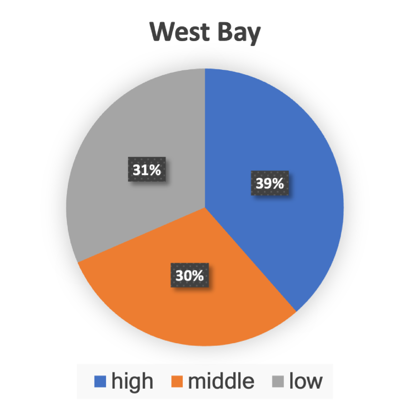
(d) Work Location

Figure 4: Distribution of demands across high, middle, and low income levels.

Next, we describe the approach used to compute the daily demand of different types of travelers traveling between different o-d pairs during January 2019-June 2019. There are three main steps to our approach: first, we obtain an estimate of the relative demand of travelers traveling between different zip-codes in the Bay Area by using the Safegraph dataset. Particularly, for every month, the Neighborhood Patterns data in the Safegraph dataset provides the average daily count of mobile devices that travel between different census block groups (CBGs) during the work day, which is then aggregated to obtain the relative demand of travelers traveling between different zip codes. After accounting for the sampling bias induced due to the randomly sampled population across the United States, we calibrate demands by using the ACS dataset which provides the income-stratified driving population in every zip code. Finally, to obtain an estimate of daily variability in demand we further augment the demand data with the PeMS dataset by adjusting for daily variation in the total flow on the network in every month. The details of demand estimation are included in Appendix C.

Calibrating the edge latency functions.

We calibrate the latency functions of each edge of the Bay Area freeway network shown in Figure 2. We adopt the Bureau of Public Roads (BPR) function proposed by the Federal Highway Administration (FHA) (Manual,, 1964) as follows:

$$\ell_{e}(w_{e})=a_{e}+b_{e}w_{e}^{4},\quad\forall\ e\in E,$$ (15)

where $a_{e}$ represents the free-flow travel time (i.e. latency with zero flow) of edge $e$ and $b_{e}$ is the slope of congestion.

We compute the average driving time of each edge during the morning rush hour (6am to 12pm) on each workday from January 1, 2019 to June 30, 2019 using the speed and distance data from the PeMS dataset. We denote the set of all days as $\mathcal{T}$, the average travel time and traffic flow of each edge $e\in E$ on day $t\in\mathcal{T}$ as $\hat{\ell}_{e}^{t}$ and $\hat{w}_{e}^{t}$, respectively. The details of computing $\left(\hat{\ell}_{e}^{t},\hat{w}_{e}^{t}\right)_{t\in\mathcal{T}}$ are provided in Appendix B. We estimate the free-flow travel time $a_{e}$ of each $e\in E$ using the average travel time of edge $e$ computed from the PeMS dataset at 3am, when the traffic flow is approaching zero. We denote the estimated value of $a_{e}$ as $\hat{a}_{e}$ for each $e\in E$. We next estimate the slope $b_{e}$ of each edge $e\in E$ using an ordinary least squares regression. In particular, the estimate $\hat{b}_{e}$ is solved as the minimizer of the following convex program:

$$\hat{b}_{e}=\underset{b_{e}\in\mathbb{R}}{\arg\min}\sum_{t\in\mathcal{T}}\|\hat{\ell}_{e}^{t}-\hat{a}_{e}-b_{e}\cdot(\hat{w}_{e}^{t})^{4}\|^{2},\quad\forall\ e\in E.$$

5.3 Estimating the willingness-to-pay parameters

We formulate the problem of estimating the willingness-to-pay parameters as an inverse optimization problem. Specifically, the optimal estimate of willingness-to-pay parameters corresponding to the three types of travelers, $\theta^{H*},\theta^{M*},\theta^{L*}$, are the ones that minimize the difference between the observed flows on each edge of the network and the corresponding equilibrium edge flows. That is,

$$\theta^{*}_{H},\theta^{*}_{M},\theta^{*}_{L} =\operatorname*{arg\,min}_{\begin{subarray}{c}\theta^{H},\theta^{M},\theta^{L}\end{subarray}}\quad\sum_{t\in\mathcal{T}}\sum_{e\in E}(\hat{w}_{e}^{t}-w_{e}(q^{t}))^{2}$$

s.t. $$q^{t}\in\underset{q\in\mathcal{Q}(D^{t})}{\arg\min}\ \Phi(q,p,\theta)\ \quad\forall t\in\mathcal{T},$$ (16a)

$$w_{e}(q^{t})$$ is given by (3), (16b)

$$\mathcal{Q}(D^{t})$$ is given by (1), (16c)

where $p$ is the toll price vector in 2019 (i.e. $\$7$ on each bridge, and $\$0$ for the remaining edges), $\hat{w}_{e}^{t}$ is the observed edge flow on each edge $e\in E$ and each day $t\in\mathcal{T}$ computed using the PeMS dataset, and $D^{t}$ is the estimated demand vector of each day $t$ computed using the ACS and Safegraph datasets.

Directly solving (16) is a challenging problem due to the non-linearity of the edge latency function and the potential function in (16a). We compute the estimates using grid search: we construct a grid of willingness to pay, where the granularity of each of $\theta^{H},\theta^{M},\theta^{L}$ is $\$5$ per hour. We also assume that the maximum value of willingness to pay is $\$100$ per hour and the minimum is $\$0$ per hour. Therefore, we define the set of all possible parameter values as $\Theta:=\{0,5,10,15,\dots,100\}^{3}$. For each $\theta=(\theta^{H},\theta^{M},\theta^{L})\in\Theta$, we compute the the equilibrium flow $q_{t}$ for every $t\in\mathcal{T}$ and compute the total squared error as in the objective function of (16). The optimal parameter $\theta^{\ast}$ is the one that minimizes the total squared error. We obtain:

$$\theta^{*}=(\theta^{L*},\theta^{M*},\theta^{H*})=(\$10/\text{hour},\ \$30/\text{hour},\ \$70/\text{hour}).$$ (17)

Our estimate $\theta^{*}$ is consistent with the observations reported in prior works, which show that the willingness-to-pay values typically lie between $60\%-100\%$ of the average hourly income of the population ((Palmquist et al.,, 2007; Athira et al.,, 2016; Meunier and Quinet,, 2015)).

Furthermore, as a robustness check, we plot the equilibrium edge flow $w_{e}(q^{t\ast})$ and observed edge flow $\hat{w}_{e}^{t}$ for every $e\in E,t\in\mathcal{T}$ in Figure 5. Each dot in this figure represents the flow on an edge $e\in E$ on a single day $t\in\mathcal{T}$. Overall, the dots are distributed along the diagonal of the plot indicating that the our computed equilibrium edge flow are relatively consistent with the observed edge flow subject to noise in time costs and demand fluctuations.

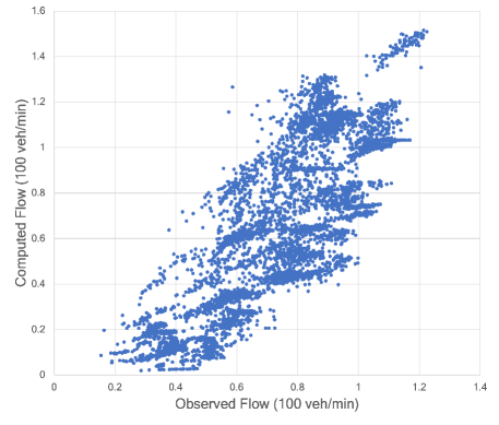
Figure 5: Comparison of observed flow and computed equilibrium edge flow.

6 Efficiency and equity analysis of congestion pricing schemes

Our goal in this section is three fold. First, we analyze the congestion levels induced at equilibrium due to current congestion pricing scheme, curr, and identify corridors in the Bay Area which are congested. Next, using the computational method introduced in Section 4 and the calibrated model of San Francisco Bay area freeway network in Section 5, we compute the toll values under the congestion pricing schemes hom, het, hom_sc, and het_sc. Finally, we compare different congestion pricing schemes in terms of efficiency and equity of travel cost, and also in terms of overall revenue generated at equilibrium.

6.1 Congestion under the current congestion pricing scheme (curr)

Here, we analyze the congestion levels induced at equilibrium under the current congestion pricing scheme, curr, which imposes a uniform toll of $7 on each of the five bridges in the Bay Area, namely on the Richmond-San Rafael Bridge (RICH-SRFL), San Francisco-Oakland Bay Bridge (OAKL-SFRN), Golden Gate Bridge (SAUS-SFRN), San Mateo-Hayward Bridge (HAYW-SANM), and Dumbarton Bridge (FREM-PALO).

Figure 6(a) depicts the difference between the equilibrium travel time given curr and the congestion minimizing travel time (normalized by free flow travel time on every edge). We observe that edges on the eastern corridor (connecting nodes RICH-BERK-OAKL-SLND-HAYW-FREM) are over-congested. Meanwhile, the edges on the western corridor (connecting nodes SRFL-SAUS-SFRN-DALY-SSFO-SANM-REDW) are relatively less congested. Furthermore, we observe that amongst all bridges the Bay Bridge (OAKL-SFRN) is also most congested, which is consistent with several prior studies (Nakamura and Kockelman,, 2002; Barnes et al.,, 2012; Gonzales and Christofa,, 2015). Additionally, Figure 6(b) presents the difference in the edge flows induced at equilibrium with that of socially optimal edge flows. We observe that in order to reduce the overall congestion we need to ensure that

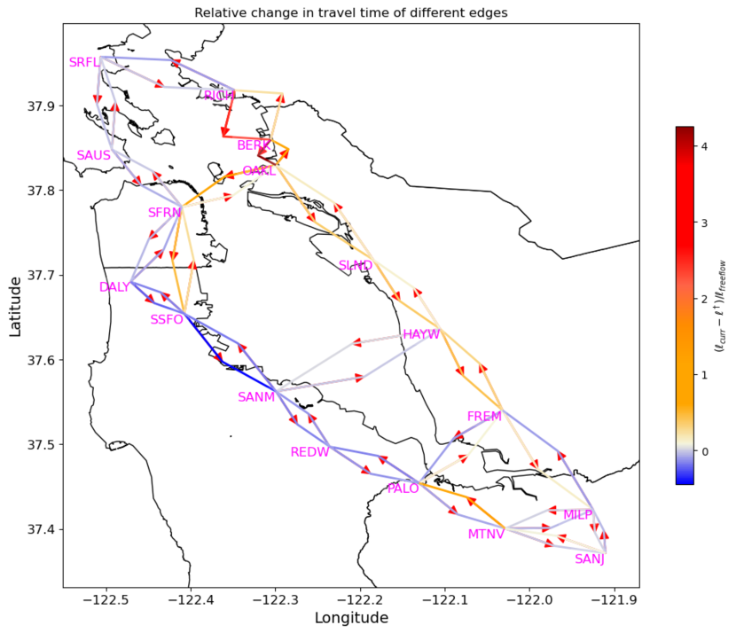
(a) Proportional travel time increase under curr (normalized by free flow travel time).

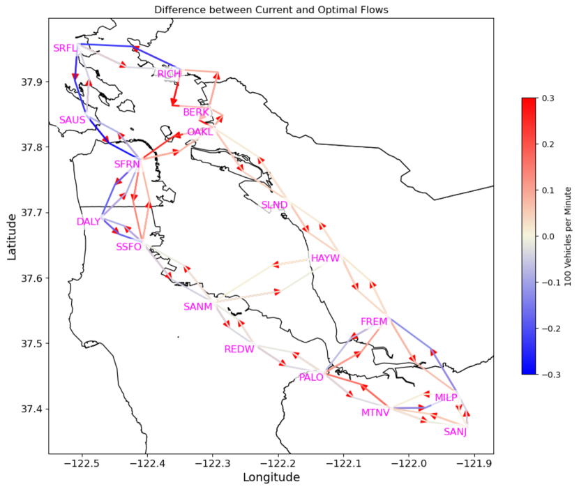
(b) Difference between equilibrium flow induced by curr and optimal flow.

Figure 6: Current congestion pricing scheme

1. the travelers using the edges in the corridor RICH-BERK-OAKL-SFRN (resp. SFRN-OAKL-BERK-RICH) are incentivized to use the edges in the corridor RICH-SRFL-SAUS-SFRN (resp. SFRN-SAUS-SRFL-RICH).

2. the travelers using the edges in the corridor SFRN-SSFO are incentivized to use the corridor SFRN-DALY-SSFO.

3. the travelers using the eastern corridor MILP-FREM-HAYW-SLND-OAKL are diverted to use the western corridor MTNV-PALO-REDW-SANM-SSFO by suitably incentivizing them to use the Dumbarton Bridge or the San Mateo-Hayward Bridge.

Furthermore, we note that the average travel cost (the sum of the travel time cost and the equivalent time cost of the monetary expense as in (4)) experienced by different types of travelers at equilibrium is unequal in curr. Specifically, low willingness-to-pay travelers bear the travel cost of approximately 91 minutes, while high and middle willingness-to-pay travelers face costs of 61 and 68 minutes, respectively. Moreover, as indicated in Table 2, this unequal distribution of travel time persists not only on average but also when examined across different threshold levels of travel cost.

Travel Cost	Low (% travelers)	Middle (% travelers)	High (% travelers)
more than 60 minutes	68	53	49
more than 90 minutes	50	34	27
more than 120 minutes	34	16	10
more than 150 minutes	18	2	1

Table 2: Fraction of low, middle and high willingness-to-pay travelers that incur total cost (in minutes) more than the threshold at equilibrium.

To summarize, we observe that the current congestion pricing scheme implemented the Bay area does not result in efficient allocation of traffic on the network. Additionally, it also leads to unequal distribution of travel cost across different types of travelers.

6.2 Toll values under different congestion pricing schemes

Here, using the calibrated model of the Bay area obtained in Section 5, we present the computed values of tolls on various edges of the Bay area network under different congestion pricing schemes (namely, hom, het, hom_sc, het_sc) obtained using the computational methodology presented in Section 4.

Figure 7(a) presents the toll values computed under hom by solving ($\mathcal{P}^{\ast}_{\textsf{hom}}$). Figures 7(b)-7(d) present the toll values for low, middle, and high willingness-to-pay travelers under het by solving ($\mathcal{P}^{\ast}_{\textsf{het}}$). Figure 7(e) presents the toll values computed under hom_sc by solving ($\mathcal{P}^{\ast}_{\textsf{hom\_sc}}$). Figure 7(f) further presents the toll values for low, middle, and high willingness-to-pay travelers under het_sc by solving ($\mathcal{P}^{\ast}_{\textsf{het\_sc}}$). To compute all of these toll values, we choose $\lambda=5$ in ($\mathcal{P}^{\ast}_{\textsf{hom}}$), ($\mathcal{P}^{\ast}_{\textsf{het}}$), ($\mathcal{P}^{\ast}_{\textsf{hom\_sc}}$), and ($\mathcal{P}^{\ast}_{\textsf{het\_sc}}$). This choice of parameter $\lambda$ ensures that the numerical value of the average welfare metric and the equity metric in these optimization problems are of the same order of magnitude.

Note that in hom and het, on all the bridges, tolls in the east-to-west direction are lower than tolls in the west-to-east direction. This is in contrast to curr, where the west-to-east direction is not tolled at all on any bridge and only the east-to-west direction is tolled at a flat rate of $\$7$ (refer Figure 2). Given that the western corridor is less congested than the eastern corridor in curr (refer Figure 6(a)), such tolling is useful to efficiently redistribute traffic in the network. Furthermore, note that in all of the congestion pricing schemes we compute, unlike curr, the Golden Gate Bridge (SAUS-SFRN) is not tolled at all. This choice ensures that more travelers in the eastern corridor, particularly in nodes such as RICHand BERK  are able to reach nodes in the west, particularly SFRN.

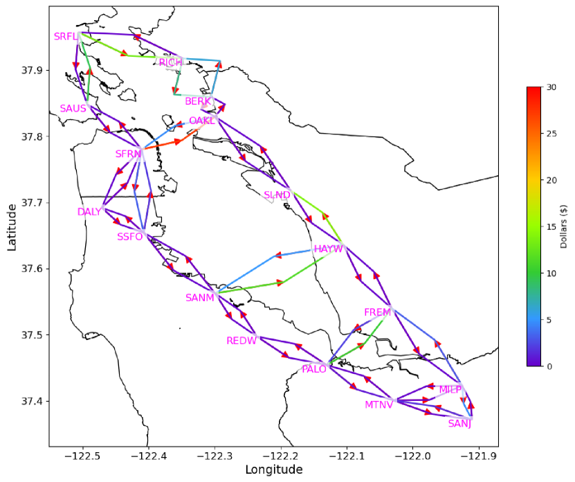
(a) Tolls under hom

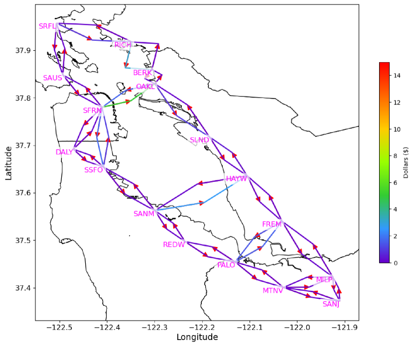
(b) Tolls under het for low type

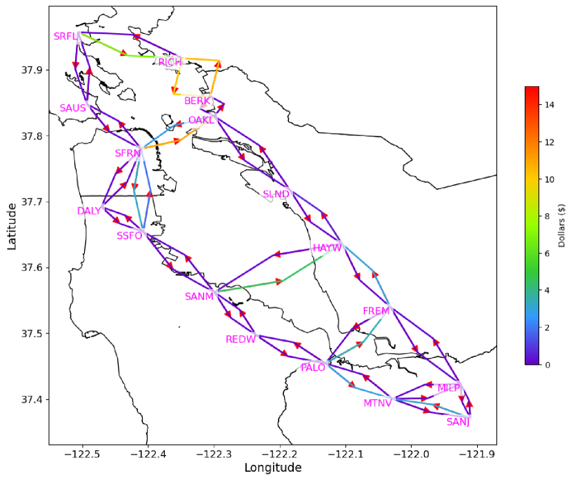
(c) Tolls under het for middle type

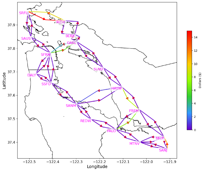
(d) Tolls under het for high type

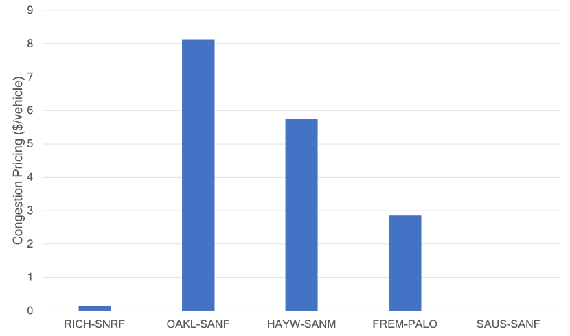
(e) Tolls under hom_sc 

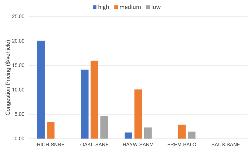
(f) Tolls under het_sc

Figure 7: Toll values under congestion pricing schemes hom, het, hom_sc, and het_sc.

6.3 Discussion on efficiency, equity and revenue generation

In this subsection, we compare the effectiveness of curr, hom, hom_sc, het and het_sc in terms of efficiency (the average travel time per traveler), equity (average total cost experienced by different types of travelers), and revenue generation (the total toll revenue generated by these schemes). Additionally, we also compare these pricing schemes with the scenario when no toll is implemented (denoted zero).

6.3.1 Efficiency Considerations.

Figure 8 represents the average travel time experienced by travelers under different congestion pricing schemes.

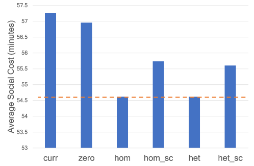
Figure 8: Comparison of average social cost per traveler for curr, zero, hom, hom_sc, het, and het_sc. Here, the orange dashed line represent congestion minimizing cost computed by solving (5).

As expected from Proposition 4.2, the congestion pricing schemes hom and het achieves the minimum congestion levels on the network. Additionally, we note that hom_sc and het_sc do not achieve the minimum congestion level due to the support constraints. Furthermore, it’s noteworthy that het_sc results in a slightly improved average travel time compared to hom_sc. This improvement can be attributed to the flexibility of heterogeneous pricing schemes, which allow for type-specific tolls.

From Figure 8, we observe that the price of anarchy – which is the ratio of the social cost of equilibrium congestion levels induced under no tolls with that of opt– is 1.04 for the Bay area transportation network. This is likely due to the high congestion level of the network during the morning rush hour. Indeed, theoretical studies (Colini-Baldeschi et al.,, 2020; Cominetti et al.,, 2021) have proved that the price of anarchy approaches to 1 as the total demand of travelers increases. Moreover, empirical studies (Youn et al.,, 2008; O’Hare et al.,, 2016) have also shown that the price of anarchy in the transportation networks of London, Boston and New York city are also close to 1.

We find that all congestion pricing schemes hom, hom_sc, het, het_sc outperform curr in terms of the average travel time. Surprisingly, it is also marginally outperformed by zero. A key reason is that curr imposes the same tolls on all of the bridges which does not result in effective re-distribution of traffic from eastern corridor to western corridor. While a reduced toll price or zero toll price may increase the total demand of travelers, but its impact is likely to be not significant due to (1) the high expense of car ownership and parking fee ((Depillis et al.,, 2023) estimates that US average annual car ownership cost is $12182 in 2023), and (2) the low coverage of public transportation in the Bay Area.

6.3.2 Equity considerations.

Figure 9 illustrates the average travel cost experienced by type of travelers under different pricing schemes. We observe that the difference of average cost across the three traveler types is lower in het, het_sc, hom_sc, and zero, in comparison to curr. Moreover, we observe that for all type of travelers, the average travel cost is lower in het, het_sc, hom_sc, and zero, in comparison to curr. Furthermore, we note that this observation not only holds in the averaged sense but also in a distributional sense as illustrated in Table 3, which presents the proportion of travelers of a particular type experiencing travel costs surpassing a predetermined threshold. We observe that, regardless of the value of threshold and the type of travelers, the proportion of travelers experiencing cost higher than a threshold is higher in curr in comparison to het, het_sc, hom_sc, and zero. This shows that all proposed alternative pricing schemes (except for hom) are more equitable than curr for every type of travelers. The pricing scheme hom results in higher travel cost because it charges higher tolls to travelers.

In homogeneous congestion pricing schemes, regardless of the threshold and the type of traveler, a higher percentage of travelers incur travel costs exceeding a set threshold compared to heterogeneous pricing. This is due to type-specific tolls in heterogeneous schemes resulting in lower tolls for travelers. Additionally, pricing schemes with support constraints reduce the percentage of travelers exceeding a threshold. While the differences are marginal between het and het_sc, such differences are more prominent between hom and hom_sc.

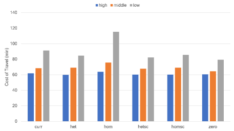
Figure 9: Average travel cost experienced by different types of travelers under different tolling schemes.

Travel Cost	curr	zero	het_sc	hom_sc	hom	het
more than 60 minutes	68%	60%	62%	63%	77%	67%
more than 90 minutes	50%	42%	44%	46%	60%	47%
more than 120 minutes	34%	26%	28%	29%	49%	29%
more than 150 minutes	18%	10%	11%	13%	35%	14%

(a) low willingness-to-pay travelers

Travel Cost	curr	zero	het_sc	hom_sc	hom	het
more than 60 minutes	53%	51%	54%	52%	61%	57%
more than 90 minutes	34%	31%	34%	32%	42%	34%
more than 120 minutes	16%	13%	11%	12%	20%	17%
more than 150 minutes	2%	1%	2%	2%	10%	4%

(b) middle willingness-to-pay travelers

Travel Cost	curr	zero	het_sc	hom_sc	hom	het
more than 60 minutes	49%	48%	47%	47%	51%	48%
more than 90 minutes	27%	26%	25%	25%	28%	25%
more than 120 minutes	10%	9%	9%	9%	12%	9%
more than 150 minutes	1%	0%	1%	0%	2%	1%

(c) high willingness-to-pay travelers

Table 3: Percentage of travelers with total cost (4) exceeding the threshold under each pricing scheme.

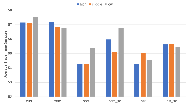
(a) Average travel time

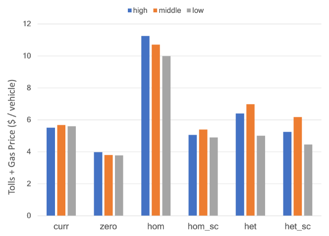
(b) Average monetary cost (tolls + gas price)

Figure 10: Average travel time and average monetary cost under curr, hom, het, hom_sc, het_scand zero.

Recall from (4) that the travel cost experienced by each traveler type includes the travel time cost and the equivalent time cost of monetary expenses (tolls and gas fee) assessed by the willingness-to-pay. Figure 10(a), which complements Figure 8, presents the average travel time under different congestion pricing scheme stratified by traveler types. Additionally, Figure 10(b) presents the average monetary cost (including both toll and gas prices) paid by each traveler type under different pricing schemes.

We observe that for every type of travelers, the travel time experienced under curr and zero is worse than any of the proposed pricing scheme. This arises from curr imposing uniform, non-zero tolls on all Bay Area bridges, a practice that overlooks the region’s geographic diversity in residential and workplace locations, as well as the significant socioeconomic disparities among its populations. By changing the pricing scheme to any one of the alternatives, we can reduce the average travel time of all three traveler types. Furthermore, we observe that for every type of travelers the average travel time experienced is higher in pricing schemes with support constraints than the ones without.

The average monetary cost of zero and hom_sc is lower than that of curr for every type of traveler. Moreover, het and het_sc results in higher monetary cost for high and medium types, and lower cost for the low type in comparison to curr. Additionally, it is evident that, for each traveler type, the average monetary cost experienced in hom is the highest compared to any other pricing scheme. This is attributed to hom imposing high tolls to ensure minimal congestion. However, the average monetary costs experienced in het are only slightly higher than those in other schemes, even though het minimizes congestion (refer Figure 8). This is due to type-specific toll prices in het which provides desired re-distribution of traffic with lower toll values.

6.3.3 Revenue considerations

Another important aspect of determining the congestion pricing scheme is the revenue it generates, which could be used for maintenance of existing transportation infrastructure, enhancing public transit options, amongst other things. Figure 11 presents a comparison of different congestion pricing scheme in terms of total revenue. As per the data released by Metropolitan Transportation Commission (MTC) a total toll revenue of $\$633,932,206$ was collected in the Bay Area during the year 2019-2020. Our calibrated model in curr predicts toll revenues on the same order of magnitude but slightly lower than MTC data. The mismatch between our prediction and MTC data is attributed to the fact that (i) our analysis only focuses on morning rush hour but MTC data also include tolls collected beyond morning rush hour as well, (ii) MTC data also includes tolls on HOV (High Occupancy Vehicle) lanes which are currently not added in our analysis, (iii) there is some additional demand incoming from other nearby cities not included in our analysis, and (iv) higher tolls are charged to multi-axle vehicles, with tolls charged as high as $\$36$ in 2019.

Notably, hom generates the highest revenue as it applies uniformly higher prices across all edges, irrespective of traveler types, with the goal of achieving a minimum congestion congestion level. Moreover, the revenue of the other three pricing schemes hom_sc, het and het_sc are comparable to that of curr with het being slightly higher and hom_sc and het_sc being slightly lower.

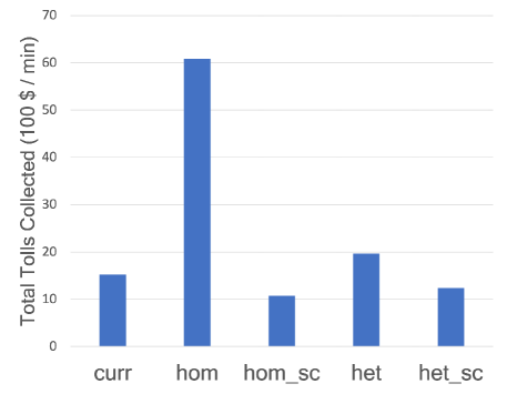
Figure 11: Comparison of total revenue collected for current,hom,hom-c,het,het-c.

7 Conclusion and discussion

We study the problem of designing congestion pricing schemes which not only minimize the overall congestion but also reduce the disparate impact of congestion pricing schemes on the basis of socioeconomic and geographic diversity of travelers. We present a multi-step linear programming based approach to design four kinds of congestion pricing schemes varying in terms of their implementation depending on whether (a) they can toll travelers on the basis of their willingness-to-pay, and (b) they can toll every edge of the network or only a subset of it. The evaluation and comparison of these congestion pricing schemes on the San Francisco Bay Area highway network reveal several significant insights. The proposed schemes outperform the currently implemented scheme in terms of overall congestion reduction and exhibit improvements in equity by providing better travel costs to each type of traveler. The analysis also highlights the revenue generation potential of different pricing schemes. Furthermore, heterogeneous pricing schemes can yield more equitable distribution of travel cost between different types of travelers, paving the way for future research to explore effective implementation strategies.

There are several interesting directions of future research. First, the implementation question inspires a study of the design of tax rebate programs that facilitate heterogeneous pricing schemes. Second, a more comprehensive empirical understanding of traffic patterns in the Bay Area can be done by incorporating travelers incoming from other cities in the Bay Area. Finally, it would be interesting to account for mode choice between driving and public transit, and more generally to account for elasticity of demand occurring from other choices such as remote work.

Appendix A Proofs for Section 4

Proof of Proposition 1.

• To establish this result, we first show that for any given set of tolls $p$, the optimization problem (6) is a convex optimization problem. Next, using KKT conditions for optimality we show that the optimal solution to (6) satisfy the requirements of Nash equilibrium posited in Definition 3.1.

  To show that the (6) is a convex optimization problem, we note that the constraint set is convex as it is a product simplex which is a convex set. Next, we show that the objective function is convex. Since the objective is differentiable, it is sufficient to show that

  $$\sum_{i\in I}\sum_{k\in K}\sum_{r\in R^{k}}\left(\frac{\partial\Phi(q,p)}{\partial q_{r}^{ik}}-\frac{\partial\Phi(\tilde{q},p)}{\partial q_{r}^{ik}}\right)\left(q_{r}^{ik}-\tilde{q}_{r}^{ik}\right)\geq 0\quad\forall\ q,\tilde{q}\in\mathcal{Q},q\neq\tilde{q}.$$ (18)

  To see this, we note that

  $$\frac{\partial\Phi(q,p)}{\partial q_{r}^{ik}} =\sum_{e\in E}\ell_{e}(w_{e}(q))\frac{\partial w_{e}(q)}{\partial q_{r}^{ik}}+\sum_{i\in I}\sum_{e\in E}\frac{(p_{e}^{i}+g_{e})}{\theta^{i}}\frac{\partial w_{e}^{i}(q)}{\partial q_{r}^{ik}}$$

  $$=\sum_{e\in E}\ell_{e}(w_{e}(q))\mathbbm{1}(e\in r)+\sum_{e\in E}\frac{(p_{e}^{i}+g_{e})}{\theta^{i}}\mathbbm{1}(e\in r)=c_{r}^{i}(q,p).$$

  Consequently, for any $q,\tilde{q}\in\mathcal{Q}$ such that $q\neq\tilde{q}$ it holds that

  $$\sum_{i\in I}\sum_{k\in K}\sum_{r\in R^{k}}\left(\frac{\partial\Phi(q,p)}{\partial q_{r}^{ik}}-\frac{\partial\Phi(\tilde{q},p)}{\partial q_{r}^{ik}}\right)\left(q_{r}^{ik}-\tilde{q}_{r}^{ik}\right)$$

  $$=\sum_{i\in I}\sum_{k\in K}\sum_{r\in R^{k}}\left(\sum_{e\in E}(\ell_{e}(w_{e}(q))-\ell_{e}(w_{e}(\tilde{q})))\mathbbm{1}(e\in r)\right)\left(q_{r}^{ik}-\tilde{q}_{r}^{ik}\right),$$

  $$=\sum_{e\in E}(\ell_{e}(w_{e}(q))-\ell_{e}(w_{e}(\tilde{q})))\sum_{i\in I}\sum_{k\in K}\sum_{r\in R^{k}}\mathbbm{1}(e\in r)\left(q_{r}^{ik}-\tilde{q}_{r}^{ik}\right),$$

  $$=\sum_{e\in E}(\ell_{e}(w_{e}(q))-\ell_{e}(w_{e}(\tilde{q})))\left(w_{e}(q)-w_{e}(\tilde{q})\right)\geq 0.$$

  where the last inequality follows because $\ell_{e}$ is strictly increasing function. Thus, we have established the (6) is convex optimization problem.

  Next, we analyze the KKT conditions associated with (6). Define the Lagrangian

  $$\mathcal{L}(q,\lambda,\mu;p)=\Phi(q,p)+\sum_{i\in I}\sum_{k\in K}\lambda^{ik}(D^{ik}-\sum_{r\in R^{k}}q_{r}^{ik})-\sum_{i\in I}\sum_{k\in K}\sum_{r\in R^{k}}\mu_{r}^{ik}q_{r}^{ik}.$$

  Since (6) is a convex optimization problem and the strong form of Slater’s conditions hold as the feasible set is a product-simplex, we obtain the following first-order necessary and sufficient condition of optimality:

  $$\frac{\partial\mathcal{L}(q^{\ast}(p),\lambda^{\ast},\mu^{\ast};p)}{\partial q_{r}^{ik}}=0\quad\forall\ i\in I,k\in K,r\in R^{k},$$ (C1)

  $$\sum_{r\in R^{k}}q_{r}^{*ik}(p)=D^{ik}\quad\forall\ i\in I,k\in K,$$ (C2)

  $$\mu_{r}^{*ik}q_{r}^{*ik}(p)=0\quad\forall\ i\in I,k\in K,r\in R^{k},$$ (C3)

  $$\mu_{r}^{*ik}\geq 0,q_{r}^{*ik}(p)\geq 0\quad\forall\ i\in I,k\in K,r\in R^{k}.$$ (C4)

  Note that (C1) can be equivalently written as

  $$0 =\frac{\partial\mathcal{L}(q^{\ast}(p),\lambda^{\ast},\mu^{\ast};p)}{\partial q_{r}^{ik}}=\frac{\partial\Phi(q^{\ast}(p),p)}{\partial q_{r}^{ik}}-\lambda^{ik}-\mu_{r}^{ik}=c_{r}^{i}(q^{\ast}(p),p)-\lambda^{ik}-\mu_{r}^{ik}$$

  Additionally, using (C4) we obtain that $c_{r}^{i}(q^{\ast}(p),p)\geq\lambda^{ik}$, for every $i\in I,k\in K,r\in R^{k}$. Furthermore, from (C3) we obtain that if for some $i\in I,k\in K,r\in R^{k}$, $q_{r}^{\ast ik}>0$ then $c_{r}^{i}(q^{\ast}(p),p)=\lambda^{ik}.$ This is precisely the conditions stated in Definition 3.1.

• Using the first-order necessary conditions for constrained optimality, we observe that,

  $$\sum_{i\in I}\sum_{k\in K}\sum_{r\in R^{k}}\frac{\partial S(q^{\dagger})}{\partial q_{r}^{ik}}\left(\tilde{q}_{r}^{ik}-q_{r}^{\dagger,ik}\right)\geq 0\quad\ \forall\ \tilde{q}\in\mathcal{Q}.$$ (19)

  Similarly, it holds that

  $$\sum_{i\in I}\sum_{k\in K}\sum_{r\in R^{k}}\frac{\partial S(\bar{q}^{\dagger})}{\partial q_{r}^{ik}}\left(\tilde{q}_{r}^{ik}-\bar{q}_{r}^{\dagger,ik}\right)\geq 0\quad\ \forall\ \tilde{q}\in\mathcal{Q}.$$ (20)

  Selecting $\tilde{q}=\bar{q}^{\dagger}$ in (19), and selecting $\tilde{q}=q^{\dagger}$ in (20) and substracting the resulting inequality we obtain

  $$\sum_{i\in I}\sum_{k\in K}\sum_{r\in R^{k}}\left(\frac{\partial S(q^{\dagger})}{\partial q_{r}^{ik}}-\frac{\partial S(\bar{q}^{\dagger})}{\partial q_{r}^{ik}}\right)\left({q}_{r}^{\dagger,ik}-\bar{q}_{r}^{\dagger,ik}\right)\leq 0.$$ (21)

  Suppose there exists $q^{\dagger},\bar{q}^{\dagger}\in Q^{\dagger}$ such that there exists $e\in E$ such that $w_{e}(q^{\dagger})\neq w_{e}(\bar{q}^{\dagger})$. Then we will show that (21) is violated.

  Note that for any $q\in\mathcal{Q}$,

  $$\frac{\partial S(q)}{\partial q_{r}^{ik}} =\sum_{e\in E}\frac{\partial w_{e}(q)}{\partial q_{r}^{ik}}\ell_{e}(w_{e}(q))+\sum_{e\in E}w_{e}(q)\nabla\ell_{e}(w_{e}(q))\frac{\partial w_{e}(q)}{\partial q_{r}^{ik}}$$

  $$=\sum_{e\in E}\mathbbm{1}(e\in r)\ell_{e}(w_{e}(q))+\sum_{e\in E}w_{e}(q)\nabla\ell_{e}(w_{e}(q))\mathbbm{1}(e\in r).$$

  Using this, we compute the left-hand side of (21),

  $$\sum_{i\in I}\sum_{k\in K}\sum_{r\in R^{k}}\left(\frac{\partial S(q^{\dagger})}{\partial q_{r}^{ik}}-\frac{\partial S(\bar{q}^{\dagger})}{\partial q_{r}^{ik}}\right)\left({q}_{r}^{\dagger,ik}-\bar{q}_{r}^{\dagger,ik}\right)$$

  $$= \sum_{i\in I}\sum_{k\in K}\sum_{r\in R^{k}}\sum_{e\in E}\mathbbm{1}(e\in r)(\ell_{e}(w_{e}(q^{\dagger}))-\ell_{e}(w_{e}(\bar{q}^{\dagger})))\left({q}_{r}^{\dagger,ik}-\bar{q}_{r}^{\dagger,ik}\right)$$

  $$\quad+\sum_{i\in I}\sum_{k\in K}\sum_{r\in R^{k}}\sum_{e\in E}(w_{e}(q^{\dagger})\nabla\ell_{e}(w_{e}(q^{\dagger}))-w_{e}(\bar{q}^{\dagger})\nabla\ell_{e}(w_{e}(\bar{q}^{\dagger})))\mathbbm{1}(e\in r)\left({q}_{r}^{\dagger,ik}-\bar{q}_{r}^{\dagger,ik}\right)$$

  $$= \sum_{e\in E}(\ell_{e}(w_{e}(q^{\dagger}))-\ell_{e}(w_{e}(\bar{q}^{\dagger})))\sum_{i\in I}\sum_{k\in K}\sum_{r\in R^{k}}\mathbbm{1}(e\in r)\left({q}_{r}^{\dagger,ik}-\bar{q}_{r}^{\dagger,ik}\right)$$

  $$\quad+\sum_{e\in E}(w_{e}(q^{\dagger})\nabla\ell_{e}(w_{e}(q^{\dagger}))-w_{e}(\bar{q}^{\dagger})\nabla\ell_{e}(w_{e}(\bar{q}^{\dagger})))\sum_{i\in I}\sum_{k\in K}\sum_{r\in R^{k}}\mathbbm{1}(e\in r)\left({q}_{r}^{\dagger,ik}-\bar{q}_{r}^{\dagger,ik}\right)$$

  $$= \sum_{e\in E}(\ell_{e}(w_{e}(q^{\dagger}))-\ell_{e}(w_{e}(\bar{q}^{\dagger})))\left(w_{e}(q^{\dagger})-w_{e}(\bar{q}^{\dagger})\right)$$

  $$\quad+\sum_{e\in E}(w_{e}(q^{\dagger})\nabla\ell_{e}(w_{e}(q^{\dagger}))-w_{e}(\bar{q}^{\dagger})\nabla\ell_{e}(w_{e}(\bar{q}^{\dagger})))\left(w_{e}(q^{\dagger})-w_{e}(\bar{q}^{\dagger})\right)$$

  Note that $\sum_{e\in E}(\ell_{e}(w_{e}(q^{\dagger}))-\ell_{e}(w_{e}(\bar{q}^{\dagger})))\left(w_{e}(q^{\dagger})-w_{e}(\bar{q}^{\dagger})\right)\geq 0,$ due to the monotonicity of latency function. Moreover, note that

  $$\sum_{e\in E}(w_{e}(q^{\dagger})\nabla\ell_{e}(w_{e}(q^{\dagger}))-w_{e}(\bar{q}^{\dagger})\nabla\ell_{e}(w_{e}(\bar{q}^{\dagger})))\left(w_{e}(q^{\dagger})-w_{e}(\bar{q}^{\dagger})\right)$$

  $$= \sum_{e\in E}(w_{e}(q^{\dagger})\nabla\ell_{e}(w_{e}(q^{\dagger}))-w_{e}(\bar{q}^{\dagger})\nabla\ell_{e}(w_{e}(q^{\dagger}))+w_{e}(\bar{q}^{\dagger})\nabla\ell_{e}(w_{e}(q^{\dagger}))-w_{e}(\bar{q}^{\dagger})\nabla\ell_{e}(w_{e}(\bar{q}^{\dagger})))\left(w_{e}(q^{\dagger})-w_{e}(\bar{q}^{\dagger})\right)$$

  $$= \sum_{e\in E}\nabla\ell_{e}(w_{e}(q^{\dagger}))(w_{e}(q^{\dagger})-w_{e}(\bar{q}^{\dagger}))^{2}+\sum_{e\in E}w_{e}(\bar{q}^{\dagger})(\nabla\ell_{e}(w_{e}(q^{\dagger}))-\nabla\ell_{e}(w_{e}(\bar{q}^{\dagger})))\left(w_{e}(q^{\dagger})-w_{e}(\bar{q}^{\dagger})\right).$$

  Note that $\sum_{e\in E}\nabla\ell_{e}(w_{e}(q^{\dagger}))(w_{e}(q^{\dagger})-w_{e}(\bar{q}^{\dagger}))^{2}>0$ due to the hypothesis that there exists at least one edge where $w_{e}(q^{\dagger})\neq w_{e}(\bar{q}^{\dagger})$ and the fact that the latency function is strictly increasing. Moreover $\sum_{e\in E}w_{e}(\bar{q}^{\dagger})(\nabla\ell_{e}(w_{e}(q^{\dagger}))-\nabla\ell_{e}(w_{e}(\bar{q}^{\dagger})))\left(w_{e}(q^{\dagger})-w_{e}(\bar{q}^{\dagger})\right)\geq 0$ as $\ell_{e}(\cdot)$ is assumed to be convex. Thus, we obtain

  $$\sum_{i\in I}\sum_{k\in K}\sum_{r\in R^{k}}\left(\frac{\partial S(q^{\dagger})}{\partial q_{r}^{ik}}-\frac{\partial S(\bar{q}^{\dagger})}{\partial q_{r}^{ik}}\right)\left({q}_{r}^{\dagger,ik}-\bar{q}_{r}^{\dagger,ik}\right)>0,$$

  which contradicts (21).

$\square$

Proof of Proposition 4.2.

(1) First, we prove that given any optimal solution $(p^{\dagger},z^{\dagger})$ of ($\mathcal{P}_{\textsf{hom}}$), $p^{\dagger}$ induces the socially optimal edge flow vector $w^{\dagger}$. Consider any optimal solution of ($\mathcal{D}_{\textsf{hom}}$), denoted as $q^{\dagger}$. From strong duality theory, we know that $(p^{\dagger},z^{\dagger},q^{\dagger})$ must satisfy complementary slackness conditions associated with the constraints in ($\mathcal{P}_{\textsf{hom}}$) and ($\mathcal{D}_{\textsf{hom}}$). In particular, the complementary slackness condition for ($\mathcal{P}_{\textsf{hom}}$)-($\mathcal{D}_{\textsf{hom}}$) indicates that for any $i\in I$, $k\in K$, and $r\in R^{k}$,

$$q^{\dagger ik}_{r}>0,\quad\Rightarrow\quad z^{\dagger ik}=\theta^{i}\ell_{r}(w^{\dagger})+\sum_{e\in r}(p_{e}^{\dagger}+g_{e})=\theta^{i}c_{r}^{i}(q^{\dagger},p^{\dagger}).$$

Additionally, from ($\mathcal{P}_{\textsf{hom}}$), we have for all $i\in I,k\in K,r^{\prime}\in R^{k}$,

$$z^{\dagger ik}\leq\theta^{i}\ell_{r^{\prime}}(w^{\dagger})+\sum_{e\in r^{\prime}}(p_{e}^{\dagger}+g_{e})=\theta^{i}c_{r^{\prime}}^{i}(q^{\dagger},p^{\dagger}).$$

Consequently,

$$\forall i\in I,k\in K,r\in R^{k},\quad q^{\dagger ik}_{r}>0,\quad\Rightarrow\quad c_{r}^{i}(q^{\dagger},p^{\dagger})\leq c_{r^{\prime}}^{i}(q^{\dagger},p^{\dagger}),\quad\forall r^{\prime}\in R_{k}.$$ (22)

That is, the flow vector $q^{\dagger}$ only takes routes with the minimum cost given the socially optimal edge flow vector $w^{\dagger}$. We next prove that $w^{\dagger}$ is indeed induced by $q^{\dagger}$, i.e. constraint ($\mathcal{D}_{\textsf{hom}.a}$) is tight with the optimal solution.

For notational brevity, we denote $\hat{w}_{e}=\sum_{i\in I}\sum_{k\in K}\sum_{r\in\{R^{k}|r\ni e\}}q_{r}^{\dagger ik}$ as the edge flow induced by $q^{\dagger}$. Suppose for the sake of contradiction that for some non-empty subset of edges $E^{\dagger}\subseteq E$,

$$\forall\ e\in E^{\dagger},\quad\hat{w}_{e}=\sum_{i\in I}\sum_{k\in K}\sum_{r\in\{R^{k}|r\ni e\}}q_{r}^{\dagger ik}<w_{e}^{\dagger},$$

$$\forall\ e\in E\backslash E^{\dagger},\quad\hat{w}_{e}=\sum_{i\in I}\sum_{k\in K}\sum_{r\in\{R^{k}|r\ni e\}}q_{r}^{\dagger ik}=w_{e}^{\dagger}.$$

Then,

$$\sum_{e\in E}\hat{w}_{e}\ell_{e}(\hat{w}_{e})=\sum_{e\in E^{\dagger}}\hat{w}_{e}\ell_{e}(\hat{w}_{e})+\sum_{e\in E\backslash E^{\dagger}}\hat{w}_{e}\ell_{e}(\hat{w}_{e})<\sum_{e\in E^{\dagger}}w_{e}^{\dagger}\ell_{e}(w_{e}^{\dagger})+\sum_{e\in E\backslash E^{\dagger}}w_{e}^{\dagger}\ell_{e}(w_{e}^{\dagger})=\sum_{e\in E}w_{e}^{\dagger}\ell_{e}(w_{e}^{\dagger}),$$

where the inequality is due the the fact that $\ell_{e}$ is a strictly increasing function. This contradicts with the fact that $w^{\dagger}$ minimizes the social cost function. Therefore, we must have $\hat{w}_{e}=\sum_{i\in I}\sum_{k\in K}\sum_{r\in\{R^{k}|r\ni e\}}f_{r}^{\dagger ik}=w_{e}^{\dagger}$, for every $e\in E$.

Following from the fact that $q^{\dagger}$ satisfies (22) and induces the socially optimal edge flow vector $w^{\dagger}$, we can conclude that $w^{\dagger}$ is an equilibrium edge flow vector induced by the flow vector $q^{\dagger}$ associated under the toll price $p^{\dagger}$. Hence, the optimal solution $p^{\dagger}$ of ($\mathcal{P}_{\textsf{hom}}$) indeed implements the socially optimal edge flow.

We now prove the other direction. Suppose that there exists a $\hom$ toll vector $\tilde{p}$ that induces the socially optimal edge flow $w^{\dagger}$ in equilibrium, then there exists $\tilde{z}$ such that $(\tilde{z},\tilde{p})$ is an optimal solution to ($\mathcal{P}_{\textsf{hom}}$). We denote $\tilde{q}$ as a Nash equilibrium strategy distribution given toll $\tilde{p}$. Then, such $\tilde{q}$ is a feasible solution of ($\mathcal{D}_{\textsf{hom}}$), and ($\mathcal{D}_{\textsf{hom}.a}$) holds with equality.

Next, we define $\tilde{z}^{ik}=\min_{r\in R^{k}}\theta^{i}\tilde{\ell}_{r}(w^{\dagger})+\sum_{e\in r}(\tilde{p}_{e}+g_{e})$. This ensures that

$$\tilde{z}^{ik}\leq\theta^{i}\tilde{\ell}_{r}(w^{\dagger})+\sum_{e\in r}(\tilde{p}_{e}+g_{e}),\quad\forall k\in K,r\in R^{k},i\in I.$$

Therefore, $(\tilde{p},\tilde{z})$ is a feasible solution of the primal problem ($\mathcal{P}_{\textsf{hom}}$). Moreover, we note that $(\tilde{p},\tilde{z},\tilde{q})$ satisfies the complementary slackness condition associated with ($\mathcal{P}_{\textsf{hom}}$) and ($\mathcal{D}_{\textsf{hom}}$). Thus, $(\tilde{p},\tilde{z})$ is an optimal solution to ($\mathcal{P}_{\textsf{hom}}$) and $\tilde{q}$ is an optimal solution to ($\mathcal{D}_{\textsf{hom}}$).

(2) The proof of this part follows an analogous procedure as that in part (1). We denote an optimal solution of ($\mathcal{P}_{\textsf{het}}$) as $(p^{\dagger},z^{\dagger})$, and an optimal solution of ($\mathcal{D}_{\textsf{het}}$) as $q^{\dagger}$. From the complementary slackness condition associated with ($\mathcal{P}_{\textsf{het}}$)-($\mathcal{D}_{\textsf{het}}$), we know that if $q^{\dagger ik}_{r}>0$ for some $i\in I,k\in K,r\in R^{k}$, then $z^{\dagger ik}=\theta^{i}\tilde{\ell}_{r}(w^{\dagger})+\sum_{e\in r}(p_{e}^{\dagger i}+g_{e})=\theta^{i}c_{r}^{i}(q^{\dagger},p^{\dagger})$. Moreover, we know that for every $i\in I,k\in K,r^{\prime}\in R^{k}$,

$$z^{\dagger ik}\leq\theta^{i}\tilde{\ell}_{r^{\prime}}(w^{\dagger})+\sum_{e\in r^{\prime}}(p_{e}^{\dagger i}+g_{e})=\theta^{i}c_{r^{\prime}}^{i}(q,p^{\dagger}),$$

which implies that $c_{r}^{i}(q^{\dagger},p^{\dagger})\leq c_{r^{\prime}}^{i}(q^{\dagger},p^{\dagger})$, i.e. $q^{\dagger}$ sends flow on routes with the minimum cost associated with the heterogeneous toll $p^{\dagger}$ and the socially optimal edge flow $w^{\dagger}$. Moreover, following the same procedure as that in the $\hom$ case, we can argue that $q^{\dagger}$ induces the socially optimal edge flow $f^{\dagger}$ (i.e. ($\mathcal{D}_{\textsf{het}.a}$) is tight), otherwise we arrive at a contradiction that $f^{\dagger}$ is not socially optimal. Therefore, we can conclude that $q^{\dagger}$ is an equilibrium strategy distribution that induces the socially optimal (type-specific) edge flow $f^{\dagger}$ given the het toll vector $p^{\dagger}$.

On the other hand, suppose that there exists a het toll vector $\tilde{p}$ that induces the socially optimal edge flow $w^{\dagger}$in equilibrium, then we define $\tilde{z}^{ik}=\min_{r\in R^{k}}\theta^{i}\ell_{r}(w^{\dagger})+\sum_{e\in r}(\tilde{p}^{i}_{e}+g_{e})$ for all $k\in K$, $r\in R^{k}$, and $i\in I$. Analogous to the case with $\hom$ toll, we can argue that $(\tilde{p},\tilde{z})$ (resp. $\tilde{q}$ ) is a feasible solution of ($\mathcal{P}_{\textsf{het}}$) (resp. ($\mathcal{D}_{\textsf{het}}$)), and satisfies complementary slackness conditions. Consequently, we know that $(\tilde{p},\tilde{z})$ (resp. $\tilde{q}$ ) is an optimal solution of ($\mathcal{P}_{\textsf{het}}$) (resp. ($\mathcal{D}_{\textsf{het}}$)). $\square$

Appendix B Latency function calibration

Here, we present the methodology used to compute the latency function of all freeways in Figure 2. Recall from Section 5, we need to compute the average travel time and average flow on every edge for every day. To achieve this goal, we utilize morning rush hour data from the PeMS dataset, spanning from January 2019 to June 2019. Let’s denote the set of all weekdays in this time-frame by $\mathcal{T}$. For every edge $e\in E$ and day $t\in\mathcal{T}$, let’s denote the average travel time by $\hat{\ell}_{e}^{t}$ and the average edge flow by $\hat{w}_{e}^{t}$. In order to estimate these quantities, we use PeMS data during the morning rush hours $\mathcal{H}=[6\text{am}-7\text{am},7\text{am}-8\text{am},8\text{am}-9\text{am},9\text{am}-10\text{am},10\text{am}-11\text{am},11\text{am}-12\text{noon}]$. Let $S_{e}$ be the number of sensors fitted on edge $e\in E$ which provide average hourly flow and average speed information.

First, we demonstrate how to use the raw data from sensors to compute the average travel time on every edge. We compute an estimate of the time required to travel the edge $e$ at hour $h$ by accumulating the average time required to travel between sensors on that link as follows:

$$\hat{\ell}_{e}^{ht}=\sum_{s=1}^{S_{e}-1}\frac{L_{e}^{s}}{v_{e}^{sht}},\quad\forall\ e\in E,h\in\mathcal{H},t\in\mathcal{T},$$ (23)

where $L_{e}^{s}$ is the distance between sensor $s$ and $s+1$ on edge $e\in E$ and $v_{e}^{sht}$ is the average speed of traffic passing over the sensor $s$ on edge $e$ during hour $h$ on day $t$. Next, we compute the average hourly flow on an edge as follows:

$$\hat{w}_{e}^{ht}=\frac{\sum_{s=1}^{S_{e}-1}L_{e}^{s}\tilde{w}_{e}^{sht}}{\sum_{s=1}^{S_{e}-1}L_{e}^{s}},\quad\forall\ e\in E,h\in\mathcal{H},t\in\mathcal{T},$$

where $\tilde{w}_{e}^{sht}$ is the hourly average flow of traffic passing over sensor $s$ on edge $e$ during hour $h$ on day $t$. We use the hourly average edge flows $\hat{w}_{e}^{ht}$ and the hourly average travel times $\hat{\ell}_{e}^{ht}$ to compute the average travel time on any edge $e\in E$ as follows:

$$\hat{\ell}_{e}^{t}=\frac{\sum_{h\in\mathcal{H}}\hat{w}_{e}^{ht}\hat{\ell}_{e}^{ht}}{\sum_{h\in\mathcal{H}}\hat{w}_{e}^{ht}},\quad e\in E,t\in\mathcal{T}.$$

Similarly, we compute the average of the hourly flows as follows:

$$\hat{w}_{e}^{t}=\frac{1}{|\mathcal{H}|}\sum_{h\in\mathcal{H}}\hat{w}_{e}^{ht},\quad t\in\mathcal{T},e\in E.$$

Appendix C Demand computation

We outline our method for calculating the daily demand of travelers moving between various origin-destination pairs from January 2019 to June 2019. Our approach involves three main steps:

Step 1: Estimating relative demand between nodes using the Safegraph dataset:

We leverage the Safegraph dataset to obtain the relative demand of travelers traveling between different nodes in the Bay Area. Specifically, the Neighborhood Patterns dataset from Safegraph provides the average daily count of mobile devices moving between different census block groups (CBGs) on workdays for each month. This is then aggregated over the set of nodes after adjusting for sampling bias.

More formally, let’s denote the set of CBGs in the Bay Area by $\mathcal{C}$. The SafeGraph dataset provides the average daily count of travelers $N^{cc^{\prime}}$ traveling from CBG $c$ to $c^{\prime}$. However, the SafeGraph dataset exhibits sampling bias because different CBGs are sampled at different rates. We correct for sampling bias in this data by modifying the counts $N^{cc^{\prime}}$ using the population data provided by the ACS. That is, we compute the corrected count of travelers traveling from CBG $c$ to $c^{\prime}$ as follows

$$\tilde{N}^{cc^{\prime}}=N^{cc^{\prime}}\frac{R^{c}}{\sum_{c\in\mathcal{C}}R^{c}}\cdot\frac{\sum_{c\in\mathcal{C}}\sum_{c^{\prime}\in\mathcal{C}}N^{cc^{\prime}}}{\sum_{c^{\prime}\in\mathcal{C}}N^{cc^{\prime}}},$$

where $R^{c}$ is the number of residents in CBG $c$ as reported by the ACS dataset.

Step 2: Calibrating type-specific demands with ACS dataset.

Given the the adjusted count of travelers we compute the demand of travelers from o-d pair $k\in K$ by aggregating the demand over set of nodes as follows

$$\tilde{D}^{k}=\sum_{c\in k_{o}}\sum_{c^{\prime}\in k_{d}}\tilde{N}_{\mathcal{C}}^{cc^{\prime}},$$

where $k_{o},k_{d}\in N$ are the origin and destination nodes of the o-d pair $k\in K$. To obtain the demand in terms of units of flow we compute

$$D^{ik}=\frac{\tilde{D}^{k}}{\sum_{k^{\prime}\in K}\tilde{D}^{k^{\prime}}\mathbbm{1}(k^{\prime}_{o}=k_{o})}\frac{A^{ik_{o}}}{|\mathcal{H}|},$$

where $A^{ik_{o}}$ is the total driving population of type $i$ at node $k_{o}$ as given by the ACS dataset and $|\mathcal{H}|$ is the number of hours in morning rush hours (6 am to 12 noon).

Step 3: Incorporating daily variability with the PeMS dataset.

We convert the monthly demand estimates obtained in Step 2 into daily demand data by scaling it proportional to the total daily flow from PeMS dataset. More formally, we compute the average total edge load over all workdays from January 2019 to June 2019 as follows

$$\overline{w}=\frac{1}{|\mathcal{T}|}\sum_{t\in\mathcal{T}}\sum_{e\in E}\hat{w}_{e}^{t},$$ (24)

where $\hat{w}_{e}^{t}$ is the average edge load on day $t$ on edge $e$, which is obtained in Appendix B using PeMS data. Next, to obtain the daily demand, we scale the monthly demand obtain in Step 2 as follows:

$$D^{ik}_{t}=\frac{\sum_{e\in E}\hat{w}_{e}^{t}}{\overline{w}}\cdot D^{ik},\quad\forall\ t\in\mathcal{T},i\in I,k\in K.$$ (25)

References

- Adler and Cetin, (2001) Adler, J. L. and Cetin, M. (2001). A direct redistribution model of congestion pricing. Transportation research part B: methodological, 35(5):447–460.
- Angelelli et al., (2016) Angelelli, E., Arsik, I., Morandi, V., Savelsbergh, M., and Speranza, M. G. (2016). Proactive route guidance to avoid congestion. Transportation Research Part B: Methodological, 94:1–21.
- Angelelli et al., (2021) Angelelli, E., Morandi, V., Savelsbergh, M., and Speranza, M. G. (2021). System optimal routing of traffic flows with user constraints using linear programming. European journal of operational research, 293(3):863–879.
- Arnott and Small, (1994) Arnott, R. and Small, K. (1994). The economics of traffic congestion. American scientist, 82(5):446–455.
- Athira et al., (2016) Athira, I., Muneera, C., Krishnamurthy, K., and Anjaneyulu, M. (2016). Estimation of value of travel time for work trips. Transportation Research Procedia, 17:116–123. International Conference on Transportation Planning and Implementation Methodologies for Developing Countries (12th TPMDC) Selected Proceedings, IIT Bombay, Mumbai, India, 10-12 December 2014.
- Bai et al., (2004) Bai, L., Hearn, D. W., and Lawphongpanich, S. (2004). Decomposition techniques for the minimum toll revenue problem. Networks: An International Journal, 44(2):142–150.
- Bai et al., (2010) Bai, L., Hearn, D. W., and Lawphongpanich, S. (2010). A heuristic method for the minimum toll booth problem. Journal of Global Optimization, 48(4):533–548.
- Bai and Rubin, (2009) Bai, L. and Rubin, P. A. (2009). Combinatorial benders cuts for the minimum tollbooth problem. Operations research, 57(6):1510–1522.
- Barnes et al., (2012) Barnes, I. C., Frick, K. T., Deakin, E., and Skabardonis, A. (2012). Impact of peak and off-peak tolls on traffic in san francisco–oakland bay bridge corridor in california. Transportation research record, 2297(1):73–79.
- Beckmann et al., (1956) Beckmann, M., McGuire, C. B., and Winsten, C. B. (1956). Studies in the economics of transportation. Technical report.
- Bergendorff et al., (1997) Bergendorff, P., Hearn, D. W., and Ramana, M. V. (1997). Congestion toll pricing of traffic networks. Springer.
- Bernstein, (1993) Bernstein, D. (1993). Congestion pricing with tolls and subsidies. In Pacific Rim TransTech Conference—Volume II: International Ties, Management Systems, Propulsion Technology, Strategic Highway Research Program, pages 145–151. ASCE.
- Bonifaci et al., (2011) Bonifaci, V., Salek, M., and Schäfer, G. (2011). Efficiency of restricted tolls in non-atomic network routing games. In Algorithmic Game Theory: 4th International Symposium, SAGT 2011, Amalfi, Italy, October 17-19, 2011. Proceedings 4, pages 302–313. Springer.
- Brotcorne et al., (2001) Brotcorne, L., Labbé, M., Marcotte, P., and Savard, G. (2001). A bilevel model for toll optimization on a multicommodity transportation network. Transportation science, 35(4):345–358.
- Brown and Marden, (2016) Brown, P. N. and Marden, J. R. (2016). A study on price-discrimination for robust social coordination. In 2016 American Control Conference (ACC), pages 1699–1704. IEEE.
- Cole et al., (2003) Cole, R., Dodis, Y., and Roughgarden, T. (2003). Pricing network edges for heterogeneous selfish users. In Proceedings of the thirty-fifth annual ACM symposium on Theory of computing, pages 521–530.
- Colini-Baldeschi et al., (2020) Colini-Baldeschi, R., Cominetti, R., Mertikopoulos, P., and Scarsini, M. (2020). When is selfish routing bad? the price of anarchy in light and heavy traffic. Operations Research, 68(2):411–434.
- Cominetti et al., (2021) Cominetti, R., Dose, V., and Scarsini, M. (2021). The price of anarchy in routing games as a function of the demand. Mathematical Programming, pages 1–28.
- Craik and Balakrishnan, (2023) Craik, L. and Balakrishnan, H. (2023). Equity impacts of the london congestion charging scheme: an empirical evaluation using synthetic control methods. Transportation research record, 2677(5):1017–1029.
- Depillis et al., (2023) Depillis, L., Lieberman, R., and Chapman, C. (2023). How the costs of car ownership add up.
- Dial, (2000) Dial, R. B. (2000). Minimal-revenue congestion pricing part ii: An efficient algorithm for the general case. Transportation Research Part B: Methodological, 34(8):645–665.
- DOT, (2008) DOT, U. (2008). Income-Based Equity Impacts of Congestion Pricing.
- Ekström et al., (2009) Ekström, J., Engelson, L., and Rydergren, C. (2009). Heuristic algorithms for a second-best congestion pricing problem. NETNOMICS: Economic Research and Electronic Networking, 10:85–102.
- Eliasson, (2001) Eliasson, J. (2001). Road pricing with limited information and heterogeneous users: A successful case. The annals of regional science, 35:595–604.
- Eliasson and Mattsson, (2006) Eliasson, J. and Mattsson, L.-G. (2006). Equity effects of congestion pricing: quantitative methodology and a case study for stockholm. Transportation Research Part A: Policy and Practice, 40(7):602–620.
- Feng et al., (2023) Feng, R., Zhang, H., Shi, B., Zhong, Q., and Yao, B. (2023). Collaborative road pricing strategy for heterogeneous vehicles considering emission constraints. Journal of Cleaner Production, 429:139561.
- Ferrari, (2002) Ferrari, P. (2002). Road network toll pricing and social welfare. Transportation Research Part B: Methodological, 36(5):471–483.
- Fleischer et al., (2004) Fleischer, L., Jain, K., and Mahdian, M. (2004). Tolls for heterogeneous selfish users in multicommodity networks and generalized congestion games. In 45th Annual IEEE Symposium on Foundations of Computer Science, pages 277–285. IEEE.
- Frick et al., (1996) Frick, K. T., Heminger, S., and Dittmar, H. (1996). Bay bridge congestion-pricing project: Lessons learned to date. Transportation Research Record, 1558(1):29–38.
- Gonzales and Christofa, (2015) Gonzales, E. J. and Christofa, E. (2015). Empirical assessment of bottleneck congestion with a constant and peak toll: San francisco–oakland bay bridge. EURO Journal on Transportation and Logistics, 3(3):267–288.
- Goodwin, (1990) Goodwin, P. (1990). How to make road pricing popular. Economic Affairs, 10(5):6–7.
- Gunn, (2001) Gunn, H. (2001). Spatial and temporal transferability of relationships between travel demand, trip cost and travel time. Transportation Research Part E: Logistics and Transportation Review, 37(2-3):163–189.
- Guo and Yang, (2010) Guo, X. and Yang, H. (2010). Pareto-improving congestion pricing and revenue refunding with multiple user classes. Transportation Research Part B: Methodological, 44(8-9):972–982.
- Han et al., (2022) Han, L., Peng, C., and Xu, Z. (2022). The effect of commuting time on quality of life: evidence from china. International journal of environmental research and public health, 20(1):573.
- Harks et al., (2015) Harks, T., Kleinert, I., Klimm, M., and Möhring, R. H. (2015). Computing network tolls with support constraints. Networks, 65(3):262–285.
- Hearn and Ramana, (1998) Hearn, D. W. and Ramana, M. V. (1998). Solving congestion toll pricing models. Springer.
- Hoefer et al., (2008) Hoefer, M., Olbrich, L., and Skopalik, A. (2008). Taxing subnetworks. In International workshop on internet and network economics, pages 286–294. Springer.
- Jahn et al., (2005) Jahn, O., Möhring, R. H., Schulz, A. S., and Stier-Moses, N. E. (2005). System-optimal routing of traffic flows with user constraints in networks with congestion. Operations research, 53(4):600–616.
- Jalota et al., (2021) Jalota, D., Solovey, K., Gopalakrishnan, K., Zoepf, S., Balakrishnan, H., and Pavone, M. (2021). When efficiency meets equity in congestion pricing and revenue refunding schemes. In Equity and Access in Algorithms, Mechanisms, and Optimization, pages 1–11.
- Jalota et al., (2023) Jalota, D., Solovey, K., Tsao, M., Zoepf, S., and Pavone, M. (2023). Balancing fairness and efficiency in traffic routing via interpolated traffic assignment. Autonomous Agents and Multi-Agent Systems, 37(2):32.
- Kalashnikov et al., (2016) Kalashnikov, V. V., Herrera Maldonado, R. C., Camacho-Vallejo, J.-F., and Kalashnykova, N. I. (2016). A heuristic algorithm solving bilevel toll optimization problems. The International Journal of Logistics Management, 27(1):31–51.
- Karakostas and Kolliopoulos, (2004) Karakostas, G. and Kolliopoulos, S. G. (2004). Edge pricing of multicommodity networks for heterogeneous selfish users. In FOCS, volume 4, pages 268–276.
- Labbé et al., (1998) Labbé, M., Marcotte, P., and Savard, G. (1998). A bilevel model of taxation and its application to optimal highway pricing. Management science, 44(12-part-1):1608–1622.
- Larsson and Patriksson, (1998) Larsson, T. and Patriksson, M. (1998). Side constrained traffic equilibrium models—traffic management through link tolls. In Equilibrium and advanced transportation modelling, pages 125–151. Springer.
- Lawphongpanich and Hearn, (2004) Lawphongpanich, S. and Hearn, D. W. (2004). An mpec approach to second-best toll pricing. Mathematical programming, 101(1):33–55.
- Lawphongpanich and Yin, (2007) Lawphongpanich, S. and Yin, Y. (2007). Pareto-improving congestion pricing for general road networks. Technique Report. Gainesville, FL: Department of industrial and System Engineering, University of Florida.
- Lawphongpanich and Yin, (2010) Lawphongpanich, S. and Yin, Y. (2010). Solving the pareto-improving toll problem via manifold suboptimization. Transportation Research Part C: Emerging Technologies, 18(2):234–246.
- Lazar and Pedarsani, (2020) Lazar, D. A. and Pedarsani, R. (2020). Optimal tolling for multitype mixed autonomous traffic networks. IEEE Control Systems Letters, 5(5):1849–1854.
- Lazar and Pedarsani, (2021) Lazar, D. A. and Pedarsani, R. (2021). The role of differentiation in tolling of traffic networks with mixed autonomy. arXiv preprint arXiv:2103.13553.
- LeBeau, (2019) LeBeau, P. (2019). Traffic jams cost us $87 billion in lost productivity in 2018, and boston and dc have the nation’s worst.
- Lim, (2002) Lim, A. C. (2002). Transportation network design problems: An MPEC approach. The Johns Hopkins University.
- Liu, (2020) Liu, J. (2020). Commuters in this city spend 119 hours a year stuck in traffic.
- Manual, (1964) Manual, T. A. (1964). For application with a large, high speed computer.
- Mehr and Horowitz, (2019) Mehr, N. and Horowitz, R. (2019). Pricing traffic networks with mixed vehicle autonomy. In 2019 American Control Conference (ACC), pages 2676–2682. IEEE.
- Meunier and Quinet, (2015) Meunier, D. and Quinet, E. (2015). Value of time estimations in cost benefit analysis: the french experience. Transportation Research Procedia, 8:62–71.
- Nakamura and Kockelman, (2002) Nakamura, K. and Kockelman, K. M. (2002). Congestion pricing and roadspace rationing: an application to the san francisco bay bridge corridor. Transportation Research Part A: Policy and Practice, 36(5):403–417.
- O’Hare et al., (2016) O’Hare, S. J., Connors, R. D., and Watling, D. P. (2016). Mechanisms that govern how the price of anarchy varies with travel demand. Transportation Research Part B: Methodological, 84:55–80.
- Palmquist et al., (2007) Palmquist, R., Phaneuf, D., and Smith, V. K. (2007). Measuring the values for time.
- Patriksson and Rockafellar, (2002) Patriksson, M. and Rockafellar, R. T. (2002). A mathematical model and descent algorithm for bilevel traffic management. Transportation Science, 36(3):271–291.
- Percoco, (2015) Percoco, M. (2015). Heterogeneity in the reaction of traffic flows to road pricing: a synthetic control approach applied to milan. Transportation, 42:1063–1079.
- Phang and Toh, (2004) Phang, S.-Y. and Toh, R. S. (2004). Road congestion pricing in singapore: 1975 to 2003. Transportation Journal, pages 16–25.
- Pigou, (1912) Pigou, A. C. (1912). Wealth and welfare. Macmillan and Company, limited.
- Roughgarden, (2010) Roughgarden, T. (2010). Algorithmic game theory. Communications of the ACM, 53(7):78–86.
- Sheffi, (1984) Sheffi, Y. (1984). Urban Transportation Networks: Equilibrium Analysis With Mathematical Programming Methods.
- Small, (1992) Small, K. A. (1992). Using the revenues from congestion pricing. Transportation, 19:359–381.
- Smith, (1979) Smith, M. (1979). The marginal cost taxation of a transportation network. Transportation Research Part B: Methodological, 13(3):237–242.
- Song et al., (2009) Song, Z., Yin, Y., and Lawphongpanich, S. (2009). Nonnegative pareto-improving tolls with multiclass network equilibria. Transportation Research Record, 2091(1):70–78.
- Thomas and Thompson, (1970) Thomas, T. C. and Thompson, G. I. (1970). The value of time for commuting motorists as a function of their income level and amount of time saved. Highway Research Record, (314).
- Verhoef, (2002) Verhoef, E. T. (2002). Second-best congestion pricing in general networks. heuristic algorithms for finding second-best optimal toll levels and toll points. Transportation Research Part B: Methodological, 36(8):707–729.
- Waters, (1994) Waters, W. G. (1994). The value of travel time savings and the link with income: implications for public project evaluation. International Journal of Transport Economics/Rivista internazionale di economia dei trasporti, pages 243–253.
- Yang and Huang, (2004) Yang, H. and Huang, H.-J. (2004). The multi-class, multi-criteria traffic network equilibrium and systems optimum problem. Transportation Research Part B: Methodological, 38(1):1–15.
- Yang and Lam, (1996) Yang, H. and Lam, W. H. (1996). Optimal road tolls under conditions of queueing and congestion. Transportation Research Part A: Policy and Practice, 30(5):319–332.
- Yildirim and Hearn, (2005) Yildirim, M. B. and Hearn, D. W. (2005). A first best toll pricing framework for variable demand traffic assignment problems. Transportation Research Part B: Methodological, 39(8):659–678.
- Youn et al., (2008) Youn, H., Gastner, M. T., and Jeong, H. (2008). Price of anarchy in transportation networks: efficiency and optimality control. Physical review letters, 101(12):128701.
- Zhang and Batterman, (2013) Zhang, K. and Batterman, S. (2013). Air pollution and health risks due to vehicle traffic. Science of the total Environment, 450:307–316.
- Zhang et al., (2011) Zhang, L., Du, H., and Lee, L. (2011). Congestion pricing study of san francisco–oakland bay bridge in california. Transportation research record, 2221(1):83–95.