Coseparable Nonnegative Tensor Factorization with T-CUR Decomposition

Abstract

Nonnegative Matrix Factorization (NMF) is an important unsupervised learning method to extract meaningful features from data. To address the NMF problem within a polynomial time framework, researchers have introduced a separability assumption, which has recently evolved into the concept of coseparability. This advancement offers a more efficient core representation for the original data. However, in the real world, the data is more natural to be represented as a multi-dimensional array, such as images or videos. The NMF’s application to high-dimensional data involves vectorization, which risks losing essential multi-dimensional correlations. To retain these inherent correlations in the data, we turn to tensors (multidimensional arrays) and leverage the tensor t-product. This approach extends the coseparable NMF to the tensor setting, creating what we term coseparable Nonnegative Tensor Factorization (NTF). In this work, we provide an alternating index selection method to select the coseparable core. Furthermore, we validate the t-CUR sampling theory and integrate it with the tensor Discrete Empirical Interpolation Method (t-DEIM) to introduce an alternative, randomized index selection process. These methods have been tested on both synthetic and facial analysis datasets. The results demonstrate the efficiency of coseparable NTF when compared to coseparable NMF.

1 Introduction

In data science, unsupervised learning plays an important role in dealing with unlabeled data, which can find the unseen patterns, features, and structures of the data. Nonnegative Matrix Factorization (NMF) is a significant unsupervised learning method to extract meaningful features from data [4]. Given a nonnegative matrix $A\in\mathbb{R}_{\geq 0}^{m\times n}$ and a target rank $r<\min\{m,n\}$, NMF approximates $A$ by the product of two non-negative low-rank matrices: the dictionary matrix $W\in\mathbb{R}_{+}^{m\times r}$ and the coding matrix $H\in\mathbb{R}_{+}^{r\times n}$ i.e., $A\approx WH$. An important application of NMF is topic modeling, which can extract and classify topics from the given word-document data [25, 24, 34]. It can be used for tasks like text mining, sentiment analysis, and news clustering. To solve the NMF problem in polynomial time, a separability assumption is proposed in [10], i.e., $W$ is composed of some columns of $A$. Then some researchers proposed many algorithms to solve the separable NMF problem [2, 15, 12]. Recently, Pan and Ng generalized the separability assumption into the coseparability in [29], which assumes that $W$ is composed of some rows and columns of $A$. In other words, $W$ is a submatrix of $A$. It provides a more compact core matrix to represent the original data matrix $A$.

For high-dimensional data like images or videos, employing Non-negative Matrix Factorization (NMF) for clustering or feature extraction necessitates vectorization. However, this vectorization process can potentially disrupt inherent correlations in higher dimensions. For instance, converting an image into a vector might result in the loss of relational context between adjacent pixels. So we aim to find a similar method that can process them while preserving their high-dimensional structure. In recent years, tensors have been widely studied as a structure for high-dimensional data and different techniques have been studied. The CANDECOMP/PARAFAC (CP) and Tucker decompositions [23, 20, 33] can be considered to be higher-order generalizations of the matrix singular value decomposition (SVD). Oseledets developed tensor train decomposition [28] and Zhao et al. introduced tensor ring decomposition [36]. Another type of tensor factorization which is useful in applications called tensor t-product is founded by Kilmer and Martin in [22]. Based on the t-product, the matrix factorizations can be extended to tensors, such as t-SVD [22], t-QR/t-LU decomposition[37], and t-Schur decomposition [27, 7]. Han et. al. recently proposed an adaptive data augmentation framework based on the t-product in [18]. The matrix CUR decomposition, as it can utilize the self-expression to reduce the size of the initial matrix, is widely investigated in [26, 5, 32], and it was extended as t-CUR decompositions in [8].

In the tensor t-product framework, NMF has also been extended to a high-dimensional setting called nonnegative tensor factorization (NTF) [19]. Further studies in NTF can be found in [31]. In this paper, we want to extend the coseparability into higher dimensional cases, so we also use the t-product to establish the coseparable NTF theory.

The contribution of this paper can be summarized as follows.

1. We extend the coseparable NMF to tensors and propose coseparable NTF. Some of its properties have also been proven, including its relationship with t-CUR decomposition. To solve the coseparable NTF problem, An alternating index selection algorithm is proposed to choose the coseparable core.

2. Inspired by matrix CUR sampling theory, we present the t-CUR sampling theory, which is randomly sampling indices according to different probability distributions can achieve the t-CUR decomposition with high probability. Then, combining it with the tensor Discrete Empirical Interpolation Method (t-DEIM) [1], an alternative TCUR-DEIM method is proposed to select coseparable cores.

3. We test two methods on synthetic coseparable tensor data sets. We also test them on several real facial data sets and compare them with some matrix index selection methods.

The structure of this paper is as follows: Section 2 introduces the concept of tensor t-product. Our theoretical contributions regarding Coseparable Non-negative Tensor Factorization (CoS-NTF) are detailed in Section 3. Additionally, Section 4 presents the index selection algorithm for identifying the subtensor of the original tensor. Numerical validations of our theoretical results are provided in Section 5. The paper concludes with Section 6.

2 Preliminaries

2.1 Notations

In this paper, we adopt the following notation for clarity and consistency. Matrices are denoted by uppercase italic letters (e.g., $A$), while third-order tensors are represented by uppercase cursive italics (e.g., $\mathcal{A}$). The space of nonnegative matrices and third-order tensors is symbolized as $\mathbb{R}^{m\times n\times p}_{+}$ (with $\mathbb{R}^{m\times n}_{+}=\mathbb{R}^{m\times n\times 1}_{+}$ for matrices). We use $\{a:a+n\}$ to represent the integer set $\{a,a+1,\cdots,a+n\}$. $\mathcal{A}_{ijk}$ denotes the $(i,j,k)$-th entry of tensor $\mathcal{A}$ and $\mathcal{A}_{\mathbf{IJK}}$ denotes the subtensor of $\mathcal{A}$ whose entries $\mathcal{A}_{ijk}$ satisfy $i\in\mathbf{I}$, $j\in\mathbf{J}$, $k\in\mathbf{K}$ for sets $\mathbf{I,J,K}$. Specifically, $\mathcal{A}_{:jk}$ refers to $\mathcal{A}_{1:m,j,k}$. The cardinality of a set $\mathbf{s}$ is expressed as $|\mathbf{s}|$.

For matrix operations, $A^{\top}$ and $A^{\ast}$ denote the transpose and conjugate transpose of $A$, respectively. The inverse and Moore-Penrose pseudoinverse of $A$ are represented by $A^{-1}$ and $A^{{\dagger}}$. The Kronecker product of matrices $A$ and $B$ is indicated as $A\otimes B$. Norms are specified as $\|\cdot\|_{2}$ for the matrix spectral norm and $\|\cdot\|_{\mathrm{F}}$ for the Frobenius norm. $I_{n}$ denotes the $n\times n$ identity matrix, while $F_{n}$ signifies the $n\times n$ discrete Fourier transform (DFT) matrix, defined as:

$$F_{n}=\frac{1}{\sqrt{n}}\left(f_{jk}\right),\;f_{jk}=\omega_{n}^{jk},\;\omega_{n}=\mathrm{e}^{-\frac{2\pi\iota}{n}},\;\iota=\sqrt{-1}.$$

We also use functions in MATLAB to denote some operations: $\widehat{\mathcal{A}}:=\mathsf{fft}(\mathcal{A},[],3)$ and $\mathcal{A}:=\mathsf{ifft}(\widehat{\mathcal{A}},[],3)$ for the Fast Fourier Transform (FFT) and the inverse FFT along the third dimension of tensors $\mathcal{A}$ and $\widehat{\mathcal{A}}$, respectively. $\mathsf{diag}(\mathbf{v})$ denotes the diagonal matrix formed by array $\mathbf{v}=(v_{1},v_{2},\cdots,v_{n})$.

If $\mathsf{rank}\left(A\right)=r$, then the Singular Value Decomposition (SVD) of $A\in\mathbb{R}^{m\times n}$ can be represented as

$$A=W\Sigma V^{\top},$$

where $\Sigma=\mathsf{diag}\left(\sigma_{1}\left(A\right),\sigma_{2}\left(A\right),\cdots,\sigma_{r}\left(A\right),0,\cdots,0\right)$, $\sigma_{1}\left(A\right)\geqslant\sigma_{2}\left(A\right)\geqslant\ldots\geqslant\sigma_{r}\left(A\right)>0$, with $\sigma_{i}\left(A\right)$ being the $i$-th singular value, $W$ and $V$ are the left and right singular vector matrices of $A$. We denote $\sigma_{\min}\left(A\right)$ as the smallest nonzero singular value for convenience.

In the context of this paper, which extends the concept of coseparable NMF to tensors, we define coseparable NMF for reference as follows.

Definition 2.1.

A matrix ${A}\in\mathbb{R}^{m\times n}_{+}$ is co-$(r_{1},r_{2})$ separable if there exists index sets $\mathbf{I}$, $\mathbf{J}$ and matrices ${P}_{1}\in\mathbb{R}^{m\times r_{1}}_{+}$, ${P}_{2}\in\mathbb{R}^{r_{2}\times n}_{+}$ such that ${A}={P}_{1}{A}_{\mathbf{I}\mathbf{J}}{P}_{2}$, where $|\mathbf{I}|=r_{1}$, $|\mathbf{J}|=r_{2}$, $\left({P}_{1}\right)_{\mathbf{I}:}={I}_{r_{1}}$ and $\left({P}_{2}\right)_{:\mathbf{J}}={I}_{r_{2}}$. ${A}_{\mathbf{I}\mathbf{J}}$ is referred to as the core of matrix ${A}$.

2.2 Tensor t-product

A tensor can be regarded as a high-dimensional array. As shown in Figure 1, the left-hand side is an $m\times n\times p$ third-order tensor. Figure 1 (a), (b), and (c) are called row, column, and tube fibers respectively; (d), (e), and (f) are called horizontal, lateral, and frontal slices respectively.

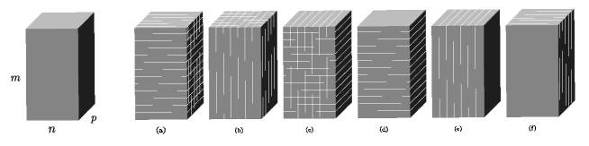
Figure 1: Illustration of a third-order tensor

The addition and subtraction of two $m\times n\times p$ tensors $\mathcal{A}$ and $\mathcal{B}$ is defined as

(1) $$\left(\mathcal{A}\pm\mathcal{B}\right)_{ijk}:=\mathcal{A}_{ijk}\pm\mathcal{B}_{ijk},\quad i\in\{1:m\},\ j\in\{1:n\},\ k\in\{1:p\}.$$

In preparation for defining the tensor t-product, we need operations $\mathsf{bcirc}$, $\mathsf{unfold}$ and $\mathsf{fold}$.

Definition 2.2.

([22]) Let $\mathcal{A}\in\mathbb{R}^{m\times n\times p}$. Then

(2) $${\mathsf{bcirc}}(\mathcal{A}):=\left[\begin{matrix}\mathcal{A}_{::1}&\mathcal{A}_{::p}&\cdots&\mathcal{A}_{::2}\\ \mathcal{A}_{::2}&\mathcal{A}_{::1}&\cdots&\mathcal{A}_{::3}\\ \vdots&\vdots&\ddots&\vdots\\ \mathcal{A}_{::p}&\mathcal{A}_{::,p-1}&\cdots&\mathcal{A}_{::1}\\ \end{matrix}\right],\quad{\mathsf{unfold}}(\mathcal{A}):=\left[\begin{array}[]{c}\mathcal{A}_{::1}\\ \mathcal{A}_{::2}\\ \vdots\\ \mathcal{A}_{::p}\\ \end{array}\right],\quad{\mathsf{fold}(\mathsf{unfold}}(\mathcal{A})):=\mathcal{A},$$

where ${\mathsf{bcirc}}(\mathcal{A})$ is called the block circulant matrix generated by $\mathcal{A}$.

Definition 2.3.

([22], T-product) The t-product of $\mathcal{A}\in\mathbb{R}^{m\times n\times p}$ and $\mathcal{B}\in\mathbb{R}^{n\times q\times p}$ is denoted as $\mathcal{A}\ast\mathcal{B}\in\mathbb{R}^{m\times q\times p}$ and

(3) $$\mathcal{A}\ast\mathcal{B}:=\mathsf{fold}\left(\mathsf{bcirc}\left(\mathcal{A}\right)\mathsf{unfold}\left(\mathcal{B}\right)\right).$$

The $\mathsf{bcirc}\left(\mathcal{A}\right)$ can be transformed into the Fourier domain as a block diagonal matrix [22]

(4) $$\left(F_{p}\otimes I_{m}\right)\mathsf{bcirc}\left(\mathcal{A}\right)\left(F_{p}^{\ast}\otimes I_{n}\right):=\widehat{A}=\left[\begin{matrix}\widehat{A}_{1}&&&\\ &\widehat{A}_{2}&&\\ &&\ddots&\\ &&&\widehat{A}_{p}\\ \end{matrix}\right].$$

Note that (3) is equivalent to $\mathsf{bcirc}\left(\mathcal{A}\ast\mathcal{B}\right)=\mathsf{bcirc}\left(\mathcal{A}\right)\mathsf{bcirc}\left(\mathcal{B}\right)$, then

(5) $$\left(F_{p}\otimes I_{m}\right)\mathsf{bcirc}\left(\mathcal{A}\ast\mathcal{B}\right)\left(F_{p}^{\ast}\otimes I_{q}\right)=\left(F_{p}\otimes I_{m}\right)\mathsf{bcirc}\left(\mathcal{A}\right)\mathsf{bcirc}\left(\mathcal{B}\right)\left(F_{p}^{\ast}\otimes I_{q}\right)=\widehat{A}\widehat{B},$$

which means the t-product can be computed in the Fourier domain. We have summarized the details of tensor t-product in Algorithm 1.

More precisely, we can fold the diagonal blocks $\widehat{A}_{k}$ in (4) into a tensor $\widehat{\mathcal{A}}$ such that $\widehat{\mathcal{A}}_{::k}=\widehat{A}_{k}$, which is equivalent to applying the FFT along the third dimension of $\mathcal{A}$, i.e., $\widehat{\mathcal{A}}=\mathsf{fft}(\mathcal{A},[],3)$. The same procedure is applied to $\mathcal{B}$, then we can perform matrix multiplication for their corresponding frontal slices in the complex domain. Consequently, the t-product can be efficiently computed using the FFT, as shown in Algorithm 1.

Algorithm 1 Tensor t-product

  $\mathbf{input}\ \mathcal{A}\in\mathbb{R}^{m\times n\times p}$ and $\mathcal{B}\in\mathbb{R}^{n\times q\times p}$

  $\widehat{\mathcal{A}}=\mathsf{fft}\left(\mathcal{A},\left[\right],3\right)$

  $\widehat{\mathcal{B}}=\mathsf{fft}\left(\mathcal{B},\left[\right],3\right)$

  for $k=1:p$ do

     $\widehat{\mathcal{C}}\left(:,:,k\right)=\widehat{\mathcal{A}}\left(:,:,k\right)\widehat{\mathcal{B}}\left(:,:,k\right)$

  end for

  ${\mathcal{C}}=\mathsf{ifft}\left(\widehat{\mathcal{C}},\left[\right],3\right)$

  return  $\mathcal{C}=\mathcal{A}\ast\mathcal{B}$

Now we review some definitions and technical results in the tensor t-product framework that will be used in the following sections.

Definition 2.4.

([22], Identity tensor) A tensor $\mathcal{I}\in\mathbb{R}^{n\times n\times p}$ is the identity tensor, if $\mathcal{I}_{::1}=I_{n}$ and $\mathcal{I}_{::k}=0\in\mathbb{R}^{n\times n}$, the zero matrix for $k\in\{2:p\}$.

Definition 2.5.

([22], Transpose and orthogonal tensor)
$\mathrm{(a)}$ The transpose of $\mathcal{A}\in\mathbb{R}^{m\times n\times p}$ is $\mathcal{A}^{\top}\in\mathbb{R}^{n\times m\times p}$, where $\left(\mathcal{A}^{\top}\right)_{::1}=\left(\mathcal{A}_{::1}\right)^{\top}$, $\left(\mathcal{A}^{\top}\right)_{::k}=\left(\mathcal{A}_{::,p-k+2}\right)^{\top}$, $k\in\{2:p\}$.
$\mathrm{(b)}$ A tensor $\mathcal{A}\in\mathbb{R}^{m\times n\times p}$ is orthogonal, if $\mathcal{A}^{\top}\ast\mathcal{A}=\mathcal{A}\ast\mathcal{A}^{\top}=\mathcal{I}$, where $\mathcal{I}$ is the identity tensor, see Definition 2.4.

Definition 2.6.

([22, 3], Inverse and Moore-Penrose inverse)
$\mathrm{(a)}$ A tensor $\mathcal{A}^{-1}\in\mathbb{R}^{n\times n\times p}$ is the inverse of $\mathcal{A}\in\mathbb{R}^{n\times n\times p}$, if $\mathcal{A}\ast\mathcal{A}^{-1}=\mathcal{A}^{-1}\ast\mathcal{A}=\mathcal{I}$, the identity tensor.
$\mathrm{(b)}$ A tensor $\mathcal{A}^{{\dagger}}\in\mathbb{R}^{n\times m\times p}$ is the Moore-Penrose inverse of $\mathcal{A}\in\mathbb{R}^{m\times n\times p}$, if $\mathcal{A}^{{\dagger}}$ satisfies the following equations,

$$\mathcal{A}\ast\mathcal{A}^{{\dagger}}\ast\mathcal{A}=\mathcal{A},\quad\mathcal{A}^{{\dagger}}\ast\mathcal{A}\ast\mathcal{A}^{{\dagger}}=\mathcal{A}^{{\dagger}},\quad\left(\mathcal{A}\ast\mathcal{A}^{{\dagger}}\right)^{\top}=\mathcal{A}\ast\mathcal{A}^{{\dagger}},\quad\left(\mathcal{A}^{{\dagger}}\ast\mathcal{A}\right)^{\top}=\mathcal{A}^{{\dagger}}\ast\mathcal{A}.$$

Definition 2.7.

([22, 32], Tensor norm) The Frobenius norm and the spectral norm of tensor $\mathcal{A}\in\mathbb{R}^{m\times n\times p}$ are defined as

(6) $$\lVert\mathcal{A}\rVert_{\mathrm{F}}:=\sqrt{\sum_{k}{\lVert\mathcal{A}_{::k}\rVert^{2}_{\mathrm{F}}}}=\sqrt{\sum_{i,j,k}{\left|\mathcal{A}_{ijk}\right|^{2}}},\quad\lVert\mathcal{A}\rVert_{2}:=\lVert\widehat{A}\rVert_{2}.$$

Remark 2.8.

Definition 2.3 indicates that $\left\|\mathsf{bcirc}\left(\mathcal{A}\right)\right\|_{\mathrm{F}}^{2}=p\left\|\mathcal{A}\right\|_{\mathrm{F}}^{2}$. Since the Frobenius norm is unitarily invariant, we can use (4) to derive

(7) $$p\left\|\mathcal{A}\right\|_{\mathrm{F}}^{2}=\left\|\left(F_{p}\otimes I_{m}\right)\mathsf{bcirc}\left(\mathcal{A}\right)\left(F_{p}^{\ast}\otimes I_{n}\right)\right\|_{\mathrm{F}}^{2}=\left\|\widehat{A}\right\|_{\mathrm{F}}^{2}=\sum_{k=1}^{p}{\left\|\widehat{A}_{k}\right\|_{\mathrm{F}}^{2}}=\sum_{k=1}^{p}{\left\|\widehat{\mathcal{A}}_{::k}\right\|_{\mathrm{F}}^{2}}=\left\|\widehat{\mathcal{A}}\right\|_{\mathrm{F}}^{2}.$$

We call a tensor f-diagonal if each of its frontal slices is a diagonal matrix [22]. In the t-product framework, the tensor still has its SVD, called t-SVD, which can factorize a tensor into two orthogonal tensors and an f-diagonal tensor.

Theorem 2.9.

([22], T-SVD) A tensor $\mathcal{A}\in\mathbb{R}^{m\times n\times p}$ can be decomposed by

(8) $$\mathcal{A}=\mathcal{W}\ast\varSigma\ast\mathcal{V}^{\top},$$

where $\mathcal{W}\in\mathbb{R}^{m\times m\times p}$ and $\mathcal{V}\in\mathbb{R}^{n\times n\times p}$ are orthogonal and $\varSigma$ is f-diagonal.

Now we will introduce the tensor multirank and the tensor tubalrank, where the multirank guarantees the t-CUR decomposition, and the tubalrank is useful in the t-CUR sampling theory in the following sections.

Definition 2.10.

([35], Multirank and tubalrank)
$\mathrm{(a)}$ Let the tensor $\mathcal{A}\in\mathbb{R}^{m\times n\times p}$ satisfy $\mathsf{rank}\left(\widehat{A}_{k}\right)=r_{k}$, $k\in\{1:p\}$, then the multirank of $\mathcal{A}$, denoted as $\mathsf{rank}_{m}\left(\mathcal{A}\right)$, is defined as the vector $\mathbf{r}=\left(r_{1},r_{2},\cdots,r_{p}\right)$.
$\mathrm{(b)}$ Let $\mathcal{A}=\mathcal{W}\ast\varSigma\ast\mathcal{V}^{\top}$ be the t-SVD of $\mathcal{A}\in\mathbb{R}^{m\times n\times p}$, then the tubalrank of $\mathcal{A}$, denoted as $\mathsf{rank}_{t}\left(\mathcal{A}\right)$, is defined as

$$\mathsf{rank}_{t}\left(\mathcal{A}\right)=\left|\left\{i:\varSigma_{ii:}\neq 0\right\}\right|,$$

the number of nonzero singular values tubes of $\varSigma$.

Theorem 2.11.

([8], T-CUR decomposition) Let the tensor $\mathcal{A}\in\mathbb{R}^{m\times n\times p}$ have $\mathsf{rank}_{m}\left(\mathcal{A}\right)=\mathbf{r}$ and $\mathsf{rank}_{t}\left(\mathcal{A}\right)={r}$. Index sets $\mathbf{I}\subset\{1:m\}$ and $\mathbf{J}\subset\{1:n\}$ satisfy $\left|\mathbf{I}\right|,\left|\mathbf{J}\right|\geqslant r$. $\mathcal{C}=\mathcal{A}_{:\mathbf{J}:}$, $\mathcal{R}=\mathcal{A}_{\mathbf{I}::}$ and $\mathcal{U}=\mathcal{A}_{\mathbf{I}\mathbf{J}:}$. If $\mathsf{rank}_{m}\left(\mathcal{U}\right)=\mathsf{rank}_{m}\left(\mathcal{A}\right)=\mathbf{r}$, then

(9) $$\mathcal{A}=\mathcal{C}\ast\mathcal{U}^{{\dagger}}\ast\mathcal{R}.$$

Figure 2: Illustration of t-CUR decomposition. The horizontal subtensor $\mathcal{R}$ is highlighted in red, the lateral subtensor $\mathcal{C}$ in blue, and their intersection $\mathcal{U}$ in purple. The original tensor $\mathcal{A}\approx\mathcal{C}*\mathcal{U}^{\dagger}*\mathcal{R}$, and the approximation is exact when $\mathsf{rank}_{m}(\mathcal{U})=\mathsf{rank}_{m}(\mathcal{T})$.

3 Coseparable NTF

In this section, we will discuss the coseparability of tensors and explore their characterizations and properties.

Definition 3.1.

(Coseparability) A tensor $\mathcal{A}\in\mathbb{R}^{m\times n\times p}_{+}$ is co-$(r_{1},r_{2})$ separable if there exists index sets $\mathbf{I}$, $\mathbf{J}$ and tensors $\mathcal{P}_{1}\in\mathbb{R}^{m\times r_{1}\times p}_{+}$, $\mathcal{P}_{2}\in\mathbb{R}^{r_{2}\times n\times p}_{+}$ such that

(10) $$\mathcal{A}=\mathcal{P}_{1}\ast\mathcal{A}_{\mathbf{I}\mathbf{J}:}\ast\mathcal{P}_{2},$$

where $|\mathbf{I}|=r_{1}$, $|\mathbf{J}|=r_{2}$, $\left(\mathcal{P}_{1}\right)_{\mathbf{I}::}=\mathcal{I}_{r_{1}}$ and $\left(\mathcal{P}_{2}\right)_{:\mathbf{J}:}=\mathcal{I}_{r_{2}}$. $\mathcal{A}_{\mathbf{I}\mathbf{J}:}$ is referred to as the core of tensor $\mathcal{A}$.

Proposition 3.2.

(Equivalent characterization) Let tensor $\mathcal{A}\in\mathbb{R}^{m\times n\times p}_{+}$, permutation tensors $\varPi_{1}\in\mathbb{R}^{n\times n\times p}$, $\varPi_{2}\in\mathbb{R}^{m\times m\times p}$, where except for $\left(\varPi_{1}\right)_{::1}\in\{0,1\}^{n\times n}$, $\left(\varPi_{2}\right)_{::1}\in\{0,1\}^{m\times m}$, the other entries of $\varPi_{1}$ and $\varPi_{2}$ are all zeros. And let tensors $\mathcal{S}\in\mathbb{R}^{r_{1}\times r_{2}\times p}_{+}$, $\mathcal{M}\in\mathbb{R}^{\left(m-r_{1}\right)\times r_{1}\times p}_{+}$, $\mathcal{H}\in\mathbb{R}^{r_{2}\times\left(n-r_{2}\right)\times p}_{+}$,

(11) $$\mathcal{X}=\varPi_{1}\ast\left[\begin{matrix}\mathcal{I}_{r_{1}}&\mathcal{O}\\ \mathcal{M}&\mathcal{O}\\ \end{matrix}\right]\ast\varPi_{1}^{\top},\quad\mathcal{Y}=\varPi_{2}^{\top}\ast\left[\begin{matrix}\mathcal{I}_{r_{2}}&\mathcal{H}\\ \mathcal{O}&\mathcal{O}\\ \end{matrix}\right]\ast\varPi_{2},$$

then the following are equivalent.

1. $\mathcal{A}$ is co-$(r_{1},r_{2})$-separable.

2. $\mathcal{A}$ can be written as

   (12) $$\mathcal{A}=\varPi_{1}\ast\left[\begin{matrix}\mathcal{S}&\mathcal{S}\ast\mathcal{H}\\ \mathcal{M}\ast\mathcal{S}&\mathcal{M}\ast\mathcal{S}\ast\mathcal{H}\\ \end{matrix}\right]\ast\varPi_{2}$$

3. $\mathcal{A}$ can be written as

   (13) $$\mathcal{A}=\mathcal{X}\ast\mathcal{A}\ast\mathcal{Y}$$

4. $\mathcal{A}$ can be written as

   (14) $$\mathcal{A}=\mathcal{X}\ast\mathcal{A},\quad\mathcal{A}=\mathcal{A}\ast\mathcal{Y}$$

Proof 3.3.

(i) $\Leftrightarrow$ (ii). Transforming (12) into the Fourier domain like (5), we have the block diagonal form, and the diagonal block $\left(\widehat{\Pi}_{1}\right)_{k}=\left(\varPi_{1}\right)_{::1}$, $\left(\widehat{\Pi}_{2}\right)_{k}=\left(\varPi_{2}\right)_{::1}$, $k\in\{1:p\}$. We choose each $\left(\widehat{\Pi}_{1}\right)_{k}$ such that it moves $\left(\widehat{A}_{k}\right)_{\mathbf{I:}}$ to the first $r_{1}$ rows of $\widehat{A}_{k}$, and choose each $\left(\widehat{\Pi}_{2}\right)_{k}$ such that it moves $\left(\widehat{A}_{k}\right)_{\mathbf{:J}}$ to the first $r_{2}$ columns of $\widehat{A}_{k}$, which means $\left(\widehat{A}_{k}\right)_{\mathbf{I}\mathbf{J}}$ is the $r_{1}\times r_{2}$ block in top left of $\left(\widehat{\Pi}_{1}^{\top}\right)_{k}\widehat{A}_{k}\left(\widehat{\Pi}_{2}^{\top}\right)_{k}$. Restore them into the tensor form, we have $\mathcal{A}_{\mathbf{I}\mathbf{J}:}=\left(\varPi_{1}^{\top}\ast\mathcal{A}\ast\varPi_{2}^{\top}\right)_{1:r_{1},1:r_{2},:}$. Therefore, let $\mathcal{A}_{\mathbf{IJ}:}=\mathcal{S}$, $\mathcal{P}_{1}=\varPi_{1}\ast\left[\begin{matrix}\mathcal{I}_{r_{1}}\\ \mathcal{M}\\ \end{matrix}\right]$, $\mathcal{P}_{2}=\left[\begin{matrix}\mathcal{I}_{r_{2}}&\mathcal{H}\\ \end{matrix}\right]\ast\varPi_{2}$, then $\mathcal{A}=\mathcal{P}_{1}\ast\mathcal{A}_{\mathbf{IJ}:}\ast\mathcal{P}_{2}$, the equivalent characterization is proved.
(ii) $\Leftrightarrow$ (iii). Let $\mathcal{A}^{\prime}=\left[\begin{matrix}\mathcal{S}&\mathcal{S}\ast\mathcal{H}\\ \mathcal{M}\ast\mathcal{S}&\mathcal{M}\ast\mathcal{S}\ast\mathcal{H}\\ \end{matrix}\right]$, then $\mathcal{A}^{\prime}=\varPi_{1}^{\top}\ast\mathcal{A}\ast\varPi_{2}^{\top}$. Note that $\mathcal{A}^{\prime}=\left[\begin{matrix}\mathcal{I}_{r_{1}}&\mathcal{O}\\ \mathcal{M}&\mathcal{O}\\ \end{matrix}\right]\ast\mathcal{A}^{\prime}\ast\left[\begin{matrix}\mathcal{I}_{r_{2}}&\mathcal{H}\\ \mathcal{O}&\mathcal{O}\\ \end{matrix}\right],$ therefore

$$\mathcal{A}=\varPi_{1}\ast\left[\begin{matrix}\mathcal{I}_{r_{1}}&\mathcal{O}\\ \mathcal{M}&\mathcal{O}\\ \end{matrix}\right]\ast\varPi_{1}^{\top}\ast\mathcal{A}\ast\varPi_{2}^{\top}\ast\left[\begin{matrix}\mathcal{I}_{r_{2}}&\mathcal{H}\\ \mathcal{O}&\mathcal{O}\\ \end{matrix}\right]\ast\varPi_{2}=\mathcal{X}\ast\mathcal{A}\ast\mathcal{Y}.$$

(ii) $\Rightarrow$ (iv).

$$\mathcal{X}\ast\mathcal{A} =\varPi_{1}\ast\left[\begin{matrix}\mathcal{I}_{r_{1}}&\mathcal{O}\\ \mathcal{M}&\mathcal{O}\\ \end{matrix}\right]\ast\varPi_{1}^{\top}\ast\varPi_{1}\ast\left[\begin{matrix}\mathcal{S}&\mathcal{S}\ast\mathcal{H}\\ \mathcal{M}\ast\mathcal{S}&\mathcal{M}\ast\mathcal{S}\ast\mathcal{H}\\ \end{matrix}\right]\ast\varPi_{2}$$

$$=\varPi_{1}\ast\left[\begin{matrix}\mathcal{I}_{r_{1}}&\mathcal{O}\\ \mathcal{M}&\mathcal{O}\\ \end{matrix}\right]\ast\left[\begin{matrix}\mathcal{S}&\mathcal{S}\ast\mathcal{H}\\ \mathcal{M}\ast\mathcal{S}&\mathcal{M}\ast\mathcal{S}\ast\mathcal{H}\\ \end{matrix}\right]\ast\varPi_{2}=\mathcal{A},$$

and it is easy to prove $\mathcal{A}=\mathcal{A}\ast\mathcal{Y}$ in the same way.
(iv) $\Rightarrow$ (iii). $\mathcal{A}=\mathcal{X}\ast\mathcal{A}$ and $\mathcal{A}=\mathcal{A}\ast\mathcal{Y}$ yield $\mathcal{A}=\mathcal{X}\ast\mathcal{A}=\mathcal{X}\ast\mathcal{A}\ast\mathcal{Y}$.

Remark 3.4.

Proposition 3.2 plays a crucial role in our analysis. Characterization (ii) reveals the structure of the coseparable tensor, aiding in the establishment of a connection between the minimal co-($r_{1},r_{2}$)-separable form and the t-CUR decomposition, as detailed in Theorem 3.9. Furthermore, characterizations (iii) and (iv) offer methods to identify the coseparable cores, outlined in Theorem 4.1 and the subsequent discussions, thereby enriching our comprehension and practical implementation of these concepts.

Theorem 3.5.

(Scaling) Tensor $\mathcal{A}\in\mathbb{R}_{+}^{m\times n\times p}$ is co-$\left(r_{1},r_{2}\right)$-separable if and only if $\mathcal{A}^{\mathrm{scale}}=\mathcal{D}_{r}\ast\mathcal{A}\ast\mathcal{D}_{c}$ is co-$\left(r_{1},r_{2}\right)$-separable for any $f$-diagonal tensors $\mathcal{D}_{r}\in\mathbb{R}_{+}^{m\times m\times p}$ and $\mathcal{D}_{c}\in\mathbb{R}_{+}^{n\times n\times p}$ whose diagonal entries of their first frontal slice are positive and the other frontal slices are 0.

Proof 3.6.

Since $\mathcal{A}$ is co-($r_{1},r_{2}$)-separable, there exist index sets $\mathbf{I}$, $\mathbf{J}$, along with tensors $\mathcal{P}_{1}$ and $\mathcal{P}_{2}$, such that $\mathcal{A}=\mathcal{P}_{1}\ast\mathcal{A}_{\mathbf{I}\mathbf{J}:}\ast\mathcal{P}_{2}$, where $|\mathbf{I}|=r_{1}$ and $|\mathbf{J}|=r_{2}$. Consequently, we have

$$\mathcal{A}^{\mathrm{scale}} =\mathcal{D}_{r}\ast\mathcal{A}\ast\mathcal{D}_{c}$$

$$=\mathcal{D}_{r}\ast\mathcal{P}_{1}\ast\mathcal{A}_{\mathbf{IJ}:}\ast\mathcal{P}_{2}\ast\mathcal{D}_{c}$$

$$=\left(\mathcal{D}_{r}\ast\mathcal{P}_{1}\ast\left(\mathcal{D}_{r}^{-1}\right)_{\mathbf{II}:}\right)\ast\left(\left(\mathcal{D}_{r}\right)_{\mathbf{II}:}\ast\mathcal{A}_{\mathbf{IJ}:}\ast\left(\mathcal{D}_{c}\right)_{\mathbf{JJ}:}\right)\ast\left(\left(\mathcal{D}_{c}^{-1}\right)_{\mathbf{JJ}:}\ast\mathcal{P}_{2}\ast\mathcal{D}_{c}\right).$$

Note that $\mathcal{D}_{r}$ and $\mathcal{D}_{c}$ are f-diagonal and $\left(\mathcal{P}_{1}\right)_{\mathbf{I}::}=\mathcal{I}_{r_{1}}$, $\left(\mathcal{P}_{2}\right)_{:\mathbf{J}:}=\mathcal{I}_{r_{2}}$,

$$\mathcal{A}_{\mathbf{IJ}:}^{\mathrm{scale}}=\left(\mathcal{D}_{r}\right)_{\mathbf{I}::}\ast\mathcal{A}\ast\left(\mathcal{D}_{c}\right)_{:\mathbf{J}:}=\left(\mathcal{D}_{r}\right)_{\mathbf{I}::}\ast\mathcal{P}_{1}\ast\mathcal{A}_{\mathbf{IJ}:}\ast\mathcal{P}_{2}\ast\left(\mathcal{D}_{c}\right)_{:\mathbf{J}:}=\left(\mathcal{D}_{r}\right)_{\mathbf{II}:}\ast\mathcal{A}_{\mathbf{IJ}:}\ast\left(\mathcal{D}_{c}\right)_{\mathbf{JJ}:}.$$

Denote $\mathcal{P}_{1}^{\mathrm{scale}}=\mathcal{D}_{r}\ast\mathcal{P}_{1}\ast\left(\mathcal{D}_{r}^{-1}\right)_{\mathbf{II}:}$ and $\mathcal{P}_{2}^{\mathrm{scale}}=\left(\mathcal{D}_{c}^{-1}\right)_{\mathbf{JJ}:}\ast\mathcal{P}_{2}\ast\mathcal{D}_{c}$, we have

$$\mathcal{A}^{\mathrm{scale}}=\mathcal{P}_{1}^{\mathrm{scale}}\ast\mathcal{A}_{\mathbf{IJ}:}^{\mathrm{scale}}\ast\mathcal{P}_{2}^{\mathrm{scale}},$$

where

$$\left(\mathcal{P}_{1}^{\mathrm{scale}}\right)_{\mathbf{I}::}=\left(\mathcal{D}_{r}\right)_{\mathbf{I}::}\ast\mathcal{P}_{1}\ast\left(\mathcal{D}_{r}^{-1}\right)_{\mathbf{II}:}=\mathcal{I}_{r_{1}}\quad\left(\mathcal{P}_{2}^{\mathrm{scale}}\right)_{:\mathbf{J}:}=\left(\mathcal{D}_{c}^{-1}\right)_{\mathbf{JJ}:}\ast\mathcal{P}_{2}\ast\left(\mathcal{D}_{c}\right)_{:\mathbf{J}:}=\mathcal{I}_{r_{2}}.$$

Therefore $\mathcal{A}^{\mathrm{scale}}$ is co-($r_{1},r_{2}$)-separable.

Note that a tensor has different coseparabilities with different $\left(r_{1},r_{2}\right)$, so it is important to find the minimal $\left(r_{1},r_{2}\right)$, which makes the most compression of the tensor. Then we define the minimal co-$\left(r_{1},r_{2}\right)$-separable tensor.

Definition 3.7.

A tensor $\mathcal{A}\in\mathbb{R}^{m\times n\times p}_{+}$ is a minimal co-$(r_{1},r_{2})$-separable if $\mathcal{A}$ is co-$(r_{1},r_{2})$-separable and $\mathcal{A}$ is not co-$(r^{\prime}_{1},r^{\prime}_{2})$-separable for any $r^{\prime}_{1}<r_{1}$ and $r^{\prime}_{2}<r_{2}$.

For the case of minimal coseparable Nonnegative Matrix Factorization (NMF), when the rank of matrix $A$ satisfies $\mathsf{rank}(A)=r_{1}=r_{2}$, the solution tuple $(P_{1},A_{\mathbf{IJ}},P_{2})$ is determined uniquely, modulo scaling and permutation, as stated in [29, Theorem 5]. However, this uniqueness does not extend to coseparable Nonnegative Tensor Factorization (NTF), even in scenarios where the tensor tubalrank $\mathsf{rank}_{t}(\mathcal{A})$ equals $r_{1}=r_{2}$. To illustrate this point, we present an example as follows.

Example 3.8.

Let $\mathcal{A}\in\mathbb{R}_{+}^{3\times 3\times 2}$ be a minimum co-$(2,2)$-separable tensor,

$$\mathcal{A}_{::1}=\left[\begin{matrix}1&2&7\\ 3&4&11\\ 8&10&18\\ \end{matrix}\right],\quad\mathcal{A}_{::2}=\left[\begin{matrix}5&6&7\\ 7&8&11\\ 8&10&18\\ \end{matrix}\right],$$

and let $\mathcal{S}=\mathcal{A}_{1:2,1:2,:}$, i.e.,

$$\mathcal{S}_{::1}=\left[\begin{matrix}1&2\\ 3&4\\ \end{matrix}\right],\quad\mathcal{S}_{::2}=\left[\begin{matrix}5&6\\ 7&8\\ \end{matrix}\right].$$

for all $0\leqslant a,b\leqslant 1$, $\mathcal{P}_{1}$ and $\mathcal{P}_{2}$ can be

$$\left(\mathcal{P}_{1}\right)_{::1}=\left[\begin{matrix}1&0\\ 0&1\\ 1-a&a\\ \end{matrix}\right],\quad\left(\mathcal{P}_{1}\right)_{::2}=\left[\begin{matrix}0&0\\ 0&0\\ a&1-a\\ \end{matrix}\right],\quad$$

$$\left(\mathcal{P}_{2}\right)_{::1}=\left[\begin{matrix}1&0&1-b\\ 0&1&b\\ \end{matrix}\right],\quad\left(\mathcal{P}_{2}\right)_{::2}=\left[\begin{matrix}0&0&b\\ 0&0&1-b\\ \end{matrix}\right].$$

Theorem 3.9.

(Relationship between Coseparable NTF and t-CUR decomposition)

1. Any minimal co-$(r_{1},r_{2})$-separable tensor $\mathcal{A}\in\mathbb{R}^{m\times n\times p}_{+}$ admits a t-CUR decomposition such that $\mathsf{rank}_{t}\left(\mathcal{U}\right)=\min\left\{r_{1},r_{2}\right\}$.

2. Let tensor $\mathcal{A}\in\mathbb{R}^{m\times n\times p}_{+}$ admits a t-CUR decomposition $\mathcal{A}=\mathcal{A}_{:\mathbf{J}:}\ast\mathcal{A}_{\mathbf{IJ}:}^{\dagger}\ast\mathcal{A}_{\mathbf{I}::}$ with $|\mathbf{I}|=r_{1}$, $|\mathbf{J}|=r_{2}$, $\min\left\{r_{1},r_{2}\right\}=\mathsf{rank}_{t}\left(\mathcal{A}_{\mathbf{IJ}:}\right)$. If tensor $\mathcal{A}_{\mathbf{I}^{\complement}\mathbf{J}:}\ast\mathcal{A}_{\mathbf{IJ}:}^{\dagger}$ and $\mathcal{A}_{\mathbf{IJ}:}^{\dagger}\ast\mathcal{A}_{\mathbf{I}\mathbf{J}^{\complement}:}$ are both nonnegative, then $\mathcal{A}$ is a minimal co-$(r_{1},r_{2})$-separable tensor with core $\mathcal{A}_{\mathbf{I}\mathbf{J}:}$, where $\mathbf{I}^{\complement}$ and $\mathbf{J}^{\complement}$ are the complement sets of $\mathbf{I}$ and $\mathbf{J}$ respectively.

Proof 3.10.

1. From Proposition 3.2, $\mathcal{A}$ can be written as

   $$\mathcal{A}=\varPi_{1}\ast\left[\begin{matrix}\mathcal{S}&\mathcal{S}\ast\mathcal{H}\\ \mathcal{M}\ast\mathcal{S}&\mathcal{M}\ast\mathcal{S}\ast\mathcal{H}\\ \end{matrix}\right]\ast\varPi_{2}.$$

   Notice that ${\varPi}_{1}$ moves horizontal slices with indices $\mathbf{I}$ to the first $r_{1}$ horizontal slices, and ${\varPi}_{2}$ moves lateral slices with indices $\mathbf{J}$ to the first $r_{2}$ lateral slices, then using Definition 2.6, we have

   $$\mathcal{A}= \varPi_{1}\ast\left[\begin{matrix}\mathcal{S}&\mathcal{S}\ast\mathcal{H}\\ \mathcal{M}\ast\mathcal{S}&\mathcal{M}\ast\mathcal{S}\ast\mathcal{H}\\ \end{matrix}\right]\ast\varPi_{2}$$

   $$= \varPi_{1}\ast\left[\begin{array}[]{c}\mathcal{I}_{r_{1}}\\ \mathcal{M}\\ \end{array}\right]\ast\mathcal{S}\ast\mathcal{S}^{\dagger}\ast\mathcal{S}\ast\left[\begin{matrix}\mathcal{I}_{r_{2}}&\mathcal{H}\\ \end{matrix}\right]\ast\varPi_{2}$$

   $$= \varPi_{1}\ast\left[\begin{array}[]{c}\mathcal{S}\\ \mathcal{M}\ast\mathcal{S}\\ \end{array}\right]\ast\mathcal{S}^{\dagger}\ast\left[\begin{matrix}\mathcal{S}&\mathcal{S}\ast\mathcal{H}\\ \end{matrix}\right]\ast\varPi_{2}$$

   $$= \mathcal{A}_{:\mathbf{J}:}\ast\mathcal{S}^{\dagger}\ast\mathcal{A}_{\mathbf{I}::}=\mathcal{A}_{:\mathbf{J}:}\ast\mathcal{A}_{\mathbf{IJ}:}^{\dagger}\ast\mathcal{A}_{\mathbf{I}::},$$

   which is a t-CUR decomposition of $\mathcal{A}$.

2. Since $\mathcal{A}$ admits $\mathcal{A}=\mathcal{A}_{:\mathbf{J}:}\ast\mathcal{A}_{\mathbf{IJ}:}^{\dagger}\ast\mathcal{A}_{\mathbf{I}::}$, we can adjust the index sets $\mathbf{I}$ and $\mathbf{J}$ such that

   $$\mathcal{A}_{\mathbf{IJ}:}=\mathcal{A}_{\mathbf{IJ}:}\ast\mathcal{A}_{\mathbf{IJ}:}^{\dagger}\ast\mathcal{A}_{\mathbf{IJ}:},\quad\mathcal{A}_{\mathbf{I}\mathbf{J}^{\complement}:}=\mathcal{A}_{\mathbf{IJ}:}\ast\mathcal{A}_{\mathbf{IJ}:}^{\dagger}\ast\mathcal{A}_{\mathbf{I}\mathbf{J}^{\complement}:},$$

   $$\mathcal{A}_{\mathbf{I}^{\complement}\mathbf{J}:}=\mathcal{A}_{\mathbf{I}^{\complement}\mathbf{J}:}\ast\mathcal{A}_{\mathbf{IJ}:}^{\dagger}\ast\mathcal{A}_{\mathbf{IJ}:},\quad\mathcal{A}_{\mathbf{I}^{\complement}\mathbf{J}^{\complement}:}=\mathcal{A}_{\mathbf{I}^{\complement}\mathbf{J}:}\ast\mathcal{A}_{\mathbf{IJ}:}^{\dagger}\ast\mathcal{A}_{\mathbf{I}\mathbf{J}^{\complement}:}.$$

   Let

   $$\mathcal{S}=\mathcal{A}_{\mathbf{IJ}:},\quad\mathcal{M}=\mathcal{A}_{\mathbf{I}^{\complement}\mathbf{J}:}\ast\mathcal{A}_{\mathbf{IJ}:}^{\dagger},\quad\mathcal{H}=\mathcal{A}_{\mathbf{IJ}:}^{\dagger}\ast\mathcal{A}_{\mathbf{I}\mathbf{J}^{\complement}:},$$

   then

   $$\mathcal{A}=\varPi_{1}\ast\left[\begin{matrix}\mathcal{A}_{\mathbf{IJ}:}&\mathcal{A}_{\mathbf{I}\mathbf{J}^{\complement}:}\\ \mathcal{A}_{\mathbf{I}^{\complement}\mathbf{J}:}&\mathcal{A}_{\mathbf{I}^{\complement}\mathbf{J}^{\complement}:}\\ \end{matrix}\right]\ast\varPi_{2}=\varPi_{1}\ast\left[\begin{matrix}\mathcal{S}&\mathcal{S}\ast\mathcal{H}\\ \mathcal{M}\ast\mathcal{S}&\mathcal{M}\ast\mathcal{S}\ast\mathcal{H}\\ \end{matrix}\right]\ast\varPi_{2},$$

   $\mathcal{A}$ is co-$(r_{1},r_{2})$-separable.

   Assuming that there exist $r^{\prime}_{1}<r_{1}$ or $r^{\prime}_{2}<r_{2}$ such that $\mathcal{A}$ is co-$(r^{\prime}_{1},r^{\prime}_{2})$-separable with core $\mathcal{A}_{\mathbf{I}^{\prime}\mathbf{J}^{\prime}:}$, where $|\mathbf{I}^{\prime}|=r^{\prime}_{1}$, $|\mathbf{J}^{\prime}|=r^{\prime}_{2}$. Then $\mathcal{A}$ admits another t-CUR decomposition such that $\mathsf{rank}_{t}\left(\mathcal{A}_{\mathbf{I}^{\prime}\mathbf{J}^{\prime}:}\right)=\min\left\{r^{\prime}_{1},r^{\prime}_{2}\right\}<\mathsf{rank}_{t}\left(\mathcal{A}_{\mathbf{I}\mathbf{J}:}\right)$. However, Theorem 2.11 shows that $\mathsf{rank}_{m}\left(\mathcal{A}_{\mathbf{I}^{\prime}\mathbf{J}^{\prime}:}\right)=\mathsf{rank}_{m}\left(\mathcal{A}_{\mathbf{I}\mathbf{J}:}\right)=\mathsf{rank}_{m}\left(\mathcal{A}\right)$, i.e., $\mathsf{rank}_{t}\left(\mathcal{A}_{\mathbf{I}^{\prime}\mathbf{J}^{\prime}:}\right)=\mathsf{rank}_{t}\left(\mathcal{A}_{\mathbf{I}\mathbf{J}:}\right)$, a contradiction. So $\mathcal{A}$ is minimal co-$(r_{1},r_{2})$-separable.

The statement (ii) of Theorem 3.9 indicates that not every t-CUR decomposition yields a minimum coseparability, which means the reverse of the statement (i) does not hold. To demonstrate this, we provide the following example.

Example 3.11.

Let $\mathcal{A}\in\mathbb{R}_{+}^{3\times 3\times 2}$ be a minimum co-$(2,2)$-separable tensor, defined as:

$$\mathcal{A}_{::1}=\begin{bmatrix}1&1&\frac{3}{2}\\ 0&1&\frac{3}{2}\\ 1&1&\frac{3}{2}\\ \end{bmatrix},\quad\mathcal{A}_{::2}=\begin{bmatrix}0&0&\frac{1}{2}\\ 0&0&\frac{1}{2}\\ 0&0&\frac{1}{2}\\ \end{bmatrix}.$$

Consider index sets $\mathbf{I}=\{1,2\}$, $\mathbf{J}=\{1,2\}$, and $\tilde{\mathbf{I}}=\{1,2\}$, $\tilde{\mathbf{J}}=\{1,3\}$. With these sets, $\mathcal{A}$ admits two distinct t-CUR decompositions: $\mathcal{A}=\mathcal{A}_{:\mathbf{J}:}\ast\mathcal{A}_{\mathbf{IJ}:}^{\dagger}\ast\mathcal{A}_{\mathbf{I}::}$ and $\mathcal{A}=\mathcal{A}_{:\tilde{\mathbf{J}}:}\ast\mathcal{A}_{\tilde{\mathbf{I}}\tilde{\mathbf{J}}:}^{\dagger}\ast\mathcal{A}_{\tilde{\mathbf{I}}::}$.

For $\mathcal{A}_{\mathbf{IJ}:}$, we have:

$$(\mathcal{P}_{1})_{::1}=\begin{bmatrix}1&0\\ 0&1\\ 1&0\\ \end{bmatrix},\quad(\mathcal{P}_{1})_{::2}=\begin{bmatrix}0&0\\ 0&0\\ 0&0\\ \end{bmatrix},$$

$$(\mathcal{P}_{2})_{::1}=\begin{bmatrix}1&0&0\\ 0&1&\frac{3}{2}\\ \end{bmatrix},\quad(\mathcal{P}_{2})_{::2}=\begin{bmatrix}0&0&0\\ 0&0&\frac{1}{2}\\ \end{bmatrix}$$

such that $\mathcal{A}=\mathcal{P}_{1}\ast\mathcal{A}_{\mathbf{I}\mathbf{J}:}\ast\mathcal{P}_{2}$. However, for $\mathcal{A}_{\tilde{\mathbf{I}}\tilde{\mathbf{J}}:}$, it is not possible to identify nonnegative tensors $\mathcal{P}_{1}$ and $\mathcal{P}_{2}$ that can ensure a coseparable NTF.

4 Coseparable core selection algorithms

4.1 Alternating CoS-NTF index selection

Proposition 3.2 indicates that finding a minimal core $\mathcal{A}_{\mathbf{IJ}:}$ is equivalent to finding $\mathcal{X}\in\mathbb{R}^{m\times m\times p}_{+}$ and $\mathcal{Y}\in\mathbb{R}^{n\times n\times p}_{+}$ such that (14) is satisfied and the number of nonzero lateral slice of $\mathcal{X}$ and nonzero horizontal slice of $\mathcal{Y}$ are minimized, which is stated as the following theorem.

Theorem 4.1.

Let $\mathcal{A}$ be minimal co-$(r_{1},r_{2})$-separable, and let $(\mathcal{X}^{\mathrm{opt}},\mathcal{Y}^{\mathrm{opt}})$ be an optimal solution to the following optimization problem:

(15) $$\min_{\mathcal{X}\in\mathbb{R}_{+}^{m\times m\times p}\atop\mathcal{Y}\in\mathbb{R}_{+}^{n\times n\times p}} \left\|\mathcal{X}\right\|_{\mathrm{lat},0}+\left\|\mathcal{Y}\right\|_{\mathrm{hor},0}$$

$$\mathrm{s.t.} \mathcal{A}=\mathcal{X}\ast\mathcal{A},\ \mathcal{A}=\mathcal{A}\ast\mathcal{Y},$$

where $\left\|\cdot\right\|_{\mathrm{lat},0}$ and $\left\|\cdot\right\|_{\mathrm{hor},0}$ denote the number of nonzero lateral and horizontal slices, respectively. Let $\mathbf{I}$, $\mathbf{J}$ be the index sets of the nonzero lateral slices of $\mathcal{X}^{\mathrm{opt}}$ and the nonzero horizontal slices of $\mathcal{Y}^{\mathrm{opt}}$. Then $\left|\mathbf{I}\right|=r_{1}$, $\left|\mathbf{J}\right|=r_{2}$ and $\mathcal{A}_{\mathbf{IJ}:}$ is the minimal core of $\mathcal{A}$.

Proof 4.2.

Since $\mathcal{A}$ is minimal co-$(r_{1},r_{2})$-separable, Theorem 3.9 implies the existence of nonnegative tensors $\mathcal{X}$ and $\mathcal{Y}$ such that $\mathcal{A}=\mathcal{X}\ast\mathcal{A}$ and $\mathcal{A}=\mathcal{A}\ast\mathcal{Y}$, where $\mathcal{X}$ and $\mathcal{Y}$ satisfy (11). By the optimality of $(\mathcal{X}^{\mathrm{opt}},\mathcal{Y}^{\mathrm{opt}})$, we have $\left|\mathbf{I}\right|=\left\|\mathcal{X}^{\mathrm{opt}}\right\|_{\mathrm{lat},0}\leqslant\left\|\mathcal{X}\right\|_{\mathrm{lat},0}=r_{1}$ and $\left|\mathbf{J}\right|=\left\|\mathcal{Y}^{\mathrm{opt}}\right\|_{\mathrm{hor},0}\leqslant\left\|\mathcal{Y}\right\|_{\mathrm{hor},0}=r_{2}$.

On the other hand, we assume that $\mathcal{X}^{\mathrm{opt}}$ and $\mathcal{Y}^{\mathrm{opt}}$ are of the forms

$$\mathcal{X}^{\mathrm{opt}}=\left[\begin{matrix}\mathcal{X}_{11}^{\mathrm{opt}}&\mathcal{O}\\ \mathcal{X}_{21}^{\mathrm{opt}}&\mathcal{O}\\ \end{matrix}\right]\quad\mathcal{Y}^{\mathrm{opt}}=\left[\begin{matrix}\mathcal{Y}_{11}^{\mathrm{opt}}&\mathcal{Y}_{12}^{\mathrm{opt}}\\ \mathcal{O}&\mathcal{O}\\ \end{matrix}\right],$$

where $\mathcal{X}_{11}^{\mathrm{opt}}\in\mathbb{R}^{\left|\mathbf{I}\right|\times\left|\mathbf{I}\right|\times p}_{+}$, $\mathcal{Y}_{11}^{\mathrm{opt}}\in\mathbb{R}^{\left|\mathbf{J}\right|\times\left|\mathbf{J}\right|\times p}_{+}$. According to the constraint,

$$\mathcal{A}=\left[\begin{matrix}\mathcal{A}_{11}&\mathcal{A}_{12}\\ \mathcal{A}_{21}&\mathcal{A}_{22}\\ \end{matrix}\right]=\mathcal{X}^{\mathrm{opt}}\ast\mathcal{A}=\left[\begin{matrix}\mathcal{X}_{11}^{\mathrm{opt}}\ast\mathcal{A}_{11}&\mathcal{X}_{11}^{\mathrm{opt}}\ast\mathcal{A}_{12}\\ \mathcal{X}_{21}^{\mathrm{opt}}\ast\mathcal{A}_{11}&\mathcal{X}_{21}^{\mathrm{opt}}\ast\mathcal{A}_{12}\\ \end{matrix}\right]=\mathcal{A}\ast\mathcal{Y}^{\mathrm{opt}}=\left[\begin{matrix}\mathcal{A}_{11}\ast\mathcal{Y}_{11}^{\mathrm{opt}}&\mathcal{A}_{11}\ast\mathcal{Y}_{12}^{\mathrm{opt}}\\ \mathcal{A}_{21}\ast\mathcal{Y}_{11}^{\mathrm{opt}}&\mathcal{A}_{21}\ast\mathcal{Y}_{12}^{\mathrm{opt}}\\ \end{matrix}\right],$$

then

$$\mathcal{A}=\left[\begin{matrix}\mathcal{A}_{11}&\mathcal{X}_{11}^{\mathrm{opt}}\ast\mathcal{A}_{12}\\ \mathcal{X}_{21}^{\mathrm{opt}}\ast\mathcal{A}_{11}&\mathcal{X}_{21}^{\mathrm{opt}}\ast\mathcal{A}_{11}\ast\mathcal{Y}_{12}^{\mathrm{opt}}\\ \end{matrix}\right]=\left[\begin{array}[]{c}\mathcal{I}_{\left|\mathbf{I}\right|}\\ \mathcal{X}_{21}^{\mathrm{opt}}\\ \end{array}\right]\ast\mathcal{A}_{11}\ast\left[\begin{matrix}\mathcal{I}_{\left|\mathbf{J}\right|}&\mathcal{Y}_{12}^{\mathrm{opt}}\\ \end{matrix}\right],$$

which means $\mathcal{A}$ is co-($\left|\mathbf{I}\right|,\left|\mathbf{J}\right|$) separable and $\left|\mathbf{I}\right|\geqslant r_{1}$, $\left|\mathbf{J}\right|\geqslant r_{2}$.

Therefore, $\left|\mathbf{I}\right|=r_{1}$, $\left|\mathbf{J}\right|=r_{2}$ and $\mathcal{A}_{\mathbf{IJ}:}$ is the minimal core.

The model (15) can be separated into two independent problems as follows.

(16) $$\min_{\mathcal{X}\in\mathbb{R}_{+}^{m\times m\times p}} \left\|\mathcal{X}\right\|_{\mathrm{lat},0}\quad\mathrm{s.t.}\ \mathcal{A}=\mathcal{X}\ast\mathcal{A},$$

$$\min_{\mathcal{Y}\in\mathbb{R}_{+}^{n\times n\times p}} \left\|\mathcal{Y}\right\|_{\mathrm{hor},0}\quad\mathrm{s.t.}\ \mathcal{A}=\mathcal{A}\ast\mathcal{Y}.$$

Theorem 4.1 confirms that the optimal solution $(\mathcal{X}^{\mathrm{opt}},\mathcal{Y}^{\mathrm{opt}})$ adheres to the form specified in (11). Specifically, (11) suggests that the nonzero slices of $\mathcal{X}^{\mathrm{opt}}$ and $\mathcal{Y}^{\mathrm{opt}}$ are identified by the identity tensor blocks $\mathcal{I}_{r_{1}}$ and $\mathcal{I}_{r_{2}}$. These blocks are characterized by having all entries as zero, except in the first frontal slice. This results in $\left\|\mathcal{X}^{\mathrm{opt}}\right\|_{\mathrm{lat},0}=\left\|\mathcal{X}^{\mathrm{opt}}_{::1}\right\|_{\mathrm{col},0}=r_{1}$ and $\left\|\mathcal{Y}^{\mathrm{opt}}\right\|_{\mathrm{hor},0}=\left\|\mathcal{Y}^{\mathrm{opt}}_{::1}\right\|_{\mathrm{row},0}=r_{2}$. Note that our goal is finding which slices of $\mathcal{A}$ are more crucial and the model (16) aims to determine index sets $\mathbf{I,J}$ to form the coseparable core $\mathcal{A}_{\mathbf{IJ}:}$. This understanding prompts us to focus primarily on the first frontal slice and devise a more straightforward solution.

$$\min_{\mathcal{X}\in\mathbb{R}_{+}^{m\times m\times p}}\left\|\mathcal{X}_{::1}\right\|_{\mathrm{col},0}\quad \mathrm{s.t.}\ \mathcal{A}=\mathcal{X}\ast\mathcal{A},$$

$$\min_{\mathcal{Y}\in\mathbb{R}_{+}^{n\times n\times p}}\left\|\mathcal{Y}_{::1}\right\|_{\mathrm{row},0}\quad \mathrm{s.t.}\ \mathcal{A}=\mathcal{A}\ast\mathcal{Y}.$$

Subsequently, we will address the second challenge, with a similar approach applicable to the first. Consider a tensor $\mathcal{Y}^{\prime}$ such that $\mathcal{Y}^{\prime}_{::1}=\Pi_{2}^{\top}\left[\begin{matrix}I_{r_{2}}&H^{\prime}\\ O&O\\ \end{matrix}\right]\Pi_{2}$ and $\mathcal{Y}^{\prime}_{::,2:p}=0$, then $\mathcal{Y}^{\prime}$ has the form of $\varPi_{2}^{\top}\ast\left[\begin{matrix}\mathcal{I}_{r_{2}}&\mathcal{H}\\ \mathcal{O}&\mathcal{O}\\ \end{matrix}\right]\ast\varPi_{2}$. If $\mathcal{Y}^{\prime}$ satisfies $\mathcal{A}=\mathcal{A}\ast\mathcal{Y}^{\prime}$, we have

$$\mathsf{unfold}\left(\mathcal{A}\right) =\mathsf{bcirc}\left(\mathcal{A}\right)\mathsf{unfold}\left(\mathcal{Y}^{\prime}\right)$$

$$=\left[\begin{matrix}\mathcal{A}_{::1}&\mathcal{A}_{::p}&\cdots&\mathcal{A}_{::2}\\ \mathcal{A}_{::2}&\mathcal{A}_{::1}&\cdots&\mathcal{A}_{::3}\\ \vdots&\vdots&\ddots&\vdots\\ \mathcal{A}_{::p}&\mathcal{A}_{::,p-1}&\cdots&\mathcal{A}_{::1}\\ \end{matrix}\right]\left[\begin{array}[]{c}\mathcal{Y}^{\prime}_{::1}\\ O\\ \vdots\\ O\\ \end{array}\right]=\left[\begin{array}[]{c}\mathcal{A}_{::1}\mathcal{Y}^{\prime}_{::1}\\ \mathcal{A}_{::2}\mathcal{Y}^{\prime}_{::1}\\ \vdots\\ \mathcal{A}_{::p}\mathcal{Y}^{\prime}_{::1}\\ \end{array}\right]=\mathsf{unfold}\left(\mathcal{A}\right)\mathcal{Y}^{\prime}_{::1}.$$

Moreover, $\left\|\mathcal{Y}^{\prime}\right\|_{\mathrm{hor},0}=\left\|\mathcal{Y}^{\prime}_{::1}\right\|_{\mathrm{row},0}=r_{2}$, which means $\mathcal{Y}^{\prime}$ is an optimal solution of (16). Therefore, we can find the index set $\mathbf{J}$ by solving the following model

(17) $$\min_{Y\in\mathbb{R}_{+}^{n\times n}}\ \left\|Y\right\|_{\mathrm{row},0}\quad\mathrm{s.t.}\ \mathsf{unfold}\left(\mathcal{A}\right)=\mathsf{unfold}\left(\mathcal{A}\right)Y.$$

However, note that

$$\mathsf{rank}\left(\mathsf{unfold}\left(\mathcal{A}\right)\right)=\mathsf{rank}\left(\mathsf{bcirc}\left(\mathcal{A}\right)\right)=\mathsf{rank}\left(\widehat{A}\right)=\sum_{k=1}^{p}{\mathsf{rank}\left(\widehat{A}_{k}\right)}=\sum_{k=1}^{p}{r_{k}},$$

the sum of each entry of $\mathsf{rank}_{m}\left(\mathcal{A}\right)$, which means $\mathsf{unfold}\left(\mathcal{A}\right)$ may have full rank even if $\mathcal{A}$ doesn’t have full rank. Besides, the presence of noise in $\mathcal{A}$ can lead to a full rank of $\mathsf{unfold}\left(\mathcal{A}\right)$, thereby resulting in a solution $Y=I_{n}$. To avoid this situation, we will consider the following problem

(18) $$\min_{Y\in\mathbb{R}_{+}^{n\times n}}\ \left\|Y\right\|_{\mathrm{row},0}\quad\mathrm{s.t.}\ \left\|\mathsf{unfold}\left(\mathcal{A}\right)-\mathsf{unfold}\left(\mathcal{A}\right)Y\right\|_{\mathrm{F}}\leqslant\epsilon.$$

The model (18) can be relaxed to the following model as demonstrated in [29].

(19) $$\min_{Y\in\Omega_{Y}}\ \frac{1}{2}\left\|\mathsf{unfold}\left(\mathcal{A}\right)-\mathsf{unfold}\left(\mathcal{A}\right)Y\right\|^{2}_{\mathrm{F}}+\lambda_{Y}\mathsf{tr}\left(Y\right),$$

where $\Omega_{Y}=\left\{Y\in\mathbb{R}_{+}^{n\times n}:0\leqslant Y_{ij}\leqslant 1,\ \omega_{i}Y_{ij}\leqslant\omega_{j}Y_{ii},\ 1\leqslant i,j\leqslant n,\ \omega_{j}=\left\|\mathsf{unfold}\left(\mathcal{A}\right)_{:j}\right\|_{1}\right\}$, $\lambda_{Y}$ is the regularization parameter to balance two terms. We can solve this problem and select indices by the fast gradient method for separable-NMF (SNMF-FGM) algorithm [14].

For the first problem of (16), we can analogously solve the following problem to select indices

(20) $$\min_{X\in\Omega_{X}}\ \frac{1}{2}\left\|\mathsf{unfold}\left(\mathcal{A}^{\top}\right)-\mathsf{unfold}\left(\mathcal{A}^{\top}\right)X^{\top}\right\|^{2}_{\mathrm{F}}+\lambda_{X}\mathsf{tr}\left(X\right),$$

where $\Omega_{X}=\left\{X\in\mathbb{R}_{+}^{m\times m}:0\leqslant X_{ij}\leqslant 1,\ \omega_{i}X_{ji}\leqslant\omega_{j}X_{ii},\ 1\leqslant i,j\leqslant n,\ \omega_{j}=\left\|\mathsf{unfold}\left(\mathcal{A}^{\top}\right)_{:j}\right\|_{1}\right\}$.

So we use the SNMF-FGM algorithm to alternatively solve two optimization problems of $X$ and $Y$ and find $\mathbf{I}$ and $\mathbf{J}$ iteratively as outlined in Algorithm 2.

Algorithm 2 Alternating CoS-NTF index selection

  $\mathbf{I}=\mathsf{SNMF}$-$\mathsf{FGM}\left(\mathsf{unfold}\left(\mathcal{A}^{\top}\right),r_{1}\right)$

  $\mathbf{J}=\mathsf{SNMF}$-$\mathsf{FGM}\left(\mathsf{unfold}\left(\mathcal{A}\left(\mathbf{I},:,:\right)\right),r_{2}\right)$

  for $i=1:maxiter$ do

     $\mathcal{A}^{old}_{\mathbf{I}}=\mathcal{A}\left(\mathbf{I},:,:\right)$, $\mathcal{A}^{old}_{\mathbf{J}}=\mathcal{A}\left(:,\mathbf{J},:\right)$

     $\mathbf{I}=\mathsf{SNMF}$-$\mathsf{FGM}\left(\mathsf{unfold}\left(\mathcal{A}\left(:,\mathbf{J},:\right)^{\top}\right),r_{1}\right)$

     $\mathbf{J}=\mathsf{SNMF}$-$\mathsf{FGM}\left(\mathsf{unfold}\left(\mathcal{A}\left(\mathbf{I},:,:\right)\right),r_{2}\right)$

     if $\left\|\mathcal{A}^{\mathrm{old}}_{\mathbf{I}}-\mathcal{A}\left(\mathbf{I},:,:\right)\right\|_{\mathrm{F}}+\left\|\mathcal{A}^{\mathrm{old}}_{\mathbf{J}}-\mathcal{A}\left(:,\mathbf{J},:\right)\right\|_{\mathrm{F}}\leqslant\delta$ then

        break

     end if

  end for

  return  $\mathbf{I},\mathbf{J}$, the core $\mathcal{A}\left(\mathbf{I},\mathbf{J},:\right)$

4.2 TCUR-DEIM index selection

The initial model (15) is to find the nonzero slices to form the core tensor $\mathcal{A}_{\mathbf{I}\mathbf{J}:}$. And the SNMF-FGM algorithm can decide which slices are the important ones. Since the relationship between the t-CUR decomposition and the coseparable NTF has been proved in Theorem 3.9, we want to select the important slices with t-CUR sampling. We will first introduce the tensor stable rank and the t-CUR sampling theorem.

Definition 4.3.

(Tensor stable rank) The stable rank of $\mathcal{A}\in\mathbb{R}^{m\times n\times p}$ is denoted as $\mathsf{st.rank}\left(\mathcal{A}\right)$ and

$$\mathsf{st.rank}\left(\mathcal{A}\right):=\frac{\left\|\mathcal{A}\right\|^{2}_{\mathrm{F}}}{\left\|\mathcal{A}\right\|^{2}_{2}}.$$

Let tensor $\mathcal{A}\in\mathbb{R}^{m\times n\times p}$ have $\mathsf{rank}_{t}\left(\mathcal{A}\right)=r$. Using (7), we have the following result.

(21) $$\mathsf{st}.\mathsf{rank}\left(\mathcal{A}\right):=\frac{\left\|\mathcal{A}\right\|_{\mathrm{F}}^{2}}{\left\|\mathcal{A}\right\|_{2}^{2}}=\frac{\sum\limits_{k=1}^{p}{\left\|\widehat{A}_{k}\right\|_{\mathrm{F}}^{2}}}{p\left\|\widehat{A}\right\|_{2}^{2}}=\frac{\sum\limits_{k=1}^{p}{\sum\limits_{i=1}^{r_{k}}{\sigma_{i}^{2}\left(\widehat{A}_{k}\right)}}}{p\sigma_{1}^{2}\left(\widehat{A}\right)}\leqslant\frac{\sum\limits_{k=1}^{p}{\sum\limits_{i=1}^{r}{\sigma_{1}^{2}\left(\widehat{A}\right)}}}{p\sigma_{1}^{2}\left(\widehat{A}\right)}=r=\mathsf{rank}_{t}\left(\mathcal{A}\right),$$

where $\widehat{A}$ satisfies (4) and $r_{k}$ is the rank of diagonal block $\widehat{A}_{k}$.

Theorem 4.4.

(T-CUR sampling) Let tensor $\mathcal{A}\in\mathbb{R}^{m\times n\times p}$ satisfy $\mathsf{st.rank}\left(\mathcal{A}\right)=s$, $\mathsf{rank}_{t}\left(\mathcal{A}\right)=r$. The index sets $\mathbf{I}$, $\mathbf{J}$ are sampled independently with replacement from $\left\{1:m\right\}$, $\left\{1:n\right\}$ according to two probability distributions $\mathbf{p}_{i}\geqslant\alpha^{2}_{i}\frac{\left\|\mathcal{A}_{i::}\right\|^{2}_{\mathrm{F}}}{\left\|\mathcal{A}\right\|^{2}_{\mathrm{F}}}$, $\mathbf{q}_{j}\geqslant\beta^{2}_{j}\frac{\left\|\mathcal{A}_{:j:}\right\|^{2}_{\mathrm{F}}}{\left\|\mathcal{A}\right\|^{2}_{\mathrm{F}}}$ respectively for some constants $\alpha_{i},\beta_{j}>0$, where $\alpha_{i}=1$ if $\mathcal{A}_{i::}=0$; $\beta_{j}=1$ if $\mathcal{A}_{:j:}=0$. Let $\delta\in\left(0,1\right)$, $\alpha=\min\limits_{i}\{\alpha_{i}\}$, $\beta=\min\limits_{j}\{\beta_{j}\}$, $\gamma=\min\{\alpha,\beta\}$, $\varepsilon\in\left(0,\min\left\{\sqrt{2\gamma}/\sqrt[4]{\delta},{\sigma_{\min}\left(\hat{A}\right)}/{\sigma_{1}\left(\hat{A}\right)}\right\}\right)$, tensor $\mathcal{R}=\mathcal{A}_{\mathbf{I}::}$, $\mathcal{C}=\mathcal{A}_{:\mathbf{J}:}$, $\mathcal{U}=\mathcal{A}_{\mathbf{I}\mathbf{J}:}$ and

$$\left|\mathbf{I}\right|,\left|\mathbf{J}\right|\geqslant C\frac{s}{\varepsilon^{4}\delta}\log\left(\frac{s}{\varepsilon^{4}\delta}\right),$$

then with probability at least $\left(1-2\exp\left(-\frac{C_{1}\alpha^{2}}{\delta}\right)\right)\left(1-2\exp\left(-\frac{C_{2}\beta^{2}}{\delta}\right)\right)$, we have

$$\mathsf{rank}_{m}\left(\mathcal{A}\right)=\mathsf{rank}_{m}\left(\mathcal{U}\right),\quad\mathcal{A}=\mathcal{C}\ast\mathcal{U}^{{\dagger}}\ast\mathcal{R}.$$

Proof 4.5.

With the assumptions above, the following estimation holds with probability at least $1-2\exp\left(-\frac{C_{1}\alpha^{2}}{\delta}\right)$, which has been proved in [32, Lemma 3.2]:

(22) $$\left\|\mathcal{A}^{\top}\ast\mathcal{A}-\mathcal{R}^{\top}\ast\mathcal{R}\right\|_{2}\leqslant\frac{\varepsilon^{2}}{2}\left\|\mathcal{A}\right\|_{2}^{2}.$$

Using (5) and (22), and noticing that the matrix spectral is unitarily invariant, we have

$$\left\|A^{\top}A-R^{\top}R\right\|_{2}=\left\|\mathcal{A}^{\top}\ast\mathcal{A}-\mathcal{R}^{\top}\ast\mathcal{R}\right\|_{2}\leqslant\frac{\varepsilon^{2}}{2}\left\|\mathcal{A}\right\|_{2}^{2}=\frac{\varepsilon^{2}}{2}\left\|\widehat{A}\right\|_{2}^{2}<\frac{1}{2}\sigma_{\min}^{2}\left(\widehat{A}\right)<\sigma_{\min}^{2}\left(\widehat{A}\right).$$

Therefore $\mathsf{rank}\left(\widehat{R}\right)\geqslant\mathsf{rank}\left(\widehat{A}\right)$. Since the horizontal slices of $\mathcal{R}$ are picked from $\mathcal{A}$, the corresponding rows of $\widehat{R}$ are picked from $\widehat{A}$ as well, then $\mathsf{rank}\left(\widehat{R}\right)\leqslant\mathsf{rank}\left(\widehat{A}\right)$, which yields $\mathsf{rank}\left(\widehat{R}\right)=\mathsf{rank}\left(\widehat{A}\right)$.

Besides, each diagonal block satisfies $\mathsf{rank}\left(\widehat{R}_{k}\right)\leqslant\mathsf{rank}\left(\widehat{A}_{k}\right)$, $k\in\{1:p\}$. Notice that

$$\mathsf{rank}\left(\widehat{R}\right)=\sum_{k=1}^{p}{\mathsf{rank}\left(\widehat{R}_{k}\right)}\leqslant\sum_{k=1}^{p}{\mathsf{rank}\left(\widehat{A}_{k}\right)}=\mathsf{rank}\left(\widehat{A}\right),$$

hence each $\mathsf{rank}\left(\widehat{R}_{k}\right)=\mathsf{rank}\left(\widehat{A}_{k}\right)$, i.e., $\mathsf{rank}_{m}\left(\mathcal{R}\right)=\mathsf{rank}_{m}\left(\mathcal{A}\right)$.

Similarly, we can prove that $\mathsf{rank}_{m}\left(\mathcal{C}\right)=\mathsf{rank}_{m}\left(\mathcal{A}\right)$ with probability at least $1-2\exp\left(-\frac{C_{2}\beta^{2}}{\delta}\right)$. So $\mathsf{rank}_{m}\left(\mathcal{C}\right)=\mathsf{rank}_{m}\left(\mathcal{R}\right)=\mathsf{rank}_{m}\left(\mathcal{A}\right)$ with probability at least

$$\left(1-2\exp\left(-\frac{C_{1}\alpha^{2}}{\delta}\right)\right)\left(1-2\exp\left(-\frac{C_{2}\beta^{2}}{\delta}\right)\right).$$

According to Definition 2.10, it indicates that $\mathsf{rank}\left(\widehat{C}_{k}\right)=\mathsf{rank}\left(\widehat{R}_{k}\right)=\mathsf{rank}\left(\widehat{A}_{k}\right)$, which is equivalent to $\mathsf{rank}\left(\widehat{U}_{k}\right)=\mathsf{rank}\left(\widehat{A}_{k}\right)$ [17, Theorem 5.5], $k\in\left\{1:p\right\}$, i.e.,

$$\mathsf{rank}_{m}\left(\mathcal{A}\right)=\mathsf{rank}_{m}\left(\mathcal{U}\right),\quad\mathcal{A}=\mathcal{C}\ast\mathcal{U}^{{\dagger}}\ast\mathcal{R}.$$

We can adjust each $\alpha_{i}$ and $\beta_{j}$ to reach different sampling distributions. If we let $\alpha_{i}=\frac{1}{\sqrt{m}}\mathop{\min}\limits_{i}\left\{\frac{\lVert\mathcal{A}\rVert_{\mathrm{F}}}{\lVert\mathcal{A}_{i::}\rVert_{\mathrm{F}}}\right\}$, $\beta_{j}=\frac{1}{\sqrt{n}}\mathop{\min}\limits_{j}\left\{\frac{\lVert\mathcal{A}\rVert_{\mathrm{F}}}{\lVert\mathcal{A}_{:j:}\rVert_{\mathrm{F}}}\right\}$, we can prove that the uniform distributions

(23) $$\mathbf{p}_{i}^{\mathrm{unif}}=\frac{1}{m},\quad\mathbf{q}_{j}^{\mathrm{unif}}=\frac{1}{n},$$

satisfy Theorem 4.4. And when every $\alpha_{i}=\beta_{j}=1$, we reach the slice-size sampling

(24) $$\mathbf{p}_{i}^{\mathrm{hor}}=\frac{\left\|\mathcal{A}_{i::}\right\|_{\mathrm{F}}^{2}}{\left\|\mathcal{A}\right\|_{\mathrm{F}}^{2}},\quad\mathbf{q}_{j}^{\mathrm{lat}}=\frac{\left\|\mathcal{A}_{:j:}\right\|_{\mathrm{F}}^{2}}{\left\|\mathcal{A}\right\|_{\mathrm{F}}^{2}}.$$

Let tensor $\mathcal{A}\in\mathbb{R}^{m\times n\times p}$ have $\mathsf{rank}_{t}\left(\mathcal{A}\right)=r$, $\mathsf{st.rank}\left(\mathcal{A}\right)=s$, $\mathcal{W}$, $\mathcal{V}$ satisfy the truncated t-SVD

$$\mathcal{A}=\mathcal{W}_{:,1:r,:}\ast\varSigma_{1:r,1:r,:}\ast\mathcal{V}_{:,1:r,:}^{\top},$$

then

$$\left\|\mathcal{A}_{i::}\right\|_{\mathrm{F}}^{2} =\left\|\left(\mathcal{W}_{:,1:r,:}\ast\varSigma_{1:r,1:r,:}\ast\mathcal{V}_{:,1:r,:}^{\top}\right)_{i::}\right\|_{\mathrm{F}}^{2}$$

$$=\left\|\mathcal{W}_{i,1:r,:}\ast\varSigma_{1:r,1:r,:}\ast\mathcal{V}_{:,1:r,:}^{\top}\right\|_{\mathrm{F}}^{2}=\left\|\mathcal{W}_{i,1:r,:}\ast\varSigma_{1:r,1:r,:}\right\|_{\mathrm{F}}^{2},$$

where the last equation is the orthogonal invariant property of the Frobenius norm. Transform the equation into block diagonal form in the Fourier domain and use Remark 2.8, then

$$\left\|\mathcal{A}_{i::}\right\|_{\mathrm{F}}^{2} =\frac{1}{p}\sum_{k=1}^{p}{\left\|\left(\widehat{W}_{k}\widehat{\Sigma}_{k}\right)_{i,1:r}\right\|_{\mathrm{F}}^{2}}=\frac{1}{p}\sum_{k=1}^{p}{\sum_{j=1}^{r}{\left|\widehat{W}_{k}\right|_{ij}^{2}\left|\widehat{\Sigma}_{k}\right|_{jj}^{2}}}$$

$$\leqslant\frac{\sigma_{1}^{2}\left(\widehat{A}\right)}{p}\sum_{k=1}^{p}{\sum_{j=1}^{r}{\left|\widehat{W}_{k}\right|_{ij}^{2}}}=\frac{\sigma_{1}^{2}\left(\widehat{A}\right)}{p}\sum_{k=1}^{p}{\left\|\left(\widehat{W}_{k}\right)_{i,1:r}\right\|_{\mathrm{F}}^{2}}=\left\|\mathcal{A}\right\|^{2}_{2}\left\|\mathcal{W}_{i,1:r,:}\right\|_{\mathrm{F}}^{2}.$$

Therefore $\frac{1}{r}\left\|\mathcal{W}_{i,1:r,:}\right\|_{\mathrm{F}}^{2}\geqslant\frac{1}{r}\frac{\left\|\mathcal{A}\right\|_{\mathrm{F}}^{2}\left\|\mathcal{A}_{i::}\right\|_{\mathrm{F}}^{2}}{\left\|\mathcal{A}\right\|_{\mathrm{F}}^{2}\left\|\mathcal{A}\right\|_{2}^{2}}=\frac{s}{r}\frac{\left\|\mathcal{A}_{i::}\right\|_{\mathrm{F}}^{2}}{\left\|\mathcal{A}\right\|_{\mathrm{F}}^{2}}$ and $\frac{1}{r}\left\|\mathcal{V}_{j,1:r,:}\right\|_{\mathrm{F}}^{2}\geqslant\frac{s}{r}\frac{\left\|\mathcal{A}_{:j:}\right\|_{\mathrm{F}}^{2}}{\left\|\mathcal{A}\right\|_{\mathrm{F}}^{2}}$ similarly. Here we have leverage score sampling

(25) $$\mathbf{p}_{i}^{\mathrm{lvg},r}=\frac{1}{r}\left\|\mathcal{W}_{i,1:r,:}\right\|_{\mathrm{F}}^{2},\quad\mathbf{q}_{j}^{\mathrm{lvg},r}=\frac{1}{r}\left\|\mathcal{V}_{j,1:r,:}\right\|_{\mathrm{F}}^{2}.$$

With the above results, we have the t-CUR decomposition algorithms.

Algorithm 3 T-CUR decomposition

  $\mathbf{Input}$:  $\mathcal{A}\in\mathbb{R}^{m\times n\times p}$, sampling sizes $d_{1},d_{2}$, sampling distributions $\mathbf{p},\mathbf{q}$

  Sample $d_{1}$ horizontal indices $\mathbf{I}(i)$ according to $\mathbf{p}$

  Sample $d_{2}$ lateral indices $\mathbf{J}(j)$ according to $\mathbf{q}$

  $\mathcal{C}=\mathcal{A}\left(:,\mathbf{J},:\right)$

  $\mathcal{U}=\mathcal{A}\left(\mathbf{I},\mathbf{J},:\right)$

  $\mathcal{R}=\mathcal{A}\left(\mathbf{I},:,:\right)$

  return  $\mathcal{C},\mathcal{U},\mathcal{R},\mathbf{I},\mathbf{J}$

Theorem 4.4 indicates that we can over-sample indices to find the exact t-CUR decomposition of $\mathcal{A}$. In order to ensure the exact t-CUR decomposition, we will use Algorithm 3 to sample $d_{1}=r_{1}\log(m)$ horizontal slices and $d_{2}=r_{2}\log(n)$ lateral slices in practice.

Then we need to enforce the sampled index sets to have size $|\mathbf{I}|=r_{1}$ and $|\mathbf{J}|=r_{2}$. The t-DEIM method can be useful for choosing such indices, which is extended from the matrix DEIM method in [1] and we present it in Algorithm 4.

Algorithm 4 T-DEIM index selection

  $\mathbf{Input}:\mathcal{U}\in\mathbb{R}^{m\times n\times p}$

  $\mathbf{p}\left(1\right)=\mathop{\mathrm{arg}\max}\limits_{i\in\left\{1:m\right\}}\left\|\mathcal{U}\left(i,1,:\right)\right\|_{\mathrm{F}}$

  for $j=2:n$ do

     $\mathcal{R}=\mathcal{U}\left(:,j,:\right)-\mathcal{U}\left(:,1:j-1,:\right)\ast\mathcal{U}\left(\mathbf{p}\left(1:j-1\right),1:j-1,:\right)^{-1}\ast\mathcal{U}\left(\mathbf{p}\left(1:j-1\right),j,:\right)$

     $\mathbf{p}\left(j\right)=\mathop{\mathrm{arg}\max}\limits_{i\in\left\{1:m\right\}}\left\|\mathcal{R}\left(i,j,:\right)\right\|_{\mathrm{F}}$

  end for

  return  index set $\mathbf{p}$

Combining Algorithms 3 and 4, we provide the TCUR-DEIM index selection method to form the core $\mathcal{A}_{\mathbf{IJ}:}$ in Algorithm 5.

Algorithm 5 TCUR-DEIM index selection

  $\mathbf{Input}$: $\mathcal{A}\in\mathbb{R}^{m\times n\times p}$, extracting sizes $r_{1},r_{2}$

  $\left[\sim,\mathcal{U},\sim,\mathbf{I},\mathbf{J}\right]=\mathsf{TCUR}\left(\mathcal{A},r_{1}\log\left(m\right),r_{2}\log\left(n\right)\right)$

  $\left[\mathcal{W},\sim,\mathcal{V}\right]=\mathsf{TSVD}\left(\mathcal{U}\right)$

  $\mathbf{p}=\mathsf{TDEIM}\left(\mathcal{V}\right)$

  $\mathbf{q}=\mathsf{TDEIM}\left(\mathcal{W}\right)$

  $\mathbf{I}=\mathbf{I}\left(\mathbf{p}\left(1:r_{1}\right)\right)$

  $\mathbf{J}=\mathbf{J}\left(\mathbf{q}\left(1:r_{2}\right)\right)$

  return  $\mathbf{I},\mathbf{J}$, the core $\mathcal{A}\left(\mathbf{I},\mathbf{J},:\right)$

After the core $\mathcal{A}_{\mathbf{I}\mathbf{J}:}$ is obtained, the tensors $\mathcal{P}_{1}$ and $\mathcal{P}_{2}$ is solved by considering the following optimization problem:

(26) $$\left(\mathcal{P}_{1},\mathcal{P}_{2}\right)=\mathop{\mathrm{arg}\min}\limits_{\mathcal{Q}_{1}\in\mathbb{R}_{+}^{m\times r_{1}\times p}\atop\mathcal{Q}_{2}\in\mathbb{R}_{+}^{r_{2}\times n\times p}}\left\|\mathcal{A}-\mathcal{Q}_{1}\ast\mathcal{A}_{\mathbf{IJ}:}\ast\mathcal{Q}_{2}\right\|_{\mathrm{F}}^{2}.$$

When one of the factors, $\mathcal{Q}_{1}$ or $\mathcal{Q}_{2}$ is fixed, it will be reduced to a tensor nonnegative least squares problem. And using Definition 2.3, the Frobenius norm

$$\left\|\mathcal{A}-\mathcal{G}\ast\mathcal{H}\right\|_{\mathrm{F}}$$

can be re-written in matrix form as

$$\left\|\mathsf{unfold}\left(\mathcal{A}\right)-\mathsf{bcirc}\left(\mathcal{G}\right)\mathsf{unfold}\left(\mathcal{H}\right)\right\|_{\mathrm{F}},$$

so we can use a method similar to the coordinate descent implemented in [13], which is shown in Algorithm 6.

Algorithm 6 Computing $\mathcal{P}_{1}$ and $\mathcal{P}_{2}$

  $\mathbf{input}$ $\mathcal{A}\in\mathbb{R}_{+}^{m\times n\times p}$, index sets $\mathbf{I}$, $\mathbf{J}$, the maximum number of iterations $maxiter$, stopping criterion $\delta$

  solve $P_{1}=\mathop{\mathrm{arg}\min}\limits_{Q_{1}\in\mathbb{R}_{+}^{mp\times r_{1}p}}\left\|\mathsf{unfold}\left(\mathcal{A}\right)-Q_{1}\mathsf{unfold}\left(\mathcal{A}_{\mathbf{I}::}\right)\right\|_{\mathrm{F}}^{2}$

  $\mathcal{P}_{1}=\mathsf{fold}\left(P_{1}\mathsf{unfold}\left(\mathcal{I}\right)\right)$

  solve $P_{2}=\mathop{\mathrm{arg}\min}\limits_{Q_{2}\in\mathbb{R}_{+}^{r_{2}p\times n}}\left\|\mathsf{unfold}\left(\mathcal{A}\right)-\mathsf{bcirc}\left(\mathcal{A}_{:\mathbf{J}:}\right)Q_{2}\right\|_{\mathrm{F}}^{2}$

  $\mathcal{P}_{2}=\mathsf{fold}\left(P_{2}\right)$

  for $i=1:maxiter$ do

     $\mathcal{P}^{\mathrm{old}}_{1}=\mathcal{P}_{1},\quad\mathcal{P}^{\mathrm{old}}_{2}=\mathcal{P}_{2}$

     solve $P_{2}=\mathop{\mathrm{arg}\min}\limits_{Q_{2}\in\mathbb{R}_{+}^{r_{2}p\times n}}\left\|\mathsf{unfold}\left(\mathcal{A}\right)-\mathsf{bcirc}\left(\mathcal{P}_{1}\ast\mathcal{A}_{\mathbf{IJ}:}\right)Q_{2}\right\|_{\mathrm{F}}^{2}$

     $\mathcal{P}_{2}=\mathsf{fold}\left(P_{2}\right)$

     solve $P_{1}=\mathop{\mathrm{arg}\min}\limits_{Q_{1}\in\mathbb{R}_{+}^{mp\times r_{1}p}}\left\|\mathsf{unfold}\left(\mathcal{A}\right)-Q_{1}\mathsf{unfold}\left(\mathcal{A}_{\mathbf{IJ}:}\ast\mathcal{P}_{2}\right)\right\|_{\mathrm{F}}^{2}$

     $\mathcal{P}_{1}=\mathsf{fold}\left(P_{1}\mathsf{unfold}\left(\mathcal{I}\right)\right)$

     if $\left\|\mathcal{P}^{\mathrm{old}}_{1}-\mathcal{P}_{1}\right\|_{\mathrm{F}}+\left\|\mathcal{P}^{\mathrm{old}}_{2}-\mathcal{P}_{2}\right\|_{\mathrm{F}}\leqslant\delta$ then

        break

     end if

  end for

  return  $\mathcal{P}_{1}$, $\mathcal{P}_{2}$

5 Numerical Experiments

In this section, we present the performance evaluations of our proposed index selection algorithms, CoS-NTF and TCUR-DEIM (referred to as TCUR), on both synthetic and real-world datasets. Specifically, we have selected some facial databases as real-world datasets, which can be properly arranged in the tensor format.

For the CoS-NTF index selection, we employ a dual-threshold stopping criterion. For the synthetic dataset, we set the threshold $\delta=10^{-6}$, while for the facial datasets, we set $\delta=10^{-2}$. For all simulations, the maximum iterative number is bounded by $50$. In the SNMF-FGM step of Algorithm 2, the output $\mathbf{I,J}$ are set to be the indices of the $r_{1}$ largest diagonal entries of $X$ and the $r_{2}$ largest diagonal entries of $Y$ respectively. The regularization parameters in (19)-(20) are fixed at 0.25 after experimenting with values ranging from $10^{-3}$ to $1$.

In the TCUR index selection process, we evaluate the performance of three different random sampling distributions (23)-(25) for synthetic datasets. It’s important to note that while leverage score sampling involves the computation of t-SVD, and slice-size sampling requires calculating the tensor Frobenius norm, generating both random distributions is relatively slower compared to uniform sampling. Considering these computational demands, uniform sampling is chosen as the preferred method for facial datasets to prioritize computational efficiency.

All the tests are executed from MATLAB R2022a on a laptop. The system specifications include an AMD Ryzen 7 4800H processor, featuring a 2.9 GHz clock speed and 8 cores, coupled with 16 GB of DDR4 RAM operating at 3200MHz. For graphical computations and processing, we utilize an NVIDIA GeForce GTX 1650 Ti GPU. This hardware runs on a 64-bit operating system, which is based on an x64 processor architecture.

5.1 Synthetic data sets

With (12), we generate the noisy co-($10,3$)-separable tensor

$$\mathcal{A}=\varPi_{1}\ast\max\left\{0,\underset{\mathcal{A}^{\mathrm{scale}}}{\underbrace{\mathcal{D}_{r}\ast\left(\begin{matrix}\mathcal{S}&\mathcal{S}\ast\mathcal{H}\\ \mathcal{M}\ast\mathcal{S}&\mathcal{M}\ast\mathcal{S}\ast\mathcal{H}\\ \end{matrix}\right)\ast\mathcal{D}_{c}}}+\mathcal{N}\right\}\ast\varPi_{2}\in\mathbb{R}_{+}^{100\times 100\times 10},$$

where entries of tensors $\mathcal{S}\in\mathbb{R}_{+}^{10\times 3\times 10}$, $\mathcal{M}\in\mathbb{R}_{+}^{90\times 10\times 10}$, and $\mathcal{H}\in\mathbb{R}_{+}^{3\times 97\times 10}$ are independently sampled from a uniform distribution between $[0,1]$. The scaling tensors $\mathcal{D}_{r}$ and $\mathcal{D}_{c}$ adjust $\mathcal{A}^{\mathrm{scale}}$ such that the sum of each slice $\mathcal{A}^{\mathrm{scale}}_{i::}$ or $\mathcal{A}^{\mathrm{scale}}_{:j:}$ sums to $100$. Then $\mathcal{A}^{\mathrm{scale}}$ is the noiseless scaled co-($10,3$)-separable tensor.

The noise tensor $\mathcal{N}\in\mathbb{R}^{100\times 100\times 10}$ is generated from a standard normal distribution. The noise magnitude is normalized so that $\|\mathcal{N}\|_{\mathrm{F}}=\epsilon\|\mathcal{A}^{\mathrm{scale}}\|_{\mathrm{F}}$ with noise levels $\epsilon$ varying from $10^{-7}$ to $10^{-1}$. $\varPi_{1}$ and $\varPi_{2}$ are permutation tensors with $\left(\varPi_{1}\right)_{::1}$ and $\left(\varPi_{2}\right)_{::1}$ generated randomly and with the remaining entries being zeros.

For each noise level, we generated 10 different tensor $\mathcal{A}$ and evaluated their average relative errors

$$\left\|\mathcal{A}-\widetilde{\mathcal{A}}\right\|_{\mathrm{F}}/\left\|\mathcal{A}\right\|_{\mathrm{F}},\quad\widetilde{\mathcal{A}}=\widetilde{\mathcal{P}}_{1}\ast\mathcal{A}_{\mathbf{\widetilde{I}\widetilde{J}}:}\ast\widetilde{\mathcal{P}}_{2}$$

where $\widetilde{\mathbf{I}}$, $\widetilde{\mathbf{J}}$ are selected by Algorithms 2 and 5. and $\widetilde{\mathcal{P}}_{1}$, $\widetilde{\mathcal{P}}_{2}$ are computed by Algorithm 6 with $\textnormal{maxiter}=100$ and $\delta=10^{-6}$. The results are shown in Figure 3.

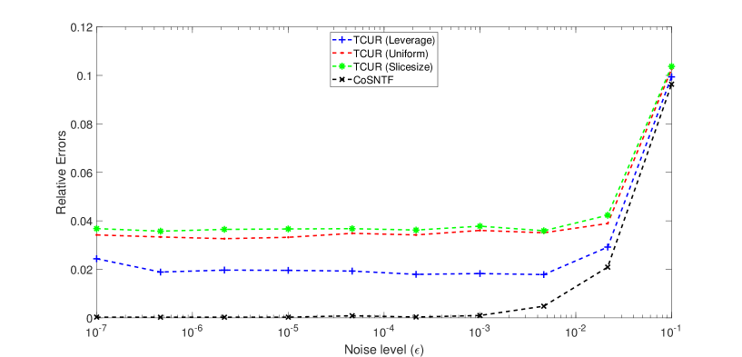
Figure 3: Average relative error on the fully randomly generated coseparable tensors.

From Figure 3, one can see our CoS-NTF index sampling achieves low relative errors, which proves its feasibility and shows its ability to accurately select indices for generating the coseparable core. Meanwhile, the TCUR index sampling shows larger relative errors across all three sampling distributions. It falls short in accurately reconstructing the coseparable tensors compared to CoS-NTF index sampling because the randomness introduces errors. Specifically, the randomly sampled indices may not satisfy the conditions of Theorem 3.9 (ii).

Then we delve into a detailed analysis of the TCUR index sampling. Since the tensor $\mathcal{A}$ is generated from the uniform distribution, each slice will have nearly the same sampling probability for the slice-size sampling, resulting in a similar result with the uniform sampling. We can also see that the leverage sampling performs slightly better because it gives more sampling weights to rows or columns with more information than the other two sampling distributions.

5.2 Facial data sets

In this section, we apply our proposed CoS-NTF and TCUR index selection algorithms on facial data sets to test their clustering abilities. The data sets we used are briefly described as follows.

• The Extended Yale Face Database B (YaleB) [11] contains 2414 grayscale images from 38 distinct individuals captured under 64 different lighting conditions. Each image has an original size of $192\times 168$ pixels, which we subsequently resize to $24\times 21$ pixels. We also selected 20 face images for each individual at random to obtain 760 images. Since the same individuals can be regarded as the same cluster and $r_{2}$ represents the clustering number, we set $r_{2}=38$. $r_{1}=24$ is set to be the row number of the resized images.

• The ORL Database of Faces (ORL) [30] contains 400 grayscale images from 40 distinct subjects, where each subject has ten different images taken at different lighting, facial expressions, and facial details. The size of each image is $112\times 92$ pixels and we resize them to $23\times 19$ pixels. We set $r_{1}=23$, $r_{2}=40$.

• The Frey Face Dataset (Frey) is collected by Brendan Frey, which contains 1965 grayscale images of Brendan Frey’s face, taken from sequential frames of a small video. The size of each image is $20\times 28$, so we set $r_{1}=r_{2}=20$.

• The MIT-CBCL Face Database #1 (CBCL) [21] consists of a training set of 2429 grayscale face images and a test set of 472 face images of size $19\times 19$ pixels. We take the training data set and set $r_{1}=19$ and $r_{2}=49$ as in [25].

• The UMIST Face Database (UMist) [16] consists of 575 grayscale face images of 20 different people. Each image has $112\times 92$ size and we resize them into $28\times 23$ pixels. We set $r_{1}=r_{2}=20$.

For each dataset, we arrange all the images into a tensor $\mathcal{A}\in\mathbb{R}_{+}^{m\times n\times p}$, where $m$ and $p$ stand for the size of the image and $n$ is the number of images. For example, $\mathcal{A}^{\mathrm{YaleB}}\in\mathbb{R}_{+}^{24\times 760\times 21}$, $\mathcal{A}^{\mathrm{ORL}}\in\mathbb{R}_{+}^{23\times 400\times 19}$.

Note that some matrix index selection methods can also be used to cluster the facial data sets, including the Coseparable NMF method, where they vectorize each image and arrange them into a matrix, like ${A}^{\mathrm{YaleB}}\in\mathbb{R}_{+}^{\left(24\times 21\right)\times 760}$ and ${A}^{\mathrm{ORL}}\in\mathbb{R}_{+}^{\left(23\times 19\right)\times 400}$ for the data sets above. We also compare our methods with these state-of-the-art index selection methods. We first summarize them as follows.

• The Successive Projections Algorithm (SPA) [9] is a forward method to select the column of the matrix $A$ with the largest $l_{2}$ norm and then calculate the projections of all columns on the orthogonal complement of the selected column at each step. We will apply SPA on $A$ and $A^{\top}$ to select $r_{2}$ columns and $r_{1}$ rows of $A$ respectively. We call it SPA+ method.

• The Coseparable NMF Fast Gradient Method (CoS-NMF) is an alternating fast gradient method to solve the coseparable NMF problem proposed in [29] and determine the rows and columns of the coseparable core. We follow the same settings as [29], i.e., $\delta=10^{-2}$, $maxiter=1000$ and using the simplest postprocessing to select $r_{1}$ rows and $r_{2}$ columns in the SNMF-FGM step. The regularization parameter $\lambda$ is fixed at 0.25 after experimenting with values ranging from $10^{-3}$ to $1$.

• The Matrix CUR sampling (CUR) is a randomized sampling method to select rows and columns for the CUR decomposition factor, the submatrix $U$. Its sampling stability and complexity have been proved in [17]. Similar to our TCUR index sampling, we will uniformly sample $r_{1}\log(m)$ rows and $r_{2}\log(n)$ columns from the $m\times n$ original data matrix, and then use matrix DEIM [6] to enforce the sampled submatrix to be $r_{1}\times r_{2}$.

As our CoS-NTF method can directly handle the facial data as a whole, it needs additional $\mathsf{unfold}$ operations in each step. Moreover, the unfolded matrix may have a highly imbalanced row-column ratio, resulting in a significant increase in runtime. However, we have proved the relationship between the t-CUR decomposition and coseparable NTF, as well as the t-CUR sampling theory. Motivated by these findings, we adopt a hybrid approach: first pre-selecting indices randomly, such as $r_{1}\log(m)$ horizontal slices and $r_{2}\log(n)$ lateral slices, and then applying the CoS-NTF index selection on this pre-selected subtensor. This strategy effectively reduces runtime.

After selecting the row and column indices $\tilde{\mathbf{I}},\tilde{\mathbf{J}}$, we adopt the [29, Algorithm 3] to compute their nonnegative factors $\tilde{P}_{1},\tilde{P}_{2}$ and reconstruct the approximate solutions $\tilde{A}=\tilde{P}_{1}A_{\tilde{\mathbf{I}}\tilde{\mathbf{J}}}\tilde{P}_{2}$ for the three matrix methods. For our TCUR and CoS-NTF methods, we compute the tensors $\widetilde{\mathcal{P}}_{1}$ and $\widetilde{\mathcal{P}}_{2}$ by the Algorithm 6 and reach the approximate solutions $\widetilde{\mathcal{A}}=\widetilde{\mathcal{P}}_{1}\ast\mathcal{A}_{\mathbf{\widetilde{I}\widetilde{J}}:}\ast\widetilde{\mathcal{P}}_{2}$ as section 5.1. In Table 1, we show the relative approximations (in percent)

$$1-\frac{\left\|{A}-\tilde{A}\right\|_{\mathrm{F}}}{\left\|{A}\right\|_{\mathrm{F}}},\quad 1-\frac{\left\|\mathcal{A}-\widetilde{\mathcal{A}}\right\|_{\mathrm{F}}}{\left\|\mathcal{A}\right\|_{\mathrm{F}}}.$$

Table 1: Relative approximations for the facial datasets.

Database	$\left(r_{1},r_{2}\right)$	CoS-NTF	TCUR	SPA+	CoS-NMF	CUR
YaleB	$\left(24,38\right)$	77.1951	78.8222	76.9635	73.3576	76.1316
ORL	$\left(23,40\right)$	84.5293	85.1224	81.5256	80.2834	81.8961
Frey	$\left(20,20\right)$	88.9242	89.1692	88.5569	86.4034	88.5093
CBCL	$\left(19,49\right)$	82.4520	82.3346	80.4568	79.5455	79.8641
UMist	$\left(20,20\right)$	75.2229	78.1479	75.0243	73.2131	74.5673

Table 1 shows that our CoS-NTF and TCUR methods have higher relative approximation on all 5 databases, which indicates they perform better in clustering than the matrix methods. It also demonstrates that handling the high dimensional data directly and keeping their high-order structure can better retain the original information.

Besides, the TCUR method performs slightly better than the CoS-NTF method. And since TCUR sampling is a randomized method and the CoS-NTF method needs to run the fast gradient method iteratively, the TCUR method runs faster, which shows the potential of our proposed TCUR sampling theory.

Furthermore, the matrix CUR sampling method also performs well among the three matrix methods. It is an efficient way to sample row/column indices for the matrix.

6 Conclusion

In this paper, we extend the concept of coseparability to tensors under the t-product framework and propose coseparable NTF. For this factorization, we investigate its characterizations and its relationship with t-CUR decomposition. Using the SNMF-FGM algorithm, we also introduce an algorithm to alternately select the coseparable indices. Additionally, based on t-CUR decomposition, we propose the t-CUR sampling theory and combine it with the t-DEIM method to establish another random algorithm, the TCUR-DEIM algorithm, for selecting coseparable indices. Then for the selected coseparable cores, we need to solve alternating tensor least squares problems to obtain the nonnegative factors. Therefore, we use the definition of the t-product to unfold the tensor and solve the corresponding matrix least squares problems.

For the proposed TCUR and CoS-NTF methods, we first test them with synthetic coseparable tensors. The result shows that the CoS-NTF method effectively selects coseparable indices, and the TCUR method has relatively larger errors due to its randomness, where the leverage score sampling can assign more sampling weights to slices with more information, and outperforms uniform sampling and slice-size sampling. Furthermore, on the real facial data sets, we compare their clustering abilities with three matrix sampling methods. The results suggest that our TCUR and CoS-NTF methods require more runtime since they should unfold tensors and the unfolded tensors have an unbalanced row-column ratio in each iterative computation. Due to our methods processing each image as a whole rather than vectorizing it, they can retain more original information compared to the three matrix methods, which results in higher relative approximations. It shows the potential of the proposed tensor methods for handling high-dimensional data.

References

- [1] S. Ahmadi-Asl, A.-H. Phan, C. F. Caiafa, and A. Cichocki, Robust low-tubal-rank tensor recovery using discrete empirical interpolation method with optimized slice/feature selection, ArXiv, abs/2305.00749 (2023).
- [2] S. Arora, R. Ge, Y. Halpern, D. Mimno, A. Moitra, D. Sontag, Y. Wu, and M. Zhu, A practical algorithm for topic modeling with provable guarantees, in Proceedings of the 30th International Conference on Machine Learning, vol. 28, Atlanta, Georgia, USA, 17–19 Jun 2013, PMLR, pp. 280–288.
- [3] R. Behera, J. K. Sahoo, R. N. Mohapatra, and M. Z. Nashed, Computation of generalized inverses of tensors via t-product, Numerical Linear Algebra with Applications, 29 (2022), p. e2416.
- [4] I. Buciu, Non-negative matrix factorization, a new tool for feature extraction: theory and applications, International Journal of Computers, Communications and Control, 3 (2008), pp. 67–74.
- [5] H. Cai, K. Hamm, L. Huang, J. Li, and T. Wang, Rapid robust principal component analysis: CUR accelerated inexact low rank estimation, IEEE Signal Processing Letters, 28 (2020), pp. 116–120.
- [6] S. Chaturantabut and D. C. Sorensen, Nonlinear model reduction via discrete empirical interpolation, SIAM Journal on Scientific Computing, 32 (2010), pp. 2737–2764.
- [7] J. Chen, W. Ma, Y. Miao, and Y. Wei, Perturbations of Tensor-Schur decomposition and its applications to multilinear control systems and facial recognitions, Neurocomputing, 547 (2023). 126359.
- [8] J. Chen, Y. Wei, and Y. Xu, Tensor CUR decomposition under T-product and its perturbation, Numerical Functional Analysis and Optimization, 43 (2022), pp. 698–722.
- [9] M. C. U. de Araújo, T. C. B. Saldanha, R. K. H. Galvão, T. Yoneyama, H. C. Chame, and V. Visani, The successive projections algorithm for variable selection in spectroscopic multicomponent analysis, Chemometrics and Intelligent Laboratory Systems, 57 (2001), pp. 65–73.
- [10] D. Donoho and V. Stodden, When does non-negative matrix factorization give a correct decomposition into parts?, in Proceedings of the 16th International Conference on Neural Information Processing Systems, NIPS’03, Cambridge, MA, USA, 2003, MIT Press, p. 1141–1148.
- [11] A. S. Georghiades, P. N. Belhumeur, and D. J. Kriegman, From few to many: Illumination cone models for face recognition under variable lighting and pose, IEEE Trans. Pattern Anal. Mach. Intell., 23 (2001), pp. 643–660.
- [12] N. Gillis, Successive nonnegative projection algorithm for robust nonnegative blind source separation, SIAM Journal on Imaging Sciences, 7 (2014), pp. 1420–1450.
- [13] N. Gillis and F. Glineur, Accelerated multiplicative updates and hierarchical ALS algorithms for nonnegative matrix factorization, Neural computation, 24 (2012), pp. 1085–1105.
- [14] N. Gillis and R. Luce, A fast gradient method for nonnegative sparse regression with self-dictionary, IEEE Transactions on Image Processing, 27 (2018), pp. 24–37.
- [15] N. Gillis and S. A. Vavasis, Fast and robust recursive algorithmsfor separable nonnegative matrix factorization, IEEE Transactions on Pattern Analysis and Machine Intelligence, 36 (2014), pp. 698–714.
- [16] D. B. Graham and N. M. Allinson, Characterising Virtual Eigensignatures for General Purpose Face Recognition, Springer Berlin Heidelberg, Berlin, Heidelberg, 1998, pp. 446–456.
- [17] K. Hamm and L. Huang, Perspectives on CUR decompositions, Applied and Computational Harmonic Analysis, 48 (2020), pp. 1088–1099.
- [18] F. Han, Y. Miao, Z. Sun, and Y. Wei, T-ADAF: Adaptive data augmentation framework for image classification network based on tensor T-product operator, Neural Processing Letters, 55 (2023), pp. 10993 – 11016.
- [19] N. Hao, L. Horesh, and M. E. Kilmer, Nonnegative Tensor Decomposition, Springer Berlin Heidelberg, Berlin, Heidelberg, 2014, pp. 123–148.
- [20] R. A. Harshman, Foundations of the PARAFAC procedure: Models and conditions for an ”explanatory” multi-modal factor analysis, UCLA Working Papers in Phonetics, 16 (1970), pp. 1–84.
- [21] J. Huang, B. Heisele, and V. Blanz, Component-based face recognition with 3D morphable models, 2004 Conference on Computer Vision and Pattern Recognition Workshop, (2003), pp. 85–85.
- [22] M. E. Kilmer and C. D. M. Martin, Factorization strategies for third-order tensors, Linear Algebra and its Applications, 435 (2011), pp. 641–658.
- [23] T. G. Kolda and B. W. Bader, Tensor decompositions and applications, SIAM Rev., 51 (2009), pp. 455–500.
- [24] D. Kuang, J. Choo, and H. Park, Nonnegative matrix factorization for interactive topic modeling and document clustering, Partitional clustering algorithms, (2015), pp. 215–243.
- [25] D. D. Lee and H. S. Seung, Learning the parts of objects by non-negative matrix factorization, Nature, 401 (1999), pp. 788–791.
- [26] M. W. Mahoney and P. Drineas, CUR matrix decompositions for improved data analysis, Proceedings of the National Academy of Sciences, 106 (2009), pp. 697 – 702.
- [27] Y. Miao, L. Qi, and Y. Wei, T-Jordan canonical form and T-Drazin inverse based on the T-product, Communications on Applied Mathematics and Computation, 3 (2020), pp. 201 – 220.
- [28] I. Oseledets, Tensor-train decomposition, SIAM Journal on Scientific Computing, 33 (2011), pp. 2295–2317.
- [29] J. Pan and M. K. Ng, Coseparable nonnegative matrix factorization, SIAM Journal on Matrix Analysis and Applications, 44 (2023), pp. 1393–1420.
- [30] F. Samaria and A. Harter, Parameterisation of a stochastic model for human face identification, Proceedings of 1994 IEEE Workshop on Applications of Computer Vision, (1994), pp. 138–142.
- [31] S. Soltani, M. E. Kilmer, and P. C. Hansen, A tensor-based dictionary learning approach to tomographic image reconstruction, BIT Numerical Mathematics, 56 (2015), pp. 1425 – 1454.
- [32] D. A. Tarzanagh and G. Michailidis, Fast randomized algorithms for t-product based tensor operations and decompositions with applications to imaging data, SIAM Journal on Imaging Sciences, 11 (2018), pp. 2629–2664.
- [33] L. R. Tucker, Some mathematical notes on three-mode factor analysis, Psychometrika, 31 (1966), pp. 279–311.
- [34] W. Xu, X. Liu, and Y. Gong, Document clustering based on non-negative matrix factorization, in Proceedings of the 26th annual international ACM SIGIR conference on Research and development in informaion retrieval, 2003, pp. 267–273.
- [35] Z. Zhang, G. Ely, S. Aeron, N. Hao, and M. Kilmer, Novel methods for multilinear data completion and de-noising based on Tensor-SVD, in 2014 IEEE Conference on Computer Vision and Pattern Recognition, 2014, pp. 3842–3849.
- [36] Q. Zhao, G. Zhou, S. Xie, L. Zhang, and A. Cichocki, Tensor ring decomposition, ArXiv, abs/1606.05535 (2016).
- [37] Y. Zhu and Y. Wei, Tensor LU and QR decompositions and their randomized algorithms, Computational Mathematics and Computer Modeling with Applications (CMCMA), (2022).