Localizing uniformly moving mono-frequent sources using an inverse 2.5D approach

Abstract

Localizing linearly moving sound sources using microphone arrays is particularly challenging as the transient nature of the signal leads to relatively short observation periods. Commonly, a moving focus is used and most methods operate at least partially in the time domain. In contrast, here an inverse source localization algorithm for mono-frequent uniformly moving sources that acts entirely in the frequency domain is presented. For this, a 2.5D approach is utilized and a transfer function between sources and a microphone grid is derived. By solving a least squares problem using the data at the microphone grid, the unknown source distribution in the moving frame can be determined. For that the measured time signals need to be transformed into the frequency domain using a windowed discrete Fourier transform (DFT), which leads to effects such as spectral leakage that depends on the length of the time interval and the analysis window used.

To include these effects in the numerical model, the calculation of the transfer matrix is modified using the Fourier transform of the analysis window. Currently, this approach is limited to mono-frequent sources as this allows a simplification of the calculation and reduces the computational effort. The least squares problem is solved using a Tikhonov regularization employing an L-curve approach to determine a suitable regularization parameter. As a moving source is considered, the Doppler effect allows to enhance the stability of the system by combining the transfer functions for multiple frequencies in the measured signals. The performance of the approach is validated using simulated data of a moving point source with or without a reflecting ground. Numerical experiments are performed to show the effect of the choice of frequencies in the receiver spectrum, the effect of the DFT, the frequency of the source, and the distance of source and receiver.

[ARI]organization=Acoustics Research Institute, Austrian Academy of Sciences, addressline=Dominikanerbastei 16, city=Vienna, postcode=A-1010, country=Austria

1 Introduction

The localization of sound sources is an important topic in order to efficiently reduce noise burden in the environment. Microphone arrays are one of the major tools used for sound source localization. By far the most popular method of choice is beamforming and all its flavors (see, e.g., [4, 25] for extensive reviews on the topic).

Briefly, beamforming methods virtually focus the microphone array on a potential source position, suppressing signals coming from other locations. In general, these methods are based on the assumption of free field wave propagation. In stationary conventional beamforming, where non-moving source are assumed, the cross-spectral matrix of the microphone signals is calculated as well as the so-called steering vector. The steering vector determines the focus of the beamforming algorithm based on the known propagation of the signal from the respective source position to the microphone positions. Using all points of a predefined source grid as focus points, a beamforming map is generated. The so produced raw beamforming map usually is subject to a point-spread-function, i.e., the beamforming map of a point source is blurred and subject to sidelobes depending on different factors such as the frequency, array geometry, as well as distance between the array and source grid. To produce a better resolved source map, deconvolution approaches such as DAMAS (deconvolution approach for the mapping of acoustic sources, [3, 9]) or CLEAN-SC [33] are applied to the beamforming results. For a comparison of different deconvolution methods see, e.g., [18] and for more details on beamforming in general please refer to, e.g., [4, 25].

For moving sources, the typical approach is to use a moving focus, i.e., a steering vector which is altered over time. In [13], a frequency domain approach was developed, where short time windows are used to limit the source displacement and allow for an approximate Doppler compensation. Various deconvolution approaches were then combined with this spectral beamforming approach. Methods which are at least partially located in the time domain are used more commonly for moving sources (cf. [7, 15, 32, 38, 39]). These methods use a time domain formulation for the pressure caused by a moving point source and thus take the Doppler shift into account. In contrast to the frequency domain approach in [13], no assumptions about small displacements are necessary. However, in the time domain the propagation path must typically be calculated for very high number of time points. While the method of [7] (including the deconvolution approach CLEANT) works fully in the time domain, many approaches apply frequency domain methods after some initial time domain processing steps (e.g. [15, 32, 38, 39]). Importantly, the present work is solely concerned with linearly moving sources. Other types of motion may require other approaches, see e.g. [6, 14] for rotating fans.

Irrespective of whether time or frequency domain is used or which type of deconvolution approach is applied, the aforementioned methods and its many variants are based on conventional beamforming, i.e., focusing the array using a steering vector. A different idea is used in so-called inverse schemes. In conventional beamforming the strength of each source is determined independently of the others. Only the deconvolution step, which also solves an inverse problem, considers the dependencies within this raw beamforming map. In contrast, inverse methods exist, where a joint optimization problem is solved directly on the measurements. The remainder of this manuscript is concerned with this latter class of methods. Although, these inverse methods can of course be applied to the free-field wave propagation (e.g., generalized inverse beamforming [34], spectral estimation methods [2, 37, 18] and extensions thereof [27], compressive beamforming [24]), the inverse approach allows for a much more general definition of sources and the surrounding environment. Using numerical approaches like the boundary element method (BEM) or the finite element method (FEM), scattering structures and other types of sources such as velocity elements can be included in the forward model (e.g., [14, 31]) which is not or only to a limited degree possible in conventional beamforming (including deconvolution). This is, e.g., important when significant ground reflections affect the measurements or in confined spaces when reflecting objects are in the vicinity (e.g. [14]). Note that for the case of point sources over a fully reflecting ground, a conventional beamforming approach was also developed [5] which was later extended to include a deconvolution step [40].

Although computationally demanding, the forward problem is often comparatively straight forward for stationary sources. However, the inversion of the forward map poses some difficulties. As there are, in general, more potential source positions than receiver points (i.e., microphones), the transfer map/matrix from source to array is underdetermined. Many different approaches exist to address this problem, and the way the inverse problem is regularized allows to control properties of the solution such as smoothness or sparseness. For example, in [31], a standard Tikhonov regularization (a small squared $L_{2}$ norm of the unknown source strengths is used as additional condition) was used to stabilize the inversion which led to typically smooth source maps. To find a suitable regularization parameter, the L-curve approach was applied where a range of regularization parameters is used to solve the problem and from these results the degree of regularization is determined that “best” represents a compromise between model error and regularization (for details see e.g., [17]). If it can be assumed that only few localized source points have non-zero strengths, sparse methods, that, e.g., minimize the $L_{1}$-norm of the solution instead of the $L_{2}$-norm, can be used (cf. generalized inverse beamforming, [34]). Recently, an inverse scheme based on FEM for stationary sources was introduced [14] where a norm was used on the source map coefficients with a non-integer exponent lying between 1 and 2. When setting the value close to 1, some sparsity can be enforced. Another example is given in [24], where a compressive beamforming approach (i.e., inverse beamforming using an $L_{1}$-regularization) is introduced for linearly moving sources which operates entirely in the time domain. There, the forward problem is set up for time points in a pre-defined period and then the full system is solved. These are only but a few methods to find regularized solutions to linear systems of equations.

In the present work, an inverse approach for sound source localization of mono-frequent sources moving at a constant speed is presented that operates fully in the frequency domain. The effect of the motion of the source is incorporated in closed form in the forward transfer function using a 2.5D approach based on the Helmholtz equation. This allows for the consideration of, in theory, arbitrarily long time windows without the necessity of dividing the observations into shorter segments. In the 2.5D approach a constant cross-section in the $y$-$z$ plane is assumed, but in contrast to pure 2D methods the sound field may vary along $x$ allowing for the modeling of point sources, incoherent line sources, or sources of finite length. This is achieved by employing a spatial Fourier transform along $x$ to transform the Helmholtz equation into the wavenumber domain. The 3D sound field is calculated by solving a number of 2D problems with different wavenumbers and an inverse Fourier transform is used to get back to the spatial domain in $x$ (see e.g., [10, 12, 19, 21, 22, 23, 29, 36]). The 2.5D BEM also allows for a straight-forward definition of impedance boundary conditions [11]. Thus, the Helmholtz BEM including its 2.5D variant is a very versatile and established tool in noise research.

Although, a major advantage of the 2.5D approach is that sources moving along $x$ at a constant speed $v_{s}$ can be treated in a straightforward manner in this setting (for a derivation see, e.g., [10]), the main problem of this approach is that the measured signals at the microphone array and the numerically calculated transfer matrix, which consists of the transfer functions from source to the receiver points, are defined in different domains. Thus, the first step is to transform them into a common domain, which is in our approach given by the frequency domain.

Unfortunately, while the transfer functions and hence the transfer matrix used for the inversion are described using continuous Fourier integral transforms, the measured data can only be transformed using a discrete Fourier transform (DFT). This transformation results in undesirable effects, most notably spectral leakage from adjacent frequency bands which is dependent on the length of the observation period and the possible use of an analysis window before the DFT. While the choice of the latter allows some control over the leakage, increasing the observation period is very limited in the case of linearly moving sources, because pass-by events are, in general, very brief. As a consequence, even though the transfer function and the measurements after applying the DFT are both in the frequency domain, there is a substantial difference between the two entities. The novelty in the approach presented is to include the effects of the DFT in the calculation of the final transfer matrix, thus bringing it to the same discrete frequency domain as the measurements. The inversion of this transfer matrix is done using a Tikhonov regularization and the regularization factor is determined using the L-curve approach [16]. To stabilize the L-curve a small amount of uncorrelated noise was used as suggested in [20]. This basic approach is chosen because the focus of the present work is to investigate the general mapping properties of the matrix w.r.t. to the achievable resolution for point sources. Finding potentially better suited inversion routines based , e.g., on compressive sensing techniques, are beyond the focus of this manuscript. Also, to allow for a simplification of the calculation and reduction in the computational effort the algorithm is currently limited to mono-frequent sources.

The newly developed algorithm was thoroughly tested using simulated data comprising moving mono-frequent point sources in the free-field without and with a reflecting half-plane to model reflections from the ground. The test data was generated using a time domain approach (cf. [8]). A state-of-the-art array geometry based on a spiral arrangement was used to define the microphone positions. The effect of different parameters such as source frequency, analysis window length, and choice of observed frequencies was investigated.

This paper is structured as follows. First a detailed derivation of the algorithm is provided in Sec. 2. Note that although the test cases comprise only moving point sources, the derivation is in principle valid for general 2.5D boundary equation models. After a detailed overview of the simulated test cases the results on the method’s performance under different settings are provided in Sec. 3. A summary and concluding remarks are provided in Sec. 4.

2 Methods

2.1 Transfer function in 2.5D

The 2.5D approach was developed to efficiently calculate scattering from very long structures in 3D for stationary as well as for uniformly moving sources [10]. In this section, a concise introduction to this method is given to keep the manuscript self contained.

If the scattering object is infinitely long along one direction and has a constant cross-section (in practice this is, e.g., approximately true for a long noise barrier), the 2.5D approach can be used to reduce a full 3D acoustic scattering problem into a series of 2D problems with different wavenumbers. For the remainder of this manuscript the infinite dimension, which is also the direction of motion, is defined along the $x$-axis, while the 2D cross-section is in the $y$-$z$-plane.

Briefly, the general 2.5D approach is based on a Fourier transform $x\xrightarrow{\mathcal{F}}k_{x}$ (cf. [10, 12, 19, 22, 23, 29, 36]), where $k_{x}$ is the wavenumber with respect to the $x$-axis. With this transformation, the Green’s function for the Helmholtz equation in 3D can be represented by

$$\frac{\mathrm{e}^{\mathrm{i}kr_{3}}}{4\pi r_{3}} =\frac{1}{2\pi}\int\limits_{-\infty}^{\infty}\frac{\mathrm{i}}{4}\mathrm{H}_{0}\!\left(r_{2}\sqrt{\omega^{2}/c^{2}-k^{2}_{x}}\right)\mathrm{e}^{\mathrm{i}k_{x}(x_{r}-x_{s})}dk_{x},$$ (1)

where ${\bf x}_{s}=\left(x_{s},y_{s},z_{s}\right)^{\top}$ and ${\bf x}_{r}=\left(x_{r},y_{r},z_{r}\right)^{\top}$ are a given source and receiver point in 3D, respectively. $r_{2}=\sqrt{(y_{r}-y_{s})^{2}+(z_{r}-z_{s})^{2}}$ is defined as the Euclidean distance in the $y$-$z$-plane between these points and $r_{3}=||{\bf x}_{r}-{\bf x}_{s}||_{2}$ gives their distance in 3D. $\mathrm{H}_{0}\!\left(\cdot\right)$ denotes the Hankel-function of the first kind of order 0 (the Green’s function for the 2D Helmholtz equation), $k=\omega c^{-1}$, where $\omega$ is the angular frequency of interest for the 3D problem and $c$ denotes the speed of sound. In short, the 3D Green’s function with wavenumber $k=\omega c^{-1}$ can be represented by an integral with respect to $k_{x}$ (inverse Fourier transform) over 2D Green’s functions with 2D wavenumbers $k_{2}=\sqrt{\omega^{2}/c^{2}-k_{x}^{2}}$. $k_{x}$ denotes the (spatial) wavenumber along the $x$-dimension.

More generally, this approach can be combined with the boundary element method (BEM) to include (infinitely long) scatterers with constant cross-sections in the $y$-$z$ plane (for a derivation see e.g. [10]). In this case, the sound pressure at a point ${\bf x}_{r}$ in 3D can be calculated as an inverse Fourier transform:

$$\hat{p}\left(x_{s},y_{s},z_{s},x_{r},y_{r},z_{r},\omega\right) =\frac{1}{2\pi}\int\limits_{-\infty}^{\infty}\hat{q}\!\left(y_{s},z_{s},y_{r},z_{r},\sqrt{\omega^{2}/c^{2}-k^{2}_{x}}\right)\mathrm{e}^{\mathrm{i}k_{x}(x_{r}-x_{s})}dk_{x},$$ (2)

with $\hat{q}\!\left(\cdot\right)$ being the 2D BEM solution at the receiver point in the $y$-$z$-plane for a source located at $\left(y_{s},z_{s}\right)^{\top}$ and a 2D wavenumber $k_{2}=\sqrt{\omega^{2}/c^{2}-k^{2}_{x}}$. $x_{r}-x_{s}$ simply denotes the offset of the receiver w.r.t. the source position along the $x$-dimension. Importantly, the term source does not imply a specific source type and could be an external point source but also velocity or pressure boundary conditions as long as their Fourier transform with respect to $x$ exists. For details on the definition of velocity boundary conditions in the 2.5D BEM see [23]. In addition to different source types the 2.5D BEM can also include admittance boundary conditions and absorbing grounds [11]. Eq. (2) can also be defined for multiple concurrent sources, however, if the sources have different $x$-offsets, their respective contributions to $\hat{q}\!\left(\cdot\right)$ either have to be weighted with the appropriate phase factor resulting from the spatial shift or calculated separately and then added.

For the simplest case of a single point source at ${\bf x}_{s}=(x_{s},y_{s},z_{s})^{\top}$ and no scattering objects, the 2D solution is simply $\hat{q}\!\left(y_{s},z_{s},y_{r},z_{r},k_{2}\right)=\frac{\mathrm{i}}{4}\mathrm{H}_{0}\!\left(r_{2}k_{2}\right)$ as in Eq. (1).

To numerically calculate the inverse Fourier transform, the integral in Eq. (2) is replaced by a quadrature formula, e.g., Gauss-type quadrature ([10, 36]) or a Filon-Clenshaw-Curtis quadrature [22]. For every quadrature node one 2D calculation needs to be performed.

2.1.1 Source-receiver relation for a uniformly moving source

Eq. (2) is only valid for stationary sources. The time-dependent pressure caused by a uniformly moving point source, which is the case investigated here, was derived previously [10, 29]. Briefly, a single point source emitting a source signal $s(t)$ in the time domain is assumed which moves at a constant speed of $v_{s}$ along $x$: $x_{s}(t)=x_{0}+v_{s}t$. The pressure at the receiver position $\left(x_{r},y_{r},z_{r}\right)^{\top}$ at time $t$ is given as:

$$p(x_{0},y_{s},z_{s},x_{r},y_{r},z_{r},t) =\frac{1}{(2\pi)^{2}}\int\limits_{-\infty}^{\infty}\!\int\limits_{-\infty}^{\infty}\hat{s}(\omega-v_{s}k_{x})\hat{q}\!\left(y_{s},z_{s},y_{r},z_{r},\sqrt{\omega^{2}/c^{2}-k^{2}_{x}}\right)\mathrm{e}^{\mathrm{i}k_{x}(x_{r}-x_{0})}\mathrm{e}^{-i\omega t}dk_{x}d\omega.$$ (3)

$\hat{s}(\omega-v_{s}k_{x})$ is the Fourier transform of $s(t)$ evaluated at $\omega-v_{s}k_{x}$. In contrast to Eq. (2), Eq. (3) defines the pressure at the receiver point ${\bf x}_{r}$ in the time domain. This definition in the time domain provides the basis for incorporating the effects of the discrete Fourier transform (DFT) into the transfer matrix.

A general source localization scenario is defined by a (possibly moving) source region containing $L$ potential (point) sources at positions ${\bf x}_{s,\ell},\ell=1,\dots,L$ and a microphone array with $N$ microphones at positions ${\bf x}_{r,n},n=1,\dots,N$, and typically $N<L$. In case of a moving point source along the $x$-axis, the first component $x_{s,\ell}$ of ${\bf x}_{s,\ell}$ denotes the $x$-coordinate for the source at time $t=0$ s. To simplify the notation in Eq. (3), the pressure at ${\bf x}_{r,n}$ caused by a source at ${\bf x}_{s,\ell}$ will be denoted by $p_{n\ell}(t)$ leading to the time domain formulation

$$p_{n\ell}(t) =\frac{1}{(2\pi)^{2}}\int\limits_{-\infty}^{\infty}\!\int\limits_{-\infty}^{\infty}\hat{s}_{\ell}(\omega-v_{s}k_{x})\hat{q}_{\ell n}\!\left(\sqrt{\omega^{2}/c^{2}-k^{2}_{x}}\right)\mathrm{e}^{\mathrm{i}k_{x}(x_{r,n}-x_{s,\ell})}\mathrm{e}^{-\mathrm{i}\omega t}dk_{x}d\omega$$ (4)

and the continuous frequency domain formulation

$$\hat{p}_{n\ell}(\omega)=\frac{1}{2\pi}\int\limits_{-\infty}^{\infty}\hat{s}_{\ell}(\omega-v_{s}k_{x})\hat{q}_{\ell n}\!\left(\sqrt{\omega^{2}/c^{2}-k^{2}_{x}}\right)\mathrm{e}^{\mathrm{i}k_{x}(x_{r,n}-x_{s,\ell})}dk_{x}$$ (5)

This equation is valid for any arrangement of sources and receivers.

In an ideal, continuous setting, Eq. (5) would act as the starting point of the inverse method, as it provides a transfer function between any source point ${\bf x}_{s,\ell}$ and any receiver point ${\bf x}_{r,n}$ that can be used to compare the calculated field at the receiver with microphone array measurement at the same position. From this, the unknown source spectra $\hat{s_{\ell}}$ could, in theory, be derived. In practice, however, Eq. (5) cannot be directly applied and the discrete nature of the measurements and restrictions of the source spectra need to be considered.

2.2 Discrete Domain Formulation

The measurements using a microphone array are discrete in space as well as in time. Due to the limited number of microphones and the practical sizes of microphone arrays, a Fourier transformation of the measured data from the spatial $x$-domain into $k_{x}$ is not feasible and will thus not be considered.

The discrete Fourier transform (DFT) required to transform the measured sampled data from the time to the frequency domain is also not ideal since, in the case of linear motion, the observation time is strongly limited. Depending on the noise level and the duration (and thus the speed of the pass-by of the moving source) the signal of interest will eventually disappear in the noisy background at some point and extending the time any further will increase the noise level of the measurement without gaining any additional information. Limiting the observation time leads to two effects for the DFT: First, the frequency resolution decreases for shorter observation periods, and, secondly, spectral leakage effects increase (i.e., the observed spectral level at a given frequency contains also energy from adjacent frequencies). While zero padding (sinc-interpolation in $\omega$) can artificially improve the spectral resolution, the leakage effects are not affected and a direct comparison to the continuously transformed coefficients $\hat{p}_{n\ell}$ from Eq. (5) may turn out to be problematic. This leads to the main idea of transforming Eq. (4) to include the same effects of the DFT in time used for the measurements. In the next Section the approach of how the DFT is applied efficiently to Eq. (4) without actually calculating $p_{n\ell}(t)$ will be described.

2.2.1 Discrete Fourier transformation of the transfer function

For deriving the pressure $p(t)$ in Eqs. (4) and (5) the (continuous) Fourier transform is used:

$$\hat{p}(\omega) =\mathcal{F}(p)(\omega)=\int\limits_{-\infty}^{\infty}p(t)\mathrm{e}^{\mathrm{i}\omega t}dt,$$ (6)

$$p(t) =\mathcal{F}^{-1}(\hat{p})(t)=\frac{1}{2\pi}\int\limits_{-\infty}^{\infty}\hat{p}\left(\omega\right)\mathrm{e}^{-\mathrm{i}\omega t}d\omega.$$ (7)

To avoid a cluttered notation, the indices indicating source and receiver have been dropped.

Sampling the continuous pressure signal $p(t)$ with a sampling time of $T_{s}=f_{s}^{-1}$ (time difference between samples or inverse of the sampling frequency) and applying an analysis window function $g$ with finite length $\text{supp}(g)\subseteq[0,T_{g})$ with $T_{g}=N_{g}T_{s}$, the windowed DFT for a sampled signal of $N_{g}$ samples for the $m$-th frequency bin $\omega^{\prime}_{m}$ can be written as:

$$DFT_{g}(p)[\omega^{\prime}_{m}]:=\sum\limits_{n=0}^{N_{g}-1}{p[t_{n}]}g[t_{n}]\mathrm{e}^{\mathrm{i}\omega_{m}^{\prime}t_{n}} =\frac{1}{2\pi}\int\limits_{-\infty}^{\infty}\hat{p}\left(\omega\right)\sum\limits_{n=0}^{N_{g}-1}{\!\!\mathrm{e}^{-i\omega t_{n}}g[t_{n}]\mathrm{e}^{\mathrm{i}\omega_{m}^{\prime}t_{n}}}\ d\omega$$

$$=\frac{1}{2\pi}\int\limits_{-\infty}^{\infty}\hat{p}\left(\omega\right)\sum\limits_{n=0}^{N_{g}-1}{\!\!\mathrm{e}^{\mathrm{i}t_{n}(\omega_{m}^{\prime}-\omega)}g[t_{n}]}\ d\omega,$$ (8)

where Eq. (7) was used for $p[t_{n}]$ and the order of the finite sum and the integral was exchanged. The brackets $[\cdot]$ indicate the discrete nature of the argument, $t_{n}=nT_{s}$, and $\omega_{m}^{\prime}=2\pi m\left(T_{s}N_{g}\right)^{-1}$. The frequency resolution of the DFT spectrum is thus $\Delta\!f_{\mathrm{DFT}}=f_{s}N_{g}^{-1}=T_{g}^{-1}$. Due to the finite support of $g$, the sum in Eq. (8) can be extended to $n\in\mathbb{Z}$ leading to the discrete time Fourier transform (DTFT, cf. [28]) of $g$ which is continuous in frequency and periodic with a period of $f_{s}$.

Thus, Eq. (8) can be written as:

$$DFT_{g}(p)[\omega^{\prime}_{m}]=\frac{1}{2\pi}\int\limits_{-\infty}^{\infty}\hat{p}\left(\omega\right)\sum\limits_{n=-\infty}^{\infty}{\!\!\mathrm{e}^{\mathrm{i}t_{n}(\omega_{m}^{\prime}-\omega)}g[t_{n}]}\ d\omega=\frac{1}{2\pi}\int\limits_{-\infty}^{\infty}\hat{p}\left(\omega\right)\mathcal{F}_{\text{DTFT}}(g)(\omega_{m}^{\prime}-\omega)d\omega,$$ (9)

which is simply the convolution of the Fourier transform of $p$ and the DTFT of $g$, that allows to include spectral leakage effect of the DFT into the transfer function. With this formulation the windowed DFT of the sampled version of $p(t)$ can be calculated directly from the continuous frequency domain formulation without the need of an inverse transform to the time domain.

The amount of spectral leakage depends on two factors: type and length of the window. First, the longer the window (i.e., the higher $T_{g}$) the smaller the leakage. Second, the choice of window type is crucial for the reduction of spectral leakage. When a rectangular window of length $T_{g}$ is used ($g[t_{n}]=1,\,n=0,\dots,N_{g}-1$), $\mathcal{F}_{\text{DTFT}}(g)(\omega_{m}^{\prime}-\omega)$ is the Dirichlet kernel $D_{N_{g}}\left((\omega_{m}^{\prime}-\omega)T_{s}\right)$ which resembles, loosely speaking, a periodized $\mathrm{sinc}$-function with period $2\pi$ that only slowly decays towards $\pm\pi$. For the Hanning window, e.g., the DTFT of $g[t_{n}]$ consists of the sum of three Dirichlet kernel functions which results in a faster decay of $\mathcal{F}_{\text{DTFT}}(g)$ and a considerably reduced spectral leakage which will be illustrated in the next section.

Reintroducing the subscripts $\ell$ and $n$ and plugging Eq. (5) into Eq. (9) leads to

$$\hat{p}_{n\ell}[\omega_{m}^{\prime}] :=\text{DFT}_{g}(p)[\omega_{m}^{\prime}]=\frac{1}{(2\pi)^{2}}\int\limits_{-\infty}^{\infty}\!\int\limits_{-\infty}^{\infty}\hat{s}_{\ell}(\omega-v_{s}k_{x})\hat{q}_{n\ell}\!\left(\sqrt{\omega^{2}/c^{2}-k^{2}_{x}}\right)\hat{g}(\omega_{m}^{\prime}-\omega)\mathrm{e}^{\mathrm{i}k_{x}(x_{r,n}-x_{s,\ell})}dk_{x}d\omega,$$ (10)

which is the DFT of the pressure signal given at the $n$-th receiver resulting from the $\ell$-th moving source. Note that in contrast to Eq. (5), $\hat{p}$ now denotes the windowed DFT of $p[t_{n}]$ which is indicated using brackets $[\cdot]$. $\hat{g}$ on the other hand denotes the DTFT of $g[t_{n}]$ which is continuous in frequency as indicated using parentheses.

2.2.2 Mono-frequent sources

No assumptions about $\hat{s}_{\ell}$ were used in Eq. (10). A reasonable assumption to simplify the formulation is to use a harmonic ansatz to approximate the source signal $s_{\ell}(t)$ similarly to, e.g., [14]. Thus, each source signal comprises a sum of complex exponentials

$$s_{\ell}(t)=\sum\limits_{j=1}^{J}a_{\ell j}\mathrm{e}^{-\mathrm{i}\omega_{j}t},$$ (11)

with frequencies $\omega_{j}=2\pi f_{j}$ and corresponding complex amplitudes $a_{\ell j}$.

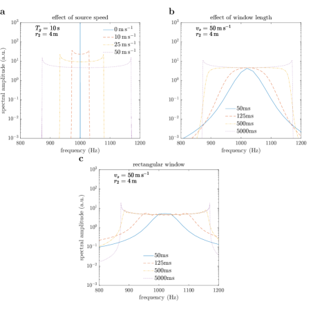
Figure 1: DFT of the signal of a moving point source at a stationary receiver. The panels show the spectral amplitudes for a mono-frequent source moving at different speeds (a), for different window lengths for a Hanning-window (b), and for a rectangular window (c). The distance between source and receiver plane was set to $r_{2}=4$ m.

In the stationary case, each frequency $f_{j}$ can be treated separately as long as the spectral leakage is adequately controlled for. If the sources are moving, each single frequency component leads to a range of observed frequencies at the stationary receivers due to the Doppler effect. This spectral range depends on the speed of the source, which in turn has an effect on the DFT and the choice of all its parameters like sampling rate, window length, and window type (see Fig. 1a to c where a source with ${f_{0}}=1000$ Hz and a source-receiver distance in the $y$-$z$-plane of $r_{2}=4$ m was used). Consequently, if the spectral ranges for different source components are overlapping, an individual treatment of the respective complex exponential is no longer possible and a joint treatment is necessary which is beyond the scope of this work. Thus, the focus of the present work will be on mono-frequent sources, i.e., a single complex exponential signal with frequency ${\omega_{0}}=2\pi f_{0}$. The source signal at the $\ell$-th source grid position ${\bf x}_{s,\ell}$ is set to $s_{\ell}(t)=a_{\ell}\mathrm{e}^{-\mathrm{i}{\omega_{0}}t}$ with the Fourier spectrum $\hat{s}_{\ell}(\omega)=a_{\ell}2\pi\delta(\omega-{\omega_{0}})$ where $\delta(\cdot)$ denotes the Dirac delta distribution.

Applying the spectrum to Eq. (10) yields

$$\hat{p}_{n\ell}[\omega_{m}^{\prime}] =\frac{a_{\ell}}{2\pi}\int\limits_{-\infty}^{\infty}\!\int\limits_{-\infty}^{\infty}\delta(\omega-v_{s}k_{x}-{\omega_{0}})\hat{q}_{n\ell}\!\left(\sqrt{\omega^{2}/c^{2}-k^{2}_{x}}\right)\hat{g}(\omega_{m}^{\prime}-\omega)\mathrm{e}^{\mathrm{i}k_{x}(x_{r,n}-x_{s,\ell})}dk_{x}d\omega$$

$$=\frac{a_{\ell}}{2\pi|v_{s}|}\int\limits_{-\infty}^{\infty}\hat{q}_{n\ell}\!\left(\sqrt{\omega^{2}/c^{2}-(\omega-{\omega_{0}})^{2}/v_{s}^{2}}\right)\hat{g}(\omega_{m}^{\prime}-\omega)\mathrm{e}^{\mathrm{i}(\omega-{\omega_{0}})v_{s}^{-1}(x_{r,n}-x_{s,\ell})}d\omega$$

$$:=h_{n\ell}[\omega^{\prime}_{m}]a_{\ell}$$ (12)

$\hat{p}_{n\ell}$ represents the (noise-free) complex sound pressure amplitude at a discrete frequency $\omega_{m}^{\prime}$ that would be “measured” at the $n$-th receiver for a mono-frequent moving source of frequency ${f_{0}}$ located at ${\bf x}_{s,\ell}=(x_{s,\ell}+vt,y_{s,\ell},z_{s,\ell})^{\top}$ when using a windowed DFT with the time window $g$. $h_{n\ell}$ is defined as the transfer function from the $\ell$-th source to the $n$-th receiver.

2.3 Numerical quadrature

It has been shown previously [22] that certain steps and special quadrature methods can be applied to numerically solve the integral in Eq. (2) efficiently. As an in-depth study of how this method can be applied to the current setting was not the focus of the work presented here, a standard adaptive quadrature was used in this manuscript using the function quadgk from MATLAB [35] which is based on a Gauss-Kronrod quadrature. A major difficulty of this inverse transformation lies in determining the integration limits which has a direct impact on the error but also on the computational effort. Every quadrature node / function evaluation implies the calculation of $\hat{q}_{n\ell}$ which, depending on the research question, may require a substantial amount of calculations.

$\hat{q}_{n\ell}$ depends on Hankel functions which have a singularity at $0$, thus, $\hat{q}_{n\ell}$ has singularities at $\omega=c\,{\omega_{0}}(c\pm v_{s})^{-1}$ which fulfill the relation $\omega^{2}/c^{2}-(\omega-\omega_{0})^{2}v_{s}^{-2}=0$. At these values the integral in Eq. (12) has to be split. For $\omega<c\,\omega_{0}\left(c+v_{s}\right)^{-1}$ or $\omega>c\,\omega_{0}\left(c-v_{s}\right)^{-1}$ Hankel functions and hence the 2D solutions $\hat{q}_{n\ell}$ decay exponentially (cf. [1], Eq. 9.2.3), thus, it is sufficient to restrict the infinite integral in Eq. (12) to a finite interval which is slightly bigger than $[c\omega_{0}\left(c+v_{s}\right)^{-1},c\omega_{0}\left(c-v_{s}\right)^{-1}]$, see for example Fig. 2, which shows the magnitude of the solution of the free-field 2D solution ($\hat{q}\!\left(\cdot\right)=H_{0}\left(\cdot\right)$) in Eq. (12) for two different source speeds (50 m s^-1: blue solid line, 25 m s^-1: orange dashed line) at $f_{0}=1000$ Hz. To illustrate the role of the window, Fig. 2 also shows $\hat{g}$ for three different time windows (gray thin lines) for a single source-receiver combination ($r_{2}=4$ m distance), and ${f_{0}}$=1000 Hz. The grey solid and dash-dotted lines show the spectra of a Hanning window for different window durations. For short time windows the Fourier transform of the window covers a wide frequency range and is only slowly decaying, thus the computational effort for the quadrature is higher. For reasons of comparison, the DTFT of a rectangular window of 1000 ms length (gray dotted thin line) is also shown, and the larger spectral leakage can be easily seen when compared to the Hanning window of the same length. The consequence at the measurement position can be seen when comparing Fig. 1b and c.

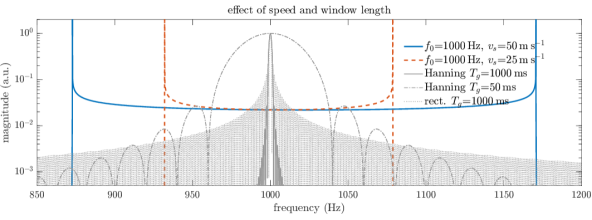
Figure 2: Overview over the integrand. Shown is the magnitude of $\hat{q}\!\left(\cdot\right)$ in Eq. (12) for ${f_{0}}=1000$ Hz and source speeds of $v_{s}=25$ m s^-1 (orange dashed) and $v_{s}=50$ m s^-1 (blue solid). The gray thin lines shows the Fourier transforms of a Hanning window: solid for $T_{g}=1000$ ms, dash-dotted for $T_{g}=50$ ms. The gray thin dotted line shows the Fourier transform of a rectangular window with $T_{g}=1000$ ms. The Fourier transforms of the windows are normalized to their peak amplitude for easier comparison.

2.4 Source localization

Up to now, all derivations used radial frequencies (${\omega_{m}^{\prime}}$, ${\omega_{0}}$) to avoid a cluttered notation due to factors of $2\pi$. From now on, for practical reasons the notation will be switched to regular frequencies (${f_{m}^{\prime}}$, ${f_{0}}$). With the transfer function $h_{n\ell}$ defined in Eq. (12), the total spectral complex amplitude at the receiver $n$ caused by all possible sources is given as:

$$\hat{p}_{n}[{f_{m}^{\prime}}] =\sum\limits_{\ell=1}^{L}a_{\ell}h_{n\ell}[{f_{m}^{\prime}}],$$ (13)

or if we collect the pressures at all microphones into one vector $\mathbf{\hat{p}}=(\hat{p}_{1},\dots,\hat{p}_{N})^{\top}$ and the unknown source strengths into $\mathbf{a}=(a_{1},\dots,a_{L})^{\top}$

$$\mathbf{\hat{p}}[{f_{m}^{\prime}}] =\mathbf{H}[{f_{m}^{\prime}}]\mathbf{a}.$$ (14)

As the difference between calculated values $\hat{\mathbf{p}}$ and measured sound pressures $\tilde{\mathbf{p}}$ should be as small as possible, the unknown amplitude vector ${\bf a}$ can be calculated by solving the least squares problem

$$\underset{\bf{a}\in\mathbb{C}}{\mathrm{min}}\lVert{\mathbf{H}}[{f_{m}^{\prime}}]{\bf a}-\tilde{{\mathbf{p}}}[{f_{m}^{\prime}}]\rVert_{2}^{2}.$$ (15)

This is the basic optimization problem for a single frequency ${\omega_{m}^{\prime}}$, which is typically strongly underdetermined as the number of microphones $N$ is much smaller than the number of potential sources $L$. In contrast to a stationary setting, where only one specific frequency bin ${f_{m}^{\prime}}\approx{f_{0}}$ can be used, the Doppler shift allows to use a spectral range $f^{\prime}_{m}\in[f_{-},f_{+}]:=[{f_{0}}(1+v_{s}/c)^{-1},{f_{0}}(1-v_{s}/c)^{-1}]$ in Eq. (15).

From this range it is possible to select $M$ discrete frequency bins, where $M$ is (up to some uncertainty at the frequency limits) restricted to $M\leq 1+(f_{+}\!-\!f_{-})\,\Delta\!f_{\mathrm{DFT}}^{-1}$. For a clearer notation these frequency bins are collected in a set $\Omega=\left\{{f_{m}^{\prime}}\,|\,f_{+}\!\leq\!{f_{m}^{\prime}}\!\leq\!f_{-}\right\}$ of cardinality $|\Omega|=M$. This approach has the advantage that instead of a highly underdetermined $N\times L$ system with $N\ll L$, a more stable $(N\cdot M)\times L$ system can be used for the least square approach. A suitable spectral range depends on many factors (cf. Fig. 1a and b) further restricting $f_{\mp}$. Setting the limits too wide may lead to some observations being more susceptible to corruption by background noise. How to determine a suitable set with regard to the size $M$ and choice of frequencies will be investigated in Sec. 3.

The case of the same single set $\Omega$ used for all microphones may be generalized to $N$ different sets $\Omega_{n}$ such that a different set of frequencies $f^{\prime}_{m(n)}$ is selected for each of the $N$ microphone measurements. In addition to increasing the number of observations by choosing $M>1$, regularization is an important topic when solving Eq. (15). In this work an standard Tikhonov regularization procedure combined with an L-curve approach is used to assess the effect of different parameters of the numerical model, e.g., source signal frequency, window length, speed, and choice of receiver frequencies. The resulting maps ${\bf a}$ show the spread of the point source, similar to a point-spread-function, and allow conclusions about how to control this spread (see Section 3).

After all measurement data have been transformed using a windowed DFT, $N\!\cdot\!M$ measurement points in the discrete frequency domain are selected comprising $N$ vectors $\tilde{\bf{p}}_{n}[\Omega_{n}]$ of dimension $M$ containing data according to the frequencies defined in the respective set $\Omega_{n}$. Applying the standard Tikhonov-regularization (also called ridge regression) minimizes the following expression:

$$\underset{\bf{a}\in\mathbb{C}}{\mathrm{min}}\sum\limits_{n=1}^{N}{\left\lVert\tilde{\bf{p}}_{n}[\Omega_{n}]-\sum\limits_{\ell=1}^{L}a_{\ell}h_{n\ell}[\Omega_{n}]\right\rVert_{2}^{2}}+\lambda\sum\limits_{\ell=1}^{L}\left|a_{\ell}\right|^{2}$$ (16)

or more compactly

$$\underset{\bf{a}\in\mathbb{C}}{\mathrm{min}}\lVert{\tilde{\mathbf{p}}_{\Omega}-{\mathbf{H}_{\Omega}}{\mathbf{a}}}\rVert_{2}^{2}+\lambda\lVert{\mathbf{a}}\rVert_{2}^{2},$$ (17)

where ${\mathbf{H}_{\Omega}}$ is of dimension $(M\cdot N)\times L$. Finding the optimal regularization parameter $\lambda$ is done using the L-curve approach [17] as implemented in the MATLAB library Regularization Tools [16].

2.5 Validation procedure

The following setup was created to validate the inverse approach. First, potential sources are assumed to be inside a 4 m$\times$4 m grid in the $x$-$z$-plane with an isotropic spacing of 0.05 m (i.e., an 80$\times$80 grid of source points) moving along the $x$-axis. The receiver positions were defined by a microphone array of 112 microphones with a geometry based on spirals and a diameter of approximately 1 m. The array was placed parallel to the moving source grid at distances of 4, 6, and 8 m in the $y$-direction. Fig. 3 shows the arrangement for the simulated data, where the source area is depicted at $t=0$ s. The algorithm’s performance is evaluated in a free 3D-space as well as above a fully reflecting half-plane located $z=-1$ m.

Figure 3: Area covered by the source grid (black rectangle) at time $t=0$ s and the area covered by the stationary microphone array (orange circle) which was used for the test cases.

The sound pressure at the microphones was created using simulated data of a uniformly moving mono-frequent point source with frequencies $f_{0}$ = 250, 500, 1000, and 2000 Hz, and source speeds of $v_{s}$ = 1, 10, 25, and 50 m s^-1. The source itself was located at the center of the source grid at $(x_{0},y_{0},z_{0})=(2,0,2)$ at time $t=0$ s. A simple time formulation was used to generate the test signal (cf., [8, 10]). For the experiments including a the reflecting half-plane (see Section 3.6) the source is mirrored at the plane $z=-1$ and added to the original source. All signals were generated using a sampling frequency of $f_{s}$=10 kHz, which is sufficiently high to accurately resolve the Doppler shifted frequencies for all $f_{0}$ and $v_{s}$ considered.

One important aspect of the numerical experiments is to evaluate different choices for $\Omega_{n}$ and the window function $g$ with respect to the performance as well as the gain in resolution by computing the convolution. For the time window $g$ Hanning windows of 7 different lengths $T_{g}$ ranging from 50 ms to 5000 ms were considered for the test signals as well as the transfer functions. The windows were centered around $t=0$ s. To calculate the integral in Eq. (12), the integration limits were set such that $\hat{g}(\omega_{m}^{\prime}-\omega)$ in Eq. (12) was more than 80 dB below the central peak $\hat{g}(0)$.

As the L-curve approach is known to occasionally lead to multiple corners and thus no clear optimal regularization value, a small amount of noise (SNR of 80 dB at the peak signal value) was added as suggested in [20]. There they showed, that poor L-curve shapes may occur due to “correlated noise” e.g. positioning errors. In the results presented here, the quadrature error in the frequency domain compared to the time domain approach used to generate the microphone data may be a reason for this effect. Overall, the small amount of noise lead to a much more stable regularization.

3 Results

3.1 Selection of observation frequencies $\Omega_{n}$

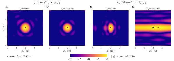
Figure 4: Source maps based on a single DFT bin $\Omega_{n}=\left\{f_{0}\right\}$ for each microphone. Shown are the amplitudes of the regularized solutions for a source with $f_{0}=1000$ Hz moving with two velocities: $v_{s}=1$ m s^-1 in panels a and b, $v_{s}=50$ m s^-1) in panels c and d. A short window ($T_{g}=50$ ms) was used in panels a and c, a long window with $T_{g}=1000$ ms was used in panels b and d. The black x denotes the true source position, the red circle the position of the detected maximum. The dynamic range is set to 20 dB and the maps are normalized to the respective peak amplitude.

It was already mentioned in the previous sections that for a mono-frequent source with frequency ${f_{0}}$ the measured signal at a stationary observer contains a frequency spectrum due to the Doppler effect. Important factors determining the width of this spectrum are the source frequency ${f_{0}}$, the speed of the source $v_{s}$, the length $T_{g}$ (c.f. Fig. 1) as well as the temporal position of the time window, and the distance between source and receiver. The choice of the sampling set(s) $\Omega_{n}$ of measurement frequencies used for the inversion of the transfer matrix is an important issue. In order to indicate the discrete nature of the DFT spectrum and the associated bandwidth $\Delta\!f_{\mathrm{DFT}}$ in the spectrum, the term DFT bin will be used for brevity when data at a specific frequency of the DFT spectrum is meant.

3.1.1 Single frequency bin

In a first setting, the single DFT bin closest to the source frequency was used for each microphone, i.e., $\Omega_{n}=\left\{f_{0}\right\},\forall n=1,\dots,N$ (up to a potential frequency mismatch due to the DFT bin spacing). This is closely related to the stationary case, where only the signal frequency is available. For the setting used in the evaluation the corresponding transfer matrix ${\mathbf{H}_{\Omega}}$ is of dimension 112$\times$6400 (number of receivers times number of potential sources). The entries of the matrix ${\mathbf{H}_{\Omega}}$ were calculated using Eq. (12). Considering an almost stationary source ($v_{s}=1$ m s^-1), the regularized inverse leads to the source maps ${\bf a}$ shown in Fig. 4a and b. Similar to conventional beamforming the detected source position is blurred, however, the peak (red circle) is located at true source position (black $\times$). The blurring of the source is roughly the same in $x$ and $z$.

The window length seems to have only a minor effect on the result although when going to even longer windows (5000 ms, not shown) the main lobe is more concentrated around the true source position but also two sidelobes with roughly -9 dB appear along the $x$-direction). Note that all source maps are normalized to the peak amplitude as in the current work only the spatial blurring was of interest.

For the fast moving situation (Fig. 4c and d), a number of effects occur. While the localization in the vertical direction ($z$) seems unaffected, a smearing occurs along the direction of motion for longer time windows (Fig. 4d, 1000 ms). For the given speed, the source moves 50 m during the period of 1000 ms while it only moves 2.5 m during 50 ms. Thus, the smearing along $x$ occurring for longer analysis window seems intuitively clear. On the other hand, the motion of the source as well as the spectral leakage caused by the DFT is, in theory, already considered in the transfer function. Apparently, the information contained at the same frequency across all microphones is not sufficient to lead to a reasonable estimate for the source map. In addition to the blurring, the peak (red circle) in the source strength map is also considerably displaced from the true source position (black x). As a consequence, restricting the inverse scheme to the same single DFT bin for all microphones does not yield satisfying results. Thus, in a next step a set of DFT bins arranged around the source frequencies is considered for the inversion process taking advantage of the spectral spread induced by the motion of the source. This has the effect of more observations and thus a less heavily underdetermined system of equations.

3.1.2 Regularly spaced bins

Before addressing the actual choice of frequencies, first, the available frequency range caused by the Doppler effect and the window needed to be determined. The equation for the Doppler shift of a moving source yields a maximum range given by $f_{0}(1\pm v_{s}/c)^{-1}$. For example, for $v_{s}=50$ m s^-1, ${f_{0}}=1000$ Hz, and a speed of sound $c=343$ m s^-1 this leads to a spectral range between approximately 873 Hz and 1170 Hz if a long enough temporal segment is considered. Shorter temporal segments lead to a reduced observed spread.

To allow for a better comparison of the source maps, the same frequency range was used for all analysis window lengths investigated (Hanning windows with $T_{g}=50$ ms to $T_{g}=5000$ ms). The range of frequencies for the upcoming analyses was restricted to $f_{-}=920$ Hz to $f_{+}=1120$ Hz. Close to these frequency bins a decay in amplitude of roughly 40 dB for $T_{g}=50$ ms (c.f. Fig. 1b) can be observed. For longer windows the decrease in amplitude at these frequencies is considerably smaller.

Based on the values for $f_{\pm}$, a suitable way to choose DFT bins from the available frequency range must be defined. The first scheme will employ the same set $\Omega_{n}$ of equally spaced DFT bins covering the predefined frequency range for each microphone. Fig. 5a and c show the results for selecting $M=5$ and Fig. 5b and d for $M=11$ (nearly) equally spaced frequency bins leading to matrix sizes of 560$\times$6400 and 1232$\times$6400, respectively. Note that a regular spacing is not always possible depending on the window length, frequency limits, and $f_{0}$. For $T_{g}=50$ ms, for example, the spacing of the DFT bins is given by $\Delta\!f_{\mathrm{DFT}}=20$ Hz and the restricted spectrum ranging from 920 Hz to 1120 Hz contains 11 bins as the limits also coincide with the bin frequencies. With this setting, a regular spacing is therefore only achieved for $M=2,3,6,$ or $11$. For longer windows, deviations from regular grids occur less often because $\Delta\!f_{\mathrm{DFT}}$ is smaller.

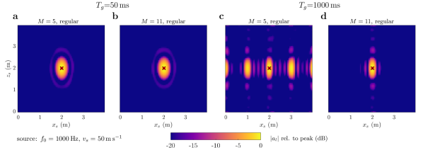
Figure 5: Source maps based on the same set of regularly spaced frequencies for each microphone. Shown are the amplitudes of the regularized solutions for ${f_{0}}=1000$ Hz and $v_{s}=50$ m s^-1 using a short window ($T_{g}=50$ ms) in panels a and b and a long window ($T_{g}=1000$ ms) in panels c and d. Panels a and c show the case of $M=5$, panels b and d the case of $M=11$ regularly spaced frequency bins. The black x denotes the true source position, the red circle the position of the detected maximum. The dynamic range is set to 20 dB and the maps are normalized to the respective peak amplitude.

A comparison of Figs 5a and b with Fig. 4c (all with a 50 ms Hanning window) shows much smaller sidelobes if more then one DFT bin is used. For the long Hanning window with length $T_{g}=1000$ ms (panels c and d in Fig. 5), the situation is more complex. Note that for $T_{g}=1000$ ms the DFT bin spacing is given by $\Delta\!f_{\mathrm{DFT}}=1$ Hz. For $M=11$ bins (panel d) the $x$-resolution is massively improved compared to the case where only one single bin was used (cf. Fig. 4d). If $M=5$, the main lobe is better localized around the true position but periodic sidelobes appear.

The periodicity of 1 m for the biggest lobes is a consequence of the frequency spacing chosen. Considering the range spanning 200 Hz, $M=5$ bins are equally spaced lying 50 Hz apart. This regular spacing of 50 Hz is equivalent to a period length of 20 ms which at $v_{s}=50$ m s^-1 is equivalent to a traveled distance of 1 m.

By the same rule, results from an inversion using 4 bins exhibit a periodicity of 0.75 m (not shown here). Interestingly, there also seems to be an observable damping acting on these “sidelobes". The seemingly shorter period of roughly 0.25 m results most likely from a periodic superposition of the sidelobes also occurring e.g., in Fig. 5d.

To investigate the periodicity and the slight damping in $x$ in more detail, a larger source grid ranging from 0 to 8 m with a smaller source grid spacing of 0.2 m (isotropic) was used. Clearly, in this setting there is a mismatch between the maximum and the true position. Furthermore, the decay is now better visible (Fig. 6), and comparing the 1000 ms (left, a) and the 5000 ms (right, b) window, the periodic sidelobes decay faster for the shorter window. The most likely explanation for this is the increased spectral leakage, and thus the increased contributions from neighboring frequencies.

For short windows the slight deviation of the used frequency grid from a regular spacing due to the coarser resolution may also be a reason for the faster decay of the sidelobes. This could explain the missing periodicity in Fig. 5a. For a window length of $T_{g}=50$ ms, the DFT bin spacing is $\Delta\!f_{\mathrm{DFT}}=20$ Hz. Therefore, no regular grid spacing could be with $M=5$ DFT bins, which in our setting would require a spacing of 50 Hz.

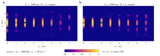
Figure 6: Effect of window length on the source map using the same set of $M=5$ regularly spaced frequencies for each microphone. Shown is the regularized solution for ${f_{0}}=1000$ Hz for using $T_{g}=1000$ ms window (a) and $T_{g}=5000$ ms (b). The black x denotes the true source position, the red circle the position of the detected maximum. The dynamic range is set to 20 dB and the maps are normalized to the respective peak amplitude.

3.1.3 Randomly selected bins

To avoid the periodicity problem, a different approach is suggested which uses a set of randomly selected frequency bins from the available frequency range. In detail, for each of the 112 microphones $M$ frequency bins are randomly chosen within the available frequency range. Thus, contrary to the approach using a regular spacing, DFT bins may vary across microphones. However, as already described in the case of regularly spaced bins, the number of available different frequency bins to choose from depends not only on the predefined frequency range but also on frequency resolution (which is the inverse of the chosen window length).

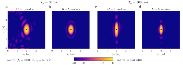
Figure 7: Source maps for different sets of random frequencies for each microphone. Shown are the amplitudes of the regularized solutions for ${f_{0}}=1000$ Hz and $v_{s}=50$ m s^-1 using a short window ($T_{g}=50$ ms) in panels a and b and a long window ($T_{g}=1000$ ms) in panels c and d. Panels a and c show the case of $M=1$ randomly assigned frequency bin per microphone, panels b and d the case of $M=5$ randomly assigned frequency bins per microphone. The black x denotes the true source position, the red circle the position of the detected maximum. The dynamic range is set to 20 dB and the maps are normalized to the respective peak amplitude.

Keeping the same values for $f_{\pm}$ as before, Fig. 7 illustrates the effect of using random frequencies. Clearly, the periodic effect has disappeared and, depending on $M$, the resolution in the $x$-direction can be largely improved, in particular for longer windows. For short time windows (panels a and b), there is no clear difference between using the same number of observations for a regular spacing (Fig. 5a) and a random selection (Fig. 7b) . This is most likely due to the relatively small number of available bins. For a range of 200 Hz and a window length of 50 ms this amounts to 11 bins and thus the random process will lead to a similar set of frequencies as the regular choice. In contrast, for $T_{g}=1000$ ms (panels c and d) 201 frequency bins are available per microphone and thus the set will be sufficiently random to omit periodic effects that occur for a regular spacing in this case. On the downside, for $M=1$ and the longer window, the vertical spreading increases compared to the previous cases using the signal frequency or regularly spaced bins. Setting $M=5$ leads to a similar vertical spread as for 11 equidistantly spaced DFT bins.

3.2 Effect of source frequency $f_{0}$

Already in the stationary case, the frequency ${f_{0}}$ of the source is an important factor affecting the localization performance of microphone arrays. The Doppler effect caused by a moving source additionally results in a spectral spreading of the observed frequency range that scales with ${f_{0}}$. Lower ${f_{0}}$ results in fewer available frequency bins that can actually be used for the inverse source localization, i.e., the choice of $M$ also depends on ${f_{0}}$.

In this section, the effect of the source frequency is investigated using values of ${f_{0}}$ = 250, 500, 1000, and 2000 Hz. As both, ${f_{0}}$ and $T_{g}$, affect $M$ the effect of ${f_{0}}$ cannot be investigated independently of $T_{g}$ and thus a range of values for $T_{g}$ from 50 ms to 5000 ms is considered. The same geometries and grids as in the previous section were used. A moving source with velocity $v_{s}=50$ m s^-1 was positioned at $(2,0,2)$ at $t=0$ s. Like in the previous section, the frequency range was set according to the speed using the same factor for all frequencies: $f_{-}=0.92{f_{0}}$ and $f_{+}=1.12{f_{0}}$. The localization performance for different $f_{0}$ was examined for varying window lengths and different values for $M$ ranging from 1 to 5. Note that in the case of $f_{0}=250$ Hz and $T_{g}=50$ ms only 3 DFT bins are available for the given frequency range. Thus, the maximum value for $M$ was limited to 3 for this case. The numerical experiments in the previous section were only based on one single set of random frequencies. In order to evaluate the variation of the results in dependence of the realization, 10 different random sets of $\Omega_{n}$ frequencies were generated for each case investigated. As in the previous section the analysis is based on the Tikhonov-regularized solution for the source grid.

To better illustrate the effect of the different parameters on the source localization, the -3 dB-contour around the true position (which deviated at most one grid point from the detected main peak for all cases) was determined for each resulting source map using the MATLAB-function contourc. The horizontal ($x$) and vertical ($z$) extension of the contour around the true position were determined and plotted in Fig. 8 as a function of the analysis time window length. In correspondence to beamforming, these two quantities will be referred to horizontal (denoted by solid lines) and vertical beamwidth (denoted by dashed lines). Each panel in Fig. 8 depicts the mean beamwidths across 10 random sets for frequencies ${f_{0}}$ = 250, 1000, and 2000 Hz, respectively. The shaded areas depict the maximum and minimum beamwidth across the 10 random sets. Colors and symbols distinguish different values for $M$. For conciseness, the results for ${f_{0}}=500$ Hz which lie between the results for 250 Hz and 1000 Hz are not shown here.

Figure 8: Beamwidth as a function of frequency, window length, and number of bins. Shown is the mean horizontal beamwidth (solid colored lines and symbols) and the mean vertical beamwidth (dashed colored lines and symbols) for the regularized solution and a threshold of 3 dB. Different values of ${f_{0}}$ are shown in panels a to c: 250, 1000, and 2000 Hz. The source speed was set to $v_{s}=50$ m s^-1. Colors and symbols denote different numbers of bins $M$.

As expected, the average resolution of the moving point source improves with increasing frequencies, i.e., the horizontal and vertical beamwidths decrease for increasing frequencies. There are, however, differences in the behavior of the horizontal and vertical beamwidth with respect to $T_{g}$ and $M$.

While the horizontal beamwidth is clearly reduced with increasing window duration, in particular for lower frequencies there is virtually no dependency on the number of frequency bins $M$.

The vertical beamwidth, on the other hand, is very large in comparison and no reduction or even an increase of the beamwidth is achieved when increasing the window length. Using an increasing number of frequency bins per microphone gradually improves the resolution in the vertical direction, at least for higher frequencies. For 250 Hz (Fig. 8a), the number of bins ($M$) has no relevant effect on the beamwidth which is probably a result of the reduced frequency range at low ${f_{0}}$ as there are simply not many different frequency bins to chose from. For 500 Hz (not shown) the reduction in horizontal beamwidth is also relatively small in the range of around 0.1 m and below.

Overall, Fig. 8 shows that the difference in beamwidth between $M=4$ and $M=5$ is relatively small, and there seems no point in going beyond $M=5$. A test calculation using $M=10$ did not yield any improvements compared to $M=5$. Concerning the variation of the estimates it is clearly shown that for $M=1$ the vertical beamwidth strongly varies with selected observation frequency bins $\Omega$ while for $M\!\!>1$ the localization performance seems almost independent of the actual set of frequencies. The reason for the very high variability and deviation for $M=1$ and 1000 Hz is, however, unclear.

3.3 Effect of source speed and distance between source and receiver

The second parameter affecting the Doppler effect is the source speed $v_{s}$. Lowering the speed from 50 m s^-1 to 25, 10, or even 1 m s^-1 leads to the results shown in Fig. 9. Setting the frequency ranges as in the case of 50 m s^-1, i.e., using $T_{g}=50$ ms as a reference and determining the closest bin to a decay of 40 dB from the spectral peak was not possible, as the limits were beyond the maximum Doppler shift. Thus the bin frequencies closest to this criterion but within the maximum Doppler shift were chosen. In each panel, the beamwidths are shown for a different velocity and different number of DFT bins $M$ as a function of the window length $T_{g}$. In all panels the source frequency was set to ${f_{0}}=1000$ Hz. For certain combinations with low source velocity (mainly $v_{s}=$1 m s^-1) and short windows, the frequency range caused by the Doppler shift is too small for the DFT sampling to choose sufficiently many DFT bins for $M>1$, hence no results can be shown for these cases.

The beamwidth in $x$ decreases with increasing window length up to a certain point but the number of used frequency bins does not affect the result very much. However, the number of DFT bins per microphone has some minor influence on the beamwidth in $z$. Using $M=5$ leads to estimates similar across all values for $v_{s}$ (Fig. 9 and Fig. 8b).

Interestingly, the effect of the window length on the horizontal beamwidth seems to depend on $v_{s}$, the decline of the curves seem to shift towards higher window lengths as the speed $v_{s}$ goes down and the final value is similar across different speeds. Although the exact relation was not determined, the data suggests that the shift is inversely proportional to the decrease in speed, i.e., halving the speed leads to the curve being “shifted” to double the window lengths. For example, the minimum window length for which the horizontal beamwidth does not decrease anymore is around 250 ms for $v_{s}=50$ m s^-1 (as shown in Fig. 8b), 500 ms for $v_{s}=25$ m s^-1 and around 1000 ms for $v_{s}=10$ m s^-1. For $v_{s}=1$ m s^-1 the point of leveling-off cannot be determined. This effect seems reasonable considering that signal portions containing high energy will become longer by essentially the same factor. Thus, a longer window will be better suited to cover the relevant signal portion. The variability of the beamwidth (shaded areas) is very low.

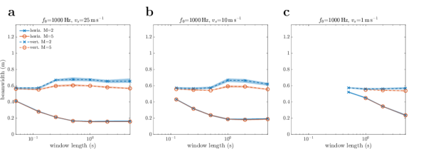
Figure 9: Beamwidth as a function of speed, window length, and number of bins. Shown is the mean horizontal beamwidth (solid colored lines and symbols) and the mean vertical beamwidth (dashed colored lines and symbols) for the regularized solution and a threshold of 3 dB. Different values of $v_{s}$ are shown in the panels a to c: 50, 25, and 1 m s^-1. The source frequency was set to ${f_{0}}=1000$ Hz. Colors and symbols denote the number of bins: blue x for $M=2$ and orange circles for $M=5$.

When the distance between the source plane and the receiver plane is increased to 6 m (Fig. 10a) or to 8 m (Fig. 10b), the vertical beamwidth increases, i.e., the source map becomes less localized (cf. Fig. 8b for 4 m distance) as is to be expected. In contrast, the much smaller horizontal beamwidth is essentially unaffected by the distance in $y$.

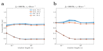
Figure 10: Beamwidth as a function of source-receiver distance in $y$, window length, and number of bins. Shown is the mean horizontal beamwidth (solid colored lines and symbols) and the mean vertical beamwidth (dashed colored lines and symbols) for the regularized solution and a threshold of 3 dB. Different values of the distance between sources and array are shown in the panels: 6 m (a) and 8 m (b). The source speed was set to $v_{s}=50$ m s^-1 and the source frequency to ${f_{0}}=1000$ Hz. Colors and symbols denote the number of bins: blue x for $M=2$ and orange circles for $M=5$.

3.4 Effect of the window function

As shown in Sec. 2, employing a DFT leads to a convolution of the 2.5D solution with the Fourier transform of the time window which needs to be evaluated. In general, this is a costly operation, as it requires the calculation of many 2D solutions. The length and type of the window $g$ affects the integration limits an thus has a huge influence on the computational effort of numerical convolution (cf. Fig. 2).

The necessity of including the window function is demonstrated in Fig. 11. Figs. 11c and d show the localization performance of the transfer function including the convolution with the window function, Figs.  11a and b without, i.e., the convolution with the window function is replaced by a simple point evaluation and thereby assuming an “ideal” Fourier transform $\hat{g}(\cdot)=\delta(\cdot)$. The DFT is still applied to the “measured” time signal. For short time windows (Figs. 11a vs. c) there is a clear improvement of localization performance, for longer time windows the difference in performance gets smaller because longer time windows are more concentrated around $\omega=0$ in the frequency domain.

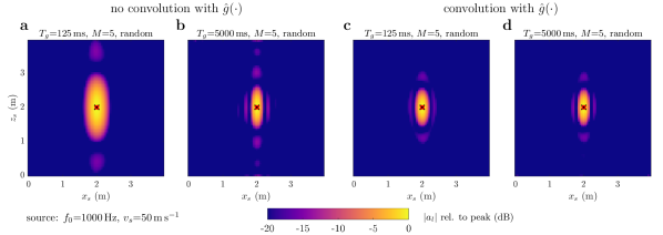
Figure 11: Effect of ignoring the spectral leakage on the source maps. Shown are the amplitudes of the regularized solutions for ${f_{0}}=1000$ Hz and $v_{s}=50$ m s^-1 using a short window ($T_{g}=125$ ms) in panels a and c and a long window ($T_{g}=5000$ ms) in panels b and d. All cases shown used $M=5$ randomly assigned frequency bins per microphone. Panels a and b show the results without taking the convolution into account in the transfer function, c and d show the case when the convolution is taken into account. The black x denotes the true source position, the red circle the position of the detected maximum. The dynamic range is set to 20 dB and the maps are normalized to the respective peak amplitude.

3.5 Effect of noise

Up to now, all examples were in a noise-free setting (up to the tiny amount of noise added for better convergence of the L-curve). To investigate the sensitivity of the presented approach to noise, bandpass-filtered Gaussian white noise was used. To test a slightly more realistic setting, the noise was not directly added to each measurement signal, as would be in the case of typical uncorrelated measurement noise related to the recording equipment. Rather, a stationary point source located at position $(20,10,1)^{\top}$ was assumed, which creates background noise that was added to the signal at each microphone. This way the noise at the different microphones is correlated mimicking the case of some noise source nearby. As the source to be detected is moving, the signal-to-noise-ratio is defined using the peak amplitude on the first channel of the array (close to the array center) compared to the energy of the stationary noise.

Only the case with $M=5$, $f_{0}=1000$ Hz, and $v_{s}=50$ m s^-1 was considered in this section. Note also that only a single realization of the noise was used.

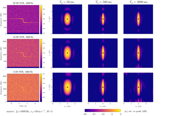
Figure 12: Effect of different SNRs on signal and source maps. The left column shows the time-frequency representations of noisy simulated pass-by signals at different noise levels (rows). From the second to the fourth column, the analysis window length is increased from 50 ms (second column) to 2000 ms (right column). The black x denotes the true source position, the red circle the position of the detected maximum. The dynamic range is set to 20 dB and the maps are normalized to the respective peak amplitude.

The first column in Fig. 12 shows the time-frequency representation of the “recorded” stimuli with different SNRs (different rows). Plots were generated using the functions dgt and plotdgt of the large time-frequency analysis toolbox (LTFAT, [30]). It can be seen that in particular the tails when the source is far away from the microphones are affected by the noise. In the remaining columns the effect of the noise on the source maps is shown for different levels of the SNR and different window lengths. The vertical blurring is more strongly affected by the SNR than the horizontal blurring. Fig. 13 shows this effect in more detail based on the 3-dB beamwidth as used before. Interestingly, the horizontal beamwidth is only affected by noise for shorter windows. For windows with length $T\geq 250$ ms different SNRs do not have an effect on the horizontal beamwidth. In contrast, the vertical beamwidth is mostly unaffected by the length of the window, however, the width gets smaller with increasing SNR. For $T_{g}=5000$ ms the increased noise level leads to a deterioration already at higher SNRs compared to shorter windows. For different random samples the general trends are essentially the same and thus only the results for a single random selection are shown to avoid cluttering in Fig. 13. For the vertical beamwidth, the variation is up to 10 cm but for SNRs of 20 dB and higher the variation lies below 5 cm. For the horizontal beamwidth the range of the varation is up to 2.5 cm but mostly below 1 cm.

The leveling-off of the vertical beamwidth for $T_{g}=5000$ ms at an SNR around 0 dB is to be treated with caution as the degree of the effect depends on the actual frequencies selected. A possible explanation is that at high noise levels spurious sidelobes start to appear (see for example the lower right subfigure in Fig. 12), which may influence the central lobe. The spurious sidelobes in turn are most likely caused by the increased noise contribution when using longer windows, as the tails of the signals disappear in the noise.

The reason for the opposite trend in the horizontal direction is not entirely clear. Most likely it is related to the general trend of the results that the horizontal beamwidth increases with lower $T_{g}$ (i.e. fewer bins) and thus these conditions may be more susceptible to noise.

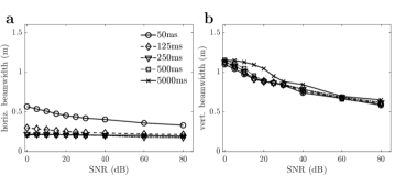
Figure 13: Effect of SNR on the beamwidth. The horizontal (a) and the vertical (b) beamwidth are shown as a function of the SNR and the analysis window length $T_{g}$ (symbols and line type).

3.6 Effect of a ground reflection

Using a numerical method like the 2.5D BEM has the advantage that it allows to include scattering objects into the source localization which may otherwise adversely affect the performance of standard beamforming approaches. Although the full BEM-framework is not used here, a straightforward example comprising a reflecting half-plane is shown to illustrate the general principle. The half-plane is located 1 m below the lower edge of the source grid. Thus, the assumed source lies 3 m above the plane resulting in considerable phase effects in the combination of source and mirrored source at the ground plane. The reference data for the moving point source is simply the sum of the moving point source and the mirror source. Similarly, the 2D Green’s function for the fully reflecting half-plane is a sum of 2 Hankel functions with different 2D-radii $r_{2}$.

Fig. 14 shows the results for a point source moving above a reflecting half-plane using the same parameters as in Fig. 7 with $M=5$. Figs. 14a and b show the results when the reflection is only considered in the reference signal at the microphones but not in the transfer matrix, in panels c and d the ground reflection is also considered when calculating the transfer matrix. If the reflection present in the “measured” signal is ignored when generating the transfer matrix, the result is much more blurred (Fig. 14a and b). The broader beamwidths in panels a and b are probably caused by the much higher regularization necessary to produce these maps. It is important to note that the L-curve did not work well in this mismatched condition. The corner detected without any limitation of the regularization lead to solutions which had little regularization and the resulting maps comprised mostly heavily scattered blobs or very strong interference patterns (not shown). Only with higher regularization maps appeared which were related to the true source distribution, however, at the cost of heavy blurring.

When considering the reflection in the transfer matrix (panels c and d), the beamwidth of the main lobe is much smaller, but sidelobes appear in the vertical direction. A closer inspection shows that the overall spread of the source map in panels c and d (including the main sidelobes) is only slightly larger compared to the pure free field case and that the sidelobes appear in a region similar to the source map identified in the free field case. Along the direction of motion $x$ only minor differences if any can be seen in the spread when comparing the case with (Fig. 14c and d) and without a reflecting half-plane (Fig. 7b and d).

Fig. 15 illustrates the differences between the half-plane and the free-field case in more detail. Shown are vertical sections in the center of the respective source maps ($x=2$ m) for the half-plane case for different window lengths (dashed, solid, and dash-dotted lines for $T_{g}=50,500,$ and $5000$ ms). For comparison, the source maps for the pure free field case (no mismatch) is shown for a window length of $T_{g}=5000$ ms (thin dotted line). The mismatched condition is not shown. When defining 3 dB for the cutoff of the central peak, the beamwidth in $z$ of the central peak is typically lower then in the free-field case. For higher frequencies (Fig. 15b and c) interference patterns appear along $z$. Comparing the width of the main lobe in the free-field and the combination of main lobe and first sidelobes in the half-plane case shows a similar range of the blurring in both cases.

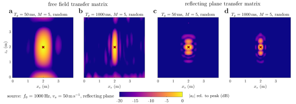
Figure 14: Source maps using a different set of $M=5$ random frequencies for each microphone for a moving source above a reflecting half-plane. Shown are the amplitudes of the regularized solutions for ${f_{0}}=1000$ Hz and $v_{s}=50$ $m\,s^{-1}$ using a short window ($T_{g}=50$ ms) in panels a and c and a long window ($T_{g}=1000$ ms) in panels b and d. Panels a and b show the inversion result when the reflecting plane is not considered in the transfer matrix (i.e. the free field case is used), panels c and d the case when it is considered. The dynamic range is set to 20 dB and the maps are normalized to the respective peak amplitude.

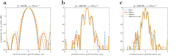
Figure 15: Comparison of amplitude profiles of central vertical sections of source maps for the half-plane and the free-field case. The source frequency varies from left to right: 250 Hz (a), 1000 Hz (b), and 2000 Hz (c). Colors and line types denote different window lengths. Thick lines show the half-plane case, the thin dotted line the free-field case. Data were normalized to a peak of 0 dB.

4 Discussion

In this work, an inverse source localization algorithm for mono-frequent uniformly moving sources was presented that acts entirely in the frequency domain and utilizes a 2.5D approach. Importantly, the effects caused by applying a discrete Fourier transform to the microphone recordings were taken into account when calculating the transfer functions from potential source points to the microphone positions. The main goal of this study was to investigate the effect of model parameters such as analysis window length, measurement frequency bins, speed and frequency of the source, and source-receiver distance on the localization performance. An off-the-shelf Tikhonov regularization was used for the inversion employing an L-curve approach to determine the optimal regularization parameter which was stabilized by adding a tiny amount of noise to the observations as suggested in the literature.

The performance of the algorithm was studied using simulated data of mono-frequent sources with different fundamental frequencies, speeds, and distances. These artificial data were generated using a time domain formulation which also allowed a direct assessment of the correctness of the frequency domain approach used for inversion. Overall, a good localization performance could be achieved with a placement error of at maximum 1 source grid point. The algorithm allows for the use of long windows, and thus a good spectral resolution even for high source speeds. Moreover, the algorithm even takes advantage of the motion allowing a better resolution along the direction of motion. A detailed analysis of the results lead to two key parameters affecting the performance: a) The inclusion of the effect of a windowed DFT into the transfer matrix via a convolution with the Fourier transform of the analysis window allows for a much better resolution of the point source, in particular for shorter windows. b) As the motion of the source leads to a spectral range at the receiver points the choice of observation frequency bins used in the comparison between measurement and numerical model has a profound effect on the algorithms performance.

It was shown that using only one single observation frequency equal to the source frequency for the inversion (as would be the case for stationary sources) leads to a large degree of blurring of the source map along the direction of motion, in particular for higher speeds and longer analysis windows. Using a regular frequency grid to cover the spectral range caused by the motion of the source lead to a better resolution along the direction of motion, but sometimes also induced periodicity in the results that depended on the source speed, the window length, and the chosen frequency spacing. This periodicity effect was overcome by using a different set of random observation frequencies for each microphone. The horizontal resolution, i.e., the resolution along the direction of motion, could be greatly improved compared to the source frequency setting without inducing periodicity in the solution. Also, longer analysis windows lead to less horizontal blurring, the effect being dependent on the source speed and frequency. However, the use of only one single random observation frequency per microphone lead to a comparatively poor vertical resolution and a high variability across different random choices. Increasing the number of observations by choosing more observation frequencies per microphone yielded a more reliable inversion of the transfer matrix and a decreased vertical blurring which then was similar across a range of source speeds including the almost stationary case.

The use of different noise levels illustrated that the horizontal blurring was largely unaffected by the signal-to-noise-ratio. In the vertical direction, however, the noise level strongly affected the vertical resolution.

Results for a reflecting ground showed the versatility of the principle approach and illustrated the importance of including surrounding structures that may affect the propagation. Importantly, the method can be expanded to more complex scenarios. A coupling with numerical methods like the BEM allows to include scattering objects as long as the assumption of a constant cross-section for the scatterer along the longitudinal dimension is fulfilled (e.g., a noise barrier).

The main drawback of the method is the high computational effort. In particular the numerical integration used for this proof-of-concept is far from optimal. Future work beyond the current state will focus on better quadrature approaches based, e.g., on methods for highly oscillatory integrands such as used in [22]. Also the choice of the measurement frequency range was not optimized for different window lengths and frequencies which will also be considered in the future. Currently, the approach is restricted to mono-frequent sources. Multiple such sources with different frequencies can be handled, as long as the frequency ranges are not overlapping. For overlapping signals, a joint inversion will be necessary which is ongoing work. Future work will also focus on more general broad-band signals. For this purpose, the computational effort required for a more general source signal becomes increasingly important. It is also planned to incorporate deconvolution methods or the direct use of methods enforcing some degree of sparsity. Current results show that the resolution can be controlled up to a certain degree, which will most likely also benefit sparse approaches.

References

- [1] M. Abramowitz and I. A. Stegun. Handbook of Mathematical Functions with Formulas, Graphs, and Mathematical Tables. Dover, New York, 9th edition, 1970.
- [2] D. Blacodon and G. Élias. Level estimation of extended acoustic sources using an array of microphones. 9th AIAA/CEAS Aeroacoustics Conference and Exhibit, 41(6), 2003.
- [3] T. F. Brooks and W. M. Humphreys. A deconvolution approach for the mapping of acoustic sources (DAMAS) determined from phased microphone arrays. J. Sound Vib., 294(4):856–879, 2006.
- [4] P. Chiariotti, M. Martarelli, and P. Castellini. Acoustic beamforming for noise source localization - Reviews, methodology and applications. Mech. Syst. Signal Pr., 120:422–448, 2019.
- [5] J. Christensen and J. Hald. Beamforming. Technical Report B&K Technical Review 1, B&K, 2004.
- [6] N. Chu, Q. Huang, L. Yu, Y. Ning, and D. Wu. Rotating acoustic source localization: A power propagation forward model and its high-resolution inverse methods. Measurement, 174:109006, 2021.
- [7] R. Cousson, Q. Leclère, M. A. Pallas, and M. Bérengier. A time domain CLEAN approach for the identification of acoustic moving sources. J. Sound Vib., 443(March):47–62, 2019.
- [8] A. T. de Hoop. Fields and waves excited by impulsive point sources in motion - The general 3D time-domain Doppler effect. Wave Motion, 43(2):116–122, 2005.
- [9] R. P. Dougherty. Extensions of DAMAS and benefits and limitations of deconvolution in beamforming. Collection of Technical Papers - 11th AIAA/CEAS Aeroacoustics Conference, 3:2036–2048, 2005.
- [10] D. Duhamel. Efficient calculation of the three-dimensional sound pressure field around a noise barrier. J. Sound Vib., 197(5):547–571, 1996.
- [11] D. Duhamel and P. Sergent. Sound propagation over noise barriers with absorbing ground. J. Sound Vib., 218(5):799–823, 1998.
- [12] J. Fakhraei, R. Arcos, T. Pàmies, and J. Romeu. 2.5D singular boundary method for exterior acoustic radiation and scattering problems. Eng. Anal. Bound. Elem., 143(June):293–304, 2022.
- [13] V. Fleury and J. Bulté. Extension of deconvolution algorithms for the mapping of moving acoustic sources. J. Acoust. Soc. Am., 129(3):1417–1428, 2011.
- [14] S. Gombots, J. Nowak, and M. Kaltenbacher. Sound source localization – state of the art and new inverse scheme. Elektrotechnik und Informationstechnik, 138(3):229–243, 2021.
- [15] S. Guerin and C. Weckmüller. Frequency-domain reconstruction of the point-spread function for moving sources. In Proceedings on CD of the 2nd Berlin Beamforming Conference (BeBeC), pages CD–ROM, 2008.
- [16] P. C. Hansen. Regularization Tools Version 4.0 for Matlab 7.3. Numerical Algorithms, pages 189–194, 2007.
- [17] P. C. Hansen and D. P. O’Leary. The Use of the L-Curve in the Regularization of Discrete Ill-Posed Problems. SIAM J. Sci. Comput., 14(6):1487–1503, 1993.
- [18] G. Herold and E. Sarradj. Performance analysis of microphone array methods. J. Sound Vib., 401:152–168, 2017.
- [19] M. Hornikx and J. Forssén. The 2.5-dimensional equivalent sources method for directly exposed and shielded urban canyons. J. Acoust. Soc. Am., 122(5):2532, 2007.
- [20] P. R. Johnston and R. M. Gulrajani. Selecting the corner in the L-curve approach to Tikhonov regularization. IEEE T. Bio.-Med. Eng., 47(9):1293–1296, 2000.
- [21] M. Kamrath, P. Jean, J. Maillard, J. Picaut, and C. Langrenne. Extending standard urban outdoor noise propagation models to complex geometries. J. Acoust. Soc. Am., 143(4):2066–2075, 2018.
- [22] C. Kasess, W. Kreuzer, and H. Waubke. An efficient quadrature for 2.5D boundary element calculations. J. Sound Vib., 382:213–226, 2016.
- [23] H. Li, D. Thompson, G. Squicciarini, X. Liu, M. Rissmann, F. D. Denia, and J. Giner-Navarro. Using a 2.5D boundary element model to predict the sound distribution on train external surfaces due to rolling noise. J. Sound Vib., 486:1–37, 2020.
- [24] F. Meng, Y. Li, B. Masiero, and M. Vorländer. Signal reconstruction of fast moving sound sources using compressive beamforming. Appl. Acoust., 150:236–245, 2019.
- [25] R. Merino-Martínez, P. Sijtsma, M. Snellen, T. Ahlefeldt, J. Antoni, C. J. Bahr, D. Blacodon, D. Ernst, A. Finez, S. Funke, T. F. Geyer, S. Haxter, G. Herold, X. Huang, W. M. Humphreys, Q. Leclère, A. Malgoezar, U. Michel, T. Padois, A. Pereira, C. Picard, E. Sarradj, H. Siller, D. G. Simons, and C. Spehr. A review of acoustic imaging methods using phased microphone arrays. CEAS Aeronaut. J., 10:197–230, 2019.
- [26] P. M. Morse and K. Uno Ingard. Theoretical acoustics. Princeton University Press, Princeton, NJ, 1987.
- [27] S. Oertwig, H. Siller, and S. Funke. SODIX for fully and partially coherent sound sources. In Proceedings on CD of the 9th Berlin Beamforming Conference (BeBeC), pages 1–15, 2022.
- [28] A. V. Oppenheim, R. W. Schafer, and J. R. Buck. Discrete-time signal processing. Pearson, Upper Saddle River, NJ, 2 edition, 1998.
- [29] J. Pizarro-Ruiz, E. P. García, and R. Gallego. Hypersingular boundary integral equation for harmonic acoustic problems in 2.5D domains with moving sources. Eur. J. Comput. Mech., 28(1-2):81–96, 2019.
- [30] Z. Průša, P. L. Søndergaard, N. Holighaus, C. Wiesmeyr, and P. Balazs. The Large Time-Frequency Analysis Toolbox 2.0. In Sound, Music, and Motion, LNCS, pages 419–442. Springer International Publishing, 2014.
- [31] A. Schuhmacher, J. Hald, K. B. Rasmussen, and P. C. Hansen. Sound source reconstruction using inverse boundary element calculations. J. Acoust. Soc. Am., 113(1):114–127, 2003.
- [32] T. Schumacher and H. Siller. Hybrid approach for deconvoluting tonal noise of moving sources. In Proceedings on CD of the 9th Berlin Beamforming Conference (BeBeC), pages CD–ROM, 2022.
- [33] P. Sijtsma. CLEAN Based on Spatial Source Coherence. Int. J. Aeroacoust., 6(4):357–374, 2007.
- [34] T. Suzuki. L1 generalized inverse beam-forming algorithm resolving coherent/incoherent, distributed and multipole sources. J. Sound Vib., 330(24):5835–5851, 2011.
- [35] The MathWorks Inc. MATLAB version: 9.14.0 (R2023a). Natick, Massachusetts, United States, 2023.
- [36] X. Wei and W. Luo. 2.5D singular boundary method for acoustic wave propagation. Appl. Math. Lett., 112:106760, 2021.
- [37] T. Yardibi, J. Li, P. Stoica, N. S. Zawodny, and L. N. Cattafesta. A covariance fitting approach for correlated acoustic source mapping. J. Acoust. Soc. Am., 127(5):2920–2931, 2010.
- [38] J. Zhang, G. Squicciarini, and D. J. Thompson. Implications of the directivity of railway noise sources for their quantification using conventional beamforming. J. Sound Vib., 459:114841, 2019.
- [39] J. Zhang, G. Squicciarini, D. J. Thompson, W. Sun, and X. Zhang. A hybrid time and frequency domain beamforming method for application to source localisation on high-speed trains. Mechanical Systems and Signal Processing, 200:110494, 2023.
- [40] C. Zhigang, S. Linbang, Y. Yang, and W. Guangjian. Non-negative least squares deconvolution method for mirror-ground beamforming. J. Vib. Control, 22(16):3470–3478, 2016.