Encoding Temporal Statistical-space Priors via Augmented Representation

Abstract.

Modeling time series data remains a pervasive issue as the temporal dimension is inherent to numerous domains. Despite significant strides in time series forecasting, high noise-to-signal ratio, non-normality, non-stationarity, and lack of data continue challenging practitioners. In response, we leverage a simple representation augmentation technique to overcome these challenges. Our augmented representation acts as a statistical-space prior encoded at each time step. In response, we name our method Statistical-space Augmented Representation (SSAR). The underlying high-dimensional data-generating process inspires our representation augmentation. We rigorously examine the empirical generalization performance on two data sets with two downstream temporal learning algorithms. Our approach significantly beats all five up-to-date baselines. Moreover, the highly modular nature of our approach can easily be applied to various settings. Lastly, fully-fledged theoretical perspectives are available throughout the writing for a clear and rigorous understanding.

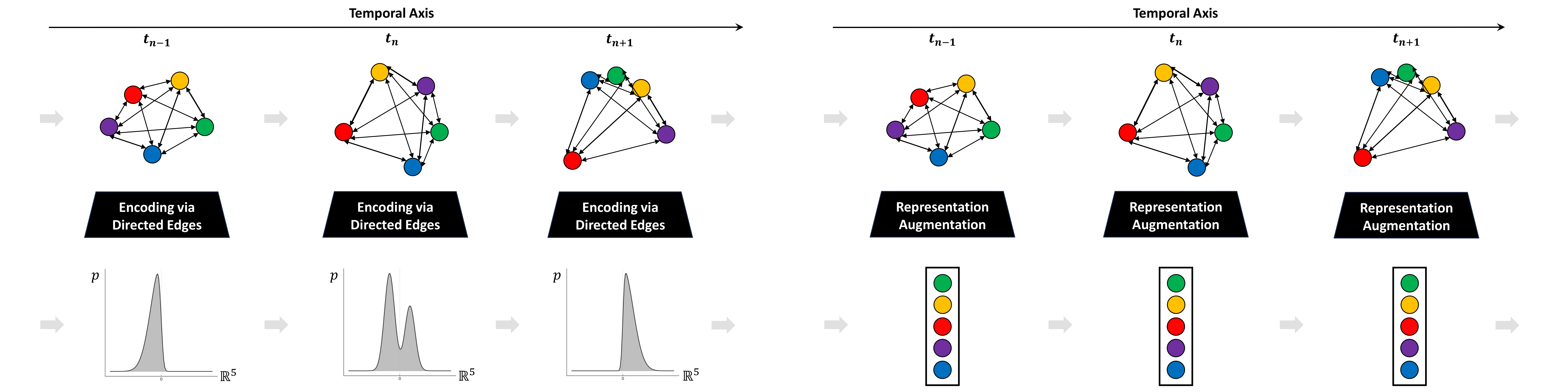
Figure 1. 5 variable example (left: theoretical view, right: representational view)

1. Introduction

Time series forecasting remains relevant in a voluminous range of domains, including finance and economics (Durairaj and Mohan, 2022), meteorology and climatology (Dimri et al., 2020), manufacturing and supply chain (Nguyen et al., 2021). Simple time series that are less stochastic and dependent on a tractable number of variables exist. However, the research community mainly focuses on time series with a high-dimensional dependence structure. Often, the true set of causal factors, $\mathcal{X}$, is intractable—i.e., unknown or known but impractical to compute. On top of this, complex time series structures, $p(\textbf{{y}}\in\mathcal{Y}|\textbf{{x}}\in\mathcal{X})$, often exhibit non-stationarity—making it even more challenging to model.

Nevertheless, initial multi-variate time series forecasting methods were model-based, like the vector autoregressive (VAR) model (Granger, 1969; Lütkepohl, 2005). The vector error correction model (VECM) extends the VAR model to handle cointegrated non-normal series (Johansen, 1991). Despite their widespread use, these statistical models have caveats, particularly vis-à-vis their underlying statistical property assumptions. Thus, any analysis using these models requires examination of these assumptions—especially the non-stationary assumption, potentially requiring transformations to the data.

In response, neural network-based sequential models have become popular in the past decade. Their main advantage is that a highly expressive universal function approximator flexibly captures high-dimensional non-linear statistical dependency structures (Liu et al., 2019). The most widely tested and verified for time series forecasting are Recurrent Neural Network (RNN) (Sherstinsky, 2020) architectures—with flagship examples being Long Short-Term Memory (LSTM) (Hochreiter and Schmidhuber, 1997) and Gated Recurrent Unit (GRU) (Cho et al., 2014). Both LSTM and GRU are part of our baseline.

More recently, with the out-performance of attention mechanism-based models like transformers in other sequential tasks such as natural language processing (NLP) (Galassi et al., 2020) and speech recognition (Alam et al., 2020), numerous transformer-based time series forecasting models have been developed. Some significant examples include the FEDformer (Zhou et al., 2022), Autoformer (Wu et al., 2021), Informer (Zhou et al., 2021), Pyraformer (Liu et al., 2021), and LogTrans (Li et al., 2019). Despite the research interest, a timely oral presentation at the AAAI conference, (Zeng et al., 2023) showed strong evidence that linear neural-network time series models, namely Linear, Normalization Linear (NLinear), and Decomposition Linear (DLinear), significantly outperform the aforementioned transformer-based models. This study showed robust multi-variate out-performance across Traffic, Electricity Transformer Temperature (ETT), Electricity, Weather, Exchange Rate, and Influenza-like Illness (ILI) datasets. All three (Zeng et al., 2023)’s models are included in our baseline.

Despite the success of neural-network-based approaches, we observed a lack of literature explicitly targeting the non-stationary and stochastic nature through a simple, theoretically elegant approach. In response, we develop a method that leverages neural networks while explicitly resolving the challenges in complex time series data.

Our contribution to the literature is summarized as follows:

• Develop an easily reproducible augmented representation technique, SSAR, that targets modeling complex non-stationary time series

• Clear discussion of the theoretical need for augmenting the input space and why it works well against baselines

• Theoretical discussion of the method’s inspiration—the data-generating process of high-dimensional time series structure

• To our knowledge, first to leverage (asymmetric) information-theoretic measures in modeling the statistical-space

• Out-sample improvement vis-à-vis performance and stability against up-to-date baselines: (i) LSTM, (ii) GRU, (iii) Linear, (iv) NLinear, (v) DLinear

• Out-sample empirical results tested on two data sets and two downstream temporal graph learning algorithms

• Appropriate ablation studies

• Present a theoretically unified view with related work, suggesting that SSAR implicitly smooths stochastic data

We emphasize reproducibility by uploading the data sets and source code on [insert GitHub link; will be included in the camera-ready version].

Notation. We let capital calligraphic letters denote sets (e.g., $\mathcal{X}$). Functions are often italicized where, e.g., $f:\mathcal{X}\mapsto\mathcal{Y}$ denotes function $f$ that maps from domain $\mathcal{X}$ to co-domain $\mathcal{Y}$. Capital blackboards are reserved for sets in number theory (e.g., $\mathbb{R}$). Vectors, matrices, and tensors are denoted in bold (e.g., a, A, A). Scalars are never bolded. Other notations follow machine learning community norms. If we diverge from these conventions, we explicitly state the notations in-text.

2. Related Works

Our work is related to temporal graph learning algorithms as our approach transforms a vector-based time series representation into a graph-based one. Then, a downstream graph learning algorithm is inducted to make predictions. In their most fundamental form of MLPs, neural networks are incompatible with input and output spaces represented as graphs. However, graphs naturally represent various real-world phenomena (Wu et al., 2022). E.g., social networks (Cao et al., 2020), chemical molecules (Wang et al., 2022), and traffic networks (Li and Zhu, 2021) are innately structured graphically. In turn, Graph Neural Networks (GNNs) bridge the gap between graphical structures and learning with neural networks. Unlike these works that have an existing set of edges $\mathcal{E}$, we derive $\mathcal{E}$ with historical values of vertices $\mathcal{V}$. The closest past work is (Xiang et al., 2022), where they generate Pearson correlation-based $\mathcal{E}$ with $\mathcal{V}$. However, their $\mathcal{E}$ is a proxy for inter-company relations specific to their domain and learning system. Additionally, their $e\in\mathcal{E}$ are non-directed and symmetric. On the contrary, our approach is (i) domain-agnostic, (ii) only uses our simple representation augmentation approach to statistically beat state-of-the-art, (iii) modular and compatible with an extensive list of downstream algorithms, (iv) also uses directed asymmetric measures for $\mathcal{E}$, and notably, (v) focused on the theoretical analysis of the representation augmenting mechanism.

3. Preliminary: Complex Time Series

There are three pervasive challenges of modeling complex time series for neural-network-based approaches—(i) incomplete modeling, (ii) non-stationarity, and (iii) limited access to the data-generating process.

Let $p(\textbf{{y}}^{t}\in\mathcal{Y}|\mathcal{X}^{t-M})$ be the true probability structure we want to learn. Here, vector $\textbf{{y}}^{t}$ is defined by the modeler as the variables of interest. Unlike $\textbf{{y}}^{t}$, $\mathcal{X}$ is intractable for complex problems as (i) it is too large to be computed realistically, but the more pressing problem is that (ii) it is unknown a priori. Therefore, we typically use heuristics or empirical evidence to identify $\hat{\mathcal{X}}$. Since we are forecasting, we use lagged values with $M$ indicating the temporal magnitude of the most lagged value. Then, with a learner parameterized by $\theta$, via maximum likelihood estimation we train for $\hat{p}_{\theta}(\textbf{{y}}^{t}\in\mathcal{Y}|\hat{\textbf{{x}}}^{t-m}\in\hat{\mathcal{X}}^{t-M})$ where $\hat{p}_{\theta}(\textbf{{y}}^{t}\in\mathcal{Y}|\hat{\textbf{{x}}}^{t-m}\in\hat{\mathcal{X}}^{t-M})\approx p(\textbf{{y}}^{t}\in\mathcal{Y}|\mathcal{X}^{t-M})$. In many cases, as $\mathcal{X}$ is intractable, we let $\hat{\textbf{{x}}}_{[,:]}:=\textbf{{y}}_{[,:]}$, making the input-space the lagged values of the output space. We also use this heuristic in our study and explain why this is a reasonable assumption in the appendix. Since $\hat{\textbf{{x}}}$ is a tractable approximation to the true input-space, we are faced with the partial observation and incomplete modeling problem. This fundamentally drives a significant portion of the stochasticity and poor performance in forecasting structures with a high-dimensional underlying structure. For domains that aggregate information on the global-level—like financial and climate time series, it is fair to assume that $|\mathcal{X}|\longrightarrow\infty$, dramatically raising the difficulty.

On top of this, we have a second, more pervasive challenge—non-stationarity. Non-stationarity is defined as $p(\textbf{{y}}^{t}|\textbf{{x}})\neq p(\textbf{{y}}^{t^{\prime}}|\textbf{{x}})$ where $t\neq t^{\prime}$. It could be argued that non-stationarity only exists due to the incomplete modeling mentioned above. Nevertheless, in real-world data, it is often the case that $p(\textbf{{y}}^{t}|\hat{\textbf{{x}}})\neq p(\textbf{{y}}^{t^{\prime}}|\hat{\textbf{{x}}})$ where $t\neq t^{\prime}$. This problem is summarized in Figure 1’s diagram on the left. Note that the distributions are 1-dimensional for a simplified visual view of the problem. In the example illustration in Figure 1, the distribution should be 5-dimensional. This poses a significant challenge to neural-network-based approximators $\hat{p}_{\theta}(\textbf{{y}}^{t}|\hat{\textbf{{x}}})$ as multi-layer perceptrons (MLPs), the fundamental building block of neural-network-based architectures inherently work on stationary data sets.

The last challenge for complex time series is closely tied to neural-network-based function approximators $F_{\theta}:\mathcal{X}\mapsto\mathcal{Y}$. The cost for a highly flexible function approximator $F_{\theta}$ is the large $|\theta|$. Consequently, as $|\theta|$ rises, the size of the data set $|\mathcal{D}|$ should also rise, allowing $F_{\theta}$ to generalize out-sample better. I.e., better approximate $p(\textbf{{y}}^{t}|\textbf{{x}})$. Ideally, $\frac{\partial|D|}{\partial|\theta|}>0$, but raising $|D|$ arbitrary is often intractable for complex time series. There are cases where reasonable simulators exist for the data-generating process $p(\textbf{{y}}^{t}|\textbf{{x}})$, especially when x is tractable and the probability transition function is well approximated by rules. A representative example is physics simulators in the robotics field (Makoviychuk et al., 2021), where the simulator models the real-world, $p_{sim}(\textbf{{y}}^{t}|\textbf{{x}})\approx p(\textbf{{y}}^{t}|\textbf{{x}})\Rightarrow$ the data is sampled to learn $\hat{p}_{\theta}(\textbf{{y}}^{t}|\hat{\textbf{{x}}})$. Correspondingly, we would require a world simulator for complex time series with an intractably high-dimensional data-generating process. Since we have no world simulator, raising $|\mathcal{D}|$ requires time to pass. Therefore, we are often restricted with a finite, lacking $\mathcal{D}$.

1:Input: $\textbf{{D}}_{raw}$, $m(\cdot)$, $w_{s}$

2:Output: $\mathbfcal{G}:=\{\mathcal{G}_{0},...,\mathcal{G}_{T-w_{s}-1}\}$

3:Function SSAR($\textbf{{D}}_{raw}$, $m(\cdot)$, $w_{s}$):

4:

5:$\textbf{{D}}_{processed}\longleftarrow DataProcess(\textbf{{D}}_{raw})$

6:$\mathcal{F}\longleftarrow\textbf{{D}}_{processed}.get\_feature\_set()$

7:$T\longleftarrow\textbf{{D}}_{processed}.get\_total\_timesteps()$

8:$\mathbfcal{G}\longleftarrow\{\}$

9:

10:for $t\in T\backslash\{0,...,w_{s}-1\}$ do

11:     $\mathcal{G}_{t}\longleftarrow di\text{-}Graph()$

12:     for $\forall permutation\langle f_{i},f_{j}\rangle\in\mathcal{F}$ do

13:         if $f_{i}\notin\mathcal{G}_{t}.nodes$ then

14:              $\mathcal{G}_{t}.add\_node(f_{i})$

15:         end if

16:         if $f_{j}\notin\mathcal{G}_{t}.nodes$ then

17:              $\mathcal{G}_{t}.add\_node(f_{j})$

18:         end if

19:         $weight\longleftarrow|m(\langle f_{i},f_{j}\rangle,w_{s},t)|$ 

20:         if weight $\neq$ 0 then

21:              $\mathcal{G}_{t}.add\_edge(f_{i}\rightarrow f_{j},weight)$ 

22:         end if

23:     end for

24:     $\mathbfcal{G}.append(G_{t})$

25:end for

26:

27:return $\mathbfcal{G}$

28:End Function

Algorithm 1 SSAR

4. Methodology

4.1. Statistical-space Augmented Representation

In response to the three challenges stated in the preliminary, we apply our method, SSAR. We rigorously examine how SSAR overcomes each challenge in section 4.3. A high-level overview of SSAR is as follows: (i) select a statistical measure, (ii) compute the statistical measure $m(\textbf{{y}}|\textbf{{x}},t,w_{s})\ \forall t$ with sliding window $w_{s}$, (iii) generate a graph $\mathcal{G}^{t}$ where vertices $n\in\mathcal{V}^{t}$ represent variables at $t$, and weight of edges $w(e)$, where edges $e\in\mathcal{E}^{t}$, represent $m(\textbf{{y}}|\textbf{{x}},t,w_{s})$. Then, with spatiotemporal graph $\mathbfcal{G}:=\bigcup_{t}\mathcal{G}^{t}$, we can apply any temporal graph learning algorithm that makes temporal node prediction to solve the forecasting problem. We examine SSAR more rigorously below.

As seen in Figure 1, right, $\textbf{{SSAR}}:\mathcal{D}\mapsto\mathbfcal{G}$ where the original time series data $\mathcal{D}$ is in vector form $\textbf{{d}}\in\mathcal{D}$. The per time step functional view would be $\mathcal{G}^{t}\leftarrow\textbf{{SSAR}}(\textbf{{d}}^{[t-w_{s}:t]}\in\mathcal{D})$. The pseudo-code of $\textbf{{SSAR}}(\cdot)$ is available in Algorithm 1. $\forall t\ \textbf{{d}}^{t}$ is transformed into a weighted, directed graph $\mathcal{G}^{t}=\langle\mathcal{V},\mathcal{E},\mathcal{W}\rangle$ where $\mathcal{V}$ is the set of nodes, $|\mathcal{V}|=N$, $\mathcal{E}$ is the set of directed edges, $|\mathcal{E}|=N^{2}-N$, and the weighted adjacency matrix $\mathcal{W}\in\mathbb{R}^{N\times N}$. Here, each node $n\in\mathcal{V}$ represents a variable (scalar) $\in\hat{\textbf{{x}}}=\textbf{{y}}$. Each $e\in\mathcal{E}$ is a 2-tuple denoted $\langle n_{i},n_{j}\rangle$, $i\neq j$, with each tuple corresponding to a permutation pair of nodes. The cardinality of $\mathcal{E}$ is $N^{2}-N$, as each permutation pair has one directed edge. In other words, a non-ordered pair would correspond to two directed edges, $e_{ij}:n_{i}\rightarrow n_{j}$, and $e_{ji}:n_{j}\rightarrow n_{i}$. $|\mathcal{E}|$ can be $\lessgtr N^{2}-N$, with $|\mathcal{E}|>N^{2}-N$ being the case where $\exists$ numerous directed edges for a given ordered pair, and $|\mathcal{E}|<N^{2}-N$ being the case where not all ordered pairs are linked via a directed edge. Our $\mathcal{G}^{t}$’s $|\mathcal{E}|=N^{2}-N$ as each permutation pair corresponds to a single directed edge, and nodes cannot direct to themselves. I.e., $\mathcal{G}^{t}$ is irreflexive. Given that the size of $\mathcal{W}$ is computed excluding the diagonal elements, where $w\in\mathcal{W}$, $w\geq 0\in\mathbb{R}$, $\mathcal{W}$ is equivalent in size to $\mathcal{E}$ as each $e_{ij}$ maps to a single $w_{ij}$. I.e., $W:\mathcal{E}\mapsto\mathcal{W}$. Here, $w^{t}(n_{j}\rightarrow n_{i})\leftarrow m(n_{i}|n_{j},t,w_{s})$. An intuitive visualization is available in Figure 2.

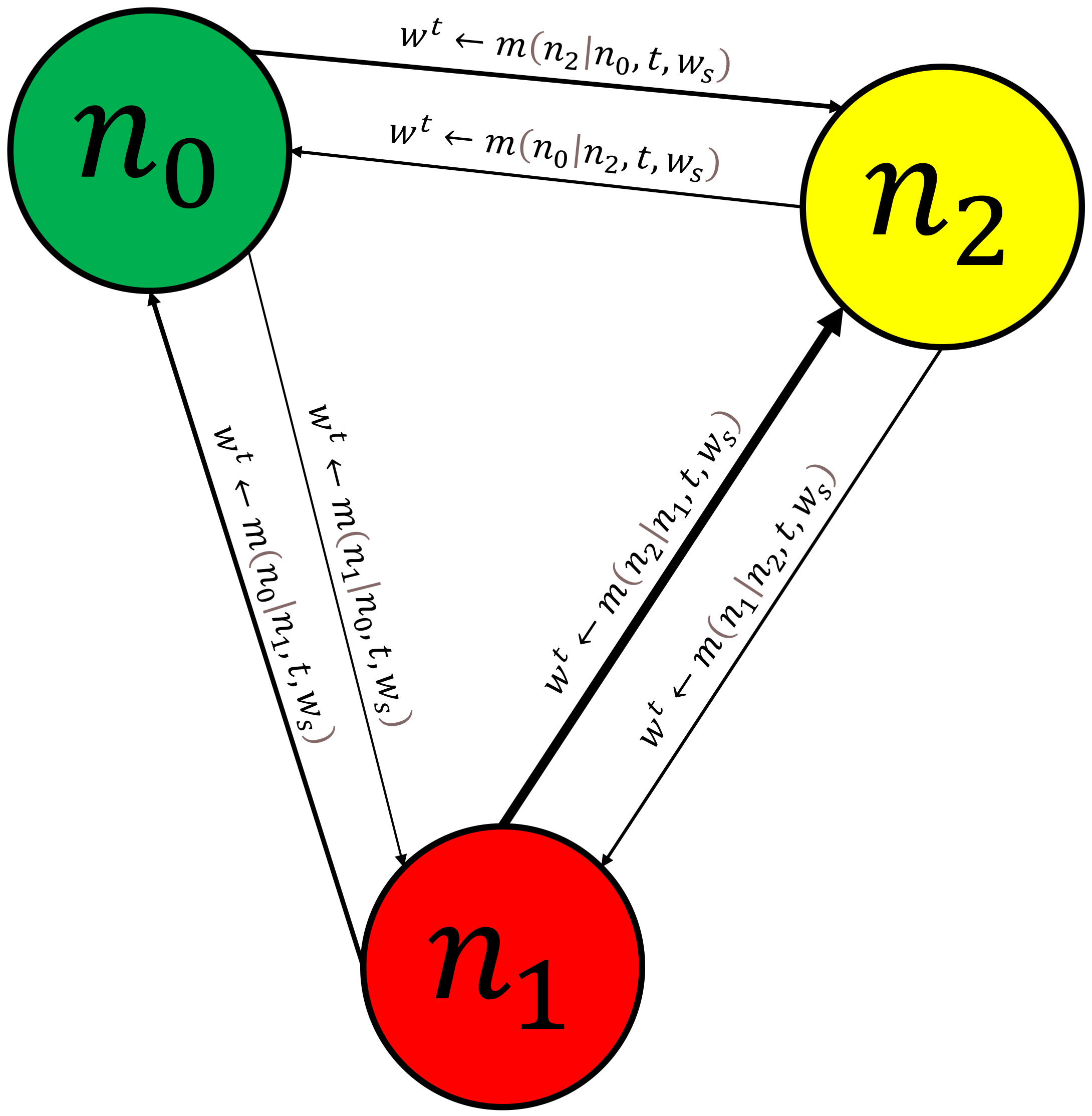
Figure 2. Sample $\mathcal{G}^{t}$, $N:=3$

4.2. Data-generating Process

SSAR is fundamentally inspired by the data-generating process of complex time series. The data-generating process in traditional machine learning literature refers to a theoretical $p(\cdot)$. If we have access to $p(\cdot)$, we can sample data $D\sim p(\cdot)\Rightarrow$ approximate $\hat{p}_{\theta}(\cdot)$ via maximum likelihood estimation of $D$. On a different note, this abstracted discussion aims to shed light on how a true $p(\cdot)$ is derived in the real world. I.e., it aims to hypothesize on the mechanisms underlying $p(\cdot)$, then describe how it inspires our approach. Note that this section (4.2.) is highly theoretical and can be safely skipped if the reader is purely interested in the application of SSAR.

First, we assume that we are dealing with complex time series described in the preliminary.

Definition 4.1.

Define complex time series which is causal in nature as $p(\textbf{{y}}^{t}\in\mathcal{Y}|\mathcal{X}^{t-M})$ where $\mathcal{X}$ is intractable—i.e., $|\mathcal{X}|\longrightarrow\infty$.

Much like how the existence of $p(\cdot)$ is theoretical, the notion of $\mathcal{X}$ is theoretical, as the (non-mathematical) notion of variables in $\mathcal{X}$ are man-made. Meaning virtually any arbitrary degree of granularity can be applied to describe $\mathcal{X}$. I.e., $|\mathcal{X}|$ can be arbitrarily raised larger until we reach the smallest units of the physical world. For example, We could say that a high-level event, such as a time COVID-19 was raised as a national threat, is a $x\in\mathcal{X}$, or we could break this down into more granular-level events, such as patient zero contracting the virus, or even further granular into physical-level events.

Nevertheless, given a true $p(\textbf{{y}}^{t}|\mathcal{X}^{t-M})$, we let $\mathcal{X}_{meas}\subset\mathcal{X}$ and $\mathcal{X}_{meas^{\prime}}\subset\mathcal{X}$ being the subset of $\mathcal{X}$ that humans digitally measured in time series format, and the remainder, respectively. $\mathcal{X}_{meas}\cup\mathcal{X}_{meas^{\prime}}\equiv\mathcal{X}$ and $\mathcal{X}_{meas}\cap\mathcal{X}_{meas^{\prime}}=\emptyset$. In the case of learning algorithms that require a numerical input and output space, naturally, $\textbf{{y}}^{t}\in\mathcal{Y}\subseteq\mathcal{X}_{meas}$ and $\hat{\textbf{{x}}}\in\mathcal{X}_{meas}$. We define any mechanism within $\mathcal{X}_{meas}$ as endogenous to the system and any mechanism within $\mathcal{X}_{meas^{\prime}}$ as exogenous to the system. Since humanity does not digitally track every single real-world physical change, each endogenous change can be traced back to some exogenous change. With this backdrop, we can imagine all numerical variables available to us digitally as a system that absorbs an arbitrary amount of exogenous shocks $\forall t$.

Let (non-mathematical) variable $x_{meas^{\prime}}\in\mathcal{X}_{meas^{\prime}}$, and (mathematical) variable $x_{meas}\in\mathcal{X}_{meas}$. Then, a simplified view of the data-generating process can be visualized in Figure 3. Each node at the top of the diagram represents $x_{meas^{\prime}}\in\mathcal{X}_{meas^{\prime}}$ while each node at the bottom represents $x_{meas}\in\mathcal{X}_{meas}$. Within the diagram, $|\mathcal{X}_{meas^{\prime}}|\longrightarrow\infty$ is indicated via ”…”. Blue and purple edges show causal chains in the real physical world. Each dotted edge represents an exogenous shock to the endogenous system. Non-dotted green and red edges at each time step represent $p(\textbf{{y}}_{meas}^{t}|\textbf{{x}}_{meas}^{t-1})$. However, since $\exists p(\textbf{{x}}_{meas}^{t}|\textbf{{x}}_{meas^{\prime}}^{t-1})$ which is unknown as the conditional variable is unknown,

$$p(\textbf{{y}}_{meas}^{t}|\textbf{{x}}_{meas}^{t-1})\Rightarrow p(\textbf{{y}}_{meas}^{t}|p(\textbf{{x}}_{meas}^{t-1}|\textbf{{x}}_{meas^{\prime}}^{t-2})).$$

Under this view, all complex time series are inherently non-stationary and, consequently, incompatible with models assuming stationarity. Consequently, for models that require stationary data, we require some tractable function $f(\cdot),\ s.t.,$

$$f(\cdot)\approx p(\textbf{{x}}_{meas}^{t-1}|\textbf{{x}}_{meas^{\prime}}^{t-2}).$$

In the following section, we take inspiration from the inherently di-graphical nature of the data-generating process, as exemplified in Figure 3, to theoretically unpack our method.

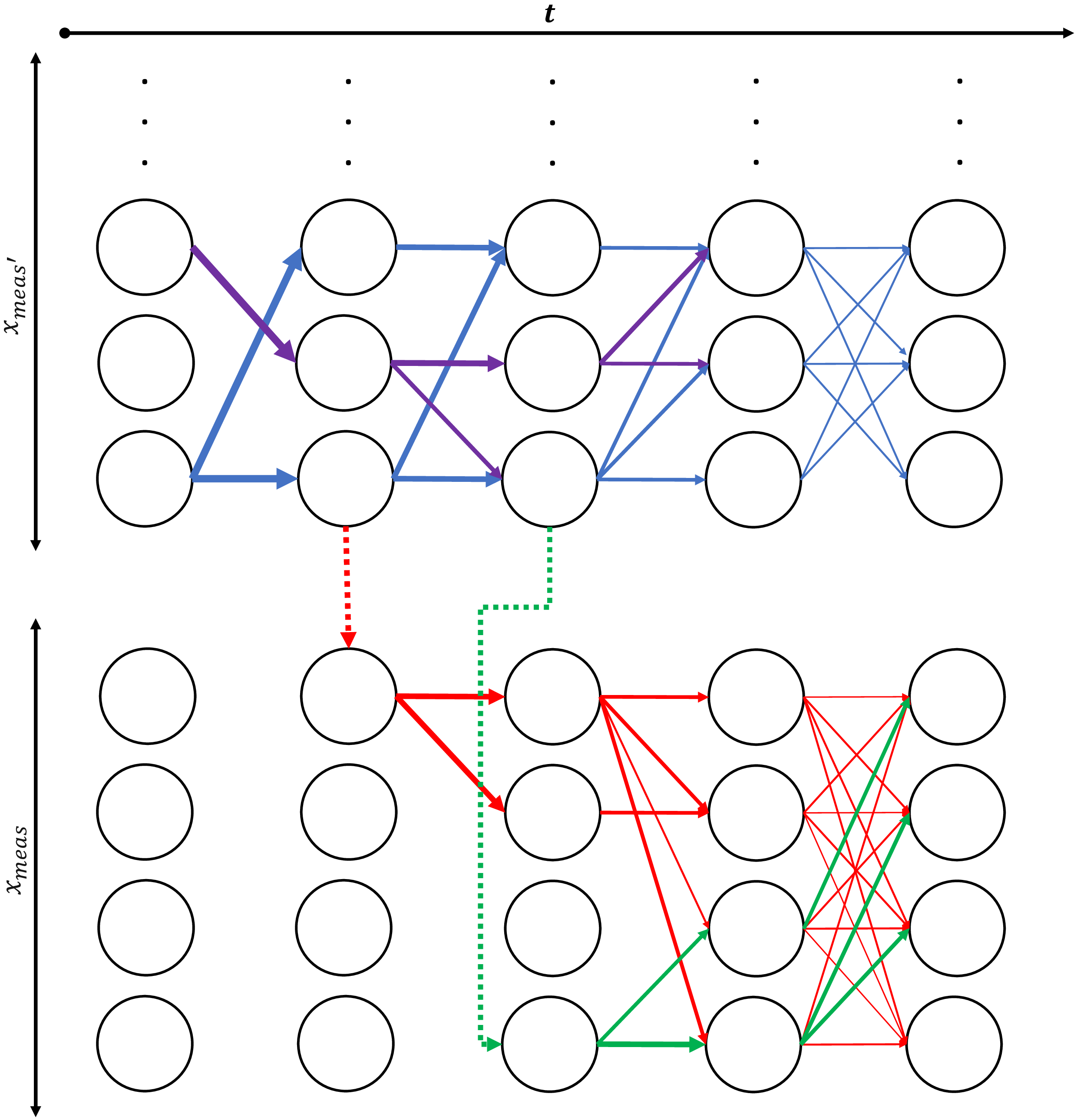
Figure 3. Real-world causal chains

4.3. Prior Encoding: Theoretical View

By the universal approximation theorem of neural networks (Cybenko, 1989; Hornik et al., 1989), any stationary mapping can be approximated by neural networks. Then, what are the limitations of existing neural-network-based approaches, and how does our approach remedy these shortcomings? MLPs and all subsequent architectural innovations based on MLPs already implicitly model the high-dimensional statistical-space.

$$\textbf{O}_{0}:=\alpha(\textbf{W}_{0}^{T}\textbf{X}+\textbf{{b}}_{0}),$$

$$\textbf{O}_{1}:=\alpha(\textbf{W}_{1}^{T}\textbf{O}_{0}+\textbf{{b}}_{1}),$$

$$\textbf{O}_{2}:=\sigma(\textbf{W}_{2}^{T}\textbf{O}_{1}+\textbf{{b}}_{2}),$$

where $\theta=\{\textbf{W},\textbf{b}\}$, X is the input tensor, and $\alpha,\sigma$ are non-linear activations. It is evident that as neural networks are directed graphs, the explicit representation provided by SSAR, as visualized in Figures 1 and 2, can be implicitly represented by (3). Despite the implicit representation, we choose to encode an explicit representation as a Bayesian prior $p(\theta)$. Under the Bayesian view of learning from data,

$$p(\theta|\mathcal{D}):=\frac{p(\mathcal{D}|\theta)p(\theta)}{p(D)}.$$

This inductive bias—if correct, can be helpful for generalized performance when $|\mathcal{D}|\ll\infty$. We have described in the preliminary why complex time series often have finite $\mathcal{D}$, and it is challenging, if not impossible, to raise the size of $\mathcal{D}$.

Our prior encoding $\forall t$, as visualized in Figure 1, left, aids learning via overcoming non-stationarity. The stationarity problem is described by $p(\textbf{{y}}^{t}|\hat{\textbf{{x}}})\neq p(\textbf{{y}}^{t^{\prime}}|\hat{\textbf{{x}}})$ where $t\neq t^{\prime}$. Since we are learning the distribution $\hat{p}_{\theta}(\textbf{{y}}^{t}|\hat{\textbf{{x}}})$, to capture the non-stationarity, a natural approach would be to add a second parameter, a regime vector r, resulting in learning $\hat{p}_{\theta}(\textbf{{y}}^{t}|\hat{\textbf{{x}}},\textbf{{r}}\leftarrow r(\textbf{{y}}^{t}|\hat{\textbf{{x}}}))$. A common approach is learning $r_{\theta_{r}}(\cdot)$. In this case,

$$\hat{p}_{\theta}(\textbf{{y}}^{t}|\hat{\textbf{{x}}},\textbf{{r}}\leftarrow r_{\theta_{r}}(\textbf{{y}}^{t}|\hat{\textbf{{x}}})),$$

$$\therefore\theta^{tot}:=\theta\cup\theta_{r},\ \Rightarrow|\theta^{tot}|>|\theta|\because|\theta_{r}|>0.$$

As mentioned above, since we have a small $\mathcal{D}$ relative to the $|\mathcal{X}|\longrightarrow\infty$, it is undesirable to raise the degrees of freedom without further sampling $\mathcal{D}\sim p(\cdot)$. Since we cannot further sample at a given point in time without the passage of time, we are left to explore alternative solutions.

An ideal alternative is letting a statistical-space relationship at $t$ proxy for $r(\cdot)$—i.e., $m(\textbf{{y}}^{t}|\hat{\textbf{{x}}},t,w_{s})\approx r(\textbf{{y}}^{t}|\hat{\textbf{{x}}})$. But, like $r(\textbf{{y}}^{t}|\hat{\textbf{{x}}})$, $m(\textbf{{y}}^{t}|\hat{\textbf{{x}}},t,w_{s})$ is unknown a priori. In this case, like $r_{\theta_{r}}(\cdot)$, we would require a learned approximation $m_{\theta_{m}}(\cdot)$, raising the size of aggregate parameters.

A reasonable and tractable approximation known a priori that does not raise the parameter count is,

$$m(\textbf{{y}}^{t-1}|\hat{\textbf{{x}}},t-1,w_{s})\approx m(\textbf{{y}}^{t}|\hat{\textbf{{x}}},t,w_{s})\approx r(\textbf{{y}}^{t}|\hat{\textbf{{x}}}).$$

Given that the time steps $t$ are sufficiently granular, it can be assumed that $m(\textbf{{y}}^{t-1}|\hat{\textbf{{x}}},t-1,w_{s})$ closely approximates $m(\textbf{{y}}^{t}|\hat{\textbf{{x}}},t,w_{s})$. We hypothesize that the trade-off between parameter count and approximation via $t-1$ is advantageous to the learning system.

Even after identifying a reasonable regime-changing approximator, a secondary problem persists. Representing and passing $m(\textbf{{y}}^{t-1}|\hat{\textbf{{x}}},t-1,w_{s})$ via Euclidean geometry, i.e., grid-like representation, significantly reduces the spatial information inherent to $m(\textbf{{y}}^{t-1}|\hat{\textbf{{x}}},t-1,w_{s})$. A natural representation is graphical, like Figure 3—therefore, we approximate (8) with (9) via (10), (11), and (12). This transformation via augmenting the representation theoretically summarizes SSAR.

$$\hat{p}_{\theta}(\textbf{{y}}^{t}|\hat{\textbf{{x}}},\textbf{{r}}\leftarrow r(\textbf{{y}}^{t}|\hat{\textbf{{x}}})),$$

$$\hat{p}_{\theta}(\textbf{{v}}^{t}\in\mathcal{V}|\textbf{{v}}^{t-M}\in\mathcal{V},\textbf{{e}}^{t-M}\in\mathcal{E}),$$

$$\textbf{{v}}^{t}:=\textbf{{y}}^{t},$$

$$\textbf{{v}}^{t-M}:=\hat{\textbf{{x}}},$$

$$\textbf{{e}}^{t-M}\approx\hat{\textbf{{r}}}\approx\textbf{{r}},$$

$$\text{where}\ \mathcal{E}\leftarrow m(\textbf{{y}}^{t-1}|\hat{\textbf{{x}}},t-1,w_{s}).$$

4.4. Statistical-space Measures

We compute $m(\textbf{{y}}^{t-1}|\hat{\textbf{{x}}},t-1,w_{s})$ in six ways. The set of measures and corresponding abbreviation $\mathcal{M}:=$ {Pearson correlation: Pearson, Spearman rank correlation: Spearman, Kendall rank correlation: Kendall, Granger causality: GC, Mutual information: MI, Transfer entropy: TE}. This set can be further divided into correlation-based $\mathcal{M}^{sym}$ and causal-based $\mathcal{M}^{asym}$ measures, which are symmetric and asymmetric, respectively. $\mathcal{M}^{sym}:=$ {Pearson, Spearman, Kendall} $\subset\mathcal{M}$, $\mathcal{M}^{asym}:=$ {GC, MI, TE} $\subset\mathcal{M}$, $\mathcal{M}^{sym}\cup\mathcal{M}^{asym}\equiv\mathcal{M}$, $\mathcal{M}^{sym}\cap\mathcal{M}^{asym}=\emptyset$. Symmetric measure refers to $m(n_{j}|n_{i})=m(n_{i}|n_{j})\ \forall\langle i,j\rangle\in\mathcal{E},i\neq j$. Asymmetric refers to the case where $m(n_{j}|n_{i})\neq m(n_{i}|n_{j})$. The asymmetric case is, in theory, most appropriate for our use case, as it uses only lagged values, making them a proxy for causal effects. It is also more natural to embed $m^{asym}(\cdot)\in\mathcal{M}^{asym}$ as weights as $m^{asym}:\mathcal{X}\times\mathcal{Y}\mapsto\mathbb{R}_{\geq 0}$. On the other hand, $m^{sym}:\mathcal{X}\times\mathcal{Y}\mapsto[-1,1]$, therefore, we let $m^{sym}\leftarrow|m^{sym}|$. We empirically test all six.

The hyperparameter $w_{s}$ is inherent to SSAR, as it is required to compute $m(\cdot)$. An additional hyperparameter $\exists\forall$ sequential neural-network-based downstream algorithms—$M$. scalar $M$ represents the number of previous time steps fed into the model. In our case, $M$ represents the number of historic graphs as $\exists\mathcal{G}^{t}\ \forall t$. When combining SSAR with a downstream temporal graph learning algorithm, there are two sliding windows—$w_{s}$ and $M$. An intuitive visualization is provided in Figure 4. The computational details $\forall m(\cdot)\in\mathcal{M}$ are available in the Appendix.

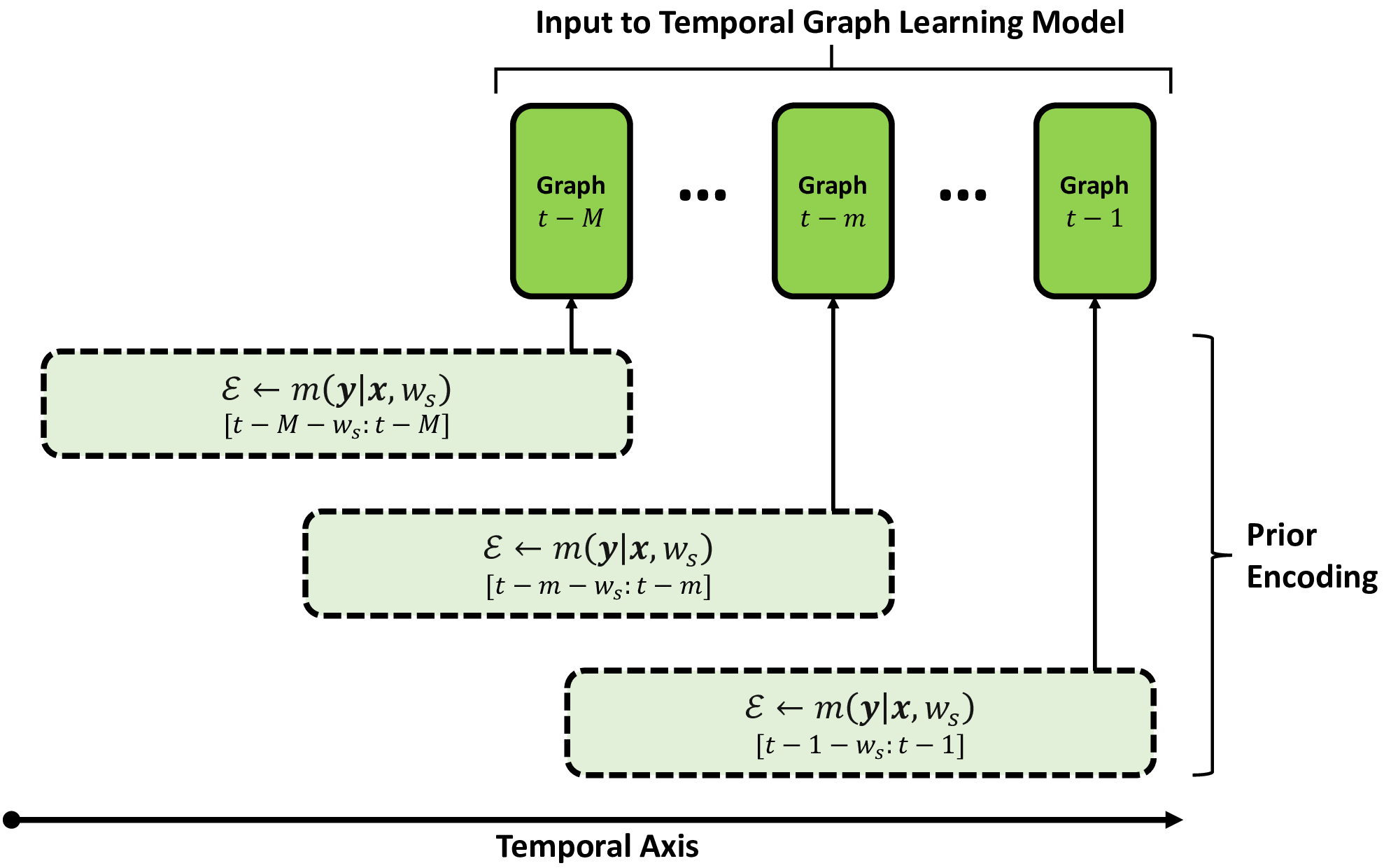
Figure 4. Sliding windows

5. Empirical Study

5.1. Data

To empirically test SSAR, we identify representative data sets that fit the definition of complex time series. We identify that financial time series are known to be highly stochastic, non-normal, and non-stationary (Alonso et al., 2021; Bastianin, 2020; Liu et al., 2023). In response, we source two financial time series data sets: (i) Inter-category variables and (ii) Intra-category variables. Inter- and Intra-category data sets exhaustively represent most financial time series. Henceforth, we refer to these data sets as Data Set 1 and 2, respectively. Both data sets have been sourced based on the largest international trading volumes—making them representative benchmarks that are directly applicable to practitioners. We detail the data sourcing and processing approach in the Appendix. Furthermore, we conduct extensive preliminary statistical tests in the Appendix to empirically prove the complexity of the time series.

5.2. Experiment Setting

We first apply SSAR to each data set. To examine the sensitivity to the hyperparameter $w_{s}$ we create SSAR $\forall w_{s}\in\textbf{{w}}_{s}:=\{$20, 30, 40, 50, 60, 70, 80}. The minimum size of 20 is chosen for the stability of information-theoretic measures. Then the data sets are split into train, validation, and test set—$0.5\times 0.7$, $0.5\times 0.3$, and $0.5$, respectively for Data Set 1, and $0.6$, $0.2$, and $0.2$, respectively for the Data Set 2. We set these splits to test splits that may occur in the real world.

We include five well-regarded baselines: (i) GRU, (ii) LSTM, (iii) Linear, (iv) NLinear, (v) DLinear, where (iii), (iv), (v) have shown to outperform all state-of-the-art transformer-based architectures. The $w_{s}$ for baselines corresponds to the temporal dimension size of the input vector. Next, to test the augmented representation, we select two well-known spatio-temporal GNNs—(i) (Li et al., 2017)’s Temporal Graph Diffusion Convolution Network (diffusion t-GCN), (ii) (Zhao et al., 2019)’s Temporal Graph Convolution Network (t-GCN). Notably, SSAR works with any downstream models that support spatio-temporal data with directed edges and dynamic weights. The number of compatible downstream models is very large. We arbitrarily let diffusion t-GCN be the downstream model for Data Set 1, and t-GCN for Data Set 2.

For ease of replication, we present the tensor operations of diffusion t-GCN for our representation in the Appendix. We do not diverge from the original method proposed by the authors for both downstream models. All experimental design choices, such as splits, downstream models, and sample sizes, were chosen a priori and were not changed after. Also, each empirical sample is independently trained via a random seed. I.e., no two test samples result from an inference of the same model $\hat{\theta}$.

The objective function $J$ is the mean squared error (MSE) of the prediction of $t$ given $[t\text{-}1:t\text{-}M]$. For a fair empirical study, we systematically tune hyperparameters $h\in\mathcal{H}\ \forall\langle w_{s}$, method, Data Set$\rangle$ in the train and validation set. I.e., the search over $\mathcal{H}$ is done algorithmically rather than human-tuning. Rigorous details of the training, validation, and inference process are provided in the Appendix with appropriate tables and pseudo-codes. We also have a discussion on computational complexity and scalability in the Appendix.

Table 1. Test Set Results (MSE)

Data Set 1
$w_{s}$	Pearson*	Spearman*	Kendall*	GC*	MI*	TE*	Constant‡	GRU†	LSTM†	Linear†	NLinear†	DLinear†
20	0.6621	0.6796	0.6646	0.7160	0.7209	0.7169	0.7519	0.8166	0.8154	0.8392	0.8775	0.8338
30	0.7149	0.6939	0.668	0.7237	0.7069	0.713	$\pm$	0.8154	0.8143	0.8355	0.8616	0.8370
40	0.7286	0.6698	0.7274	0.7361	0.7168	0.7055	0.0329	0.8161	0.8140	0.8376	0.8548	0.8368
50	0.7047	0.7082	0.7303	0.7237	0.6966	0.7411	($\pm 1\sigma$)	0.8150	0.8128	0.8388	0.8540	0.8426
60	0.8144	0.7205	0.7321	0.7077	0.7092	0.7079	—	0.8167	0.8165	0.8451	0.8545	0.8435
70	0.7200	0.7529	0.7289	0.7051	0.7207	0.7098	—	0.8154	0.8133	0.8468	0.8519	0.8519
80	0.7246	0.7162	0.7144	0.7173	0.7194	0.7038	—	0.8191	0.8141	0.8477	0.8535	0.8525
Data Set 2 ($\pm 1\sigma$)
$w_{s}$	Pearson*		Spearman*		Kendall*		GC*		MI*		TE*
20	$0.865570\pm 0.000001$		$0.869217\pm 0.000007$		$0.864707\pm 0.000000$		0.864074$\pm$0.000000		$0.867186\pm 0.000004$		$0.864379\pm 0.000000$
30	0.864372$\pm$0.000000		$0.865704\pm 0.000001$		$0.867756\pm 0.000004$		$0.864863\pm 0.000000$		$0.864390\pm 0.000000$		$0.865536\pm 0.000001$
40	$0.864416\pm 0.000000$		$0.864535\pm 0.000000$		$0.865272\pm 0.000000$		0.864074$\pm$0.000000		$0.864431\pm 0.000000$		$0.864167\pm 0.000000$
50	$0.865261\pm 0.000001$		$0.865146\pm 0.000000$		0.864197$\pm$0.000000		$0.865573\pm 0.000000$		$0.864614\pm 0.000000$		0.864126$\pm$0.000000
60	$0.864692\pm 0.000000$		$0.864584\pm 0.000000$		$0.866039\pm 0.000002$		$0.864528\pm 0.000000$		0.864271$\pm$0.000000		$0.864383\pm 0.000000$
70	$0.865183\pm 0.000001$		$0.864387\pm 0.000000$		$0.868527\pm 0.000004$		$0.867677\pm 0.000006$		0.864294$\pm$0.000000		$0.864967\pm 0.000001$
80	$0.864420\pm 0.000000$		$\textit{0.864216}\pm\textit{0.000000}$		$0.865633\pm 0.000002$		0.864100$\pm$0.000000		$0.866500\pm 0.000002$		$0.864747\pm 0.000000$
$w_{s}$	Constant‡		GRU†		LSTM†		Linear†		NLinear†		DLinear†
20	0.867078$\pm$0.000002		$1.073429\pm 0.001211$		$1.072995\pm 0.000342$		1.085739$\pm$0.001977		$1.141603\pm 0.000039$		$1.185543\pm 0.165922$
30	—		1.073149$\pm$0.000304		1.072988$\pm$0.000395		$1.088698\pm 0.002433$		$1.126325\pm 0.000044$		1.088895$\pm$0.000072
40	—		$1.073579\pm 0.000669$		$1.073082\pm 0.000406$		$1.092317\pm 0.001307$		$1.121533\pm 0.000045$		$1.094266\pm 0.005221$
50	—		$1.073659\pm 0.000514$		$1.073188\pm 0.000435$		$1.997715\pm 2.352422$		$1.120787\pm 0.000056$		$1.115725\pm 0.055661$
60	—		$1.075270\pm 0.001245$		$1.073747\pm 0.001143$		$1.100661\pm 0.006975$		$3.021245\pm 5.255515$		$4.500515\pm 9.036276$
70	—		$1.073497\pm 0.000584$		$1.073129\pm 0.000399$		$1.102755\pm 0.007010$		$1.120726\pm 0.000061$		$1.101896\pm 0.005430$
80	—		$1.073587\pm 0.000489$		$1.073001\pm 0.000308$		$1.127654\pm 0.019237$		1.120486$\pm$0.000057		$1.107615\pm 0.012696$

*SSAR: Non-Euclidean input-space, ^†Baseline: Euclidean input-space, ^‡Ablaftion
Bold represents the best result across row, and italicized represents the best result across column

5.3. Results and Ablation

We observe highly encouraging results, summarized in Figure 5 and Table 1. The following abbreviations are used for In Table 1, each column represents a method, and each row represents the $w_{s}$. The sample size for each $\langle$method, $w_{s}\rangle$ is one for Data Set 1 and 50 for Data Set 2. Note that the sample size for the Constant column does not conform to this pattern as Constant weighted edges are not associated with a $w_{s}$. However, to match the sample size for each approach, the Constant column presents the 7-sample mean$\pm 1\sigma$ results in Data Set 1. The Constant column in Data Set 2 presents a 50-sample result like every other result statistic.

The approaches are divided into (i) SSAR, ours, (ii) baselines, and (iii) ablation. The ablation approach, referred to as Constant, is where edge weights are set to a constant in place of a statistical measure. This allows us to examine the extent to which graphical structures are helpful, excluding the statistical measures. In Data Set 1, $\forall w_{s}$ SSAR achieved the best results. Notably, a significant improvement from baselines $\rightarrow$ ablation, and another significant improvement can be noticed from ablation $\rightarrow$ SSAR. Moreover, across 42-sample results for all six SSAR approaches and $w_{s}$, all 35-samples of baselines are beaten with a 100% beat rate.

In the case of Data Set 2, as each combination $\langle$method, $w_{s}\rangle$ is 50-sample, we have enough samples to compute the box-and-whisker plot in Figure 5. Each box-and-whisker aggregates across $w_{s}$, i.e., they each represent $7\cdot 50=350$ samples. We observe a dramatic improvement in accuracy across SSAR-based approaches. The box-and-whisker plot follows the standard, minimum, quartile-1, median, quartile-3, maximum value. We purposefully do not scale the x-axis to capture Linear, NLinear, and DLinear outliers. This would result in significant deterioration in legibility. An enlarged of Figure 5 is available in the Appendix.

Figure 5. Data Set 2 results (Box-and-Whisker, MSE)

6. Discussion

6.1. Statistical Analysis

In aggregate, $7\cdot 12$ (row $\cdot$ column) $=84$ random seed out-sample results are available for Data Set 1, and $7\cdot 11\cdot 50$ (row $\cdot$ column $\cdot$ sample-size) $=3850$ results are available for SSAR and baselines for Data Set 2. An additional 50 samples for the ablation leads to 3900 result samples for Data Set 2.

The statistical analysis is highly encouraging. First, we examine in aggregate whether the mean of SSARs beats the aggregate mean of the baselines. Data Set 1’s results are $0.7141\pm 0.0253$ (42-samples) and $0.8346\pm 0.0179$ (35-samples) for SSARs and baselines, respectively. The T-statistic is -23.9022 (P-val $\longrightarrow 0$). Data Set 2’s results are $0.8652\pm 0.0022$ (2100-samples) and $1.2740\pm 1.9097$ (1750-samples) for SSARs and baselines, respectively. The T-statistic is -9.8117 (P-val $\longrightarrow 0$).

We identify the best-performing baseline to assess SSAR more rigorously. In both the data sets, LSTM performs best when taking the mean value. In Data Set 1, SSARs against LSTM, the T-statistic is -10.3886 (P-val $\longrightarrow 0$). The T-statistic corresponding to Data Set 2 is -1,770 (P-val $\longrightarrow 0$). The $|$ T-statistic $|$ rises in Data Set 2 as the variance of LSTM is significantly lower than the baselines’ aggregate.

We have two ablation studies to examine our contribution further. The first study, the constant weighted edge case, has been previously introduced. In Data Set 1, the aggregate mean results going from baselines $\rightarrow$ Constant $\rightarrow$ SSARs is $0.8346\pm 0.0179\rightarrow 0.7519\pm 0.0329\rightarrow 0.7141\pm 0.0253$. This corresponds to a 9.91% reduction in MSE from baselines to Constant and a 5.02% reduction from Constant to SSARs. From baselines to SSARs, a 14.43% reduction is observed.

In Data Set 2, going from baselines $\rightarrow$ Constant $\rightarrow$ SSARs is $1.2740\pm 1.9097\rightarrow 0.8671\pm 0.0027\rightarrow 0.8652\pm 0.0022$. This corresponds to a 31.94% reduction in MSE from baselines to Constant and a 0.22% reduction from Constant to SSARs. From baselines to SSARs, a 32.09% reduction is observed. We further study the results at larger values of $w_{s}$, with corresponding statistical results in the Appendix. We find that the statistical significance remain robust.

The second ablation study further examines the observation of significant adverse outliers in the state-of-the-art methods—Linear, NLinear, and DLinear. For robustness, we examine whether the statistical results are robust even after removing adverse outliers of these models. The results are detailed in the Appendix—and the statistical findings remain unchanged. This observation of significant adverse outliers bodes poorly for the baselines and contrarily emphasizes the stability of our proposed approach. By examining the F-Test on baselines and SSARs, we observe an F-static of 764,534 and a corresponding one-tail F-Critical of 1.08 (P-val $\longrightarrow 0$). The evidence indicates a significant fall in the variance of SSARs.

Finally, we briefly discuss the implications of setting the $w_{s}$. Based on Figure 4, a naïve perspective would be assuming that SSARs improved performance is owed to implicitly encoding a larger $w_{s}$ since in agggregate its sliding window is $w_{s}+M$, while the baselines are only encoding $w_{s}$. However, if this was true, $\frac{\partial MSE_{test}}{\partial w_{s}}<0$. The empirical study shows no evidence of this phenomenon, as illustrated in Figure 6. On the contrary, there seems to be no meaningful relationship between $w_{s}$ and $MSE_{test}$ for the baselines. We present two histograms that summarize $p(min(MSE_{test})|w_{s},B\lor S)$, where $B\lor S$ denotes a boolean with some abuse of notation—true: Baseline, false: SSAR).

Figure 6. Histogram of minimum MSE given $w_{s}$ (both data sets)

6.2. Theoretical Implications

At first glance, a questionable result is an improvement in performance in the Constant ablation case. Based on the theoretical discussion provided by (Koh et al., 2023), we show that SSAR is not only helpful in modeling the shifting underlying distribution but also implicitly smooths highly stochastic data. We first summarize these effects visually in Figure 7. (Koh et al., 2023) shows that when the causal structure is very high-dimensional and therefore highly stochastic, augmenting the training data via smoothing techniques is helpful when noise-to-signal is high. The authors use exponential moving averages to smooth the input and target space. We show that SSAR paired with a temporal graph learning algorithm implicitly makes the same augmentations—explaining the improved performance in the Constant ablation case.

Temporal weighted graph learning algorithms that perform node prediction fundamentally learn to aggregate (message pass) the weight(s) and node(s) closest to each node. Afterwards, this new encoding is fed into some neural network with a temporal encoding (e.g., RNNs, Transformers). Here, $w(\cdot)$ denotes weights of edges, while $\theta$ denotes weights parameterizing the learning system. In its theoretically simplest form, without loss of generality, suppose it aggregates the weights of edges incident to the node, then,

$$\forall nodes,\ \hat{n}_{i}:=n_{i}+\left[\sum_{e\in\mathcal{I}_{i}}w(e)\theta_{i}(e)\right],$$

where $\hat{n}_{i}$ is the post-encoding node embedding, $\mathcal{I}_{i}$ is the set of edges incident to $n_{i}$, and $\theta_{i}$ is the learned weight parameter. First, we know that $w(\cdot)\geq 0$, and it is safe to assume that $\sum_{e}w(e)>0$ for both the Constant and SSAR case. Then, whether $\hat{n}_{i}>n_{i}$ or $\hat{n}_{i}<n_{i}$, and magnitude $|\hat{n}_{i}-n_{i}|$ is only dependant on parameter $\theta_{i}(e)$. Meaning, $\theta_{i}(e)$ can learn to de-noise the highly stochastic data. De-noising high noise-to-signal time series has resulted in dramatically improved results, as seen in (Koh et al., 2023). Essentially, as long as the Constant weight,

$$w(\cdot):=c\in\mathbb{R}_{\neq 0},$$

$\Rightarrow\theta_{i}$ can implicitly learn to de-noise the input and target space, resulting in improved out-sample performance. This explains why adding no statistical-space prior, but a simple augmented representation with fixed $w(\cdot):=c>0$, $\forall w(\cdot)$ resulted in improved performance.

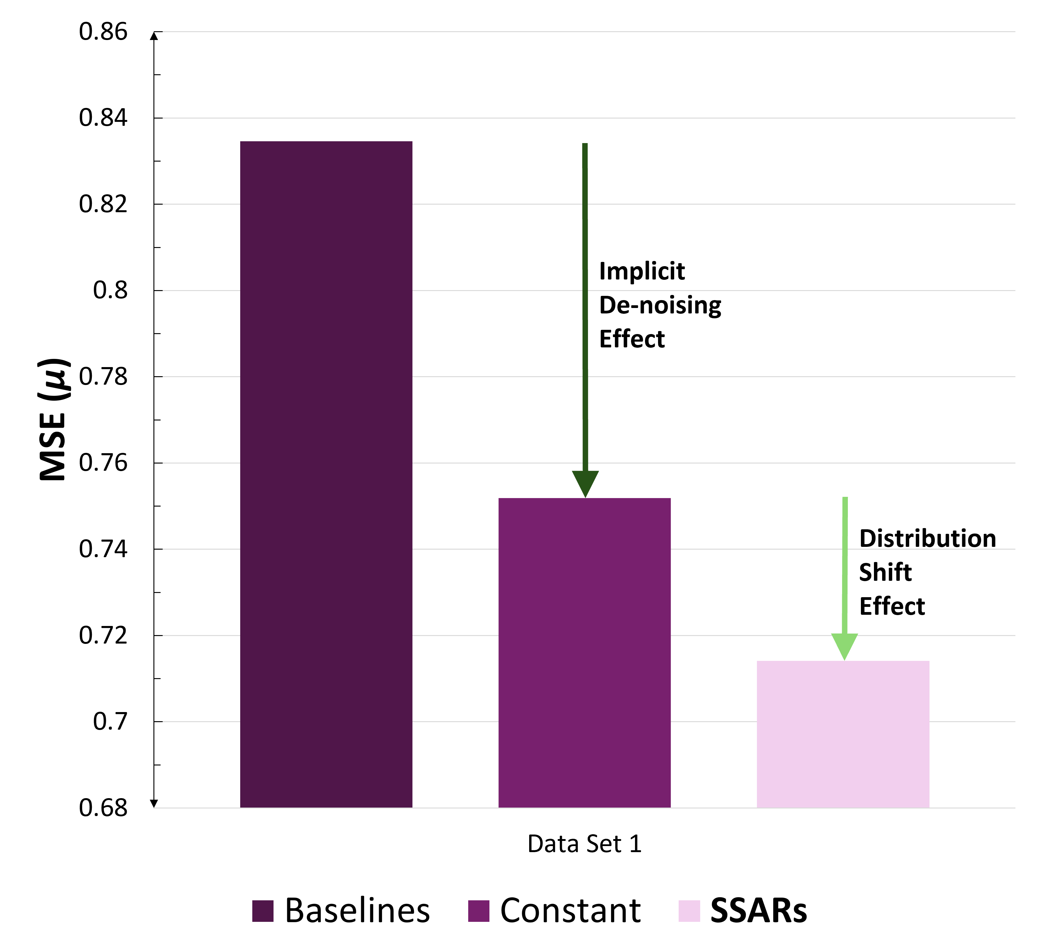
Figure 7. Two effects

This implicit de-noising partially explains the superior performance of SSAR. The remaining improvement is due to approximating Equation (8) via Equation (9). In short, SSAR can be decomposed into two effects: (i) SS: statistical-space encoding, which tracks the underlying distribution shift, and (ii) AR: augmented representation, which allows for a learnable function approximator to implicitly de-noise the stochastic data.

However, unlike the clear-cut effects shown in Figure 7, decomposing SSAR into SS and AR is challenging. As seen in Equation (13), $\theta_{i}(e)$ could not only learn to de-noise the data but also implicitly learn the $\textbf{{r}}\leftarrow r_{\theta_{r}}(\textbf{{y}}^{t}|\hat{\textbf{{x}}}))$ in Equation (5). Also when providng prior $p(\theta)$ in Equation (4) via $\textbf{{e}}^{t-M}\in\mathcal{E}$, in which it passed through Equation (13), there is no obvious way of decomposing the two effects. Therefore, despite our ablation study’s role in helping us understand the mechanisms behind SSAR’s improved performance, it should not be taken as a rigorous methodology to quantify the two effects.

6.3. Future Works

Our work, which compares SSAR and Euclidean input-space-based state-of-the-art models, can be viewed as two ends of the extreme. Euclidean input-space-based models must learn the underlying non-stationary distribution implicitly, while SSAR takes a more deliberate approach.

SSAR explicitly provides a statistical-space approximation $\forall t$, resulting in (i) allowing the neural network to use an approximated regime-vector, and further learn the distribution shift, and (ii) bootstrap the neural network with priors, given that our data is limited. However, in cases where we have access to $\mathcal{D}\sim p(\cdot)$, or $|\mathcal{D}|$ is already sufficiently large, we can hypothesize that a learned statistical space may be beneficial. I.e., implement Equation (5) instead of Equation (9). In this case, the statistical space could be learned implicitly via $\theta:\cdot\cdot\cdot\times\langle n_{i}\rightarrow n_{j}\rangle\times\cdot\cdot\cdot\mapsto\mathbb{R}$, $i\neq j$ where edge weights are initialized $w^{init}(e):\neq 0$, in Equation (13). Under the Bayesian view in Equation (4), this would correspond to the prior being a uniform distribution, $p(\theta):=U(\cdot)$. Contrarily, the statistical space could be learned explicitly where the weights of the edges are learned explicitly, $w_{\theta}:\cdot\cdot\cdot\times\langle n_{i}\rightarrow n_{j}\rangle\times\cdot\cdot\cdot\mapsto\mathbb{R}_{\geq 0}$, $i\neq j$. This would closely mimic the attention mechanism in transformers.

We encourage future research to explore these middle-ground approaches within the solution space spectrum presented here. A more nuanced study could theoretically and empirically study which method in the spectrum is most ideal under specific degrees of access to $p(\cdot)$, equivalently, amount of data $\mathcal{D}$ available.

Appendix A Assumption: $\hat{\textbf{{x}}}_{[,:]}:=\textbf{{y}}_{[,:]}$

The assumption that the input-space features are equivalent to the output-space features is highly reasonable. Essentially, when training to predict y, since $|\mathcal{D}|\gg 0\Rightarrow\textbf{{y}}_{[:,]}\gg 0\ \therefore\exists\hat{\textbf{{x}}}_{[:,]}\gg 0$. Even if $\hat{\textbf{{x}}}_{[,:]}\neq\textbf{{y}}_{[,:]}$, the method and implications presented in this work hold with trivial modifications in the learning system.

Appendix B Data Source

Table 2. Data Set 1 Description

Variable	Abbreviation	Category
SPDR Gold Trust	GLD	Commodity
U.S. Oil Fund	USO	Commodity
U.S. Dollar Index	USD	Currency
U.S. IG Corporate Bond	LQD	Fixed Income
3M Treasury Yield	3M	Interest Rate
2Y Treasury Yield	2Y	Interest Rate
10Y Treasury Yield	10Y	Interest Rate
Fed Funds Effective Rate	FFEOR	Interest Rate
10Y-3M Spread	10Y-3M	Rate Spread
10Y-2Y Spread	10Y-2Y	Rate Spread
U.S. Real Estate	IYR	Real Estate
CBOE Volatility Index	VIX	Risk
Bull-Bear Spread	BULL_BEAR_SPREAD	Sentiment

Table 3. Data Set 2 Description

Variable	Category
Wheat Futures	Commodity
Corn Futures	Commodity
Copper Futures	Commodity
Silver Futures	Commodity
Gold Futures	Commodity
Platinum Futures	Commodity
Crude Oil Futures	Commodity
Heating Oil Futures	Commodity

We use two representative data sets for financial markets. The first is an array of major macroeconomic exchange-traded funds (ETFs) and variables, available in Table 2. These variables are representative as they have been chosen based on the largest worldwide trading volumes. This data set examines the effectiveness of our approach across many financial categories (inter-asset-class). The second data set is an array of major commodity futures available in Table 3. Again, these features are chosen beforehand based on the largest worldwide trading volume. This data set examines the effectiveness of our approach within a financial category (intra-asset-class)—commodity futures market.

Both data sets are easily attainable via public sources. However, we source the data from S&P Capital IQ and Bloomberg for high-quality data that is not adjusted later—to concretely prevent any look-ahead bias. The Bull-Bear Spread is sourced separately from the Investor Sentiment Index of the American Association of Individual Investors (AAII).

The initial time step is set to the date where $\exists$ valid data points $\forall$ variable. Data Set 1’s date spans from 2006-04-11 to 2022-07-08 in daily units. Data Set 2’s date spans from 1990-01-01 to 2023-06-26 in daily units.

Appendix C DATA PROCESSING

The only data processing done from raw data is transforming price data into return (change) data, and pre-processing non-available (nan) data points. We transform market variables to log return, as typical practice in the financial domain. Log return is used instead of regular difference as log allows for computational convenience. Other data points are transformed to the regular difference approach as their data points are much smaller in magnitude, and require higher levels of precision. The pseudo-code for the data processing is available in Algorithm 2.

1:Input: $\textbf{{D}}_{raw}$

2:Output: $\textbf{{D}}_{processed}$

3:Function DataProcess($\textbf{{D}}_{raw}$):

4:$init\ \ \textbf{{D}}_{processed}$

5:$\mathcal{F}\longleftarrow\textbf{{D}}_{raw}.get\_feature\_set()$

6:

7:for $f\in\mathcal{F}$ do

8:     if $f$ is $MarketVariable$ then

9:         $\forall\textbf{{D}}_{processed}[f].datapoint[i]\longleftarrow log(\textbf{{D}}_{raw}[f].datapoint[i]/\textbf{{D}}_{raw}[f].datapoint[i-1])$

10:     else if $f.datapoints\neq nan$ then

11:         $\forall\textbf{{D}}_{processed}[f].datapoint[i]\longleftarrow\textbf{{D}}_{raw}[f].datapoint[i]-\textbf{{D}}_{raw}[f].datapoint[i-1]$

12:     else

13:         $\forall\textbf{{D}}_{processed}[f].datapoint[i]\longleftarrow\textbf{{D}}_{raw}[f].datapoint[i]-\textbf{{D}}_{raw}[f].datapoint[most\_recent\_non\_nan\_i<i]$

14:     end if

15:end for

16:

17:$\textbf{{D}}_{processed}[\mathcal{F}].datapoint[0].drop\_timestep()$

18:return $\textbf{{D}}_{processed}$

19:End Function

Algorithm 2 Data Process

Appendix D Computing statistical dependencies

Given $\textbf{{n}}_{i}:=\{i_{t-1},...,i_{t-1-w_{s}}\}$ and $\textbf{{n}}_{j}:=\{j_{t-1},...,j_{t-1-w_{s}}\}$, the six measures are computed as follows. We remove the superscript $t$ for improved legibility and let $\rho_{\textbf{{n}}_{i},\textbf{{n}}_{j}}$, $\rho_{r_{\textbf{{n}}_{i}},r_{\textbf{{n}}_{j}}}$, $\tau_{r_{\textbf{{n}}_{i}},r_{\textbf{{n}}_{j}}}$, denotes Pearson correlation, Spearman rank correlation, and Kendell rank correlation, respectively. $r_{\textbf{{n}}_{i}}$ denotes rank for time series $\textbf{{n}}_{i}$. Then, define each correlation as (15), (16), and (17).

$$\rho_{\textbf{{n}}_{i},\textbf{{n}}_{j}}:=\frac{\Sigma_{t}(n_{i}^{t}-\bar{\textbf{{n}}_{i}})(n_{j}^{t}-\bar{\textbf{{n}}_{j}})}{\sqrt{\Sigma_{t}(n_{i}^{t}-\bar{\textbf{{n}}_{i}})^{2}}\sqrt{\Sigma_{t}(n_{j}^{t}-\bar{\textbf{{n}}_{j}})^{2}}},$$

$$\rho_{r_{\textbf{{n}}_{i}},r_{\textbf{{n}}_{j}}}:=\frac{cov(r_{\textbf{{n}}_{i}},r_{\textbf{{n}}_{j}})}{\sigma_{r_{\textbf{{n}}_{i}}}\sigma_{r_{\textbf{{n}}_{j}}}},$$

$$\tau_{r_{\textbf{{n}}_{i}},r_{\textbf{{n}}_{j}}}:=\frac{c-d}{\frac{1}{2}w_{s}(w_{s}-1)},$$

where $\bar{\textbf{{n}}_{i}}$ denotes the mean of series $\textbf{{n}}_{i}$, $c$ is the number of concordant pairs, and $d$ is the number of discordant pairs. A pair $\langle n^{t,a}_{i},n^{t,a}_{j}\rangle$,$\langle n^{t,b}_{i},n^{t,b}_{j}\rangle$ is concordant if the ranks for both elements agree in their order: $(n^{t,a}_{i}-n^{t,b}_{i})(n^{t,a}_{j}-n^{t,b}_{j})>0$, and discordant if they disagree $(n^{t,a}_{i}-n^{t,b}_{i})(n^{t,a}_{j}-n^{t,b}_{j})<0$.

We used Granger causality (Granger, 1969) based on Geweke’s method (Geweke, 1982). Geweke’s Granger causality (GC) is a frequency-domain approach to Granger causality. Geweke’s Granger causality from $\textbf{{n}}_{i}$ to $\textbf{{n}}_{j}$ is computed by:

$$GC_{\textbf{{n}}_{i}\longrightarrow\textbf{{n}}_{j}}:=\ln\left(\frac{S_{\textit{n}_{j}\textit{n}_{j}}(f)}{S_{\textit{n}_{j}\textit{n}_{j}|\textit{n}_{i}}(f)}\right),$$

where $S_{\textit{n}_{j}\textit{n}_{j}}(f)$ is the spectral density of $\textbf{{n}}_{j}$ and $S_{\textit{n}_{j}\textit{n}_{j}|\textit{n}_{i}}(f)$ is the spectral density of $\textbf{{n}}_{j}$ given $\textbf{{n}}_{i}$. We use Welch’s method to estimate spectral density as it improves over periodograms in estimating the power spectral density of a signal (Welch, 1967).

We used two information-theoretic measures: Mutual information and Transfer entropy. Mutual information (MI) represents the shared information between two variables, indicating their statistical interdependence (Shannon, 1948). In information theory, the behavior of system $\textbf{{n}}_{i}$ can be characterized by the probability distribution $p(\textbf{{n}}_{i})$ or $\log p(\textbf{{n}}_{i})$. This measure is equivalent to the Pearson correlation coefficient if both have a normal distribution. To compute MI between two variables, we need to know the information entropy, which is formulated as follows:

$$H(\textbf{{n}}_{i}):=-\sum_{\textit{n}_{i}\in\textbf{{n}}_{i}}p(\textit{n}_{i})\log_{2}p(\textit{n}_{i}).$$

Shannon entropy quantifies the information required to select random values from a discrete distribution. The joint (information) entropy can be expressed as:

$$H(\textbf{{n}}_{i},\textbf{{n}}_{j}):=-\sum_{\textit{n}_{i}\in\textbf{{n}}_{i},\textit{n}_{j}\in\textbf{{n}}_{j}}p(\textit{n}_{i},\textit{n}_{j})\log_{2}p(\textit{n}_{i},\textit{n}_{j}).$$

Finally, we can define MI as the quantity of identifying the interaction between subsystems.

$$MI(\textbf{{n}}_{i},\textbf{{n}}_{j}):=H(\textbf{{n}}_{i})+H(\textbf{{n}}_{j})-H(\textbf{{n}}_{i},\textbf{{n}}_{j}).$$

Following Kvålseth (2017), we use normalized MI (NMI) with range [0, 1] to ensure consistency across measures. The computation is as follows:

$$NMI(\textbf{{n}}_{i},\textbf{{n}}_{j}):=\frac{MI(\textbf{{n}}_{i};\textbf{{n}}_{j})}{\min(H(\textbf{{n}}_{i}),H(\textbf{{n}}_{j}))}.$$

Transfer entropy (TE) is a non-parametric metric leveraging Shannon’s entropy, quantifying the amount of information transfer between two variables (Schreiber, 2000). Based on conditional MI in Equation (23), we can define the general form of $(k,l)$-history TE between two sequences $\textbf{{n}}_{i}$ and $\textbf{{n}}_{j}$ for $\textbf{{n}}_{i,t}^{(k)}=(\textbf{{n}}_{i,t},.,\textbf{{n}}_{i,t-k+1})$ and $\textbf{{n}}_{j,t}^{(l)}=(\textbf{{n}}_{j,t},.,\textbf{{n}}_{j,t-l+1})$. It is computed as Equation (24):

$$H(\textbf{{n}}_{j}|\textbf{{n}}_{i}):=-\sum_{\textit{n}_{j}\in\textbf{{n}}_{j},\textit{n}_{i}\in\textbf{{n}}_{i}}p(\textit{n}_{i},\textit{n}_{j})\log_{2}\frac{p(\textit{n}_{i},\textit{n}_{j})}{p(\textit{n}_{i})}.$$

$$TE_{\textbf{{n}}_{i,t}\longrightarrow\textbf{{n}}_{j,t}}^{(k,l)}(t):=$$

$$\sum_{\Omega}p(\textit{n}_{j,t+1},\textit{n}_{i,t}^{(k)},\textit{n}_{j,t}^{(l)})\log_{2}\frac{p(\textit{n}_{j,t+1}|\textit{n}_{i,t}^{(k)},\textit{n}_{j,t}^{(l)})}{p(\textit{n}_{j,t+1}|\textit{n}_{j,t}^{(l)})},$$

where $\Omega:=\{\textit{n}_{j,t+1},\textit{n}_{i,t}^{(k)},\textit{n}_{j,t}^{(l)}\}$, which represents the possible sets of those three values. $TE_{\textbf{{n}}_{i,t}\longrightarrow\textbf{{n}}_{j,t}}^{(k,l)}(t)$ is the information about the future state of $\textbf{{n}}_{j,t}$ which is retrieved by subtracting information retrieved from only $\textbf{{n}}_{j,t}^{(l)}$, and from information gathered from $\textbf{{n}}_{i,t}^{(k)}$ and $\textbf{{n}}_{j,t}^{(l)}$. We set $k$ and $l$ to 1. Under these conditions, the equation for TE with $(1,1)$-history can be computed as

$$TE_{\textbf{{n}}_{i,t}\longrightarrow\textbf{{n}}_{j,t}}^{(1,1)}(t)=$$

$$\sum_{\Omega}p(\textit{n}_{j,t+1},\textit{n}_{j,t},\textit{n}_{i,t})\log_{2}\frac{p(\textit{n}_{j,t+1},\textit{n}_{i,t},\textit{n}_{j,t})p(\textit{n}_{j,t})}{p(\textit{n}_{j,t+1},\textit{n}_{j,t})p(\textit{n}_{i,t},\textit{n}_{j,t})},$$

where $\Omega=\{\textbf{{n}}_{j,t+1},\textbf{{n}}_{i,t},\textbf{{n}}_{j,t}\}$.

This measure can be perceived as conditional mutual information, considering a variable’s influence as a condition. Also, analogous to the established relationship between the Pearson correlation coefficient and mutual information, an equivalent association can be identified when the two variables comply with the premises of normal distribution (Barnett et al., 2009). TE measures information flow via uncertainty reduction. ”TE from $Y$ to $X$,” translates to the extent $Y$ clarifies the future of $X$ beyond what $X$ can clarify about its own future. Conditional entropy quantifies the requisite information to derive the outcome of a random variable $X$, given that the value of another random variable $Y$ is known. It is computed as (Barnett et al., 2013):

Appendix E Descriptive Statistics and Statistical Properties

Tables 4, 5, 6, and 7 summarize the time series’s descriptive statistics and statistical property tests. The means and standard deviations clearly indicate the high noise-to-signal ratio—$\mu\approx 0$ and $\sigma>>|\mu|$.

All eight normality statistics strongly indicate non-normality. Most features are non-auto-correlated, and all features are non-stationary. “***” denotes rejection of the null hypothesis of statistical tests at the 0.01 level of significance, “**” at the 0.05 level, and “*” at the 0.1 level.

Table 4. Descriptive Statistics (Data Set 1)

Statistic	GLD	USO	USD	LQD	3M	2Y	10Y
Mean, $\mu$	0.0003	-0.0003	0.0001	0	-0.0002	-0.0002	-0.0001
Standard deviation, $\sigma$	0.0156	0.0156	0.0156	0.0156	0.0156	0.0156	0.0156
Skewness	-0.334	-1.1831	-0.2533	-0.5572	-0.8177	-0.0971	-0.1188
Kurtosis	6.3099	14.8191	4.0016	67.8462	77.2192	11.4556	3.507
$Q_{0}$	-0.1255	-0.1912	-0.1394	-0.2696	-0.2663	-0.1529	-0.1432
$Q_{1}$	-0.0071	-0.0078	-0.0083	-0.006	-0.0033	-0.0068	-0.0084
$Q_{2}$	0.0007	0.0005	0.0003	0.0009	0	0	0
$Q_{3}$	0.0083	0.0079	0.0088	0.0066	0.0033	0.0068	0.0084
$Q_{4}$	0.1461	0.101	0.0883	0.263	0.2498	0.1291	0.0814
Statistic	FFEOR	10Y-3M	10Y-2Y	IYR	VIX	BULL_BEAR_SPREAD
Mean, $\mu$	-0.0002	0	0	0.0001	0	-0.0001
Standard deviation, $\sigma$	0.0156	0.0156	0.0156	0.0156	0.0156	0.0156
Skewness	-0.4796	0.3396	-0.0493	-0.6986	1.0469	-0.0633
Kurtosis	88.5722	13.4647	3.6125	18.3742	5.9128	0.317
$Q_{0}$	-0.2175	-0.1226	-0.1122	-0.1889	-0.0705	-0.0538
$Q_{1}$	0	-0.0074	-0.008	-0.0051	-0.0088	-0.0102
$Q_{2}$	0	0	0	0.0006	-0.0013	0.0002
$Q_{3}$	0	0.0074	0.008	0.0059	0.0071	0.0107
$Q_{4}$	0.2404	0.1744	0.0841	0.1238	0.1546	0.0561

Table 5. Statistical Tests (Data Set 1)

Test	Type	GLD	USO	USD	LQD	3M
Shapiro-Wilk	Normality	0.9412***	0.9106***	0.9674***	0.7205***	0.5102***
D’Agostino K-squared	Normality	611.7238***	1504.0233***	421.8482***	1671.8988***	1886.876***
Lilliefors	Normality	0.0711***	0.0694***	0.0494***	0.1092***	0.2776***
Jarque-Bera	Normality	6834.6006***	38241.7946***	2761.1181***	781940.6002***	1013102.2671***
Kolmogorov–Smirnov	Normality	0.4771***	0.4764***	0.4761***	0.4783***	0.4758***
Anderson-Darling	Normality	44.797***	49.312***	22.4254***	143.6918***	527.6964***
Cramér–von Mises	Normality	327.3755***	327.6465***	327.0075***	329.5083***	332.1592***
Omnibus	Normality	611.7238***	1504.0233***	421.8482***	1671.8988***	1886.876***
Bruesch-Godfrey (5d)	Autocorrelation	0.6548	1.8472	1.8339	1.7377	15.8475***
Ljung-Box (5d)	Autocorrelation	0.6468	1.8631	1.8317	1.7303	16.0909***
Augmented Dicky-Fuller	Stationarity	-64.3747***	-9.0878***	-63.4386***	-12.0401***	-10.498***
Zivot-Andrews	Stationarity	-64.4844***	-9.5335***	-63.5556***	-12.7633***	-11.4003***
Phillips-Perron	Stationarity	-64.7455***	-64.5927***	-63.4453***	-64.147***	-52.8798***
Statistic	Type	2Y	10Y	FFEOR	10Y-3M	10Y-2Y
Shapiro-Wilk	Normality	0.8738***	0.9706***	0.3504***	0.8904***	0.9594***
D’Agostino K-squared	Normality	783.0878***	347.5444***	1720.7889***	918.375***	348.7078***
Lilliefors	Normality	0.1361***	0.0678***	0.3541***	0.09***	0.0969***
Jarque-Bera	Normality	1332463.2869***	30862.2392***	2216.2285***	22288.2101***	2096.6655***
Kolmogorov–Smirnov	Normality	0.474***	0.4772***	0.4764***	0.4753***	0.4765***
Anderson-Darling	Normality	116.837***	22.8665***	894.9531***	60.1568***	38.2637***
Cramér–von Mises	Normality	328.2026***	326.93***	334.2273***	327.8856***	327.0914***
Omnibus	Normality	783.0878***	347.5444***	1720.7889***	918.375***	348.7078***
Bruesch-Godfrey (5d)	Autocorrelation	19.2069***	1.947	44.1751***	20.4973***	4.4516
Ljung-Box (5d)	Autocorrelation	18.6156***	1.9235	45.6069***	20.3085***	4.4324
Augmented Dicky-Fuller	Stationarity	-9.294***	-13.635***	-11.2644***	-9.8368***	-47.7222***
Zivot-Andrews	Stationarity	-10.9044***	-47.8802***	-10.7794***	-14.2945***	-11.688***
Phillips-Perron	Stationarity	-67.0877***	-64.7715***	-74.8074***	-59.8906***	-63.198***
Test	Type	IYR	VIX	BULL_BEAR_SPREAD
Shapiro-Wilk	Normality	0.8043***	0.936***	0.9975***
D’Agostino K-squared	Normality	1247.5579***	1034.8942***	15.9253***
Lilliefors	Normality	0.1303***	0.0785***	0.0166***
Jarque-Bera	Normality	57660.7643***	6680.5179***	19.6321***
Kolmogorov–Smirnov	Normality	0.4713***	0.4784***	0.4797***
Anderson-Darling	Normality	175.1698***	49.7635***	1.8623***
Cramér–von Mises	Normality	328.9962***	327.3539***	326.375***
Omnibus	Normality	1247.5579***	1034.8942***	15.9253***
Bruesch-Godfrey (5d)	Autocorrelation	5.7178	8.9025	90.8848***
Ljung-Box (5d)	Autocorrelation	5.7007	8.969	84.6422***
Augmented Dicky-Fuller	Stationarity	-11.7587***	-26.8927***	-16.958***
Zivot-Andrews	Stationarity	-13.299***	-26.9875***	-16.9997***
Phillips-Perron	Stationarity	-76.062***	-75.9458***	-17.7063***

Table 6. Descriptive Statistics (Data Set 2)

Test	Wheat	Corn	Copper	Silver	Gold	Platinum	Crude Oil	Heating Oil
Mean	0.0001	0.0001	0.0002	0.0002	0.0002	0.0001	0.0002	0.0001
Standard deviation	0.0196	0.0171	0.0164	0.0184	0.0102	0.0149	0.0259	0.0239
Skewness	-0.2386	-1.1802	-0.2838	-0.7025	-0.2434	-0.9835	-0.4843	-1.3415
Kurtosis	12.7754	20.1985	4.392	7.324	7.4048	17.7037	20.1242	17.3938
$Q_{0}$	-0.2861	-0.2762	-0.1171	-0.1955	-0.0982	-0.2719	-0.4005	-0.3909
$Q_{1}$	-0.0111	-0.0085	-0.0083	-0.0079	-0.0044	-0.074	-0.012	-0.0114
$Q_{2}$	0	0	0	0.0005	0.0002	0.0005	0.0006	0.0006
$Q_{3}$	0.0107	0.0089	0.0088	0.0091	0.0052	0.008	0.0129	0.0124
$Q_{4}$	0.233	0.1276	0.1164	0.122	0.0889	0.1272	0.3196	0.1399

Table 7. Statistical Tests (Data Set 2)

Test	Type	Wheat	Corn	Copper	Silver
Shapiro-Wilk	Normality	0.9389***	0.9174***	0.9552***	0.9241***
D’Agostino K-squared	Normality	1752.8365***	3332.3089***	944.7587***	1783.9423***
Lilliefors	Normality	0.0455***	0.0637***	0.0542***	0.0845***
Jarque-Bera	Normality	57149.8899***	144614.381***	6856.3562***	19445.8744***
Kolmogorov–Smirnov	Normality	0.472***	0.4738***	0.4748***	0.4723***
Anderson-Darling	Normality	49.7856***	89.5722***	67.6838***	127.1812***
Cramér–von Mises	Normality	666.284***	671.1711***	671.5948***	669.1654***
Omnibus	Normality	1752.8365***	3332.3089***	944.7587***	1783.9423***
Bruesch-Godfrey (5d)	Autocorrelation	3.1197	1.0919	0.8877	7.1119
Ljung-Box (5d)	Autocorrelation	3.0741	1.0829	0.8948	7.1953
Augmented Dicky-Fuller	Stationarity	-20.5887***	-88.3374***	-24.3989***	-30.846***
Zivot-Andrews	Stationarity	-20.7714***	-88.3823***	-24.5412***	-31.0458***
Phillips-Perron	Stationarity	-92.3386***	-88.3095***	-96.4925***	-93.9752***
Test	Type	Gold	Platinum	Crude Oil	Heating Oil
Shapiro-Wilk	Normality	0.9289***	0.928***	0.8887***	0.9089***
D’Agostino K-squared	Normality	1305.4712***	2923.7298***	2357.3219***	3450.6279***
Lilliefors	Normality	0.0803***	0.0631***	0.0715***	0.0691***
Jarque-Bera	Normality	19253.8825***	110951.6968***	141944.7626***	108313.6979***
Kolmogorov–Smirnov	Normality	0.4826***	0.4781***	0.4646***	0.4664***
Anderson-Darling	Normality	114.6614***	80.9492***	120.7886***	97.4767***
Cramér–von Mises	Normality	682.8616***	674.6513***	657.7334***	660.199***
Omnibus	Normality	1305.4712***	2923.7298***	2357.3219***	3450.6279***
Bruesch-Godfrey (5d)	Autocorrelation	3.6289	7.7309	16.502***	5.2739
Ljung-Box (5d)	Autocorrelation	3.5897	7.73	16.9965***	5.3533
Augmented Dicky-Fuller	Stationarity	-36.1101***	-15.4566***	-15.5826***	-24.3777***
Zivot-Andrews	Stationarity	-36.3411***	-15.801***	-15.7147***	-24.4921***
Phillips-Perron	Stationarity	-92.7712***	-89.3201***	-92.1408***	-93.4847***

Appendix F GRAPH DIFFUSION CONVOLUTIONAL NETWORK

We implement a t-GCN powered by diffusion convolutional recurrent neural networks (DCRNN) to learn SSAR’s spatial and temporal dependency structure (Li et al., 2018). DCRNN shows state-of-the-art performance in modeling traffic dynamics with a spatial and temporal dimension—represented graphically.

The graph signal $\mathcal{X}\in\mathbb{R}^{N\times 1}$ as each node has a single feature. With $\mathcal{X}^{t}$ representing the signal observed at time $t$, the diffusion t-GCN learns a function $g(\cdot)$:

$$[\mathcal{X}^{t-M},\ldots,\mathcal{X}^{t-1};\mathcal{G}]\xrightarrow{g(\cdot)}[\mathcal{X}^{t}].$$

The diffusion process explicitly captures the spatial dimension and its stochastic features. The diffusion process in generative modeling works by encoding information via increasing noise through a Markov process while decoding information via reversing the noise process (Rombach et al., 2022). The diffusion mechanism here is characterized by a random walk on $\mathcal{G}$ with restart probability $\alpha\in[0,1]$, and state transition matrix $\textbf{{D}}_{O}^{-1}\mathcal{W}$, where $\textbf{{D}}_{O}=diag(\mathcal{W}\textbf{1})$ is the out-degree diagonal matrix, and $\textbf{1}\in\mathbb{R}^{N}$ is the all-one vector. The stationary distribution $\mathcal{P}\in\mathbb{R}^{N\times N}$ of the diffusion process can be computed via the closed form:

$$\mathcal{P}:=\sum_{k=0}^{K=\infty}\alpha(1-\alpha)^{k}(\textbf{{D}}_{O}^{-1}\mathcal{W})^{k}.$$

After sufficient time steps, as represented by the summation to infinity, the Markov process converges to $\mathcal{P}$. The intuition is as follows. $\mathcal{P}_{i,:}\in\mathbb{R}^{N}$ represents the diffusion probability from $n_{i}$, i.e., it quantifies the proximity with respect to the node. $k$ denotes the diffusion steps, and $K$ is typically set to a finite natural number as each step is analogous to the filter size in convolution.

As a result, the diffusion convolution over our $\mathcal{X}$ and a filter $f_{\theta}$ is described by:

$$\mathcal{X}_{:,1}\star_{G}f_{\theta}:=\sum_{k=0}^{K-1}(\theta_{k,1}(\textbf{{D}}_{O}^{-1}\mathcal{W})^{k}+\theta_{k,2}(\textbf{{D}}_{I}^{-1}\mathcal{W}^{T})^{k})\mathcal{X}_{:,1},$$

where $\theta\in\mathbb{R}^{K\times 2}$ are filter parameters and $\textbf{{D}}_{O}^{-1}\mathcal{W}$, $\textbf{{D}}_{I}^{-1}\mathcal{W}^{T}$ are the diffusion process transition matrices with the latter representing the reverse process. A diffusion convolution layer within a neural network architecture would map the signal’s feature size to an output of dimension $\mathcal{Q}$. As we are working with a single feature, we denote a parameter tensor as $\Theta\in\mathbb{R}^{Q\times 1\times K\times 2}=[\theta]_{q,1}$. The parameters for the $q$th output is $\Theta_{q,1}\in\mathbb{R}^{K\times 2}$. In short, the diffusion convolutional layer is described as:

$$\mathcal{H}_{:,q}:=a(\mathcal{X}_{:,1}\star_{G}f_{\Theta_{q,1,:,:}}),\quad for\ q\in\{1,\ldots,\mathcal{Q}\}.$$

Where input $\mathcal{X}\in\mathbb{R}^{N}$ is mapped to output $\mathcal{H}\in\mathbb{R}^{N\times\mathcal{Q}}$, and $a(\cdot)$ is an activation function. With this GCN structure, we can train the network parameters via stochastic gradient descent.

Appendix G DIFFUSION CONVOLUTIONAL GATED RECURRENT UNIT

Next, the temporal dimension is modeled via a GRU, a variant of RNNs that better captures longer-term dependencies. Diffusion convolution replaces standard matrix multiplication in the GRU architecture:

$$\textbf{r}^{t}:=\sigma(\Theta_{r}\star_{G}[\mathcal{X}^{t},\mathcal{H}^{t-1}]+\textbf{b}_{r}),$$

$$\textbf{u}^{t}:=\sigma(\Theta_{u}\star_{G}[\mathcal{X}^{t},\mathcal{H}^{t-1}]+\textbf{b}_{u}),$$

$$\mathcal{H}^{t}:=\textbf{u}^{t}\odot\mathcal{H}^{t-1}+(1-\textbf{u}^{t})\odot\mathcal{C}^{t},$$

$$\mathcal{C}^{t}:=\tanh(\Theta_{\mathcal{C}}\star_{\mathcal{G}}[\mathcal{X}^{t},(\textbf{r}^{t}\odot\mathcal{H}^{t-1})]+\textbf{b}_{c}),$$

where in time step $t$, $\textbf{r}^{t}$, $\textbf{u}^{t}$, $\mathcal{X}^{t}$, $\mathcal{H}^{t}$ represent the reset gate, update gate, input tensor, and output tensor, respectively. $\Theta_{r}$, $\Theta_{u}$, $\Theta_{\mathcal{C}}$ represent the corresponding filter parameters (Li et al., 2017).

Appendix H TRAINING AND INFERENCE METHOD

The pseudo-code for the training and inference pipeline is available in Algorithms 3, 4, 5, and 6. The $RandomGridSearch(\cdot)$ in Algorithm 3 is done with 260 random seed trials with 13 parallel CPU cores.

The $\mathcal{H}_{searchspace}$ for the GCNs are as follows.

• Input Size: [8, 9, …, 30]

• Hidden Layer Size: [8, 16, …, 120]

• Learning Rate: $[1e^{-1},1e^{-2},...,1e^{-6}]$

• Epochs: [2, 3, …, 30]

• $k$: [1, 2, …, 6] (only for linear measures)

The $\mathcal{H}_{searchspace}$ for all baselines are as follows. The input size does not need tuning as they are $w_{s}$.

• Hidden Layers Size: [8, 16, …, 128] (nonapplicable to Linear, NLinear, DLinear)

• Learning Rate: $[1e^{-1},1e^{-2},...,1e^{-6}]$

• Epochs: [5, 10, …, 30]

The tuned hyperparameters for each data set are presented in Tables 8, 9, 10, and 11.

The diffusion t-GCN has five hyperparameters: (i) input vector size $M$ , (ii) hidden layer size, (iii) diffusion steps (filter size), $k$ (iv) learning rate, and (v) training epochs. The $k$ for the set of non-linear causal measures, $\mathcal{M}^{asym}$, is set to 1 as the sparsity in $w(e)>0$ causes computational errors. This makes the hyperparameter count for $m(\cdot)\in\mathcal{M}^{asym}$, four. The output vector size is set to one as the network predicts one time step in the future. The hyperparameters are equivalently optimized $\forall\langle m(\cdot)$, $w_{s}\rangle$ combination. The same approach is taken for t-GCN but excludes the hyperparameter $k$ as it is not part of the model.

1:Input: $\mathbfcal{G}$, $\mathcal{M}:=\{m_{0}(\cdot),...,m_{K}(\cdot)\}$, $\mathcal{W}:=\{w^{0}_{s},...,w^{L}_{s}\}$, $\mathcal{H}_{searchspace}$, $split\_ratio,test\_sample\_count$, $tuining\_sample\_count$

2:Output: $\boldsymbol{\hat{\theta}}$

3:Function TrainGCN($\mathbfcal{G}$, $\mathcal{M}$, $\mathcal{W}$, $\mathcal{H}_{searchspace}$, $split\_ratio,test\_sample\_count$, $tuining\_sample\_count$):

4:

5:$\mathcal{G}_{train},\mathcal{G}_{validation},\mathcal{G}_{test}\longleftarrow split\_ratio(\mathbfcal{G})$

6:

7:for $\forall m_{k}(\cdot)\in\mathcal{M}$ do

8:     for $\forall w^{l}_{s}\in\mathcal{W}$ do

9:         $samples^{l}_{k}\longleftarrow RandomGridSearch(\mathcal{H}_{searchspace},\mathcal{G}_{train},\mathcal{G}_{validation},m_{k}(\cdot),w^{l}_{s},tuining\_sample\_count)$

10:         $\hat{\mathcal{H}}\longleftarrow arg\_min(samples^{l}_{k}.MSE_{validation})$

11:         $\mathcal{G}_{train}\longleftarrow Concat(\mathcal{G}_{train},\mathcal{G}_{validation})$

12:         for $0,1,...,test\_sample\_count-1$ do

13:              $\hat{\theta}\longleftarrow TrainModel(\mathcal{G}_{train},\hat{\mathcal{H}},AdamOptimizer)$

14:              $\boldsymbol{\hat{\theta}}.add(\hat{\theta},m(\cdot)_{k},w^{l}_{s})$

15:         end for

16:     end for

17:end for

18:

19:return $\boldsymbol{\hat{\theta}}$

20:End Function

Algorithm 3 Training t-GCNs

Input: $\textbf{{D}}_{processed}$, $\lambda:=\{Model_{0}(\cdot),...,Model_{M}(\cdot)\}$, $\mathcal{W}:=\{w^{0}_{s},...,w^{L}_{s}\}$, $\mathcal{H}_{searchspace}$, $split\_ratio,test\_sample\_count$

Output: $\boldsymbol{\hat{\theta}}$

Function TrainBaselines($\textbf{{D}}_{processed}$, $\lambda$, $\mathcal{W}$, $\mathcal{H}_{searchspace}$, $split\_ratio,test\_sample\_count$):

$\textbf{{D}}_{train},\textbf{{D}}_{validation},\textbf{{D}}_{test}\longleftarrow split\_ratio(\textbf{{D}}_{processed})$

for $\forall Model_{m}(\cdot)\in\lambda$ do

     for $\forall w^{l}_{s}\in\mathcal{W}$ do

         $samples^{l}_{k}\longleftarrow GlobalSearch(\mathcal{H}_{searchspace},\textbf{{D}}_{train},\textbf{{D}}_{validation},Model_{m},w^{l}_{s})$

         $\hat{\mathcal{H}}\longleftarrow arg\_min(samples^{l}_{k}.MSE_{validation})$

         $\textbf{{D}}_{train}\longleftarrow Concat(\textbf{{D}}_{train},\textbf{{D}}_{validation})$

         for $0,1,...,test\_sample\_count-1$ do

              $\hat{\theta}\longleftarrow TrainModel(\textbf{{D}}_{train},\hat{\mathcal{H}},AdamOptimizer)$ 

              $\boldsymbol{\hat{\theta}}.add(\hat{\theta},Model_{m},w^{l}_{s})$

         end for

     end for

end for

return $\boldsymbol{\hat{\theta}}$

End Function

Algorithm 4 Training Baselines

Table 8. Data Set 1 Tuned Hyperparameters, $\hat{\mathcal{H}}$

Epochs
$w_{s}$	Pearson*	Spearman*	Kendall*	GC*	MI*	TE*	Constant‡	GRU†	LSTM†	Linear†	NLinear†	DLinear†
20	28	16	24	5	2	4	29	5	5	10	20	10
30	14	20	16	3	27	27	6	5	5	10	10	5
40	21	21	22	9	9	27	7	5	5	5	10	5
50	20	29	23	6	14	4	10	5	5	10	10	5
60	8	5	29	26	23	12	17	5	5	10	10	5
70	15	4	2	7	4	3	5	5	5	10	10	5
80	3	12	4	10	12	2	7	5	5	10	10	5
Learning Rate
$w_{s}$	Pearson*	Spearman*	Kendall*	GC*	MI*	TE*	Constant‡	GRU†	LSTM†	Linear†	NLinear†	DLinear†
20	$1e^{-06}$	$1e^{-05}$	$1e^{-05}$	0.001	0.01	0.001	$1e^{-06}$	0.001	0.001	0.01	0.1	0.001
30	0.0001	$1e^{-05}$	$1e^{-06}$	0.01	0.1	0.1	0.01	0.001	0.001	0.001	0.01	0.001
40	0.0001	$1e^{-05}$	0.0001	$1e^{-06}$	$1e^{-06}$	0.1	$1e^{-06}$	0.001	0.001	0.001	0.01	0.001
50	0.1	0.1	0.01	$1e^{-06}$	$1e^{-06}$	$1e^{-06}$	$1e^{-06}$	0.001	0.001	0.001	0.001	0.001
60	$1e^{-06}$	$1e^{-06}$	0.1	0.1	0.1	0.1	0.1	0.001	0.001	0.001	0.001	0.001
70	0.01	0.01	$1e^{-06}$	$1e^{-06}$	0.01	$1e^{-06}$	$1e^{-06}$	0.001	0.001	0.001	0.001	0.001
80	0.01	0.01	0.01	0.01	0.01	0.1	$1e^{-06}$	0.001	0.001	0.001	0.001	0.001
Hidden Layer(s) Size
$w_{s}$	Pearson*	Spearman*	Kendall*	GC*	MI*	TE*	Constant‡	GRU†	LSTM†	Linear†	NLinear†	DLinear†
20	120	96	72	88	16	120	16	128	64	—	—	—
30	112	112	56	32	16	8	16	128	64	—	—	—
40	72	32	40	32	80	8	48	64	128	—	—	—
50	32	16	8	96	24	80	64	32	64	—	—	—
60	80	96	8	16	16	8	16	32	128	—	—	—
70	16	112	80	80	16	72	24	128	64	—	—	—
80	16	8	24	56	8	24	16	32	128	—	—	—

*SSAR: Non-Euclidean input-space, ^†Baseline: Euclidean input-space, ^‡Ablation

Table 9. Data Set 1 Tuned Hyperparameters, $\hat{\mathcal{H}}$ (t-GCN-only)

Input Size
$w_{s}$	Pearson	Spearman	Kendall	GC	MI	TE	Constant
20	27	30	28	29	30	27	29
30	30	30	27	21	30	28	17
40	30	27	30	28	29	23	27
50	19	13	14	18	19	17	24
60	24	30	30	30	29	29	29
70	30	30	25	28	30	29	25
80	25	27	30	28	29	29	18
$k$
$w_{s}$	Pearson	Spearman	Kendall	GC	MI	TE	Constant
20	2	2	3	—	—	—	—
30	2	2	3	—	—	—	—
40	2	2	2	—	—	—	—
50	1	1	1	—	—	—	—
60	4	3	1	—	—	—	—
70	2	2	5	—	—	—	—
80	1	1	1	—	—	—	—

Table 10. Data Set 2 Tuned Hyperparameters, $\hat{\mathcal{H}}$

Epochs
$w_{s}$	Pearson*	Spearman*	Kendall*	GC*	MI*	TE*	Constant‡	GRU†	LSTM†	Linear†	NLinear†	DLinear†
20	20	16	24	5	2	4	29	10	30	20	10	30
30	19	20	16	3	27	27	6	10	30	20	10	10
40	28	21	22	9	9	27	7	20	10	20	10	30
50	8	29	23	6	14	4	10	10	10	30	10	20
60	29	5	29	26	23	12	17	5	30	20	20	30
70	9	4	2	7	4	3	5	10	10	20	10	20
80	30	12	4	10	12	2	7	20	20	30	10	20
Learning Rate
$w_{s}$	Pearson*	Spearman*	Kendall*	GC*	MI*	TE*	Constant‡	GRU†	LSTM†	Linear†	NLinear†	DLinear†
20	$1e^{-06}$	$1e^{-05}$	$1e^{-05}$	0.001	0.01	0.001	$1e^{-06}$	0.01	0.0001	0.001	0.001	0.1
30	$1e^{-06}$	$1e^{-05}$	$1e^{-06}$	0.01	0.1	0.1	0.1	0.0001	0.0001	0.001	0.001	0.001
40	$1e^{-06}$	$1e^{-05}$	0.0001	$1e^{-06}$	$1e^{-06}$	0.1	$1e^{-06}$	0.0001	0.0001	0.001	0.001	0.001
50	$1e^{-06}$	0.1	0.01	$1e^{-06}$	$1e^{-06}$	$1e^{-06}$	$1e^{-06}$	0.0001	0.01	0.1	0.001	0.01
60	$1e^{-06}$	$1e^{-06}$	0.1	0.1	0.1	0.1	0.1	0.001	0.01	0.001	0.1	0.1
70	$1e^{-06}$	0.01	$1e^{-06}$	$1e^{-06}$	0.01	$1e^{-06}$	$1e^{-06}$	0.0001	0.0001	0.001	0.001	0.1
80	$1e^{-06}$	0.01	0.01	0.01	0.01	0.1	$1e^{-06}$	0.0001	0.0001	0.0001	0.001	0.001
Hidden Layer(s) Size
$w_{s}$	Pearson*	Spearman*	Kendall*	GC*	MI*	TE*	Constant‡	GRU†	LSTM†	Linear†	NLinear†	DLinear†
20	56	96	72	88	16	120	16	32	16	—	—	—
30	96	112	56	32	16	8	16	128	32	—	—	—
40	112	32	40	32	80	8	48	32	16	—	—	—
50	88	16	8	96	24	80	64	32	128	—	—	—
60	64	96	8	16	16	8	16	16	8	—	—	—
70	96	112	80	80	16	72	24	32	32	—	—	—
80	96	8	24	56	8	24	16	32	32	—	—	—

*SSAR: Non-Euclidean input-space, ^†Baseline: Euclidean input-space, ^‡Ablation

Table 11. Data Set 2 Tuned Hyperparameters, $\hat{\mathcal{H}}$ (t-GCN-only)

Input Size
$w_{s}$	Pearson	Spearman	Kendall	GC	MI	TE	Constant
20	16	30	28	29	30	27	29
30	16	30	27	21	30	28	17
40	16	27	30	28	29	23	27
50	16	13	14	18	19	17	24
60	17	30	30	30	29	29	29
70	16	30	25	28	30	29	25
80	16	27	30	28	29	29	18

Input: $\mathbfcal{G}$, $\mathcal{M}:=\{m_{0}(\cdot),...,m_{K}(\cdot)\}$, $\mathcal{W}:=\{w^{0}_{s},...,w^{L}_{s}\}$, $\boldsymbol{\hat{\theta}}$, $split\_ratio,test\_sample\_count$

Output: $\textbf{MSE}_{test}$

Function InferenceGCN($\mathbfcal{G}$, $\mathcal{M}$, $\mathcal{W}$, $\boldsymbol{\hat{\theta}}$, $split\_ratio,test\_sample\_count$):

$\mathcal{G}_{train},\mathcal{G}_{validation},\mathcal{G}_{test}\longleftarrow split\_ratio(\mathbfcal{G})$

for $\forall m(\cdot)_{k}\in\mathcal{M}$ do

     for $\forall w^{l}_{s}\in\mathcal{W}$ do

         for $0,1,...,test\_sample\_count-1$ do

              $MSE_{test}\longleftarrow Inference(\mathcal{G}_{test},\boldsymbol{\hat{\theta}})$ 

              $\textbf{MSE}_{test}.add(MSE_{test},m(\cdot)_{k},w^{l}_{s})$

         end for

     end for

end for

return $\textbf{MSE}_{test}$ End Function

Algorithm 5 t-GCN Inference

Input: $\textbf{{D}}_{processed}$, $\lambda:=\{Model_{0}(\cdot),...,Model_{M}(\cdot)\}$, $\mathcal{W}:=\{w^{0}_{s},...,w^{L}_{s}\}$, $\boldsymbol{\hat{\theta}}$, $split\_ratio,test\_sample\_count$

Output: $\textbf{MSE}_{test}$

Function InferenceBaselines($\textbf{{D}}_{processed}$, $\lambda$, $\mathcal{W}$, $\boldsymbol{\hat{\theta}}$, $split\_ratio,test\_sample\_count$):

$\textbf{{D}}_{train},\textbf{{D}}_{validation},\textbf{{D}}_{test}\longleftarrow split\_ratio(\textbf{{D}}_{processed})$

for $\forall Model_{m}(\cdot)\in\lambda$ do

     for $\forall w^{l}_{s}\in\mathcal{W}$ do

         for $0,1,...,test\_sample\_count-1$ do

              $MSE_{test}\longleftarrow Inference(\textbf{{D}}_{test},\boldsymbol{\hat{\theta}})$ 

              $\textbf{MSE}_{test}.add(MSE_{test},Model_{m},w^{l}_{s})$

         end for

     end for

end for

return $\textbf{MSE}_{test}$ End Function

Algorithm 6 Baselines Inference

Appendix I Data Set 2 TEST SET QUARTILE RESULTS

The results in Table 12 are for $w_{s}\in\{20,...,80\}$ in aggregate, corresponding to the main text’s Figure 5. Figure 8 is Figure 5 of the main text enlarged for better legibility. We note that the Constant case is excluded as its smaller sample size does not allow for fair statistical comparison.

Table 12. Test Set Result Quartiles (MSE)

Data Set 2
Quartiles	Pearson*	Spearman*	Kendall*	GC*	MI*	TE*	GRU†	LSTM†	Linear†	NLinear†	DLinear†
$Q_{0}$	0.8627	0.8630	0.8627	0.8629	0.8632	0.8630	1.0716	1.0722	1.0852	1.1196	1.0857
$Q_{1}$	0.8642	0.8642	0.8643	0.8640	0.8642	0.8640	1.0731	1.0729	1.0882	1.1207	1.0923
$Q_{2}$	0.8645	0.8647	0.8651	0.8645	0.8645	0.8643	1.0735	1.0730	1.0966	1.1215	1.0973
$Q_{3}$	0.8653	0.8655	0.8662	0.8653	0.8651	0.8649	1.0740	1.0734	1.1012	1.1263	1.1030
$Q_{4}$	0.8716	0.8819	0.8808	0.8810	0.8789	0.8718	1.0799	1.0777	9.4546	20.5654	33.3744

*SSAR: Non-Euclidean input-space, ^†Baseline: Euclidean input-space

Figure 8. Data Set 2 Test Set (Box-and-Whisker, MSE)

Appendix J larger $w_{s}$

Table 13. Random-seed Test Set Results (MSE)

Data Set 2 ($\pm 1\sigma$)
$w_{s}$	Pearson*	Spearman*	Kendall*	GC*	MI*	TE*
90	$0.8741\pm 0.0000$	$0.8768\pm 0.0000$	$0.8643\pm 0.0000$	$0.8648\pm 0.0000$	$0.8648\pm 0.0000$	0.8643$\pm$0.0000
100	$0.8644\pm 0.0000$	$0.8648\pm 0.0000$	$0.8649\pm 0.0000$	$0.8651\pm 0.0000$	$0.8647\pm 0.0000$	0.8641$\pm$0.0000
$w_{s}$	Constant‡	GRU†	LSTM†	Linear†	NLinear†	DLinear†
90	0.8671$\pm$0.0000	$1.0734\pm 0.0005$	$1.0750\pm 0.0058$	$1.1320\pm 0.1128$	$1.1229\pm 0.0015$	$1.1084\pm 0.0040$
100	—	$1.0736\pm 0.0006$	$1.0740\pm 0.0011$	$10.4293\pm 27.3390$	$1.1255\pm 0.0001$	$1.1121\pm 0.0100$

*SSAR: Non-Euclidean input-space, ^†Baseline: Euclidean input-space, ^‡Ablation
Bold represents the best result across row

The statistical analysis for larger $w_{s}$ is equally encouraging. In reference to Table 13, first, we examine in aggregate whether SSARs beats the baselines. The aggregate $\mu\pm 1\sigma$ for Data Set 2 are $0.8664\pm 0.0060$ (600-samples) and $2.0326\pm 9.0136$ (500-samples) for SSARs and baselines, respectively. The T-statistic is -3.1695, corresponding to a one-sided p-value of 0.0008.

To more rigorously assess the out-performance of our approach, we identify the best-performing baseline. Here, GRU performs best when taking the mean value. The T-statistic performance against GRU is -344.66 (P-val $\longrightarrow 0$). $|\text{T-statistic}|$ rises as the variance of GRU is significantly lower than the aggregate. In conclusion, the results hold even when raising the $w_{s}$.

Appendix K Second ablation

Data Set 1 has no outliers due to the lower sample size. Therefore, we analyze the results after controlling for outliers in Data Set 2. First, we identify outliers as $Q_{3}+3\cdot IQR>MSE_{i},Q1-3\cdot IQR<MSE_{i}$, where $Q_{n}$ represents the $n$th quartile, IQR represents Inter Quartile Range, and $MSE_{i}$ is a MSE data point. We observe that all outliers are adverse, i.e., $Q_{3}+3\cdot IQR>MSE_{i}$. This is expected, as a low MSE outlier would be numerically impossible since MSE $>0$. Therefore, all outliers worsen performance and sharply reduce the stability of the learning system. The outlier study is done, including larger $w_{s}$ tested in Appendix J. We summarize the identified outliers in Table 14.

Table 14. Outliers

Model	$w_{s}$	Count	Mean MSE
Linear	50	6	8.0023
Linear	100	7	67.2112
NLinear	60	7	14.4714
DLinear	60	8	22.2426

Table 15. Random-seed Test Set Results, Excluding Outliers (MSE)

Data Set 2 ($\pm 1\sigma$)
$w_{s}$	Pearson*	Spearman*	Kendall*	GC*	MI*	TE*
20	$0.865570\pm 0.000001$	$0.869217\pm 0.000007$	$0.864707\pm 0.000000$	0.864074$\pm$0.000000	$0.867186\pm 0.000004$	$0.864379\pm 0.000000$
30	0.864372$\pm$0.000000	$0.865704\pm 0.000001$	$0.867756\pm 0.000004$	$0.864863\pm 0.000000$	$0.864390\pm 0.000000$	$0.865536\pm 0.000001$
40	$0.864416\pm 0.000000$	$0.864535\pm 0.000000$	$0.865272\pm 0.000000$	0.864074$\pm$0.000000	$0.864431\pm 0.000000$	$0.864167\pm 0.0000000$
50	$0.865261\pm 0.000001$	$0.865146\pm 0.000000$	0.864197$\pm$0.000000	$0.865573\pm 0.000000$	$0.864614\pm 0.000000$	0.864126$\pm$0.000000
60	$0.864692\pm 0.000000$	$0.864584\pm 0.000000$	$0.866039\pm 0.000002$	$0.864528\pm 0.000000$	0.864271$\pm$0.000000	$0.864383\pm 0.000000$
70	$0.865183\pm 0.000001$	$0.864387\pm 0.000000$	$0.868527\pm 0.000004$	$0.867677\pm 0.000006$	0.864294$\pm$0.000000	$0.864967\pm 0.000001$
80	$0.864420\pm 0.000000$	0.864216$\pm$0.000000	$0.865633\pm 0.000002$	0.864100$\pm$0.000000	$0.866500\pm 0.000002$	$0.864747\pm 0.000000$
90	$0.874072\pm 0.000025$	$0.876404\pm 0.000038$	$0.864294\pm 0.000000$	$0.864844\pm 0.000001$	$0.864818\pm 0.000000$	0.864264$\pm$0.000000
100	$0.864424\pm 0.000000$	$0.864796\pm 0.000000$	$0.864930\pm 0.000000$	$0.865146\pm 0.000000$	$0.864677\pm 0.000000$	0.864123$\pm$ 0.000000
$w_{s}$	Constant‡	GRU†	LSTM†	Linear†	NLinear†	DLinear†
20	0.867078$\pm$0.000002	$1.073429\pm 0.001211$	$1.072995\pm 0.000342$	1.085739$\pm$ 0.001977	$1.141603\pm 0.000039$	$1.185543\pm 0.165922$
30	—	1.073149$\pm$0.000304	1.072988$\pm$0.000395	$1.088698\pm 0.002433$	$1.126325\pm 0.000044$	1.088895$\pm$ 0.000072
40	—	$1.073579\pm 0.000669$	$1.073082\pm 0.000406$	$1.092317\pm 0.001307$	$1.121533\pm 0.000045$	$1.094266\pm 0.005221$
50	—	$1.073659\pm 0.000514$	$1.073188\pm 0.000435$	$1.178907\pm 0.212394$	$1.120787\pm 0.000056$	$1.115725\pm 0.055661$
60	—	$1.075270\pm 0.001245$	$1.073747\pm 0.001143$	$1.100661\pm 0.006975$	$1.157271\pm 0.101624$	$1.121063\pm 0.052763$
70	—	$1.073497\pm 0.000584$	$1.073129\pm 0.000399$	$1.102755\pm 0.007010$	$1.120726\pm 0.000061$	$1.101896\pm 0.005430$
80	—	$1.073587\pm 0.000489$	$1.073001\pm 0.000308$	$1.127654\pm 0.019237$	1.120486$\pm$ 0.000057	$1.107615\pm 0.012696$
90	—	$1.073363\pm 0.000518$	$1.075029\pm 0.005778$	$1.132033\pm 0.112828$	$1.122947\pm 0.001541$	$1.108393\pm 0.003993$
100	—	$1.073579\pm 0.000604$	$1.073994\pm 0.001135$	$1.185696\pm 0.254091$	$1.125477\pm 0.000060$	$1.112132\pm 0.009970$

*SSAR: Non-Euclidean input-space, ^†Baseline: Euclidean input-space, ^‡Ablation
Bold represents the best result across row, and italicized represents the best result across column

We examine the results post-outlier-removal in Table 15. First, we examine in aggregate whether SSARs beats the baselines. The aggregate $\mu\pm 1\sigma$ is $0.8654\pm 0.0023$ (2700-samples) and $1.1025\pm 0.0320$ (2250-samples) for SSARs and baselines, respectively. The T-statistic is -383.82 (P-val $\longrightarrow 0$).

To more rigorously assess the out-performance of our approach, we identify the best-performing baseline. Here, LSTM performs best when taking the mean MSE. Against LSTM, the T-statistic is -1,905 (P-val $\longrightarrow 0$). Correspondingly, we conclude that the results hold even when removing the adverse outliers in the baselines.

Appendix L COMPLEXITY AND SCALABILITY

The complexity of our representation can be described in two steps: computing the (i) Statistical-space matrix and then (ii) generating the graph. Consistent with the main text, $N$ denotes the number of features, and $T$ denotes total samples, i.e., time steps. $k$ denotes the number of bins for MI and TE. Table 16 summarizes the time and space complexity for step (i). Each complexity value is multiplied by $N^{2}$ corresponding to each edge, i.e., the directed pair.

Table 16. Computational Complexity of Measures

Measure, $m(\cdot)$	Time Complexity	Space Complexity
Pearson Correlation	$O(T\times N^{2})$	$O(T\times N^{2})$
Spearman Rank Correlation	$O(TlogT\times N^{2})$	$O(T\times N^{2})$
Kendall Rank Correlation	$O(TlogT\times N^{2})$	$O(T\times N^{2})$
Mutual Information	$O(TlogT\times N^{2})$	$O(k^{2}\times N^{2})$
Granger Causality	$O(T^{2}logT\times N^{2})$	$O(T\times N^{2})$
Transfer Entropy	$O(T^{3}\times N^{2})$	$O(k^{2}\times N^{2})$

The time complexity of generating the temporal graph representation is $O(T\times N^{2})$. The corresponding space complexity is $O(T\times N^{2})$ if stored in an adjacency matrix and $O(T\times(N+|E|))$ if stored in an adjacency list, where $|E|$ is the size of the directed edge list. SSAR is highly scalable in both the temporal and feature dimensions, given that the computed measures are provided. By using a finer discrete time step, $T$ can easily rise. However, the complexity rises linearly $w.r.t.\ T$ for both the time and space complexity. Despite rising non-linearly, $N^{2}\ w.r.t.\ N$ we note that $N\ll T$. This pattern will hold when scaling to larger data sets to avoid overfitting.

We used Nvidia GTX 4070 Ti and Nvidia GTX 2080 Ti as our GPUs for the baselines that can leverage high-core count parallel computing. We always used a single GPU system for each computational task. We used commonly available 6 to 32 virtual CPU core systems. Lastly, we used systems with 30 to 32 GB of RAM. Despite a total of 5084 random seed (ablations and baselines included) training and inference experiments, our total time spent running experiments was within two weeks. We approximate that with five parallel systems, each with 5 CPU cores for the GCNs and 5 CPU cores and a CUDA-enabled GPU for baselines, all empirical studies can be conservatively replicated within ten days. We expect our implementation to have no scaling challenges in modern AI clusters.

References

- (1)
- Alam et al. (2020) Mahbubul Alam, Manar D Samad, Lasitha Vidyaratne, Alexander Glandon, and Khan M Iftekharuddin. 2020. Survey on deep neural networks in speech and vision systems. Neurocomputing 417 (2020), 302–321.
- Alonso et al. (2021) FJ Alonso, D Maldonado, AM Aguilera, and JB Roldan. 2021. Memristor variability and stochastic physical properties modeling from a multivariate time series approach. Chaos, Solitons & Fractals 143 (2021), 110461.
- Barnett et al. (2009) L. Barnett, A. B. Barrett, and A. K. Seth. 2009. Granger causality and transfer entropy are equivalent for Gaussian variables. Physical review letters 103, 23 (2009), 238701.
- Barnett et al. (2013) Lionel Barnett, Joseph T Lizier, Michael Harré, Anil K Seth, and Terry Bossomaier. 2013. Information flow in a kinetic Ising model peaks in the disordered phase. Physical Review Letters 111, 17 (Oct 2013), 177203.
- Bastianin (2020) Andrea Bastianin. 2020. Robust measures of skewness and kurtosis for macroeconomic and financial time series. Applied Economics 52, 7 (2020), 637–670.
- Cao et al. (2020) Qi Cao, Huawei Shen, Jinhua Gao, Bingzheng Wei, and Xueqi Cheng. 2020. Popularity Prediction on Social Platforms with Coupled Graph Neural Networks. In Proceedings of the 13th International Conference on Web Search and Data Mining (Houston, TX, USA) (WSDM ’20). Association for Computing Machinery, New York, NY, USA, 70–78. https://doi.org/10.1145/3336191.3371834
- Cho et al. (2014) Kyunghyun Cho, Bart Van Merriënboer, Caglar Gulcehre, Dzmitry Bahdanau, Fethi Bougares, Holger Schwenk, and Yoshua Bengio. 2014. Learning phrase representations using RNN encoder-decoder for statistical machine translation. arXiv preprint arXiv:1406.1078 (2014).
- Cybenko (1989) George Cybenko. 1989. Approximation by superpositions of a sigmoidal function. Mathematics of control, signals and systems 2, 4 (1989), 303–314.
- Dimri et al. (2020) Tripti Dimri, Shamshad Ahmad, and Mohammad Sharif. 2020. Time series analysis of climate variables using seasonal ARIMA approach. Journal of Earth System Science 129 (2020), 1–16.
- Durairaj and Mohan (2022) Dr M Durairaj and BH Krishna Mohan. 2022. A convolutional neural network based approach to financial time series prediction. Neural Computing and Applications 34, 16 (2022), 13319–13337.
- Galassi et al. (2020) Andrea Galassi, Marco Lippi, and Paolo Torroni. 2020. Attention in natural language processing. IEEE transactions on neural networks and learning systems 32, 10 (2020), 4291–4308.
- Geweke (1982) J. Geweke. 1982. Measurement of linear dependence and feedback between multiple time series. J. Amer. Statist. Assoc. 77, 378 (1982), 304–313.
- Granger (1969) Clive WJ Granger. 1969. Investigating causal relations by econometric models and cross-spectral methods. Econometrica: journal of the Econometric Society (1969), 424–438.
- Hochreiter and Schmidhuber (1997) Sepp Hochreiter and Jürgen Schmidhuber. 1997. Long short-term memory. Neural computation 9, 8 (1997), 1735–1780.
- Hornik et al. (1989) Kurt Hornik, Maxwell Stinchcombe, and Halbert White. 1989. Multilayer feedforward networks are universal approximators. Neural networks 2, 5 (1989), 359–366.
- Johansen (1991) Søren Johansen. 1991. Estimation and hypothesis testing of cointegration vectors in Gaussian vector autoregressive models. Econometrica: journal of the Econometric Society (1991), 1551–1580.
- Koh et al. (2023) Woosung Koh, Insu Choi, Yuntae Jang, Gimin Kang, and Woo Chang Kim. 2023. Curriculum Learning and Imitation Learning for Model-free Control on Financial Time-series. arXiv preprint arXiv:2311.13326, AAAI 2024 AI for Time Series Analysis (2023).
- Li and Zhu (2021) Mengzhang Li and Zhanxing Zhu. 2021. Spatial-temporal fusion graph neural networks for traffic flow forecasting. In Proceedings of the AAAI conference on artificial intelligence, Vol. 35. 4189–4196.
- Li et al. (2019) Shiyang Li, Xiaoyong Jin, Yao Xuan, Xiyou Zhou, Wenhu Chen, Yu-Xiang Wang, and Xifeng Yan. 2019. Enhancing the locality and breaking the memory bottleneck of transformer on time series forecasting. Advances in neural information processing systems 32 (2019).
- Li et al. (2017) Yaguang Li, Rose Yu, Cyrus Shahabi, and Yan Liu. 2017. Diffusion convolutional recurrent neural network: Data-driven traffic forecasting. arXiv preprint arXiv:1707.01926 (2017).
- Li et al. (2018) Yaguang Li, Rose Yu, Cyrus Shahabi, and Yan Liu. 2018. Diffusion Convolutional Recurrent Neural Network: Data-Driven Traffic Forecasting. In International Conference on Learning Representations. https://openreview.net/forum?id=SJiHXGWAZ
- Liu et al. (2023) Shun Liu, Kexin Wu, Chufeng Jiang, Bin Huang, and Danqing Ma. 2023. Financial Time-Series Forecasting: Towards Synergizing Performance And Interpretability Within a Hybrid Machine Learning Approach. arXiv preprint arXiv:2401.00534 (2023).
- Liu et al. (2021) Shizhan Liu, Hang Yu, Cong Liao, Jianguo Li, Weiyao Lin, Alex X Liu, and Schahram Dustdar. 2021. Pyraformer: Low-complexity pyramidal attention for long-range time series modeling and forecasting. In International conference on learning representations.
- Liu et al. (2019) Zeyu Liu, Yantao Yang, and Qingdong Cai. 2019. Neural network as a function approximator and its application in solving differential equations. Applied Mathematics and Mechanics 40, 2 (2019), 237–248.
- Lütkepohl (2005) Helmut Lütkepohl. 2005. New introduction to multiple time series analysis. Springer Science & Business Media.
- Makoviychuk et al. (2021) Viktor Makoviychuk, Lukasz Wawrzyniak, Yunrong Guo, Michelle Lu, Kier Storey, Miles Macklin, David Hoeller, Nikita Rudin, Arthur Allshire, Ankur Handa, and Gavriel State. 2021. Isaac Gym: High Performance GPU Based Physics Simulation For Robot Learning. In Thirty-fifth Conference on Neural Information Processing Systems Datasets and Benchmarks Track (Round 2). https://openreview.net/forum?id=fgFBtYgJQX_
- Md et al. (2021) Vasimuddin Md, Sanchit Misra, Guixiang Ma, Ramanarayan Mohanty, Evangelos Georganas, Alexander Heinecke, Dhiraj Kalamkar, Nesreen K Ahmed, and Sasikanth Avancha. 2021. Distgnn: Scalable distributed training for large-scale graph neural networks. In Proceedings of the International Conference for High Performance Computing, Networking, Storage and Analysis. 1–14.
- Nguyen et al. (2021) H Du Nguyen, Kim Phuc Tran, Sébastien Thomassey, and Moez Hamad. 2021. Forecasting and Anomaly Detection approaches using LSTM and LSTM Autoencoder techniques with the applications in supply chain management. International Journal of Information Management 57 (2021), 102282.
- Rombach et al. (2022) R. Rombach, A. Blattmann, D. Lorenz, P. Esser, and B. Ommer. 2022. High-resolution image synthesis with latent diffusion models. In Proceedings of the IEEE/CVF Conference on Computer Vision and Pattern Recognition. IEEE, 10684–10695.
- Schreiber (2000) T. Schreiber. 2000. Measuring information transfer. Physical review letters 85, 2 (2000), 461–464.
- Shannon (1948) C. E. Shannon. 1948. A mathematical theory of communication. The Bell System Technical Journal 27, 3 (1948), 379–423.
- Sherstinsky (2020) Alex Sherstinsky. 2020. Fundamentals of recurrent neural network (RNN) and long short-term memory (LSTM) network. Physica D: Nonlinear Phenomena 404 (2020), 132306.
- Wang et al. (2022) Yuyang Wang, Jianren Wang, Zhonglin Cao, and Amir Barati Farimani. 2022. Molecular contrastive learning of representations via graph neural networks. Nature Machine Intelligence 4, 3 (2022), 279–287.
- Welch (1967) P. Welch. 1967. The use of fast Fourier transform for the estimation of power spectra: a method based on time averaging over short, modified periodograms. IEEE Transactions on Audio and Electroacoustics 15, 2 (1967), 70–73.
- Wu et al. (2021) Haixu Wu, Jiehui Xu, Jianmin Wang, and Mingsheng Long. 2021. Autoformer: Decomposition Transformers with Auto-Correlation for Long-Term Series Forecasting. In Advances in Neural Information Processing Systems.
- Wu et al. (2022) Lingfei Wu, Peng Cui, Jian Pei, Liang Zhao, and Xiaojie Guo. 2022. Graph Neural Networks: Foundation, Frontiers and Applications. In Proceedings of the 28th ACM SIGKDD Conference on Knowledge Discovery and Data Mining (Washington DC, USA) (KDD ’22). Association for Computing Machinery, New York, NY, USA, 4840–4841. https://doi.org/10.1145/3534678.3542609
- Xiang et al. (2022) Sheng Xiang, Dawei Cheng, Chencheng Shang, Ying Zhang, and Yuqi Liang. 2022. Temporal and Heterogeneous Graph Neural Network for Financial Time Series Prediction. In Proceedings of the 31st ACM International Conference on Information & Knowledge Management. 3584–3593.
- Zeng et al. (2023) Ailing Zeng, Muxi Chen, Lei Zhang, and Qiang Xu. 2023. Are transformers effective for time series forecasting?. In Proceedings of the AAAI conference on artificial intelligence, Vol. 37. 11121–11128.
- Zhao et al. (2019) Ling Zhao, Yujiao Song, Chao Zhang, Yu Liu, Pu Wang, Tao Lin, Min Deng, and Haifeng Li. 2019. T-gcn: A temporal graph convolutional network for traffic prediction. IEEE transactions on intelligent transportation systems 21, 9 (2019), 3848–3858.
- Zhou et al. (2021) Haoyi Zhou, Shanghang Zhang, Jieqi Peng, Shuai Zhang, Jianxin Li, Hui Xiong, and Wancai Zhang. 2021. Informer: Beyond efficient transformer for long sequence time-series forecasting. In Proceedings of the AAAI conference on artificial intelligence, Vol. 35. 11106–11115.
- Zhou et al. (2022) Tian Zhou, Ziqing Ma, Qingsong Wen, Xue Wang, Liang Sun, and Rong Jin. 2022. FEDformer: Frequency enhanced decomposed transformer for long-term series forecasting. In Proc. 39th International Conference on Machine Learning (ICML 2022). Baltimore, Maryland.