PBSCSR: The Piano Bootleg Score Composer Style Recognition Dataset

Abstract

This article motivates, describes, and presents the PBSCSR dataset for studying composer style recognition of piano sheet music. Our overarching goal was to create a dataset for studying composer style recognition that is “as accessible as MNIST and as challenging as ImageNet”. To achieve this goal, we use a previously proposed feature representation of sheet music called a bootleg score, which encodes the position of noteheads relative to the staff lines. Using this representation, we sample fixed-length bootleg score fragments from piano sheet music images on IMSLP. The dataset itself contains 40,000 62x64 bootleg score images for a 9-way classification task, 100,000 62x64 bootleg score images for a 100-way classification task, and 29,310 unlabeled variable-length bootleg score images for pretraining. The labeled data is presented in a form that mirrors MNIST images, in order to make it extremely easy to visualize, manipulate, and train models in an efficient manner. Additionally, we include relevant metadata to allow access to the underlying raw sheet music images and other related data on IMSLP. We describe several research tasks that could be studied with the dataset, including variations of composer style recognition in a few-shot or zero-shot setting. For tasks that have previously proposed models, we release code and baseline results for future works to compare against. We also discuss open research questions that the PBSCSR data is especially well suited to facilitate research on and areas of fruitful exploration in future work.

Keywords composer classification, style recognition, dataset, piano

1 Introduction

Many of us have had this experience: we hear a piece of music that we’ve never heard before, but we instinctively know who the composer is. There is something distinctive about the composer’s compositional style that is immediately recognizable. This task of predicting the composer of a piece of music based on its compositional style is what we refer to as composer style recognition. Our goal in this work is to design a dataset that facilitates research on this task in the context of solo classical piano music.

Characterizing the “style” of a piece of music has been approached in many different forms in the MIR literature. One can define style as the genre of a piece of music (genre detection, as in Bogdanov et al. (2019a)), the emotions that a piece of music induces (emotion recognition, as in Alajanki et al. (2016)), or any number of user-generated tags (music tagging, as in Bogdanov et al. (2019b)). In addition to these tasks, there are many other streams of work that explore different aspects of musical style, such as musical style transfer (Wu and Yang, 2023), artist/performer classification (Zhao et al., 2022), and composer classification (discussed below).

This article considers musical style through the lens of a composer classification task. This framing has several nice benefits. One benefit is that the composer classification task has an objective ground truth. Whereas tags like genre and mood are subjective and ill-defined, the composer of a piece of music is an objective and unambiguous fact. Another benefit is that the composer classification task has a rich output space. Because there are so many composers, the output space is high-dimensional and information rich. Whereas (say) a 10-way genre classification task (as in GTZAN (Tzanetakis and Cook, 2002)) is low-dimensional and limited in its expressiveness, a composer classification task could be very high-dimensional by simply including many composers. Thus, the composer classification task allows us to study compositional style in a practical way: it admits objective ground truth labels and a rich output space. The aim of this work is to design a dataset that facilitates rapid progress on composer style recognition.

The main contribution of this article is to describe, introduce, and motivate the Piano Bootleg Score Composer Style Recognition (PBSCSR) dataset. This dataset was designed to facilitate research on composer style recognition with a focus on size, diversity, and ease of use. Our guiding motto was to design a composer style recognition dataset that is “as accessible as MNIST and as challenging as ImageNet.” The dataset consists of three parts: a labeled set of 40,000 62x64 piano bootleg score images (Yang et al., 2019) for a 9-way composer classification task, a labeled set of 100,000 62x64 piano bootleg score images for a 100-way composer classification task, and a large unlabeled set of variable-length piano bootleg scores in IMSLP for self-supervised learning. For each labeled piano bootleg score, the dataset includes information to allow researchers to access the raw sheet music images from which the bootleg score fragment was taken, as well as relevant metadata about the piece and composer on IMSLP. We release a set of baseline systems and results for researchers to compare against in future works. In addition, we discuss several research tasks and open research questions that the PBSCSR dataset is especially well suited to study. This discussion lays out interesting directions and potential roadmaps for future work.

2 Background

In this section we describe the landscape of datasets used to study the composer classification task. This provides historical context for understanding the contribution of the PBSCSR dataset.

Table 1 provides an overview of the tasks and datasets used in previous works on composer classification in the last ten years. From left to right, the columns indicate the paper (author and year published), number of composers in the classification task, data format (symbolic, audio, sheet music), and dataset size/diversity. The dataset size is indicated by the number of unique pieces unless otherwise noted, and numbers in parentheses indicate unlabeled data for pretraining. Entries in the table have been sorted by publication year, and the last entry in the table corresponds to the proposed PBSCSR dataset.

Paper	Composers	Format	Data Size
Wołkowicz and Kešelj (2013)	5	symbolic	251
Hontanilla et al. (2013)	5	symbolic	274
Herlands et al. (2014)	2	symbolic	74
Hedges et al. (2014)	9	symbolic	5700 lead sheets
Herremans et al. (2015)	3	symbolic	1045
Saboo et al. (2015)	2	symbolic	366
Brinkman et al. (2016)	6	symbolic	no info
Velarde et al. (2016)	2	symbolic	107
Herremans et al. (2016)	3	symbolic	1045
Shuvaev et al. (2017)	31	audio	62 hrs
Sadeghian et al. (2017)	3	symbolic	417
Takamoto et al. (2018)	5	symbolic	75
Hajj et al. (2018)	9	symbolic	1197
Velarde et al. (2018)	5	symbolic	207
Micchi (2018)	6	audio	320 recordings
Goienetxea et al. (2018)	5	symbolic	1586
Verma and Thickstun (2019)	19	symbolic	2500
Costa and Salazar (2019)	3	symbolic	10
Kim et al. (2020)	13	symbolic	505
Kong et al. (2020)	100	symbolic	10854
Revathi et al. (2020)	4	audio	40
Kempfert and Wong (2020)	2	symbolic	285
Chou et al. (2021)	8	symbolic	411
Yang and Tsai (2021a)	9	sheet music	787 (29310)
Walwadkar et al. (2022)	9	sheet music	32k images
Deepaisarn et al. (2022)	5	symbolic	809
Kher (2022)	11	symbolic	110
Li et al. (2023)	8	symbolic	411
Deepaisarn et al. (2023)	5	symbolic	809
Simonetta et al. (2023)	7	symbolic	211
PBSCSR	100	sheet music	4997 (29310)

Table 1: Overview of datasets used in previous works on composer classification in the last ten years. Data size is expressed in number of pieces, unless otherwise indicated. Numbers in parentheses indicate unlabeled files for pretraining.

There are three things to notice about the PBSCSR dataset in the context of Table 1. First, it has the highest number of composers (100, tied with Kong et al. (2020)). Note that this is much higher than most previous work: of the 30 previous works shown in Table 1, only 5 consider a classification task with more than 10 composers. Second, the dataset size is among the largest in size. It is difficult to compare dataset sizes directly since previous works report sizes in different ways, including number of movements/pieces, total audio duration, and number of sheet music images. Nonetheless, comparing entries by the number of pieces in the labeled dataset (the most common metric), we can see that the proposed dataset is one of the top few. Furthermore, it is one of the only datasets in Table 1 that comes with a large unlabeled dataset for pretraining. Given the shift in recent years towards pretraining models on unlabeled data in a self-supervised manner, this provides an essential resource for supporting the development of competitive models. Based on the number of pieces in both the labeled (4997) and unlabeled (29310) datasets, the PBSCSR dataset is almost certainly the largest in terms of total dataset diversity and size. Third, it is one of only a few works (Walwadkar et al., 2022; Tsai and Ji, 2020; Yang and Tsai, 2021a) that considers composer classification based on sheet music images. By using bootleg score features as a primary data format, the PBSCSR dataset maintains the advantage of plentiful sheet music data (on IMSLP) while presenting the data in an extremely compact and simple form (binary 2D images).

Considering the context of data resources for composer classification shown in Table 1, we can reasonably make the following claim: the PBSCSR dataset is the most challenging task (based on the number of composer classes), has the largest and most diverse set of data available (based on number of pieces and composers), and has the simplest and most accessible data format (2D binary images).

It is useful to note that the PBSCSR dataset has a very different philosophy from most previous works in composer style recognition. Whereas previous approaches require full symbolic music information and accept the consequence of limited data size & diversity, the PBSCSR dataset first requires that the dataset be large, open, diverse, and easy to work with and accepts the consequence of a noisy, selective feature representation. By using the bootleg score feature representation, we construct a dataset that is as easy to work with as MNIST data and can facilitate rapid exploration and iteration.

3 Dataset Preparation: Unlabeled Data

The PBSCSR Dataset consists of three parts: a large set of unlabeled piano bootleg scores for pretraining, a set of labeled data for a 9-way composer classification task, and a set of labeled data for a 100-way composer classification task. In this section, we describe the preparation of the unlabeled dataset, which we refer to as the IMSLP Piano Bootleg Scores Data (v1.1). The labeled datasets will be described in Section 4.

3.1 IMSLP Piano Bootleg Scores v1.1

The IMSLP piano bootleg scores repository (v1.0) was first proposed in Yang and Tsai (2020). At a high level, this repository contains the bootleg scores for all solo piano works in IMSLP. Below, we describe the history of its construction, as well as the new steps that were taken to clean up the data (v1.1).

The first step in creating this repository was to download IMSLP sheet music. We scraped the IMSLP website and downloaded all PDF sheet music scores and associated metadata. The scraping and downloading took over a month to complete, resulting in a set of PDF files that was 1.2 terabytes in size.

The second step was to filter the full dataset by instrumentation tag label in order to identify a list of solo piano pieces. After filtering, the dataset contained 29310 pieces, 31384 PDFs, and 374758 individual pages. All of the remaining steps below were applied only to this filtered dataset.

The third step is to convert each PDF into a sequence of PNG images. We perform the decoding at 300 dpi, and then resize the image to have a fixed width of 2550 pixels while preserving the aspect ratio. This resizing step is necessary to appropriately handle the extremely large range of image sizes in IMSLP.

The fourth step is to compute the bootleg score representation from each PNG image (i.e., page of sheet music). The bootleg score (Yang et al., 2019; Tsai et al., 2020) is a mid-level feature representation that encodes the position of filled noteheads relative to staff lines in the sheet music, while ignoring many other aspects of the sheet music such as note duration, accidentals, rests, time signatures, clef and octave markings, and non-filled noteheads. Figure 1 shows two examples of a piano sheet music excerpt and its corresponding bootleg score. The bootleg score for each page of sheet music is a $62\times L$ binary matrix, where 62 indicates the total number of different staff line positions in both the left and right hand staves and where $L$ indicates the number of detected simultaneous notehead events in the page.

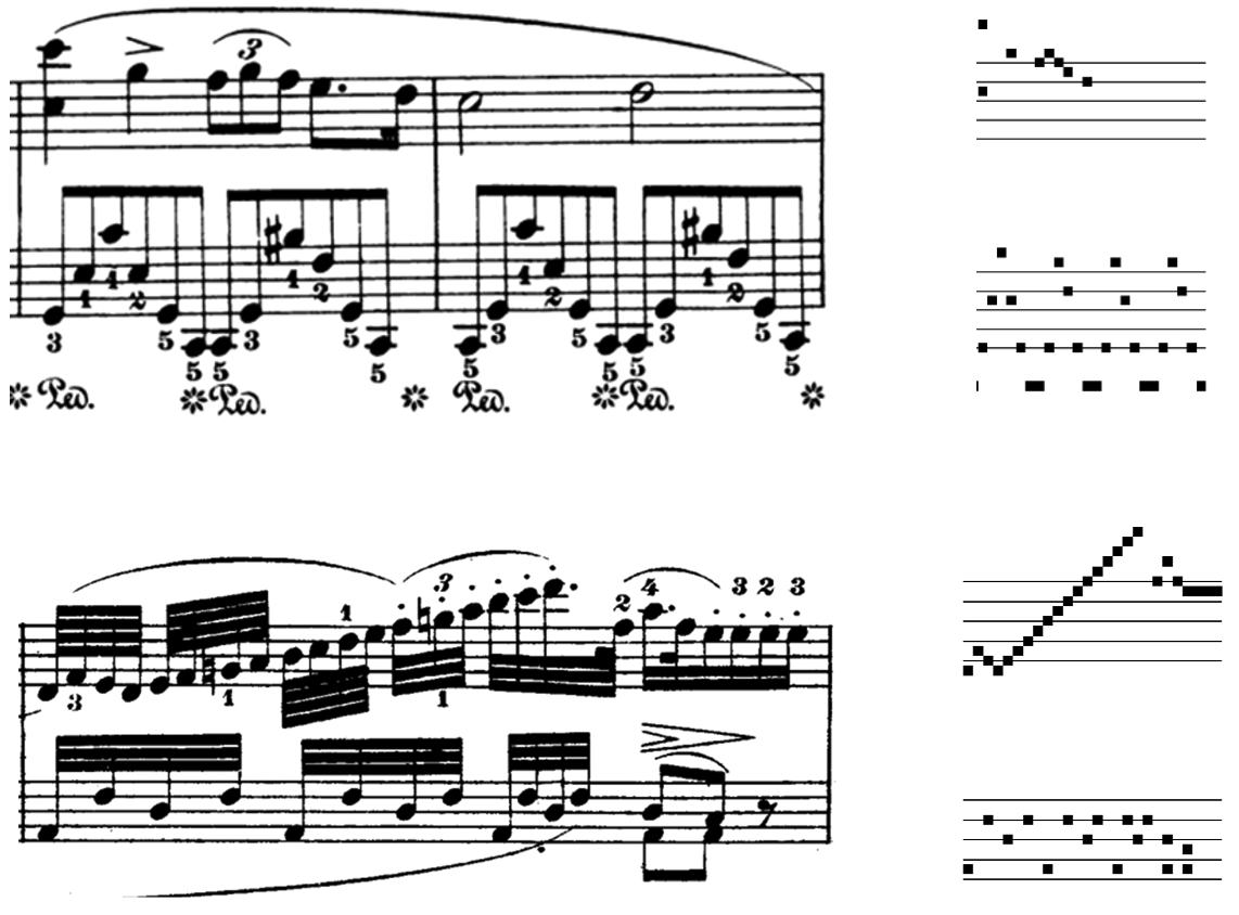
Figure 1: Two examples of a piano sheet music excerpt (left) and corresponding bootleg score representation (right).

It is worth mentioning a few practical details at this point. First, each 62-bit bootleg score column is encoded as a single 64-bit integer, so that bootleg scores are compactly represented as a list of integers. As a result, each sheet music PDF is reduced to a list of lists of 64-bit integers, where the first list corresponds to different pages and the second list corresponds to different bootleg score events on a page. This representation makes it possible to store an inconveniently large ($>10$TB in PNG format) dataset very compactly in memory. Second, the resulting repository after the fourth step above is the IMSLP piano bootleg scores data v1.0, which was originally presented in Yang and Tsai (2020). The fifth step (below) describes the improvements in the newly released v1.1 dataset, in which bootleg scores arising from non-music pages have been identified and removed.

The fifth step is to filter out non-music pages from the bootleg score repository. One of the problems with the original repository is that many PNG images are not sheet music – they may be title pages, blank pages, foreword, table of contents, etc. In the original v1.0 repository, a bootleg score was computed on every single PNG image, without any consideration of the contents in the image. This results in a non-trivial amount of gibberish bootleg score data which has been extracted from non-music images. In order to identify non-music pages, we trained a Transformer-based model to identify gibberish bootleg scores. The process for training this model is described in detail in the next subsection. In the revised v1.1 IMSLP piano bootleg scores repository, the bootleg scores for (predicted) non-music pages have been identified and removed.

3.2 Identifying Non-music Pages

In this subsection, we describe the process of identifying non-music pages by training a Transformer-based model on bootleg score fragments.

The first step is to label a set of music and non-music pages. This was done in the following manner. First, we took the original 9-way dataset proposed in Tsai and Ji (2020), in which each page had been manually labeled as music or non-music. We manually re-labeled these pages into three categories: music, non-music, or mixture. The “mixture” category contains pages that contain both sheet music and text, as is often seen in a table of contents (e.g. showing excerpts of pieces) or foreword. We ultimately decided to exclude the mixture pages from training, and only include pure music and pure non-music pages for training our classifier. In total, there were 5938 music pages and 259 non-music pages. We divided these pages into training and validation partitions using a 60-40 split.

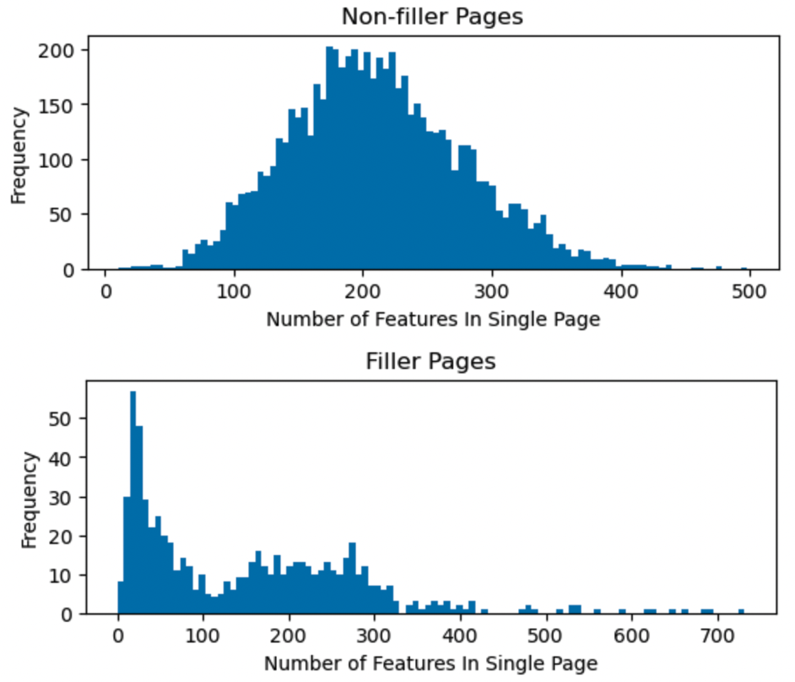
(a)

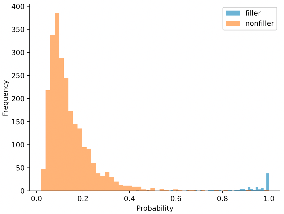
(b)

Figure 2: (a) Histogram of the number of bootleg score features in a set of manually labeled music pages (top) and non-music pages (bottom). (b) Predicted probability of an ensembled classifier that classifies validation pages as filler (non-music) vs non-filler. We use a hard threshold of 0.5 to ensure that filler pages are excluded from our dataset with high confidence.

The second step is to sample bootleg score fragments. Figure 2(a) shows a histogram of the number of bootleg score features in music pages (upper pane) and non-music pages (lower pane). We can see that many filler (non-music) pages have a very small number of bootleg score features, so our classifier will need to handle short bootleg score fragments. Accordingly, we decided to train our model on bootleg score fragments of length 16. We densely sampled bootleg score fragments from the non-music pages by sampling 16-length fragments with 50% overlap. This resulted in a total of 2799 non-music bootleg score fragments (1689 train, 1110 validation). To maintain a balanced dataset, we randomly sampled the same number of fragments from the music pages. This sampling was done by randomly sampling a piece (PDF) from the train/validation partition, randomly sampling a music page from the PDF, and then randomly sampling a length 16 fragment from the page’s bootleg score. At the end of this step, we have a labeled dataset of 3378 training bootleg score fragments (1689 filler, 1689 non-filler) and 2220 validation bootleg score fragments (1110 filler, 1110 non-filler).

The third step is to train a music vs non-music fragment classifier. We adopted a similar approach as in Tsai and Ji (2020), which we describe here for completeness. We encode each 62-bit bootleg score column as a sequence of eight 8-bit characters, and learn a subword vocabulary using Byte Pair Encoding (Gage, 1994). Using this BPE tokenizer, we pretrain a GPT-2 language model on the entirety of the IMSLP piano bootleg scores repository (v1.0). Next, we add a classification head with two output classes (music vs non-music) and finetune it on the labeled dataset of music and non-music fragments. In this way, our classifier is trained to classify 16-length bootleg score fragments as music or non-music.

We apply our classifier model to full pages in the following manner. We first extract a bootleg score representation from the page. If the resulting bootleg score has a length less than 64, it is automatically classified as non-music. (Note from Figure 2(a) that very few music pages have bootleg score lengths less than 64.) Otherwise, fragments of length 16 are densely sampled from the bootleg score with 50% overlap, and each fragment is passed through our classifier model. We average the outputs of each fragment prediction to get an ensembled prediction for the entire page.

Figure 2(b) shows a histogram of predicted probabilities on the validation pages, where a higher probability corresponds to a non-music page. We can see that there is a fairly clean separation between the music and non-music data. We set a very conservative threshold of 0.5, which ensures that non-music pages will be excluded from the data with high confidence (and sometimes music data will be excluded as well, which we are okay with). With this threshold value, we achieve a precision of 0.85 and a recall of 0.98 on the validation pages. Because we care more about ensuring that non-music pages are excluded, the recall of 0.98 is the more important metric. We use this ensembled classifier to identify and remove non-music pages from the IMSLP piano bootleg score repository.

4 Dataset Preparation: Labeled Data

In this section, we describe the preparation of the labeled (100-way, 9-way) PBSCSR data. The 9-way and 100-way data provide labeled bootleg score fragments to train and evaluate models for the composer style recognition task at varying levels of difficulty.

The first step is to identify a list of 100 composers to include. We first ranked all composers by the total amount of bootleg score data they have available on IMSLP. We then manually reviewed the ordered list of composers and selected the top 100, being sure to remove those who are not primarily composers (e.g. some people on the list were primarily arrangers and editors). For the 9-way dataset, we adopted the same list of composers as in Tsai and Ji (2020): Bach, Beethoven, Chopin, Haydn, Liszt, Mozart, Schubert, Schumann, and Scriabin.

The second step is to select a set of sheet music PDFs for each composer. Each piece in IMSLP may have multiple PDFs associated with it, which correspond to different publishers or editions. Because popular pieces tend to have a large number of sheet music versions, we select one representative PDF per piece in order to avoid over-representing a small number of pieces. In order to maximize the amount of data available to us, we simply selected the PDF that had the highest number of total bootleg score events. Figure 3(a) shows the total number of pieces available for these top 100 composers, and Figure 3(b) shows the total number of bootleg score events per composer.

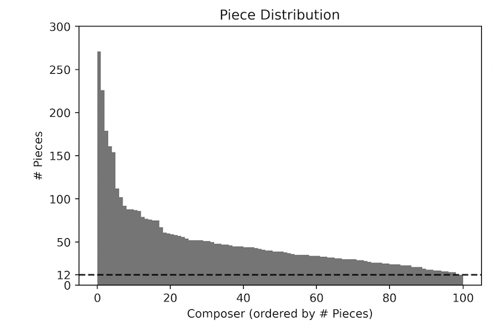
(a)

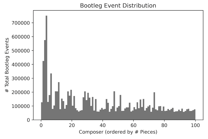
(b)

Figure 3: (a) The total number of pieces available on IMSLP for the composers in the 100-way dataset. (b) The total number of bootleg score events for each composer in the 100-way dataset.

The third step is to identify non-music pages in the selected set of PDFs. We used a Transformer-based model to identify filler pages, as described in Section 3.2. Table 2 shows the number of pieces, total number of pages, number of (predicted) non-music pages, and number of bootleg score events for each composer in the 9-way labeled dataset. There are 896 PDFs, 10305 pages with music content, and $2.2$ million bootleg score features. In the 100-way labeled dataset, there are 4997 PDFs, 64129 pages with music content, and $12.1$ million bootleg score features.

Composer	# Pieces	# Pages	# Bootleg
		(all/music)	Features
Bach	226	1752/1666	424948
Beethoven	86	1292/1170	272374
Chopin	89	1048/996	205513
Haydn	51	50/50	12408
Liszt	179	3405/3170	575367
Mozart	61	702/673	174355
Schubert	88	836/836	206103
Schumann	40	981/919	206379
Scriabin	76	879/825	135851
9-way	896	10945/10305	2213298
100-way	4997	70440/64129	12108749

Table 2: Overview of the raw sheet music data from which the 9-way PBSCSR data was constructed. Cumulative counts for the 100-way data are also shown at the bottom.

The fourth step is to sample bootleg score fragments from each composer. This is done in the following manner. First, we divide the pieces into training, validation, and test sets, using a split of 70%, 15%, and 15%, respectively. Splitting at the piece level ensures that there will be no data leakage between train and test fragments. Next, we decided on the total number of bootleg score fragments to sample from each partition. For the 9-way data, we have 28000 train fragments, 6000 validation fragments, and 6000 test fragments, resulting in a total of 40000 examples. For the 100-way data, we have 70000 train fragments, 15000 validation fragments, and 15000 test fragments, resulting in a total of 100,000 examples. Based on these numbers, we calculated how many fragments per composer need to be sampled in order to achieve class balance. Each fragment is drawn by randomly selecting a piece by a given composer, and then randomly selecting a 64-length fragment from the bootleg score. Our sampling process guarantees that our classes are perfectly balanced, and it gives equal weight to all pieces (in IMSLP) that a composer has composed.

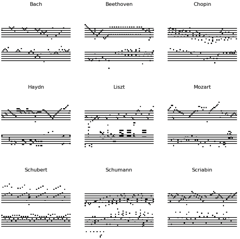
Figure 4: Example bootleg score images from the labeled 9-way PBSCSR data. Staff lines have been overlaid for reference.

Figure 4 shows a set of example bootleg score images from the 9-way dataset. For ease of reference, the staff lines in the left and right hands have been overlaid. Even without any information about note durations, key or time signature, or accidentals, one can immediately see some recognizable features: the Bach example has fugue-like texture and movement. The Beethoven example has an alternating octave in the right hand, which is not common in (say) Bach’s music. The Mozart example has scale-like runs in the right hand with an Alberti bass-like left hand accompaniment. The Classical and Baroque composers (Bach, Mozart, Haydn) have thinner textures compared to the Romantic era composers. These examples show that, even with the noisy bootleg score representation, many aspects of compositional style are preserved.

The 9-way and 100-way labeled datasets are formatted in a way that mimics the MNIST dataset. Each dataset consists of the following six arrays:

• $X_{train}$: a $N_{train}\times 62\times 64$ binary tensor specifying the training bootleg score fragments, where $N_{train,9way}=28000$ and $N_{train,100way}=70000$

• $Y_{train}$: a $N_{train}$ length array specifying the train composer class indices

• $X_{valid}$: a $N_{valid}\times 62\times 64$ binary tensor specifying the validation bootleg score fragments, where $N_{valid,9way}=6000$ and $N_{valid,100way}=15000$

• $Y_{valid}$: a $N_{valid}$ length array specifying the validation composer class indices

• $X_{test}$: a $N_{test}\times 62\times 64$ binary tensor specifying the test bootleg score fragments, where $N_{test,9way}=6000$ and $N_{test,100way}=15000$

• $Y_{test}$: a $N_{test}$ length array specifying the test composer class indices

In addition, we also provide relevant metadata on all train, validation, and test fragments. This metadata includes a unique identifier that specifies the PDF from IMSLP from which the fragment was taken, as well as the page and offset in the bootleg score from which the fragment was sampled. This information is valuable to researchers who wish to go back to the raw sheet music image data, perhaps for debugging, visualization, and deeper understanding.

The 100-way dataset poses a much more challenging task than the 9-way dataset. One may notice that the shape and size of the data is similar to MNIST, in keeping with our motto of constructing a dataset that is “as accessible as MNIST and as challenging as ImageNet.” Each composer only has 700 training examples, so the task is difficult both for the large number of composers and the relative scarcity of labeled data. For these reasons, we believe this dataset will push the boundaries of composer style recognition to the next level.

5 Research Tasks

In this section, we describe several research tasks that could be studied with the PBSCSR dataset. We also provide baseline results using standard techniques for future researchers to compare against.

5.1 Model-based composer style recognition

The most obvious task is a model-based composer style recognition task. Here, the goal is to classify a bootleg score fragment according to its composer class. In addition to a set of ($x_{i}$, $y_{i}$) training pairs, a large set of unlabeled variable-length piano bootleg scores from IMSLP is also available for pretraining models.

There are several metrics of performance that might be appropriate in this scenario. Following the convention in ImageNet, one useful metric of performance is top $N$ accuracy, which indicates the percentage of queries that have the correct composer in the $N$ highest-ranked composers. Another useful metric is mean reciprocal rank, which is calculated as

$$MRR=\frac{1}{N}\sum_{i=0}^{N-1}\frac{1}{R_{i}}$$ (1)

where $R_{i}$ indicates the rank of the true composer. We recommend reporting results with several of the above metrics, since the most appropriate metric may depend on the difficulty of the task.

Tables 3 and 4 show the performance of three different baseline systems on the 9-way and 100-way classification tasks, respectively. The first baseline system is a CNN model with two convolutional layers, followed by global average pooling across time, and then a final output linear classification layer. This model is based on the architecture proposed in (Verma and Thickstun, 2019) but adapted to a bootleg score representation (instead of MIDI). The second baseline system is a GPT-2 model (Radford et al., 2019) trained in the same manner as in Section 3.2: each bootleg score column is represented as a sequence of 8-bit characters, a subword vocabulary is learned using Byte Pair Encoding, a small 6-layer GPT-2 language model is trained on unlabeled bootleg scores in IMSLP, and the model is fine-tuned on the labeled data. To tease apart the effect of pretraining and finetuning, we report results of the GPT-2 model under three different training conditions: (1) training the model from scratch on the labeled data without pretraining (“GPT-2 (no pretrain)”), (2) pretraining the language model and learning a linear probe (“GPT-2 (LP)”), and (3) pretraining the language model, learning a linear probe, and then unfreezing and finetuning the whole model (“GPT-2 (LP-FT)”). For (3), we followed the recommended practices in Kumar et al. (2022), which were shown to have good generalization to out-of-distribution data. The third baseline system is a RoBERTa model (Liu et al., 2019) with 6 Transformer encoder layers. This model is pretrained using a masked language modeling task, but otherwise trained in a similar manner as GPT-2. We report results of the RoBERTa model under the same three training conditions as above. These three model architectures were previously explored in Tsai and Ji (2020) and Yang and Tsai (2021a) on a 9-way composer classification task, and here we present results on the (new) 9-way and 100-way PBSCSR tasks. These results are intended to serve as baselines which future approaches can compare against.

System	Top 1	MRR
CNN	40.0	0.593
GPT-2 (LP-FT)	49.6	0.670
GPT-2 (LP)	42.5	0.613
GPT-2 (no pretrain)	25.0	0.466
RoBERTa (LP-FT)	44.4	0.631
RoBERTa (LP)	38.0	0.581
RoBERTa (no pretrain)	19.2	0.407

Table 3: Baseline results for the 9-way PBSCSR task. Results are shown for top 1 accuracy (%) and mean reciprocal rank.

There are two things to notice about the baseline results in Tables 3 and 4. First, the GPT-2 model has the best performance among the three models on both the 9-way and 100-way tasks. We can see that pretraining on the unlabeled IMSLP data makes a big difference, improving top-1 accuracy on the 9-way task from 25.0% to 42.5% and improving top-5 accuracy on the 100-way task from 11.6% to 28.5%. This underscores the importance of having a large, diverse set of data for pretraining. We also see that full model fine-tuning makes a big difference, improving top-1 accuracy on the 9-way task from 42.5% to 49.6% and improving top-5 accuracy on the 100-way task from 28.5% to 34.8%. Second, there is a lot of room for improvement. The best GPT-2 model only achieves a top-5 accuracy of 34.8% on the 100-way task, showing that there is a massive amount of room for improvement. Our hope is that this dataset can spur progress on this challenging task.

System	Top 1	Top 5	Top 10
CNN	7.4	21.3	32.4
GPT-2 (LP-FT)	13.9	34.8	49.0
GPT-2 (LP)	10.4	28.5	42.8
GPT-2 (no pretrain)	3.2	11.6	20.4
RoBERTa (LP-FT)	10.6	29.0	42.0
RoBERTa (LP)	7.5	22.9	35.0
RoBERTa (no pretrain)	2.1	8.1	15.0

Table 4: Baseline results for the 100-way PBSCSR task. Results are shown for top 1, top 5, and top 10 accuracy (%).

5.2 Few-shot composer style recognition

An interesting modification to the above problems is to study few-shot composer style recognition. The problem setup would be the same as before, but the number of training examples per composer would be artificially limited to $N$. We recommend the following tasks: (a) a 9-way classification task with $N=1$, $10$, $100$ and (b) a 100-way classification task with $N=1$, $10$, $100$. This set of tasks encourages the development of approaches that are data-efficient (with labeled data), and it allows one to study the effect of the number of training examples as well as the generalizability of model representations.

System	N	Top 1	Top 1	MRR	MRR
		mean	std	mean	std
GPT-2	1	15.4	2.3	0.36	.020
RoBERTa	1	14.5	1.8	0.35	.017
Random	1	11.2	0.3	0.32	.003
GPT-2	10	19.7	1.8	.407	.013
RoBERTa	10	19.8	1.6	.406	.013
Random	10	11.0	0.4	.314	.003
GPT-2	100	23.8	0.8	.449	.006
RoBERTa	100	23.7	0.9	.446	.006
Random	100	11.1	0.4	.314	.004

Table 5: Baseline results for the $N$-shot 9-way classification task. Results are expressed as a mean and standard deviation across 30 trials. Top 1 accuracies are indicated in percentages (%).

System	N	Top 1	Top 1	Top 5	Top 5	Top 10	Top 10
		mean	std	mean	std	mean	std
GPT-2	1	1.9	.21	7.7	.44	14.1	.56
RoBERTa	1	1.8	.20	7.7	.45	14.1	.57
Random	1	1.0	.06	5.0	.13	10.0	.21
GPT-2	10	3.0	.25	11.2	.38	19.1	.50
RoBERTa	10	3.1	.19	11.3	.39	19.3	.54
Random	10	1.0	.10	5.0	.15	10.0	.23
GPT-2	100	3.9	.17	14.2	.30	23.5	.41
RoBERTa	100	4.0	.14	14.3	.27	23.7	.34
Random	100	1.0	.07	5.0	.16	10.0	.21

Table 6: Baseline results for the few-shot 100-way classification task. Results are expressed as a mean and standard deviation of test set accuracy (%) across 30 trials.

We consider three baseline models for the few-shot tasks. The first system is a GPT-2 model that is trained by: (a) pretraining a 6-layer GPT-2 language model on the unlabeled IMSLP bootleg score data, as described in Section 5.1, (b) using the penultimate activations of the language model as a feature representation for the training samples, (c) identifying the $k$ nearest neighbors for each composer that are closest in euclidean distance to a given test query, and (d) rank ordering the composers by average euclidean $k$ nearest neighbor distance. The second system is a 6-layer RoBERTa model that is trained and used in a similar manner, but using a masked language modeling task during pretraining. These models adopt the pretraining strategies of the classification models described in Section 5.1, but use $k$ nearest neighbors for classification instead of training a classification layer. We also evaluate the performance of a random guessing baseline for reference.

Tables 5 and 6 show the performance of the three baseline systems on the few-shot 9-way and 100-way tasks, respectively. The upper, middle, and bottom sections of the table show performance for an $N$-shot task with $N=1$, $N=10$, and $N=100$, respectively. For $N=1$ we use the $k=1$ nearest neighbor for each composer (by necessity), and for $N=10$ and $N=100$ we use the $k=3$ nearest neighbors. In each trial, we randomly sample $N$ training examples from each composer to simulate a few-shot scenario, and then calculate the performance on the entire test set. We report the mean and standard deviation of performance across 30 trials.

We can see that the pretrained models perform significantly better than random, and that both models perform comparably across all settings. While these results show that the pretrained models are indeed extracting style information, the performance of these models is quite poor overall, indicating how much room there is for improvement. We provide these results as a baseline against which future works can compare.

5.3 0-shot composer style recognition

Another interesting problem to consider is zero-shot composer style recognition. In this task, the goal is to predict the composer of a bootleg score fragment when no previous training examples of that composer have been seen. We are not aware of previous work studying this topic within the composer style recognition literature until very recently, where researchers explore zero-shot composer classification with music-text data (Wu et al., 2023). Here, we simply define the task and suggest some possible avenues of exploration.

This task is possible due to the rich metadata available on IMSLP. For example, given the Wikipedia articles for some unknown composers, one could infer aspects of compositional style based on their date of birth, country of origin, connections to other composers, or other knowledge about the composer that is embedded in a large language model. Wu et al. (2023) train a model to embed both symbolic music and text descriptions into a common embedding space using a CLIP-like approach (Radford et al., 2021). This work does not release their music-text training pairs, however, and also evaluates on a small evaluation dataset (411 pieces, 8 classes). The PBSCSR data would be sufficiently large to train such models, is open to the research community, and offers a much more challenging classification task. Setting up a benchmark for multimodal tasks such as this is an area for future work.

The zero-shot task opens the door to multimodal approaches to composer style recognition. Given the size, richness of metadata, and open nature of IMSLP, we believe that the PBSCSR data is well poised to facilitate interesting and novel directions in multimodal research.

6 Research Questions

In this section, we describe several research questions that we believe the PBSCSR data is especially well suited to facilitate research on.

6.1 Encoding Schemes

One open research question is, “How should we encode music data when feeding it into a model?" We may want to select the encoding scheme to maximize performance on a particular task of interest, to have certain desirable properties such as key or tempo invariance, or some combination of factors. Because of our design decision to use a bootleg score representation, the PBSCSR data has discarded a significant amount of musical information. Nonetheless, due to its simple format, it is well poised to facilitate rapid, iterative exploration of many interesting questions, some of which we describe below.

Image vs Tokens. The fact that the bootleg score is a binary matrix raises the question: Is it better to treat the data as a 2D binary image or as a sequence of discrete tokens (e.g. each bootleg score column is interpreted as a discrete “word")? These two options lead to different kinds of models: 2D images lend themselves to CNN or ViT-based architectures, while token sequences lend themselves to Transformer-based language models. Previous work (Yang and Tsai, 2021a) has compared simple CNN architectures with GPT-2 and RoBERTa, but a lot of recent work has developed effective strategies for applying Transformers to images (e.g. ViT (Dosovitskiy et al., 2021)) and utilizing pretraining strategies like masked autoencoding (e.g. ViT-MAE (He et al., 2022)). It is unclear which representation is more effective, or what advantages and disadvantages each representation brings.

Harmonic vs Temporal. What are effective ways to capture both harmonic and temporal information? The approach described in Section 5.1 encodes bootleg score columns (or parts thereof) as discrete tokens, and then models temporal information with a Transformer. But one could alternately encode rectangular blocks of the bootleg score image as discrete tokens, similar to the patches in a ViT model. In this case, each token would capture both harmonic and temporal information, rather than only harmonic information.

Raw vs Processed. At what level of semantic representation is it best to represent discrete tokens? On one end of the spectrum, we could represent a bootleg score fragment simply as a sequence of zeros and ones, and then let a Byte Pair Encoder combined with a Transformer model learn the most suitable representation. On the other end of the spectrum, we could design musically-informed encodings, taking into account domain knowledge such as the split between the left and right hand staves, the fact that staff line positions are cyclical and octave-based, etc. For example, one could encode a bootleg score column as the text “C3-G3-E4-C5", which explicitly decomposes the staff line position into octave and class information.

Absolute vs Relative. How much should the encoding of discrete tokens capture absolute vs relative position information? One intuitive shortcoming of the Transformer models in Section 5.1 is that they encode the absolute staff line positions of noteheads, rather than relative position or movement. In the example given above, the bootleg score column encoded as “C3-G3-E4-C5” could instead be encoded as “C3-4-5-5" to capture the relative staff line intervals between notes in the chord. Furthermore, the root of the chord (C3) could itself be expressed relative to a notehead in a previous bootleg score column.

The topics above are issues that could be studied conveniently with the PBSCSR data. Many other similar questions could be rapidly explored, given the simplicity and format of the data. Thus, even though the dataset does not have complete symbolic score information, it can facilitate rapid exploration of ideas and progress on research questions of broad interest to the MIR community.

6.2 Data Augmentation

Another open research question is, “What are effective ways to perform data augmentation of symbolic music data?" The PBSCSR data is ideal for exploring data augmentation techniques for two reasons, which we describe below.

First, the PBSCSR data has a very simple format. The fact that the bootleg score is a simple 2D image makes it much easier to explore data augmentation techniques. For example, many data augmentation strategies developed for computer vision can be applied out-of-the-box with no additional effort, such as cropping, shifting, and MixUp (Zhang et al., 2018). In contrast, for symbolic music formats like MusicXML, it would be much more cumbersome to rapidly explore the same types of data augmentation. Both existing and novel techniques would be far easier to implement with bootleg score images than with MusicXML data.

Second, the PBSCSR data format has several key properties that make such augmentations musically meaningful. One such property of the bootleg score is the nature of key changes: because the staff line positions (A through G) are cyclical, key changes correspond to simple vertical shifts in the bootleg score representation. Similarly, shifts in time correspond to simple horizontal shifts in the bootleg score representation. The bootleg score also has the property of additivity – if you add a bootleg score event describing a chord in the right hand to a bootleg score event describing a left hand chord, the resulting event is simply the sum of the two constituent bootleg scores. (Note that discrete token-based representations do not have this property.) It is also worth pointing out that the bootleg score representation is inherently invariant to tempo, since it only captures the sequence of noteheads rather than describing the absolute time between note events. Because of these properties, operations like cropping and shift and MixUp are very easy to implement and have clear musical interpretations.

The above properties make the PBSCSR dataset ideal for exploring data augmentation strategies. This includes exploring the effectiveness of existing data augmentation techniques from computer vision, as well as quickly implementing and trying domain-specific data augmentation techniques.

6.3 Integrating Multimodal Information

Yet another interesting research question is, “How can we train models with multiple modalities of data?" This is a very active area of interest in the machine learning community, with influential models like CLIP (Radford et al., 2021) and Stable Diffusion (Rombach et al., 2022) gaining a lot of public attention. The PBSCSR dataset is ideal for exploring this question in MIR for three reasons, which we describe below.

First, the PBSCSR data is linked to rich metadata on IMSLP. In particular, each piece in IMSLP has a lot of rich multimodal information: audio recordings, MIDI files, sheet music scores, arrangements and transcriptions, relevant metadata (e.g. composer, publisher information, composition date, composer time period, instrumentation), and links to relevant Wikipedia article pages and descriptions (e.g. All Music Guide). Importantly, in keeping with IMSLP’s philosophy, these resources generally have very research-friendly licenses – most audio recordings and sheet music scores have a Creative Commons license or are in the public domain.

Second, the PBSCSR dataset is large enough to study multimodal problems at a nontrivial scale. Given the size and scale of modern models, it is necessary to have a large enough quantity of data to train large models. The PBSCSR dataset – and certainly IMSLP – fulfills this requirement. One additional benefit of utilizing IMSLP data is that the website is actively maintained, so the quantity of data will presumably only increase into the future.

Third, the bootleg score representation is well suited for cross-modal and multimodal tasks. Previous works have demonstrated the effectiveness of the bootleg score representation for cross-modal tasks. For example, it has been used in cross-modal retrieval to find matches between the Lakh MIDI Dataset and sheet music in IMSLP (Yang and Tsai, 2021b), and it has been used in cross-modal transfer learning to perform composer classification of audio recordings using sheet music as training data (Yang and Tsai, 2021a). As such, it is well suited to connect multiple representations of music, including sheet music images, symbolic files, and audio.

For these reasons, we believe the PBSCSR dataset is particularly well situated to facilitate multimodal research in MIR. Setting up the infrastructure for specific multimodal tasks is an area for future work.

7 Conclusion

This article motivates, describes, and presents the PBSCSR dataset for studying composer style recognition of piano sheet music. Our overarching goal was to create a dataset for studying composer style recognition that is “as accessible as MNIST and as challenging as ImageNet." To achieve this goal, we use a fixed-length bootleg score feature representation extracted from piano sheet music images on IMSLP. This choice allows us to access a large, open, diverse set of data while presenting the data in an extremely simple format that mimics MNIST images. The dataset itself contains labeled fixed-length bootleg score images for 9-way and 100-way classification tasks, as well as a large set of variable-length bootleg scores for pretraining. Additionally, we include metadata to indicate the specific piece, PDF score, and page from which each labeled training sample was taken, which can allow access to the raw sheet music images and other related metadata on IMSLP. We describe several research tasks that could be studied with the dataset and present baseline results for future works to compare against. We also discuss open research questions that the PBSCSR data is especially well suited to facilitate research on. For future work, we hope to extend the PBSCSR data with metadata on IMSLP to define benchmarks for multimodal tasks.

8 Acknowledgments

This material is based upon work supported by the National Science Foundation under Grant No. 2144050.

References

- Bogdanov et al. [2019a] Dmitry Bogdanov, Alastair Porter, Hendrik Schreiber, Julián Urbano, and Sergio Oramas. The acousticbrainz genre dataset: Multi-source, multi-level, multi-label, and large-scale. In Proceedings of the International Society for Music Information Retrieval Conference (ISMIR), pages 360–367, 2019a.
- Alajanki et al. [2016] Anna Alajanki, Yi-Hsuan Yang, and Mohammad Soleymani. Benchmarking music emotion recognition systems. PloS one, pages 835–838, 2016.
- Bogdanov et al. [2019b] Dmitry Bogdanov, Minz Won, Philip Tovstogan, Alastair Porter, and Xavier Serra. The MTG-jamendo dataset for automatic music tagging. In Proceedings of the International Conference on Machine Learning, 2019b.
- Wu and Yang [2023] Shih-Lun Wu and Yi-Hsuan Yang. Musemorphose: Full-song and fine-grained piano music style transfer with one transformer VAE. IEEE/ACM Transactions on Audio, Speech, and Language Processing, 31:1953–1967, 2023.
- Zhao et al. [2022] Yudong Zhao, György Fazekas, and Mark Sandler. Violinist identification using note-level timbre feature distributions. In Proceedings of the IEEE International Conference on Acoustics, Speech and Signal Processing (ICASSP), pages 601–605, 2022.
- Tzanetakis and Cook [2002] George Tzanetakis and Perry Cook. Musical genre classification of audio signals. IEEE Transactions on Speech and Audio Processing, 10(5):293–302, 2002.
- Yang et al. [2019] Daniel Yang, Thitaree Tanprasert, Teerapat Jenrungrot, Mengyi Shan, and TJ Tsai. MIDI passage retrieval using cell phone pictures of sheet music. In Proceedings of the International Society for Music Information Retrieval Conference (ISMIR), pages 916–923, 2019.