Online Algorithm for Node Feature Forecasting in Temporal Graphs

Abstract

In this paper, we propose an online algorithm mspace for forecasting node features in temporal graphs, which adeptly captures spatial cross-correlation among different nodes as well as the temporal autocorrelation within a node. The algorithm can be used for both probabilistic and deterministic multi-step forecasting, making it applicable for estimation and generation tasks. Comparative evaluations against various baselines, including graph neural network (GNN) based models and classical Kalman filters, demonstrate that mspace performs at par with the state-of-the-art and even surpasses them on some datasets. Importantly, mspace demonstrates consistent robustness across datasets with varying training sizes, a notable advantage over GNN-based methods requiring abundant training samples to learn the spatiotemporal trends in the data effectively. Therefore, employing mspace is advantageous in scenarios where the training sample availability is limited. Additionally, we establish theoretical bounds on multi-step forecasting error of mspace and show that it scales as ${\mathcal{O}}(q)$ for $q$-step forecast.

1 INTRODUCTION

Temporal graphs are a powerful tool for modelling real-world data that evolves over time. They are increasingly being used in diverse fields, such as recommendation systems, social networks, and transportation systems, to name a few. Temporal graph learning (TGL) can be viewed as the task of learning on a sequence of graphs that form a time series. The changes in the graph can be of several types: changes to the number of nodes, the features of existing nodes, the configuration of edges, or the features of existing edges. Moreover, a temporal graph can result from a single or a combination of these changes. The TGL methods can be applied to various tasks, such as regression, classification, and clustering, at three levels: node, edge, and graph (Longa et al., 2023).

In this work, we focus on node feature forecasting, also known as node regression, in which the previous temporal states of a graph are used to predict the future node features of that graph. In most neural network (NN) based models, the previous states are encoded to a super-state, which is then used to predict the future node features. This approach lacks interpretability, as the value of these super-states cannot be explained numerically, and the encoding function acts like a black box. Moreover, the success of NN-based methods relies on a training phase in which the model is learnt and later deployed. During this training phase, the model imparts meaning to the super-states. Leveraging the simplicity of Markov models, we intuitively define the state of a graph at a given time and propose a lightweight model capable of being deployed without any training. In other words, we propose an online algorithm for node feature forecasting that is well-suited for temporal graphs, given their dynamic nature. Such algorithms can be equipped with a mechanism to prioritise recent trends in the data over historical ones, thereby adapting to the changes in data distribution.

Adopting a Markovian approach, we establish a relation between the changes in node features, called shock, at the current step and the shock in the subsequent step. Despite the overly simplified Markov approximation, the conditional distribution can capture the complex spatio-temporal patterns within the graph data, as shown by the performance of our proposed model. Furthermore, we derive a theoretical upper bound on the prediction error of mspace, which scales linearly with the number of forecast steps. We also design a synthetic temporal graph generator, which allows us to derive data-centric insights from the model.

The rest of the paper is organised as follows. In Sec. 2, we present our algorithm in detail, and then compare it with relevant works in Sec. 3. We outline the different datasets and baselines that are used for evaluation in Sec. 4, and present the results for single-step and multi-step node feature forecasting in Sec. 5. Lastly, we conclude with some remarks in Section 6.

2 METHODOLOGY

2.1 Problem Setting

The temporal graph at time $t\in[T]$ can be represented as ${\mathcal{G}}_{t}=({\mathcal{V}},{\mathcal{E}},{\bm{X}}_{t})$, where ${\mathcal{V}}=[n]$ is the set of nodes, and ${\mathcal{E}}\subseteq{\mathcal{V}}\times{\mathcal{V}}$ is the set of edges. The node feature matrix is denoted as ${\bm{X}}_{t}=\begin{bmatrix}{\bm{x}}_{t}(v)\end{bmatrix}^{\top}_{v\in{\mathcal{V}}}\in\mathbb{R}^{n\times d}$ where ${\bm{x}}_{t}(v)\in\mathbb{R}^{d}$ is the feature vector of node $v\in{\mathcal{V}}$ at time $t$. The set of edges ${\mathcal{E}}$ can be represented by the adjacency matrix denoted as ${\bm{A}}\in\{0,1\}^{n\times n}$.

Forecasting problem: Predict the future feature matrices $\{{\bm{X}}_{t}:t\geq\tau\}$ given the past feature matrices $\{{\bm{X}}_{t}:t<\tau\}$, and adjacency matrix ${\bm{A}}$.

2.2 Markov Approximation

Instead of directly dealing with the node feature vector, we work with the difference between two time-adjacent feature vectors and refer to them as shocks. The shock at time $t$ for node $v\in{\mathcal{V}}$ is defined as

$$\bm{\varepsilon}_{t}(v)\triangleq\bm{x}_{t}(v)-\bm{x}_{t-1}(v).$$ (1)

In statistics, this is known as differencing (Shumway & Stoffer, 2017), whereby a non-stationary time series is expected to become stationary in the mean sense. Sometimes, differencing is performed repeatedly until the resultant time series is almost stationary.

We approximate the shocks as a Markov chain

$$p\left(\bm{\varepsilon}_{t+1}\mid\bm{\varepsilon}_{t},\bm{\varepsilon}_{t-1}.\cdots\right)\approx p\left(\bm{\varepsilon}_{t+1}\mid\bm{\varepsilon}_{t}\right),$$ (2)

and realise it through a pair of functions: $\Psi(\cdot)$, the state function, and $\Omega(\cdot)$, the sampling function. The state function returns the state from the current shock which is then fed to the sampling function to obtain the next shock.

$${\bm{s}}_{t}=\Psi(\bm{\varepsilon}_{t}),$$ (3)

$$\bm{\varepsilon}_{t+1}\approx\Omega({\bm{s}}_{t}).$$ (4)

The next shock can be estimated from the current shock as $\bm{\varepsilon}_{t+1}\approx\Omega\circ\Psi(\bm{\varepsilon}_{t})$ as illustrated in Fig. 1.

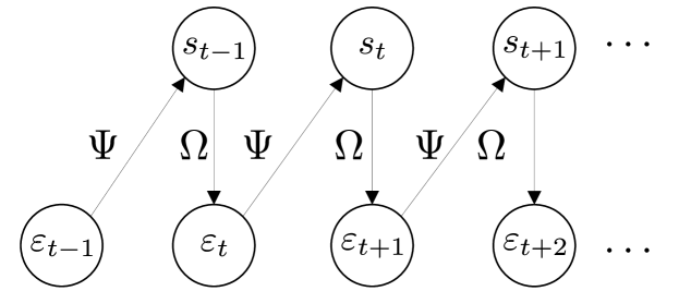
Figure 1: Approximating the shocks as a Markov chain.

Instead of learning the conditional distribution $p(\bm{\varepsilon}_{1+1}\mid\bm{\varepsilon}_{t})$, we learn $p(\bm{\varepsilon}_{1+1}\mid{\bm{s}}_{t})$, and estimate the next shock as

$$\bm{\varepsilon}_{t+1}\approx\Omega({\bm{s}}_{t})\sim p(\bm{\varepsilon}_{t+1}\mid{\bm{s}}_{t}).$$ (5)

2.3 Neighbourhood Sampling

We assume that the feature of node $v$ is impacted by the variations in the features of its neighbours. In the case of sparse graphs, we can also consider up to $K$-hop neighbours affecting a node’s feature vector. For graphs that are densely connected, we can sample a fixed number of neighbours from the set ${\mathcal{U}}_{v}$.

The set of nodes that are at most $K$-hops away from node $v$ are defined as $\displaystyle{\mathcal{U}}_{v}\triangleq\{u:\tilde{{\bm{A}}}_{v,u}=1,\forall u\in{\mathcal{V}}\}$, where $\tilde{{\bm{A}}}\triangleq\mathbb{I}\left\{\left({\bm{I}}+\sum_{k\in[K]}{\bm{A}}^{k}\right)\succ\mathbf{0}\right\}$.

To facilitate the explanation of our method, we introduce a notation ${\bm{x}}_{t}^{[{\mathcal{U}}]}$ which is the concatenation of ${\bm{x}}_{t}(u),\forall u\in{\mathcal{U}}$. Similarly, $\bm{\varepsilon}_{t}^{[{\mathcal{U}}]}={\bm{x}}_{t}^{[{\mathcal{U}}]}-{\bm{x}}_{t-1}^{[{\mathcal{U}}]}$.

2.4 State Function

We introduce two variants of the state function:

• $\Psi:\mathbb{R}^{|{\mathcal{U}}_{v}|d}\rightarrow\{0,1\}^{|{\mathcal{U}}_{v}|d}$ with $\Psi(\bm{\varepsilon}_{t})\triangleq\mathbb{I}\{\bm{\varepsilon}_{t}\succ\bm{0}\}$ which returns a binary vector corresponding to the spatial patterns in the data.

• $\Psi:\mathbb{N}\rightarrow[\tau_{0}]$ with $\Psi(t)\triangleq t\,{\rm mod}\,\tau_{0}$ captures the temporal patterns in the data, where $\tau_{0}$ is the seasonal time period, i.e., repeated intervals within which the data has similar behaviour.

2.5 Sampling Function

In equation 5 we defined the sampling function as a sample from the conditional distribution, which is probabilistic and yields a variable output. Additionally, we define a deterministic sampling function which returns the mean instead of the sample. Thus, the two sampling functions are:

• $\Omega({\bm{s}}_{t})\sim p(\bm{\varepsilon}_{t+1}\mid{\bm{s}}_{t})={\mathcal{N}}(\bm{\varepsilon}_{t+1};\bm{\mu}({\bm{s}}_{t}),\bm{\Sigma}({\bm{s}}_{t}))$ is the probabilistic sampling function.

• $\Omega({\bm{s}}_{t})=\mathbb{E}[\bm{\varepsilon}_{t+1}\mid{\bm{s}}_{t}]=\bm{\mu}({\bm{s}}_{t})$ is deterministic although it changes as the learnt distribution evolves.

2.6 Algorithm

We name our algorithm mspace with a suffix specifying the state and sampling functions. For example, mspace-S${\mathcal{N}}$ represents the algorithm with spatial state function S, and probabilistic sampling function ${\mathcal{N}}$. In mspace-S*, for each node $v\in{\mathcal{V}}$, we approximate $p\left(\bm{\varepsilon}_{t+1}^{[{\mathcal{U}}_{v}]}\mid\Psi(\bm{\varepsilon}_{t}^{[{\mathcal{U}}_{v}]})\right)$ as a Gaussian distribution and learn its parameters through maximum likelihood estimation (MLE). Likewise, in mspace-T*, the distribution that is learnt for each node is $p(\bm{\varepsilon}_{t+1}(v)\mid\Psi(t))$. To estimate the distribution, we collect the samples corresponding to a given state in a queue of fixed size $M$. We denote a queue for node $v$ which collects samples for state ${\bm{s}}$ as ${\mathcal{Q}}_{v}({\bm{s}})$. The MLE solution is calculated as $\bm{\mu}_{v}({\bm{s}})={\rm mean}({\mathcal{Q}}_{v}({\bm{s}}))$, and $\bm{\Sigma}_{v}({\bm{s}})={\rm covariance}({\mathcal{Q}}_{v}({\bm{s}}))$. The use of a fixed-size queue ensures that the distribution prioritises recent data over historical data, thereby allowing the system to adapt to prevailing trends.

The shock prediction for node $v\in{\mathcal{V}}$ at time $t+q$ after having seen the shock at time $t$ is $\hat{\bm{\varepsilon}}_{t+q}(v)=(\Omega\circ\Psi)^{q}\left(\bm{\varepsilon}_{t}\right)$, and the node feature estimate at time $t+q$ is

$$\hat{{\bm{x}}}_{t+q}(v)={\bm{x}}_{t}(v)+\sum_{k\in[q]}\hat{\bm{\varepsilon}}_{t+k}(v).$$ (6)

We explain the working of mspace-S${\mathcal{N}}$ in Algorithm 1. For mspace-*$\mu$, $\hat{\bm{\varepsilon}}_{t}^{[{\mathcal{U}}_{v}]}\leftarrow\bm{\mu}_{v}({\bm{s}}^{*})$ replaces the sampling in steps 15 and 18, and $\bm{\Sigma}_{v}({\bm{s}})$ becomes redundant. The computational complexity of the different flavours of mspace is calculated in Appendix A.

Algorithm 1 mspace-S${\mathcal{N}}$

0:  ${\mathcal{G}}=({\mathcal{V}},{\mathcal{E}},{\bm{X}})$, $r\in[0,1)$, $q,M,K,\tau_{0}\in\mathbb{N}$

0:  $\hat{\bm{\varepsilon}}_{t}(v),\quad\forall v\in{\mathcal{V}},t\in[\lfloor r\cdot T\rfloor,T]$

1:  $\bm{\varepsilon}_{t}(v)\leftarrow{\bm{x}}_{t}(v)-{\bm{x}}_{t-1}(v),\quad\forall v\in{\mathcal{V}},\,t\in[T]$ Offline training:

2:  for $t\in[\lfloor r\cdot T\rfloor]$ do

3:     for $v\in{\mathcal{V}}$ do

4:        $\displaystyle{\bm{s}}_{t}^{[{\mathcal{U}}_{v}]}\leftarrow\Psi\left(\bm{\varepsilon}_{t}^{[{\mathcal{U}}_{v}]}\right)$

5:        ${\mathcal{S}}_{v}\leftarrow{\mathcal{S}}_{v}\cup\left\{{\bm{s}}_{t}^{[{\mathcal{U}}_{v}]}\right\}$

6:        ${\mathcal{Q}}_{v}\left({\bm{s}}_{t}^{[{\mathcal{U}}_{v}]}\right)\leftarrow$ append $\bm{\varepsilon}_{t+1}^{[{\mathcal{U}}_{v}]}$

7:     end for

8:  end for

9:  $\bm{\mu}_{v}({\bm{s}})\leftarrow{\rm mean}({\mathcal{Q}}_{v}({\bm{s}})),\quad\forall s\in{\mathcal{S}}_{v},v\in{\mathcal{V}}$

10:  $\bm{\Sigma}_{v}({\bm{s}})\leftarrow{\rm covariance}({\mathcal{Q}}_{v}({\bm{s}})),\quad\forall s\in{\mathcal{S}}_{v},v\in{\mathcal{V}}$ Online learning:

11:  for $t\in[\lfloor r\cdot T\rfloor,T-q]$ do

12:     for $v\in{\mathcal{V}}$ do

13:        $\displaystyle{\bm{s}}_{t}^{[{\mathcal{U}}_{v}]}\leftarrow\Psi\left(\bm{\varepsilon}_{t}^{[{\mathcal{U}}_{v}]}\right)$

14:        $\displaystyle{\bm{s}}^{*}\leftarrow\arg\min_{{\bm{s}}\in{\mathcal{S}}_{v}}\left\lVert{\bm{s}}-{\bm{s}}_{t}^{[{\mathcal{U}}_{v}]}\right\rVert$

15:        $\hat{\bm{\varepsilon}}_{t+1}^{[{\mathcal{U}}_{v}]}\sim{\mathcal{N}}(\bm{\varepsilon};\bm{\mu}_{v}({\bm{s}}^{*}),\bm{\Sigma}_{v}({\bm{s}}^{*}))$

16:        for $k\in[2,q]$ do

17:           $\displaystyle{\bm{s}}^{*}\leftarrow\arg\min_{{\bm{s}}\in{\mathcal{S}}_{v}}\left\lVert{\bm{s}}-\Psi\left(\hat{\bm{\varepsilon}}_{t+k-1}^{[{\mathcal{U}}_{v}]}\right)\right\rVert$

18:           $\hat{\bm{\varepsilon}}_{t+k}^{[{\mathcal{U}}_{v}]}\sim{\mathcal{N}}(\bm{\varepsilon};\bm{\mu}_{v}({\bm{s}}^{*}),\bm{\Sigma}_{v}({\bm{s}}^{*}))$

19:        end for

20:        $\hat{\bm{\varepsilon}}_{t+k}(v)\leftarrow\hat{\bm{\varepsilon}}_{t+k}^{[{\mathcal{U}}_{v}]}(v),\quad\forall k\in[q]$

21:        Update ${\mathcal{S}}_{v},{\mathcal{Q}}_{v}$

22:        Update $\bm{\mu}_{v}({\bm{s}}),\bm{\Sigma}_{v}({\bm{s}}),\quad\forall{\bm{s}}\in{\mathcal{S}}_{v}$

23:     end for

24:  end for

For the purpose of explaining mspace-S${\mathcal{N}}$ we consider an example with two nodes $n=2$, and feature dimension $d=1$. In Fig. 2 we first show the shock vector $\bm{\varepsilon}_{t}$ in $\mathbb{R}^{2}$ space. The state of shock $\bm{\varepsilon}_{t}$, denoted by $\Psi(\bm{\varepsilon}_{t})$ is marked in the ${\mathcal{S}}$ space. Corresponding to this state, we have a Gaussian distribution ${\mathcal{N}}(\bm{\varepsilon};\bm{\mu}(\Psi(\bm{\varepsilon}_{t})),\bm{\Sigma}(\Psi(\bm{\varepsilon}_{t})))$ depicted as an ellipse. The next shock $\bm{\varepsilon}_{t+1}$ is sampled from this distribution. This distribution is updated as we gather more information over time. In this example, ${\mathcal{S}}=\left\{-1,1\right\}^{2}$, and ${\bm{s}}_{t}=\Psi(\bm{\varepsilon}_{t})=[1\,-1]^{\top}$. The volume of the Gaussian curve in a quadrant is equal to the probability of the next shock’s state being in that quadrant.

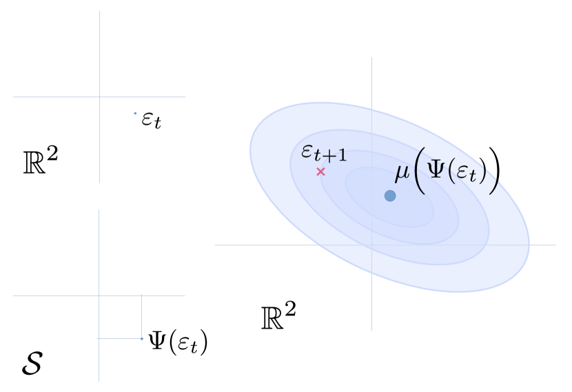
Figure 2: Shock Distribution.

The transition kernel $P_{{\bm{s}},{\bm{s}}^{\prime}}=P\left({\bm{s}}_{t+1}={\bm{s}}^{\prime}\mid{\bm{s}}_{t}={\bm{s}}\right)$ for the Markov chain of states can be written as:

$$P_{{\bm{s}},{\bm{s}}^{\prime}}=\int\limits_{{\bm{s}}^{\prime}\odot\bm{\varepsilon}\succ\mathbf{0}}{\mathcal{N}}\left(\bm{\varepsilon};\bm{\mu}({\bm{s}}),\bm{\Sigma}({\bm{s}})\right)\,d\bm{\varepsilon}.$$ (7)

$P_{{\bm{s}},{\bm{s}}^{\prime}}$ is a valid transition kernel because $\forall{\bm{s}}\in{\mathcal{S}}$, we can show $\sum_{{\bm{s}}^{\prime}\in{\mathcal{S}}}P\left({\bm{s}}^{\prime}\mid{\bm{s}}\right)=1,\because\cup_{{\bm{s}}\ \in{\mathcal{S}}}({\bm{s}}^{\prime}\odot\bm{\varepsilon}\succ\mathbf{0})=\mathbb{R}^{nd}$.

The learning capability of mspace is limited by the number of observed samples in comparison to the cardinality of ${\mathcal{S}}_{v}$. Conceptually, this scenario can be likened to having $|{\mathcal{S}}_{v}|$ buckets, each with a capacity of $M$. In this analogy, $T$ balls are distributed among these buckets. When $|{\mathcal{S}}_{v}|$ is large, each bucket is expected to receive fewer balls. Consequently, the mean-covariance estimates rely on a limited set of samples, potentially impacting the accuracy and reliability of the learned information.

3 RELATED WORKS

3.1 Hidden Markov Model

We can view our model in the framework of an autoregressive hidden Markov model (HMM) (Murphy, 2002), where the current observation (shock) can be sampled using the current hidden state and the previous observation, i.e., $\bm{\varepsilon}_{t}\sim p(\bm{\varepsilon}_{t}|{\bm{s}}_{t},\bm{\varepsilon}_{t-1})$. Moreover, in an HMM, the hidden states $\{{\bm{s}}_{t}:\forall t\in\mathbb{N}\}$ form a Markov chain. We can advance the hidden states by a step and write the trigram $\bm{\varepsilon}_{t}\sim p(\bm{\varepsilon}_{t}|{\bm{s}}_{t-1},\bm{\varepsilon}_{t-1})$ which still is an autoregressive HMM (see Fig. 3). In our case, the hidden state and the observation are related through $\Psi$, so we can reduce the trigram to a bigram $\bm{\varepsilon}_{t}\sim p(\bm{\varepsilon}_{t}|{\bm{s}}_{t-1})$.

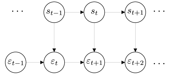
Figure 3: Autoregressive HMM.

We can also compare our method with a simple HMM (see Fig. 4), where the hidden states forms a Markov chain, and the current observation can be sampled from the emission function $f(\cdot)$, i.e., $\bm{\varepsilon}_{t}=f({\bm{s}}_{t-1})\sim p(\bm{\varepsilon}_{t}|{\bm{s}}_{t-1})$. The function $\Omega$ is effectively an emission function. However, in our model the state transition is dictated through ${\bm{s}}_{t}=\Psi\circ\Omega\circ\Psi({\bm{s}}_{t-1})$ instead of sampling from some transition kernel $P({\bm{s}}_{t}|{\bm{s}}_{t-1})$.

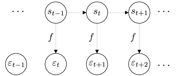
Figure 4: HMM.

3.2 Correlated Time Series Forecasting

Consider a set of $n$ nodes, each generating $d$-dimensional time series. The observation from all the nodes together is denoted by the temporal matrix ${\bm{X}}_{t}\in\mathbb{R}^{n\times d}$ for $t\in[T]$. In correlated time series (CTS) the aim is to discern the correlation between the different rows in the same temporal matrix ${\bm{X}}_{t}$, i.e., find out which nodes are correlated and to what extent; this is the spatial correlation. Furthermore, the goal is also to discern the temporal correlation among different temporal observations.

The goal of CTS forecasting (Lai et al., 2023) is to predict ${\bm{X}}_{t^{\prime}}$ from ${\bm{X}}_{t}$ for some $t^{\prime}>t$ by exploiting the spatial and temporal correlation information learnt from previous observations. We can view the CTS as a graph ${\mathcal{G}}_{t}=({\bm{X}}_{t},{\bm{A}})$ where ${\bm{A}}$ is a weighted adjacency matrix whose values represent the strength of spatial correlation among the observations of different nodes. Now, consider two such graphs ${\mathcal{G}}_{t}$ and ${\mathcal{G}}_{t^{\prime}}$ for some $|t^{\prime}-t|$. The edges between the nodes of ${\mathcal{G}}_{t}$ and the nodes in ${\mathcal{G}}_{t^{\prime}}$ can represent the strength of temporal correlation among the nodes separated by $|t^{\prime}-t|$ time steps.

The architecture of existing CTS forecasting methods can be viewed as the stacking of S and T operators (Lai et al., 2023) responsible for learning the spatial and temporal correlation in the CTS, respectively. For the S-operator, the methods employ either a graph convolutional network (GCN) or a Transformer. As for the T-operator, convolutional neural network (CNN), recurrent neural network (RNN) or Transformer can be used.

3.3 Graph Neural Network

A Graph Neural Network (GNN) is a type of neural network that operates on graph-structured data, such as social networks, citation networks, and molecular graphs. GNNs aim to learn node and graph representations by aggregating and transforming information from neighbouring nodes and edges (Wu et al., 2021). GNNs have shown promising results in various applications, such as node classification, link prediction, and graph classification. Based on the existing literature, the GNNs can be broadly categorized into four types: recurrent GNNs, convolutional GNNs, graph autoencoders, and temporal GNNs.

Recursive Graph Neural Networks (RecGNNs) draw inspiration from RNNs and employ a recursive approach to aggregate information from neighbouring nodes (Veličković et al., 2018). RecGNNs are computationally expensive, but they have shown promising results in tasks such as node classification and link prediction.

Convolutional Graph Neural Networks (ConvGNNs) derive their inspiration from CNNs and leverage convolutional filters to acquire node representations from the graph structure (Kipf & Welling, 2017). ConvGNNs are computationally efficient and can handle large-scale graphs, but they may suffer from over-smoothing and loss of structural information.

Graph Autoencoders (GAEs) operate on the principles of variational autoencoders, with the primary objective of acquiring low-dimensional graph representations (Kipf & Welling, 2016; Komodakis, 2019). This is achieved by encoding the graph’s structural characteristics into a latent space and subsequently decoding them to reconstruct the original graph. GAEs can be used for graph generation, anomaly detection, and graph clustering.

Temporal GNN (TGNN) is an extension of GNNs capable of handling temporal graphs (Longa et al., 2023) such as traffic and social networks. The TGNN architecture for node feature regression can be viewed as a neural network encoder-decoder pair $(f_{\theta},g_{\phi})$:

$${\bm{h}}=f_{\theta}\big{(}\{{\mathcal{G}}_{t-m+1},\cdots{\mathcal{G}}_{t}\}\big{)},$$ (8)

$$\{{\mathcal{G}}_{t+1}^{\prime},\cdots{\mathcal{G}}_{t+q}^{\prime}\}=g_{\phi}({\bm{h}}),$$ (9)

where ${\bm{h}}$ is the spatio-temporal embedding of the input graph sequence, and $G_{t}^{\prime}$ represents the output. The parameters $(\theta,\phi)$ are trained to minimize the difference between the true sequence $\{{\mathcal{G}}_{t+1},\cdots{\mathcal{G}}_{t+q}\}$ and the predicted sequence $\{{\mathcal{G}}_{t+1}^{\prime},\cdots{\mathcal{G}}_{t+q}^{\prime}\}$.

There are two main approaches to implementing TGNNs: model evolution and embedding evolution. In model evolution, the parameters of a static GNN are updated over time to capture the temporal dynamics of the graph. This is achieved by adapting the parameters of the GNN to the changing graph structure and node features. In embedding evolution, the GNN parameters remain fixed, and the node and edge embeddings are updated over time to learn the evolving graph structure and node features.

4 EVALUATION

4.1 Datasets

In Table 1, we list the datasets commonly utilised in the literature for single and multi-step node feature forecasting.

Table 1: Real world datasets for single and multi-step forecasting.

Name	$n$	${\bm{x}}$	time-step	$T$
tennis	1,000	# tweets	1 hour	120
wikimath	1,068	# visits	1 day	731
pedalme	15	# deliveries	1 week	35
cpox	20	# cases	1 week	520
PEMS03	358	flow	5 min	26,208
PEMS04	307	flow	5 min	16,992
PEMS07	883	flow	5 min	28,224
PEMS08	170	flow	5 min	17,856
PEMSBAY	325	speed	5 min	52,116
METRLA	207	speed	5 min	34,272

4.2 Synthetic Dataset

In traffic datasets, seasonality outweighs inter-nodal correlation, making it challenging to assess the efficacy of a TGL algorithm. To address this limitation, we construct a synthetic dataset where node features evolve in concert with the features of their neighbours. The process for generating synthetic datasets in described in Algorithm 2.

We simulate a time series dataset ${{\bm{x}}_{t}}$ based on a given graph ${\mathcal{G}}=({\mathcal{V}},{\mathcal{E}})$ and a set of input parameters. The input includes the graph with nodes ${\mathcal{V}}$ and edges ${\mathcal{E}}$, the dimension $d$ of the data, and various parameters for the data generation process. These parameters encompass the range of mean and variance values, initial data point characteristics, periodicity of a secondary signal, and the associated mean and variance. The algorithm initiates by generating a binary vector $\bm{\varepsilon}_{0}$ following a Bernoulli distribution and the initial data point ${\bm{x}}_{0}$ from a multivariate normal distribution. It then iterates over time steps $0<t<T$ to create the temporal sequence. For each time step, it samples a binary vector ${\bm{s}}_{t-1}$ and checks if it is part of the set ${\mathcal{S}}$. If not, it adds ${\bm{s}}_{t-1}$ to ${\mathcal{S}}$ and initialises mean and covariance matrix parameters from specified ranges. The algorithm generates shock $\bm{\varepsilon}_{t}$ by sampling from a multivariate normal distribution (step 12), and then updates the data point ${\bm{x}}_{t}$ (step 13).

Algorithm 2 Synthetic Data Generator

0:  ${\mathcal{G}}=({\mathcal{V}},{\mathcal{E}})$, $d,\mu_{\min},\mu_{\max},\sigma^{2}_{\min},\sigma^{2}_{\max}$, $\mu_{0},\sigma^{2}_{0}$, $\tau,\mu_{\tau},\sigma^{2}_{\tau}$

1:  $\bm{\varepsilon}_{0}\sim{\rm Bernoulli}^{nd}\left(\frac{1}{2}\right)$

2:  ${\bm{x}}_{0}\sim{\mathcal{N}}({\bm{x}};\mu_{0}\bm{1},\sigma^{2}_{0}{\bm{I}})$

3:  for  $t\in[T]$ do

4:     ${\bm{s}}_{t-1}\leftarrow\Psi(\bm{\varepsilon}_{t-1})$

5:     if  ${\bm{s}}_{t-1}\notin{\mathcal{S}}$  then

6:        ${\mathcal{S}}\leftarrow{\mathcal{S}}\cup\{{\bm{s}}_{t-1}\}$

7:        $\bm{\mu}({\bm{s}}_{t-1})\sim{\rm Uniform}^{nd}(\mu_{\min},\mu_{\max})$

8:        $\bm{\Sigma}\sim{\rm Uniform}^{nd\times nd}(\sigma^{2}_{\min},\sigma^{2}_{\max})$

9:        $\bm{\Sigma}\leftarrow\frac{1}{2}\left(\bm{\Sigma}+\bm{\Sigma}^{\top}\right)$

10:        $\bm{\Sigma}({\bm{s}}_{t-1})\leftarrow\bm{\Sigma}\odot{\bm{A}}_{\bm{\Sigma}}$

11:     end if

12:     $\bm{\varepsilon}_{t}\sim{\mathcal{N}}(\bm{\varepsilon};\bm{\mu}({\bm{s}}_{t-1}),\bm{\Sigma}({\bm{s}}_{t-1}))$

13:     ${\bm{x}}_{t}={\bm{x}}_{t-1}+\bm{\varepsilon}_{t}$

14:  end for

15:  if $\tau>0$ then

16:     ${\bm{y}}_{t}\sim{\mathcal{N}}({\bm{y}};\mu_{\tau}\bm{1},\sigma^{2}_{\tau}{\bm{I}})\quad\forall t\in[\tau]$

17:     ${\bm{x}}_{t}\leftarrow{\bm{x}}_{t}+{\bm{y}}_{t\,{\rm mod}\,\tau}\quad\forall t\in[T]$

18:  end if

The covariance matrix $\bm{\Sigma}({\bm{s}})$ is masked by ${\bm{A}}_{\Sigma}$ which is the Kronecker product of of the graph adjacency matrix ${\bm{A}}$ and an all-one square matrix $\bm{1}_{d\times d}$ (step 10). If $\tau>0$, the data has some degree of periodicity which is introduced by the random signal ${\bm{y}}$ which is tiled repeatedly (step 17). The output is a synthetic time series dataset ${{\bm{x}}_{t}}$, reflecting the specified graph structure and temporal dynamics based on the provided parameters.

4.3 Baselines

The baselines used for single and multi-step forecasting are listed in Table 2.

Table 2: Baselines.

Baseline	Reference
ARIMA	(Box & Pierce, 1970)
DCRNN	(Li et al., 2017)
TGCN	(Zhao et al., 2019)
EGCN-H	(Pareja et al., 2020)
EGCN-O	(Pareja et al., 2020)
DynGESN	(Micheli & Tortorella, 2022)
GWNet	(Wu et al., 2019)
STGODE	(Fang et al., 2021)
FOGS	(Rao et al., 2022)
GRAM-ODE	(Liu et al., 2023)
LightCTS	(Lai et al., 2023)
Kalman	(Welch, 1997)

Since mspace is a state-space algorithm, we also use the Kalman filter (Welch, 1997) as a baseline. We introduce four variants of the Kalman filter: (i) Kalman-${\bm{x}}$, (ii) Kalman-$\bm{\varepsilon}$, (iii) Kalman-${\bm{x}}$I, and (iv) Kalman-$\bm{\varepsilon}$I. Kalman-${\bm{x}}$ operates on the node features of all the nodes at once, i.e., a single hidden state is generated for all the nodes in the graph. Similarly, Kalman-$\bm{\varepsilon}$ operates on the shocks instead of the features. In contrast to the first two variants, Kalman-${\bm{x}}$I, and Kalman-$\bm{\varepsilon}$I operate independently on each node. The implementation details of the Kalman filter are provided in Appendix B.

4.4 Error Metrics

The root mean squared error (RMSE) of $q$ consecutive predictions for all the nodes is:
$\displaystyle\textrm{RMSE}(q)\triangleq\mathbb{E}_{t}\left[\sqrt{\frac{1}{ndq}\sum_{v\in{\mathcal{V}}}\sum_{i\in[q]}\left\lVert\sum_{j\in[i]}\bm{\varepsilon}_{t+j}(v)-\hat{\bm{\varepsilon}}_{t+j}^{[{\mathcal{U}}_{v}]}(v)\right\rVert_{2}^{2}}\right].$

The mean absolute error (MAE) of $q$ consecutive predictions for all the nodes is:
$\displaystyle\textrm{MAE}(q)\triangleq\frac{1}{ndq}\mathbb{E}_{t}\left[\sum_{v\in{\mathcal{V}}}\sum_{i\in[q]}\left\lVert\sum_{j\in[i]}\bm{\varepsilon}_{t+j}(v)-\hat{\bm{\varepsilon}}_{t+j}^{[{\mathcal{U}}_{v}]}(v)\right\rVert_{1}\right].$

5 RESULTS

5.1 Single-step Forecasting

In Table 3, we have single-step forecasting RMSE results for various models with training ratio equal to $0.9$. These results offer insights into the model performance, with bold indicating the best performance and underlined indicating the second-best performance.

Table 3: Single-step forecasting RMSE.

	tennis	wikimath	pedalme	cpox
DynGESN	150.41	906.85	1.25	0.95
DCRNN	155.43	1108.87	1.21	1.05
EGCN-H	155.44	1118.55	1.19	1.06
EGCN-O	155.43	1137.68	1.2	1.07
TGCN	155.43	1109.99	1.22	1.04
LightCTS	199.04	319.47	1.58	0.84
GRAM-ODE	206.50	484.90	0.99	0.98
STGODE	172.16	279.87	0.91	0.83
mspace-S$\mu$	105.32	563.69	0.86	1.58
mspace-S${\mathcal{N}}$	117.23	725.42	1.35	2.11
Kalman-${\bm{x}}$I	73.01	792.6	0.66	1.42
Kalman-$\bm{\varepsilon}$I	7.5K	64K	1.79	10.2

We make the following observations from Table 3:

• DCRNN, ECGN, and TGCN exhibit similar performance across all datasets, which may be attributed to their use of convolutional GNNs for spatial encoding.

• Kalman-$\bm{\varepsilon}$I performs poorly across all datasets, indicating challenges in establishing a state-space relation for shocks. In contrast, Kalman-${\bm{x}}$I performs notably well, outperforming other methods on tennis and pedalme datasets.

• The RMSE of mspace-S$\mu$ is lower than the RMSE of mspace-S${\mathcal{N}}$ for all datasets. This can be explained as follows: Let us assume that ${\bm{x}}\sim p({\bm{x}})={\mathcal{N}}({\bm{x}};\bm{\mu},\bm{\Sigma})$, then in mspace-S$\mu$, the RMSE is of the form: $\mathbb{E}_{{\bm{x}}\sim p}[\left\lVert{\bm{x}}-\mathbb{E}[{\bm{x}}]\right\rVert]\leq\sqrt{{\rm tr}(\bm{\Sigma})}$. However, for mspace-S${\mathcal{N}}$ the RMSE is bounded by: $\mathbb{E}_{{\bm{x}},{\bm{x}}^{\prime}\sim p}[\left\lVert{\bm{x}}-{\bm{x}}^{\prime}\right\rVert]\leq\sqrt{2{\rm tr}(\bm{\Sigma})}$. This suggests that $\mu$-sampling is good for forecasting when the objective is to minimize the RMSE, whereas ${\mathcal{N}}$-sampling is better if the goal is sample generation.

• For wikimath and cpox, STGODE shows the best performance, followed by LightCTS and GRAM-ODE, potentially due to a higher number of training samples available which improve generalisation. The light-weight methods such as Kalman-${\bm{x}}$I and mspace exploit the unavailability of enough training samples and perform better on tennis and pedalme.

• mspace-S$\mu$ achieves a balanced performance between TGNN models and Kalman-${\bm{x}}$I across all datasets except for cpox. The subpar performance of mspace-S* on the cpox dataset may be attributed to the prominent temporal trend in the data, given that it represents the weekly count of chickenpox cases over a period of ten years.

• The parameter estimation process for mspace is relatively straightforward and faster compared to Kalman. Additionally, the performance of a Kalman filter is contingent on the number of iterations used for parameter optimisation, serving as a crucial hyper-parameter.

• mspace proves useful in scenarios with limited training samples, where deploying a heavy NN-based model may be impractical.

Next, we check the performance of the models on the four datasets for different values of training ratio which is presented in Fig. 5. Ideally the RMSE should decrease with increasing training ratio. However, we see an opposite trend for tennis and pedalme datasets across all models. This could be because these are relatively smaller datasets and do not allow the NN-based models to learn effectively. The dataset wikimath is relatively larger, and the RMSE vs training ratio trend is ideal, whereas for cpox the RMSE for all the models remain fairly consistent with increasing training ratio.

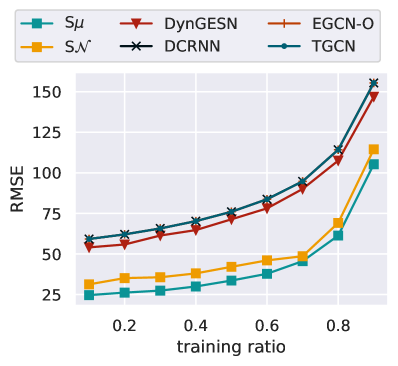
(a) tennis

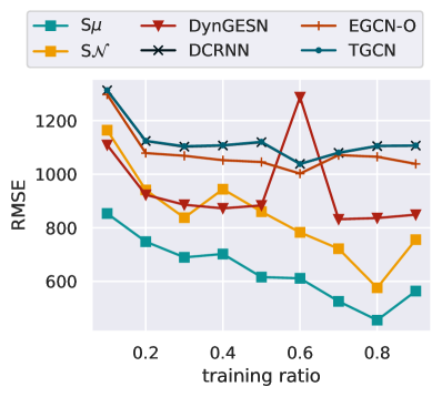
(b) wikimath

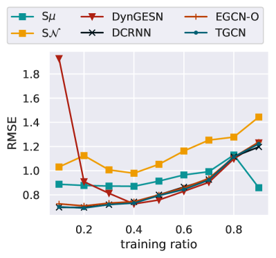
(c) pedalme

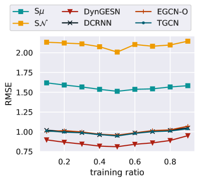
(d) cpox

Figure 5: The RMSE values achieved by different models across 4 datasets as the training split ratio varies.

5.2 Multi-step Forecasting

In Table 4, we have multistep-step forecasting ($q=12$) RMSE results for various models across different traffic datasets with training ratio equal to $0.7$. For mspace-T$\mu$, we set the time period to a week. To better understand the models’ performance, we plot the RMSE against the size of the datasets in Fig. 6.

Table 4: Multi-step traffic forecasting RMSE.

	PEMS03	PEMS04	PEMS07	PEMS08	PEMSBAY	METRLA
GRAM-ODE	26.40	31.05	34.42	25.17	3.34	6.64
STGODE	27.84	32.82	37.54	25.97	4.89	7.37
DCRNN	30.31	38.12	38.58	27.83	4.74	7.60
ARIMA	47.59	48.80	59.27	44.32	6.50	13.23
GWNet	32.94	39.70	42.78	31.05	4.85	7.81
LightCTS	-	30.14	-	23.49	4.32	7.21
FOGS	24.09	31.33	33.96	24.09	-	-
mspace-S$\mu$	36.51	18.85	54.39	14.61	5.14	10.64
mspace-T$\mu$	26.53	13.49	38.63	10.35	3.65	9.22
Kalman-${\bm{x}}$I	45.38	33.75	64.95	27.40	5.71	13.97
Kalman-$\bm{\varepsilon}$I	749	818	2313	460	50.2	127.1

Based on the data presented in Table 4 and the trends observed in Figure 6, the following remarks can be made:

• mspace-T$\mu$ consistently demonstrates superior performance compared to mspace-S$\mu$ across all six traffic datasets, underscoring the prevalence of temporal auto-correlation over spatial cross-correlation within these datasets.

• With the exception of METRLA, mspace-T$\mu$ performs competitively and even surpasses state-of-the-art methods on PEMS04 and PEMS08.

• Kalman-${\bm{x}}$I fails to outperform mspace-*$\mu$, contrary to its success in single-step forecasting. Furthermore, its performance aligns closely with ARIMA, which consistently under-performs across all datasets in single and multi-step forecasting.

• For datasets with more than 25K samples, the RMSE of mspace-S$\mu$ is notably lower-bounded by GWNet.

• The RMSE of mspace-S$\mu$ is upper-bounded by $\min(\texttt{Kalman-${\bm{x}}$I},\texttt{ARIMA})$ for all datasets.

• Similar trends can be seen for MAE values (Table 5).

• The performance of mspace-S$\mu$ and mspace-T$\mu$ remains consistently robust across datasets with varying amount of training samples. Therefore, employing mspace is particularly advantageous in scenarios where the available number of samples is limited.

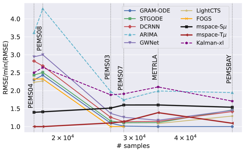
Figure 6: Comparative RMSE of models in multi-step forecasting.

Table 5: Multi-step traffic forecasting MAE.

	PEMS03	PEMS04	PEMS07	PEMS08	PEMSBAY	METRLA
GRAM-ODE	15.72	19.55	21.75	16.05	1.67	3.44
STGODE	16.50	20.84	22.99	16.81	2.30	3.75
DCRNN	18.18	24.70	25.30	17.86	2.07	3.60
ARIMA	33.51	33.73	38.17	31.09	3.38	6.90
GWNet	19.85	25.45	26.85	19.13	1.95	3.53
LightCTS	-	18.79	-	14.63	1.89	3.42
FOGS	15.06	19.35	20.62	14.92	-	-
mspace-S$\mu$	26.43	13.25	38.83	10.36	3.04	7.13
mspace-T$\mu$	18.31	8.70	24.02	6.33	2.07	6.14
Kalman-${\bm{x}}$I	33.21	15.26	48.01	12.40	3.87	10.7
Kalman-$\bm{\varepsilon}$I	619	709	1988	399	43.1	109

In Table 6, we present the RMSE of multi-step forecasting on the synthetic datasets SYN02 and SYN03. The details of these datasets can be found in Appendix C. In both datasets, mspace-S$\mu$ performs consistently well compared to Kalman-$\bm{\varepsilon}$I, which performs well on SYN03 but not on SYN02. Among the GNN-based methods, GRAM-ODE has the highest RMSE, contrary to its performance on the traffic datasets. The GNN-based models have high variance in RMSE compared to state-space models like mspace and Kalman. This behaviour is expected as synthetic dataset generation itself follows a state-space model.

Table 6: Performance on synthetic datasets: RMSE.

	SYN02	SYN03
mspace-S$\mu$	$\mathbf{294.99}\pm\mathbf{8.81}$	$793.41\pm 5.86$
mspace-S${\mathcal{N}}$	$395.33\pm 3.24$	$793.93\pm 5.73$
LightCTS	$334.59\pm 79.01$	$769.34\pm 196.6$
STGODE	$420.25\pm 52.17$	$830.63\pm 127$
GRAM-ODE	$853.77\pm 340.45$	$1382.48\pm 80.78$
Kalman-${\bm{x}}$I	$776.75\pm 30.38$	$785.7\pm 8.95$
Kalman-$\bm{\varepsilon}$I	$390.45\pm 3.54$	$\mathbf{782.6}\pm\mathbf{6.5}$

As mspace generates predictions iteratively, with each prediction at time $t+q$ depending on the preceding prediction at time $t+q-1$, errors propagate throughout the forecasting steps. Consequently, an increase in the total error is expected as the number of forecasting steps increases. We formalise this scaling in the following lemma 5.1 and demonstrate it visually in Fig. 7 for different flavours of mspace.

Lemma 5.1.

The RMSE of $q$-step iterative prediction by mspace is upper bounded by ${\mathcal{O}}(q)$.

Proof.

See Appendix D. ∎

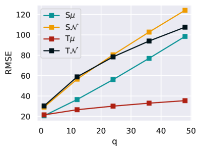
(a) PEMS03

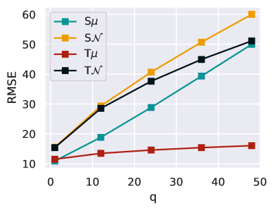
(b) PEMS04

(c) PEMS07

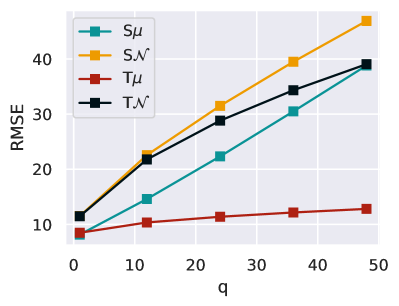
(d) PEMS08

Figure 7: RMSE vs. number of forecast steps.

Lastly, we outline the distinctions between mspace and the baseline models, underscoring the specific contributions of mspace to the literature on node feature forecasting.

• Unlike GNN-based models forecasting node features for $q=12$ steps relying on $m=12$ previous steps, mspace achieves comparable results using only $m=2$ previous steps.

• mspace is an online learning algorithm capable of real-time adaptation, while all the baseline models are offline and necessitate training beforehand.

• Unlike the baseline models that can only return deterministic output, mspace is capable of generating both deterministic ($\mu$) and probabilistic (${\mathcal{N}}$) outputs.

• Baseline models leverage edge weights for predictions, harnessing additional information on node correlations. In contrast, mspace operates with binary edges, achieving comparable prediction accuracy with less information. The influence of edge weights on TGL is further investigated in Appendix E.

• The hidden states in the GNN-based models or Kalman filters cannot be interpreted numerically. However, the state function definition in mspace provides an interpretable understanding of the algorithm. which is a step towards interpretable TGL.

6 CONCLUSION

In conclusion, our proposed algorithm, mspace, performs at par with the latest GNN-based models across various temporal graph datasets. As an online learning algorithm, mspace is adaptive to changes in data distribution and is suitable for deployment in scenarios where training samples are limited. Furthermore, the operation of mspace is numerically interpretable, unlike black-box deep learning models, which marks a progression towards explainable temporal graph learning.

In addition to the algorithm, we introduced a synthetic temporal graph generator in which the features of the nodes evolve with the influence of their neighbours. These synthetic datasets can serve as a valuable resource for benchmarking algorithms.

The proposed algorithm works with temporal graphs with a fixed structure. Moreover, the edge weights are considered binary, scalar and static. We can extend mspace to exploit the spatiotemporal information conveyed by dynamic real-valued edge weight vectors in a way which remains numerically and logically interpretable. The state functions defined are either spatial or seasonal. In the future, we can create a state function which is both spatial and seasonal. We can perform edge feature forecasting by feeding the corresponding line graph (Harary & Norman, 1960) to mspace. We can also test the efficacy of mspace at performing node classification in temporal graphs.

Appendix A Computational Complexity of mspace

We denote the computational complexity operator as $\mathfrak{C}(\cdot)$, the argument of which is an algorithm or part of an algorithm.

A.1 mspace-S${\mathcal{N}}$

Algorithm 3 mspace-S${\mathcal{N}}$

0:  ${\mathcal{G}}=({\mathcal{V}},{\mathcal{E}},{\bm{X}})$, $r\in[0,1)$, $q,M,K,\tau_{0}\in\mathbb{N}$

0:  $\hat{\bm{\varepsilon}}_{t}(v),\quad\forall v\in{\mathcal{V}},t\in[\lfloor r\cdot T\rfloor,T]$

1:  $\bm{\varepsilon}_{t}(v)\leftarrow{\bm{x}}_{t}(v)-{\bm{x}}_{t-1}(v),\quad\forall v\in{\mathcal{V}},\,t\in[T]$ Offline training $(\mathsf{A})$:

2:  for $t\in[\lfloor r\cdot T\rfloor]$ do

3:     for $v\in{\mathcal{V}}$ do

4:        $\displaystyle{\bm{s}}_{t}^{[{\mathcal{U}}_{v}]}\leftarrow\Psi\left(\bm{\varepsilon}_{t}^{[{\mathcal{U}}_{v}]}\right)$ $\lx@algorithmic@hfill\triangleright\,$$\sum_{v\in{\mathcal{V}}}d|{\mathcal{U}}_{v}|$

5:        ${\mathcal{S}}_{v}\leftarrow{\mathcal{S}}_{v}\cup\left\{{\bm{s}}_{t}^{[{\mathcal{U}}_{v}]}\right\}$ $\lx@algorithmic@hfill\triangleright\,$$n$

6:        ${\mathcal{Q}}_{v}\left({\bm{s}}_{t}^{[{\mathcal{U}}_{v}]}\right)\leftarrow$ append $\bm{\varepsilon}_{t+1}^{[{\mathcal{U}}_{v}]}$ $\lx@algorithmic@hfill\triangleright\,$$n$

7:     end for

8:  end for

9:  $\bm{\mu}_{v}({\bm{s}})\leftarrow{\rm mean}({\mathcal{Q}}_{v}({\bm{s}})),\quad\forall s\in{\mathcal{S}}_{v},v\in{\mathcal{V}}$ $\lx@algorithmic@hfill\triangleright\,$$\sum_{v\in{\mathcal{V}}}d|{\mathcal{U}}_{v}||{\mathcal{S}}_{v}|M$

10:  $\bm{\Sigma}_{v}({\bm{s}})\leftarrow{\rm covariance}({\mathcal{Q}}_{v}({\bm{s}})),\quad\forall s\in{\mathcal{S}}_{v},v\in{\mathcal{V}}$ $\lx@algorithmic@hfill\triangleright\,$$\sum_{v\in{\mathcal{V}}}(d|{\mathcal{U}}_{v}|)^{2}|{\mathcal{S}}_{v}|M$ Online learning $(\mathsf{B})$:

11:  for $t\in[\lfloor r\cdot T\rfloor,T-q]$ do

12:     for $v\in{\mathcal{V}}$ do

13:        $\displaystyle{\bm{s}}_{t}^{[{\mathcal{U}}_{v}]}\leftarrow\Psi\left(\bm{\varepsilon}_{t}^{[{\mathcal{U}}_{v}]}\right)$ $\lx@algorithmic@hfill\triangleright\,$$\sum_{v\in{\mathcal{V}}}d|{\mathcal{U}}_{v}|$

14:        $\displaystyle{\bm{s}}^{*}\leftarrow\arg\min_{{\bm{s}}\in{\mathcal{S}}_{v}}\left\lVert{\bm{s}}-{\bm{s}}_{t}^{[{\mathcal{U}}_{v}]}\right\rVert$ $\lx@algorithmic@hfill\triangleright\,$$\sum_{v\in{\mathcal{V}}}d|{\mathcal{U}}_{v}||{\mathcal{S}}_{v}|$

15:        $\hat{\bm{\varepsilon}}_{t+1}^{[{\mathcal{U}}_{v}]}\sim{\mathcal{N}}(\bm{\varepsilon};\bm{\mu}_{v}({\bm{s}}^{*}),\bm{\Sigma}_{v}({\bm{s}}^{*}))$ $\lx@algorithmic@hfill\triangleright\,$$\sum_{v\in{\mathcal{V}}}(|{\mathcal{U}}_{v}|d)^{3}$

16:        for $k\in[2,q]$ do

17:           $\displaystyle{\bm{s}}^{*}\leftarrow\arg\min_{{\bm{s}}\in{\mathcal{S}}_{v}}\left\lVert{\bm{s}}-\Psi\left(\hat{\bm{\varepsilon}}_{t+k-1}^{[{\mathcal{U}}_{v}]}\right)\right\rVert$ $\lx@algorithmic@hfill\triangleright\,$$(q-1)\times\sum_{v\in{\mathcal{V}}}d|{\mathcal{U}}_{v}|(1+|{\mathcal{S}}_{v}|)$

18:           $\hat{\bm{\varepsilon}}_{t+k}^{[{\mathcal{U}}_{v}]}\sim{\mathcal{N}}(\bm{\varepsilon};\bm{\mu}_{v}({\bm{s}}^{*}),\bm{\Sigma}_{v}({\bm{s}}^{*}))$ $\lx@algorithmic@hfill\triangleright\,$$(q-1)\times\sum_{v\in{\mathcal{V}}}(|{\mathcal{U}}_{v}|d)^{3}$

19:        end for

20:        $\hat{\bm{\varepsilon}}_{t+k}(v)\leftarrow\hat{\bm{\varepsilon}}_{t+k}^{[{\mathcal{U}}_{v}]}(v),\quad\forall k\in[q]$

21:        Update ${\mathcal{S}}_{v},{\mathcal{Q}}_{v}$ $\lx@algorithmic@hfill\triangleright\,$$2n$

22:        Update $\bm{\mu}_{v}({\bm{s}}),\bm{\Sigma}_{v}({\bm{s}}),\quad\forall{\bm{s}}\in{\mathcal{S}}_{v}$ $\lx@algorithmic@hfill\triangleright\,$$\sum_{v\in{\mathcal{V}}}(d|{\mathcal{U}}_{v}|+d^{2}|{\mathcal{U}}_{v}|^{2})|{\mathcal{S}}_{v}|M$

23:     end for

24:  end for

Computational complexity of offline training:

$$\mathfrak{C}(\mathsf{A})={\mathcal{O}}\left(\underbrace{\lfloor rT\rfloor d\sum_{v}|{\mathcal{U}}_{v}|}_{[4]}+\underbrace{\lfloor rT\rfloor 2n}_{[5],[6]}+\underbrace{dM\sum_{v}|{\mathcal{U}}_{v}||{\mathcal{S}}_{v}|}_{[9]({\rm mean})}+\underbrace{d^{2}M\sum_{v}|{\mathcal{U}}_{v}|^{2}|{\mathcal{S}}_{v}|}_{[10]({\rm covariance})}\right).$$ (10)

Computational complexity of online learning:

$$\mathfrak{C}(\mathsf{B})={\mathcal{O}}\left(\sum_{t=\lceil rT\rceil}^{T-q}\left\{\underbrace{dq\sum_{v}|{\mathcal{U}}_{v}|}_{[13],[17]}+\underbrace{dq\sum_{v}|{\mathcal{U}}_{v}||{\mathcal{S}}_{v}|}_{[14],[17]}+\underbrace{d^{3}q\sum_{v}|{\mathcal{U}}_{v}|^{3}}_{[15],[18]({\rm sampling})}+\underbrace{2n}_{[21]}+\underbrace{dM\sum_{v}|{\mathcal{U}}_{v}||{\mathcal{S}}_{v}|}_{[22]({\rm mean})}+\underbrace{d^{2}M\sum_{v}|{\mathcal{U}}_{v}|^{2}|{\mathcal{S}}_{v}|}_{[22]({\rm covariance})}\right\}\right).$$ (11)

The following conditions can be imposed on $|{\mathcal{U}}_{v}|$ and $|{\mathcal{S}}_{v}|$:

$$|{\mathcal{U}}_{v}|\leq b<n,$$ (12)

$$|{\mathcal{S}}_{v}|\leq 2^{|{\mathcal{U}}_{v}|d}\leq 2^{bd}<2^{nd},$$ (13)

$$\sum_{v\in{\mathcal{V}}}|{\mathcal{S}}_{v}|\leq t$$ (14)

Based on the above inequalities, we can write $\sum_{v\in{\mathcal{V}}}|{\mathcal{S}}_{v}|\leq\min\{t,n2^{bd}\}$. For large graphs we can safely assume that $\sum_{v\in{\mathcal{V}}}|{\mathcal{S}}_{v}|\leq t$. Furthermore, $\lfloor rT\rfloor\approx rT$. Therefore, equation 10 can be written as:

$$\mathfrak{C}(\mathsf{A})={\mathcal{O}}\left(dbnrT+2nrT+dbMrT+d^{2}b^{2}MrT\right)\implies{\mathcal{O}}\Big{(}(dbn+d^{2}b^{2}M)\cdot rT\Big{)}.$$

We can write equation 11 as:

$$\mathfrak{C}(\mathsf{B})= {\mathcal{O}}\left(\sum_{t=\lceil rT\rceil}^{T-q}qdbn+qd^{3}b^{3}n+2n+db(q+M)\cdot t+d^{2}b^{2}M\cdot t\right)$$

$$\implies {\mathcal{O}}\left(\sum_{t=\lceil rT\rceil}^{T-q}qd^{3}b^{3}n+(db(q+M)+d^{2}b^{2}M)\cdot t\right)$$

$$\stackrel{{\scriptstyle T\gg q}}{{\implies}} {\mathcal{O}}\left((1-r)T\cdot qd^{3}b^{3}n+(1-r^{2})T^{2}\cdot d^{2}b^{2}M\right).$$

A.2 mspace-S$\mu$

In mspace-S$\mu$, the sampling steps (15) and (18) are replaced with $\hat{\bm{\varepsilon}}_{t}^{[{\mathcal{U}}_{v}]}\leftarrow\bm{\mu}({\bm{s}}^{*})$ which has a computational complexity of ${\mathcal{O}}(d|{\mathcal{U}}_{v}|)$. Moreover, the covariance calculation steps are removed.

$$\mathfrak{C}(\mathsf{A})={\mathcal{O}}\left(\lfloor rT\rfloor d\sum_{v}|{\mathcal{U}}_{v}|+\lfloor rT\rfloor 2n+dM\sum_{v}|{\mathcal{U}}_{v}||{\mathcal{S}}_{v}|\right)\implies{\mathcal{O}}\left(dbnrT\right).$$

$$\mathfrak{C}(\mathsf{B})= {\mathcal{O}}\left(\sum_{t=\lceil rT\rceil}^{T-q}\left\{dq\sum_{v}|{\mathcal{U}}_{v}|+dq\sum_{v}|{\mathcal{U}}_{v}||{\mathcal{S}}_{v}|+\underbrace{dq\sum_{v}|{\mathcal{U}}_{v}|}_{({\rm sampling})}+2n+dM\sum_{v}|{\mathcal{U}}_{v}||{\mathcal{S}}_{v}|\right\}\right)$$

$$\implies{\mathcal{O}}\left(\sum_{t=\lceil rT\rceil}^{T-q}2qdbn+2n+db(q+M)\cdot t\right)\implies{\mathcal{O}}\Big{(}(1-r)T\cdot qdbn+(1-r^{2})T^{2}\cdot db(q+M)\Big{)}.$$

A.3 mspace-T${\mathcal{N}}$

The number of states that any node can have is limited to $\tau_{0}$ in mspace-T*, and we can write $|{\mathcal{S}}_{v}|\leq\tau_{0},\,\forall v\in{\mathcal{V}}$. Moreover, the state $\Psi(t)$ calculation has computational complexity of ${\mathcal{O}}(1)$.

$$\mathfrak{C}(\mathsf{A})= {\mathcal{O}}\left(\lfloor rT\rfloor\sum_{v}1+\lfloor rT\rfloor 2n+dM\sum_{v}|{\mathcal{U}}_{v}||{\mathcal{S}}_{v}|+d^{2}M\sum_{v}|{\mathcal{U}}_{v}|^{2}|{\mathcal{S}}_{v}|\right)$$

$$\implies{\mathcal{O}}\left(3nrT+dbMn\tau_{0}+d^{2}b^{2}Mn\tau_{0}\right)\implies{\mathcal{O}}\left(nrT+d^{2}b^{2}Mn\tau_{0}\right).$$

$$\mathfrak{C}(\mathsf{B})={\mathcal{O}}\left(\sum_{t=\lceil rT\rceil}^{T-q}\left\{q\sum_{v}1+dq\sum_{v}|{\mathcal{U}}_{v}||{\mathcal{S}}_{v}|+d^{3}q\sum_{v}|{\mathcal{U}}_{v}|^{3}+2n+dM\sum_{v}|{\mathcal{U}}_{v}||{\mathcal{S}}_{v}|+d^{2}M\sum_{v}|{\mathcal{U}}_{v}|^{2}|{\mathcal{S}}_{v}|\right\}\right)$$

$$\implies{\mathcal{O}}\left(\{q+dbq\tau_{0}+qd^{3}b^{3}+2+dbM\tau_{0}+d^{2}b^{2}M\tau_{0}\}\cdot n(1-r)T\right)\implies{\mathcal{O}}\Big{(}(1-r)Tn\cdot(d^{2}b^{2}M\tau_{0}+qd^{3}b^{3})\Big{)}.$$

A.4 mspace-T$\mu$

The conditions from mspace-T${\mathcal{N}}$ hold true, and $|{\mathcal{U}}_{v}|$ loses its significance as we deal with the mean only, therefore, we can write $|{\mathcal{U}}_{v}|=1$.

$$\mathfrak{C}(\mathsf{A})={\mathcal{O}}\left(\lfloor rT\rfloor\sum_{v}1+\lfloor rT\rfloor 2n+dM\sum_{v}|{\mathcal{S}}_{v}|\right)\implies{\mathcal{O}}\left(3nrT+dMn\tau_{0}\right)\implies{\mathcal{O}}\left(nrT+dMn\tau_{0}\right).$$

$$\mathfrak{C}(\mathsf{B}) ={\mathcal{O}}\left(\sum_{t=\lceil rT\rceil}^{T-q}\left\{q\sum_{v}1+dq\sum_{v}|{\mathcal{S}}_{v}|+2n+dM\sum_{v}|{\mathcal{S}}_{v}|\right\}\right)$$

$$\implies{\mathcal{O}}\Big{(}\{q+dq\tau_{0}+2+dM\tau_{0}\}\cdot n(1-r)T\Big{)}\implies{\mathcal{O}}\Big{(}(1-r)Tn\cdot d(q+M)\tau_{0}\Big{)}.$$

Since $b\leq n$, we can do asymptotic analysis and obtain $\mathfrak{C}(\mathsf{A})$ and $\mathfrak{C}(\mathsf{B})$ in terms of $n$ and $T$.

	$\mathfrak{C}(\mathsf{A})$	$\mathfrak{C}(\mathsf{B})$
mspace-S${\mathcal{N}}$	${\mathcal{O}}(n^{2}T)$	${\mathcal{O}}(n^{4}T+n^{2}T^{2})$
mspace-S$\mu$	${\mathcal{O}}(n^{2}T)$	${\mathcal{O}}(n^{2}T+nT^{2})$
mspace-T${\mathcal{N}}$	${\mathcal{O}}(nT+n^{3})$	${\mathcal{O}}(n^{4}T)$
mspace-T$\mu$	${\mathcal{O}}(nT)$	${\mathcal{O}}(nT)$

Table 7: computational complexity of different mspace flavours in terms of $n$ and $T$.

Appendix B Implementation of the Kalman Filter

Kalman filter is a state-space model in which a set of observations $\{y_{0},y_{1},\cdots,y_{t},\cdots,y_{T}\}$ is approximated as emissions from an HMM in which the hidden state at time $t$ is denoted as ${\bm{h}}_{t}\in\mathbb{R}^{l}$.

$${\bm{h}}_{0} \sim{\mathcal{N}}(\bm{\mu}_{0},\bm{\Sigma}_{0}),$$ (15)

$${\bm{h}}_{t+1} \sim{\mathcal{N}}({\bm{A}}{\bm{h}}_{t}+{\bm{b}},\bm{\Sigma}),$$ (16)

$${\bm{y}}_{t} \sim{\mathcal{N}}({\bm{C}}{\bm{h}}_{t}+{\bm{d}},\tilde{\bm{\Sigma}}).$$ (17)

Based on how we define ${\bm{y}}_{t}$, we get four different flavours of the Kalman filter suited to our task of node feature forecasting.

Kalman-${\bm{x}}$	${\bm{y}}_{t}={\bm{x}}_{t}$
Kalman-$\bm{\varepsilon}$	${\bm{y}}_{t}=\bm{\varepsilon}_{t}$
Kalman-${\bm{x}}$I	${\bm{y}}_{t}={\bm{x}}_{t}(v)$	$\forall v\in{\mathcal{V}}$
Kalman-$\bm{\varepsilon}$I	${\bm{y}}_{t}=\bm{\varepsilon}_{t}(v)$	$\forall v\in{\mathcal{V}}$

Table 8: Different flavours of Kalman filter.

The set of parameters $\{\bm{\mu}_{0},\bm{\Sigma}_{0},{\bm{A}},{\bm{b}},{\bm{C}},{\bm{d}},\bm{\Sigma},\tilde{\bm{\Sigma}}\}$ are estimated by $\tau$-iteration EM algorithm (Bishop, 2006)[Sec. 13.3.2] after supplying $\lfloor rT\rfloor$ samples $\{{\bm{y}}_{0},{\bm{y}}_{1},\cdots,{\bm{y}}_{\lfloor rT\rfloor}\}$. This is analogous to the offline training procedure of mspace.

For $t>\lfloor rT\rfloor$, we perform prediction. First, we estimate the hidden state ${\bm{h}}_{t}$ by supplying past $q$ observations $\{{\bm{y}}_{t-1+1},\cdots{\bm{y}}_{t-1},{\bm{y}}_{t}\}$. Based on ${\bm{h}}_{t}$ we sample the next $q$ steps $\{y_{t+1},\cdots,y_{t+1}\}$ iteratively using equation 16 and equation 17.

Since the EM algorithm relies on matrix inversion operation which has a complexity of ${\mathcal{O}}((\dim{{\bm{y}}_{t}})^{3})$, the complexity of $\tau$-iteration EM algorithm of Kalman-${\bm{x}}$ and Kalman-$\bm{\varepsilon}$ which is fed $\lfloor rT\rfloor$ observations is ${\mathcal{O}}(\tau rTd^{3}n^{3})$, and that of Kalman-${\bm{x}}$I and Kalman-$\bm{\varepsilon}$I is ${\mathcal{O}}(\tau rTd^{3}n)$.

Appendix C Experiment: Impact of Periodicity and Number of Training Samples

We generate datasets through Algorithm 2 by supplying the parameters outlined in Table 9. For each dataset, we create multiple random instances and report the mean and standard deviation of the metrics in the results.

Table 9: Parameters for different synthetic dataset packages.

Dataset	${\mathcal{G}}\sim$	$d$	$T$	$\mu_{\min}$	$\mu_{\max}$	$\sigma_{\min}$	$\sigma_{\max}$	$\mu_{0}$	$\sigma_{0}$	$\tau$	$\mu_{\tau}$	$\sigma_{\tau}$
SYN01	$\mathfrak{G}_{\rm ER}\left(20,0.2\right)$	1	$10^{3}$	$-200$	$200$	$40$	$50$	$2\times 10^{4}$	$5000$	$100$	$100$	$20$
SYN02	$\mathfrak{G}_{\rm ER}\left(20,0.2\right)$	1	$10^{3}$	$-200$	$200$	$40$	$50$	$2\times 10^{4}$	$5000$	0
SYN03	$\mathfrak{G}_{\rm ER}\left(40,0.5\right)$	1	$10^{3}$	$-400$	$400$	$30$	$40$	$10^{4}$	$2000$	0
SYN04	$\mathfrak{G}_{\rm ER}\left(40,0.5\right)$	1	$10^{4}$	$-400$	$400$	$30$	$40$	$10^{4}$	$2000$	0

Table 10: Node feature of five exemplary nodes in each synthetic dataset instance.

SYN01
SYN02
SYN03
SYN04

C.1 Periodicity

The generator parameters for SYN01 and SYN02 are same except for the periodic component added to SYN01 which has a period of $\tau=100$ timesteps consisting of shocks sampled from ${\mathcal{N}}(100,20)$. An algorithm which can exploit the periodic influence in the signal should perform better on SYN01 compared to SYN02. The models which perform worse on periodic dataset are marked red, and the ones that perform better are marked teal.

Table 11: Impact of data periodicity on RMSE achieved by different models.

	SYN01				SYN02			% increase
	mean		std. dev.		mean		std. dev.	$\left(\frac{\texttt{SYN02}-\texttt{SYN01}}{\texttt{SYN01}}\right)$
mspace-S$\mu$	299.18	$\pm$	6.55		294.99	$\pm$	8.81	$-0.63$
mspace-S${\mathcal{N}}$	400.99	$\pm$	3.74		395.33	$\pm$	3.24	$-1.52$
STGODE	420.86	$\pm$	103.29		420.25	$\pm$	52.17	$-9.87$
GRAM-ODE	921.94	$\pm$	537.63		853.77	$\pm$	340.45	$-18.18$
LightCTS	419.43	$\pm$	176.5		334.59	$\pm$	79.01	$-30.6$
Kalman-${\bm{x}}$	776.18	$\pm$	145.82		832.08	$\pm$	137.37	$+5.15$
Kalman-${\bm{x}}$I	781.94	$\pm$	32.35		776.75	$\pm$	30.38	$-0.88$
Kalman-$\bm{\varepsilon}$	396.34	$\pm$	3.43		392.3	$\pm$	2.35	$-1.28$
Kalman-$\bm{\varepsilon}$I	393.76	$\pm$	4.72		390.45	$\pm$	3.54	$-1.13$

C.2 Training Samples

The generator parameters for SYN03 and SYN04 are same except for the total number of samples being ten times more in SYN04. Since we train the models on a fraction of the total dataset, if models perform better on SYN04 compared to SYN03, it would indicate that they are training intensive, and need more samples to infer the predictive trends. On the other hand, if the model performs worse on SYN04, it would indicate that there are scalability issues, or the training caused overfitting. An ideal model is expected to have similar performance on SYN03 and SYN04. The models with ideal behaviour are marked teal, and the models suseptible to overfitting are marked red. Moreover, model(s) that require more training samples are marked violet.

Table 12: Impact of number of training samples on RMSE achieved by different models.

	SYN03				SYN04			% increase
	mean		std. dev.		mean		std. dev.	$\left(\frac{\texttt{SYN04}-\texttt{SYN03}}{\texttt{SYN03}}\right)$
mspace-S$\mu$	793.41	$\pm$	5.86		789.36	$\pm$	3	$-0.86$
mspace-S${\mathcal{N}}$	793.93	$\pm$	5.73		792.61	$\pm$	2.02	$-0.63$
STGODE	830.63	$\pm$	127		931.33	$\pm$	191.87	$+17.29$
GRAM-ODE	1382.48	$\pm$	80.78		1423.93	$\pm$	190.13	$+10.31$
LightCTS	769.34	$\pm$	196.6		998.01	$\pm$	319.72	$+36.42$
Kalman-${\bm{x}}$	1847.42	$\pm$	158.37		4528.49	$\pm$	1138.19	$+182.52$
Kalman-${\bm{x}}$I	785.7	$\pm$	8.95		721.88	$\pm$	1.73	$-8.94$
Kalman-$\bm{\varepsilon}$	786.08	$\pm$	8.44		785	$\pm$	2.1	$-0.93$
Kalman-$\bm{\varepsilon}$I	782.6	$\pm$	6.5		783.36	$\pm$	1.45	$-0.54$

Appendix D Upper Bound on the RMSE of mspace

Lemma.

The RMSE of $q$-step iterative prediction by mspace is upper bounded by ${\mathcal{O}}(q)$.

Proof.

The predicted shock $\bm{\varepsilon}_{t}^{\prime}(v)\sim p\left(\bm{\varepsilon}_{t}^{\prime}(v)\,\Big{|}\,\Psi\left(\bm{\varepsilon}^{\prime[{\mathcal{U}}_{v}]}_{t-1}\right)\right)={\mathcal{N}}\left(\bm{\varepsilon}_{t}^{\prime}(v);\bm{\mu}\left(\Psi\left(\bm{\varepsilon}^{\prime[{\mathcal{U}}_{v}]}_{t-1}\right)\right),\bm{\Sigma}\left(\Psi\left(\bm{\varepsilon}^{\prime[{\mathcal{U}}_{v}]}_{t-1}\right)\right)\right)$ for a node $v\in[n]$. Further, we impose $\bm{\varepsilon}_{t}^{\prime}(v)\perp\!\!\!\!\perp\bm{\varepsilon}_{t}^{\prime}(u)$ for $u\neq v$, following which we can express the shocks of all the nodes as:

$$\bm{\varepsilon}_{t}^{\prime}\triangleq\begin{bmatrix}\bm{\varepsilon}_{t}^{\prime}(1)\\ \vdots\\ \bm{\varepsilon}_{t}^{\prime}(v)\\ \vdots\\ \bm{\varepsilon}_{t}^{\prime}(n)\end{bmatrix}\sim{\mathcal{N}}\left(\bm{\varepsilon}_{t}^{\prime};\begin{bmatrix}\bm{\mu}\left(\Psi\left(\bm{\varepsilon}^{\prime[{\mathcal{U}}_{1}]}_{t-1}\right)\right)\\ \vdots\\ \bm{\mu}\left(\Psi\left(\bm{\varepsilon}^{\prime[{\mathcal{U}}_{v}]}_{t-1}\right)\right)\\ \vdots\\ \bm{\mu}\left(\Psi\left(\bm{\varepsilon}^{\prime[{\mathcal{U}}_{n}]}_{t-1}\right)\right)\end{bmatrix},{\rm diag}\left(\begin{bmatrix}\bm{\Sigma}\left(\Psi\left(\bm{\varepsilon}^{\prime[{\mathcal{U}}_{1}]}_{t-1}\right)\right)\\ \vdots\\ \bm{\Sigma}\left(\Psi\left(\bm{\varepsilon}^{\prime[{\mathcal{U}}_{v}]}_{t-1}\right)\right)\\ \vdots\\ \bm{\Sigma}\left(\Psi\left(\bm{\varepsilon}^{\prime[{\mathcal{U}}_{n}]}_{t-1}\right)\right)\end{bmatrix}\right)\right),$$

where the covariance matrix is a block diagonal matrix. Alternatively, we can write: $\bm{\varepsilon}_{t}^{\prime}\sim p(\bm{\varepsilon}_{t}^{\prime}\mid\Psi(\bm{\varepsilon}_{t-1}^{\prime}),{\bm{A}})$, we encode ${\bm{s}}_{t-1}^{\prime}\triangleq(\Psi(\bm{\varepsilon}_{t-1}^{\prime}),{\bm{A}})$, and express the distribution of $\bm{\varepsilon}_{t}^{\prime}$ as a GMM: $\bm{\varepsilon}_{t}^{\prime}\sim\sum_{{\bm{s}}\in{\mathcal{S}}}\mathbb{I}\{{\bm{s}}_{t-1}^{\prime}={\bm{s}}\}\cdot{\mathcal{N}}\Big{(}\bm{\varepsilon}_{t}^{\prime};\bm{\mu}({\bm{s}}),\bm{\Sigma}({\bm{s}})\Big{)}.$

We assume that the true shocks are Markovian, without imposing a hidden Markov model, or independence between the shocks of different nodes. This way, we approximate $\bm{\varepsilon}_{t}\sim p(\bm{\varepsilon}_{t}\mid\bm{\varepsilon}_{t-1})={\mathcal{N}}(\bm{\varepsilon}_{t};\bm{\mu}(\bm{\varepsilon}_{t-1}),\bm{\Sigma}(\bm{\varepsilon}_{t-1}))$.

The true shocks follow the chain: $\bm{\varepsilon}_{1}\rightarrow\bm{\varepsilon}_{2}\rightarrow\cdots\bm{\varepsilon}_{t-1}\rightarrow\bm{\varepsilon}_{t}\rightarrow\bm{\varepsilon}_{t+1}\rightarrow\cdots\bm{\varepsilon}_{t+j}\cdots\rightarrow\bm{\varepsilon}_{T}$. The states of the predicted shock, on iterative sampling form a chain: ${\bm{s}}_{1}\rightarrow{\bm{s}}_{2}\rightarrow\cdots{\bm{s}}_{t-1}\rightarrow{\bm{s}}_{t}\rightarrow{\bm{s}}_{t+1}\rightarrow\cdots{\bm{s}}_{t+j}\cdots\rightarrow{\bm{s}}_{T}$.

The difference between the true and predicted shocks at time $t$ is $\bm{\varepsilon}_{t}-\bm{\varepsilon}_{t}^{\prime}$, where $\bm{\varepsilon}_{t}\sim{\mathcal{N}}(\bm{\mu}(\bm{\varepsilon}_{t-1}),\bm{\Sigma}(\bm{\varepsilon}_{t-1}))$, and $\bm{\varepsilon}_{t}^{\prime}\sim{\mathcal{N}}(\bm{\mu}({\bm{s}}_{t-1}),\bm{\Sigma}({\bm{s}}_{t-1}))$. Since the sum of two Gaussian r.v.s is also Gaussian, we can write:

$$\bm{\varepsilon}_{t}-\bm{\varepsilon}_{t}^{\prime}\sim{\mathcal{N}}\Big{(}{\bm{z}};\bm{\mu}(\bm{\varepsilon}_{t-1})-\bm{\mu}({\bm{s}}_{t-1}),\bm{\Sigma}(\bm{\varepsilon}_{t-1})+\bm{\Sigma}({\bm{s}}_{t-1})\Big{)}.$$

$$\textrm{MSE}(q)\triangleq\frac{1}{ndq}\mathbb{E}\left[\sum_{i\in[q]}\left\lVert\sum_{j\in[i]}\bm{\varepsilon}_{t+j}-\bm{\varepsilon}_{t+j}^{\prime}\right\rVert^{2}\right]=\frac{1}{ndq}\sum_{i\in[q]}\mathbb{E}\left[\left\lVert\sum_{j\in[i]}\bm{\varepsilon}_{t+j}-\bm{\varepsilon}_{t+j}^{\prime}\right\rVert^{2}\right].$$

$$\sum_{j\in[i]}\bm{\varepsilon}_{t+j}-\bm{\varepsilon}^{\prime}_{t+j}\sim{\mathcal{N}}\left({\bm{z}};\sum_{j\in[i]}\bm{\mu}(\bm{\varepsilon}_{t+j-1})-\bm{\mu}({\bm{s}}_{t+j-1}),\sum_{j\in[i]}\bm{\Sigma}(\bm{\varepsilon}_{t+j-1})+\bm{\Sigma}({\bm{s}}_{t+j-1})\right).$$

For a Gaussian r.v. ${\bm{x}}\sim{\mathcal{N}}({\bm{x}};\bm{\mu},\bm{\Sigma})$, $\mathbb{E}[\left\lVert{\bm{x}}\right\rVert^{2}]=\left\lVert\bm{\mu}\right\rVert^{2}+{\rm tr}(\bm{\Sigma}).$

$$\mathbb{E}\left[\left\lVert\sum_{j\in[i]}\bm{\varepsilon}_{t+j}-\bm{\varepsilon}^{\prime}_{t+j}\right\rVert^{2}\right]=\left\lVert\sum_{j\in[i]}\bm{\mu}(\bm{\varepsilon}_{t+j-1})-\bm{\mu}({\bm{s}}_{t+j-1})\right\rVert^{2}+\sum_{j\in[i]}{\rm tr}\left(\bm{\Sigma}(\bm{\varepsilon}_{t+j-1})\right)+\sum_{j\in[i]}{\rm tr}\left(\bm{\Sigma}(s_{t+j-1})\right).$$

Invoking triangle inequality, we get

$$\left\lVert\sum_{j\in[i]}\bm{\mu}(\bm{\varepsilon}_{t+j-1})-\bm{\mu}({\bm{s}}_{t+j-1})\right\rVert\leq\sum_{j\in[i]}\left\lVert\bm{\mu}(\bm{\varepsilon}_{t+j-1})-\bm{\mu}({\bm{s}}_{t+j-1})\right\rVert\leq i\cdot\max_{j\in[i]}\left\lVert\bm{\mu}(\bm{\varepsilon}_{t+j-1})-\bm{\mu}({\bm{s}}_{t+j-1})\right\rVert=i\cdot\sqrt{\alpha_{1}}.$$

Further, $\sum_{j\in[i]}{\rm tr}\left(\bm{\Sigma}(\bm{\varepsilon}_{t+j-1})\right)\leq i\cdot\max_{j\in[i]}{\rm tr}\left(\bm{\Sigma}(\bm{\varepsilon}_{t+j-1})\right)=i\cdot\alpha_{2}$, and $\sum_{j\in[i]}{\rm tr}\left(\bm{\Sigma}({\bm{s}}_{t+j-1})\right)\leq i\cdot\alpha_{3}$.

$$\mathbb{E}\left[\left\lVert\sum_{j\in[i]}\bm{\varepsilon}_{t+j}-\bm{\varepsilon}^{\prime}_{t+j}\right\rVert^{2}\right]\leq i^{2}\cdot\alpha_{1}+i\cdot(\alpha_{2}+\alpha_{3}),\quad\alpha_{1},\alpha_{2},\alpha_{3}\in\mathbb{R}^{+}.$$

$$\therefore{\rm MSE}(q)\leq\frac{1}{ndq}\sum_{i\in[q]}i^{2}\cdot\alpha_{1}+i\cdot(\alpha_{2}+\alpha_{3})=\frac{1}{nd}\cdot\left(\frac{\alpha_{1}}{6}(q+1)(q+2)+\frac{\alpha_{2}+\alpha_{3}}{2}(q+1)\right).$$

By Jensen’s inequality, $\displaystyle{\rm RMSE}(q)\leq\sqrt{{\rm MSE}(q)}\leq\sqrt{\frac{1}{nd}\cdot\left(\frac{\alpha_{1}}{6}(q+1)(q+2)+\frac{\alpha_{2}+\alpha_{3}}{2}(q+1)\right)}$.

Asymptotically, we can write that the ${\rm RMSE}$ for $q$-step iterative prediction is upper bounded by ${\mathcal{O}}(q)$.

∎

Remark D.1.

For msapce-*$\mu$, $\alpha_{3}=0$.

Appendix E Experiment: Impact of Edge Configuration Knowledge

A graph is made up of nodes connected by edges. In real-world data represented as graphs, these edges often have weights that convey information about the nodes they connect. For example, in a traffic dataset, the edge between two nodes has weights representing the geographical distance between them. Ideally, any algorithm that acts on graphical data should leverage the edge configuration knowledge (ECK) to improve its performance.

The designation W is assigned to the original graphical data featuring edges with real-valued weights. Following this, we denote the unweighted version of the original graphs as A in which the edges are binary. Lastly, removing all edges signifies a “graph” where every node operates independently, and this resultant dataset is marked as I. This process is depicted visually in Fig. 8. In this experiment, we probe the effectiveness of different GNN-based models and mspace in exploiting the ECK to improve their performance.

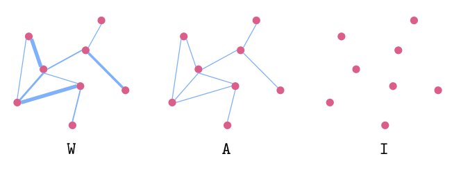
Figure 8: Varying levels of ECK.

Table 13: Single-step forecasting RMSE and MAE for different ECK levels.

	ECK	RMSE				MAE
		tennis	wikimath	pedalme	cpox	tennis	wikimath	pedalme	cpox
LightCTS	W	199.04	319.47	1.58	0.84	13.08	96.90	1.24	0.54
	A	195.47	323.00	1.54	0.85	11.92	96.13	1.19	0.53
	I	199.30	319.33	1.53	0.85	12.87	101.6	1.21	0.53
GRAM-ODE	W	206.50	484.90	0.99	0.98	22.94	265.65	0.68	0.63
	A	161.18	683.73	0.99	0.98	19.12	330.90	0.68	0.63
	I	161.18	821.57	0.99	0.98	19.11	403.45	0.68	0.63
STGODE	W	172.16	279.87	0.91	0.83	14.01	118.8	0.62	0.54
	A	165.92	272.84	0.91	0.84	13.30	107.4	0.61	0.53
	I	169.27	272.38	0.91	0.83	13.64	97.25	0.63	0.53
mspace-S$\mu$	A	105.32	563.69	0.86	1.58	6.26	113.27	0.71	1.20
	I	105.47	228.13	0.79	1.47	6.26	94.89	0.60	1.11

We make the following observations from the results of the experiment presented in Table 13:

• mspace-S$\mu$ achieves the best performance across all datasets, except for cpox, and does so without utilising any information from the graph structure (I). STGODE and LightCTS exhibit similar trend on wikimath and pedalme, respectively.

• For the tennis dataset, LightCTS and STGODE show their best performance when the graph is unweighted, which suggests that the graph structure information is useful.

• GRAM-ODE is the only model which exhibits ideal behaviour for wikimath dataset, i.e., the performance improves with increasing knowledge about the graph structure. However, the performance of GRAM-ODE remains the same for different ECK levels in pedalme and cpox.

It is essential to highlight that if an algorithm does not exhibit enhanced performance with a higher ECK level, it does not automatically imply that the edge configuration does not influence the evolution of node features. Moreover, it is crucial not to attribute a model’s shortcomings solely to its design, as the lack of correlation between edge weights and node features may genuinely exist in temporal graph datasets.

For GNN-based models, unweighted graph information is sufficient since the model can adapt and learn the necessary weights once the graph structure is known. For instance, in graph convolution networks (GCN), the convolution operation is expressed as $\tilde{{\bm{A}}}{\bm{X}}\bm{\Theta}$, with $\tilde{{\bm{A}}}$ being the normalized adjacency matrix, ${\bm{X}}$ the node feature matrix, and $\bm{\Theta}$ representing the weights learned during training (Rahman & Coon, 2024). Consider a scenario with a normalized adjacency matrix $\tilde{{\bm{A}}}$ from a weighted graph and $\tilde{{\bm{A}}}^{\prime}$ from its unweighted version. It can be argued that it is theoretically feasible to determine model weights $\bm{\Theta^{\prime}}$ such that $\tilde{{\bm{A}}}^{\prime}{\bm{X}}\bm{\Theta}^{\prime}\approx\tilde{{\bm{A}}}{\bm{X}}\bm{\Theta}$. However, in some cases, the model working on the unweighted graph might take more steps to achieve the same performance, and sometimes, it might get stuck in a local minimum.

Appendix F Additional Related Works

F.1 Recurrent Neural Network

We examine our model in the light of Recurrent Neural Networks (RNNs) (Chung et al., 2014). We consider $\{\bm{\varepsilon}_{t}:\forall t\in[T-1]\}$ to be the input and $\{\bm{\varepsilon}_{t+1}:\forall t\in[T]\}$ to be the corresponding output. We denote the hidden state at time step $t$ as ${\bm{s}}_{t}$. The RNN works through the following two equations:

$${\bm{s}}_{t}=f\left({\bm{U}}\bm{\varepsilon}_{t}+{\bm{V}}{\bm{s}}_{t-1}+{\bm{b}}\right),$$ (18)

$$\bm{\varepsilon}_{t+1}={\bm{W}}{\bm{s}}_{t}+{\bm{c}},$$ (19)

where $f(\cdot)$ is the activation function and $({\bm{U}},{\bm{V}},{\bm{W}},{\bm{b}},{\bm{c}})$ are the set of weights that are learnt during the training phase. We can draw a parallel with our method by setting ${\bm{U}}={\bm{I}},{\bm{V}}=\mathbf{0},{\bm{b}}=\mathbf{0}$, and $f\equiv\Psi$ giving us: ${\bm{h}}_{t}=\Psi(\bm{\varepsilon}_{t})$. However, for the next step we rely on a more general definition $\bm{\varepsilon}_{t+1}=\Omega({\bm{s}}_{t})$, which may or may not be a deterministic function of ${\bm{s}}_{t}$.

Now we compare our work with Variational RNN (VRNN) (Chung et al., 2015), whose operation can be described through the following two equations:

$${\bm{s}}_{t}=f_{\theta}(\bm{\varepsilon}_{t},{\bm{s}}_{t-1}),$$ (20)

$$\bm{\varepsilon}_{t+1}\sim p(\bm{\varepsilon}_{t+1}|\bm{\varepsilon}_{t},\bm{\varepsilon}_{t-1},\cdots)=g_{\tau}({\bm{s}}_{t}),$$ (21)

where $g_{\tau}({\bm{s}})$ is a distribution function parameterised by $\tau$ and $f_{\theta}(\cdot)$ denotes a neural network (NN) with parameter $\theta$.

Our model is similar to RNN, if the function $f_{\theta}$ does not take the previous state as an input, i.e., ${\bm{s}}_{t}=f_{\theta}(\bm{\varepsilon}_{t})$ is equivalent to ${\bm{s}}_{t}=\Psi(\bm{\varepsilon}_{t})$ which is simply the Markov assumption collapsing $\bm{\varepsilon}_{t+1}\sim p(\bm{\varepsilon}_{t+1}|\bm{\varepsilon}_{t},\bm{\varepsilon}_{t-1},\cdots)$ to $\bm{\varepsilon}_{t+1}\sim p(\bm{\varepsilon}_{t+1}|\bm{\varepsilon}_{t})$, or simply $\bm{\varepsilon}_{t+1}\sim p(\bm{\varepsilon}_{t+1}|{\bm{s}}_{t})$.

Another major point of difference that separates our model from any NN-based techniques is that we rely on maximum likelihood estimation to learn $\Omega({\bm{s}})$ while the NN techniques rely on learning the weights through gradient descent methods. Moreover, we write $\Omega({\bm{s}})$ as a sample of the probability distribution $p(\bm{\varepsilon}^{\prime}|{\bm{s}})$ instead of defining $\Omega({\bm{s}})$ as the probability distribution itself, as is the case with RNNs.

In Fig. 9, we compare our model’s architecture with the folded representation of an RNN.

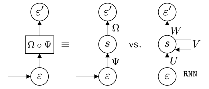
Figure 9: Comparison with RNN.

F.2 Gaussian Mixture Model

A Gaussian mixture model (GMM) (McLachlan et al., 2019) is a weighted sum of multiple Gaussian distribution components. An $M$-component GMM can be written as:

$$p({\bm{x}}|\bm{\lambda})=\sum_{i\in[M]}w_{i}\cdot{\mathcal{N}}({\bm{x}};\bm{\mu}_{i},\bm{\Sigma}_{i}),$$ (22)

where $\sum_{i\in[M]}w_{i}=1$ and $\bm{\lambda}=\{(w_{i},\bm{\mu}_{i},\bm{\Sigma}_{i}):\forall i\in[M]\}$.

We can express $p(\bm{\varepsilon}^{\prime}|{\bm{s}})$ as a GMM having $|{\mathcal{S}}|$ components:

$$p(\bm{\varepsilon}^{\prime}|{\bm{s}})=\sum_{{\bm{s}}^{\prime}\in{\mathcal{S}}}\mathbb{I}\{{\bm{s}}={\bm{s}}^{\prime}\}\cdot{\mathcal{N}}(\bm{\varepsilon}^{\prime};\bm{\mu}({\bm{s}}^{\prime}),\bm{\Sigma}({\bm{s}}^{\prime})),$$ (23)

where ${\mathcal{S}}$ is the range of $\Psi$, and $\sum_{{\bm{s}}^{\prime}\in{\mathcal{S}}}\mathbb{I}\{{\bm{s}}={\bm{s}}^{\prime}\}=1$ is satisfied which makes $p(\bm{\varepsilon}^{\prime}|{\bm{s}})$ a vaild GMM.

In a typical GMM, we need to learn $\bm{\lambda}=\{(w_{i},\bm{\mu}_{i},\bm{\Sigma}_{i}):\forall i\in[M]\}$ which is done through expectation-maximisation (EM) algorithm, or maximum a posteriori (MAP) estimation. However, to learn this simplified GMM, we need to estimate the values of $\{\bm{\mu}({\bm{s}}^{\prime}),\bm{\Sigma}({\bm{s}}^{\prime}):\forall{\bm{s}}^{\prime}\in{\mathcal{S}}\}$ which can be done simply through maximum likelihood estimation (MLE). We first define the set ${\mathcal{Z}}\triangleq\{\bm{\varepsilon}_{t+1}:\Psi(\bm{\varepsilon}_{t})={\bm{s}}^{\prime},\,\forall t\in[T^{\prime}]\}$. Then, we arrange the elements of ${\mathcal{Z}}$ as a matrix ${\bm{Z}}\in\mathbb{R}^{\dim{(\bm{\varepsilon})}\times T^{\prime}}$ and find the mean vector and covariance matrix of state ${\bm{s}}^{\prime}$ as follows:

$$\bm{\mu}({\bm{s}}^{\prime})=\frac{1}{T^{\prime}}{\bm{Z}}\,\bm{1}_{T^{\prime}\times 1},$$ (24)

$$\bm{\Sigma}({\bm{s}}^{\prime})=\frac{1}{T^{\prime}}\big{(}{\bm{Z}}-\bm{\mu}({\bm{s}}^{\prime})\big{)}\big{(}{\bm{Z}}-\bm{\mu}({\bm{s}}^{\prime})\big{)}^{\top}.$$ (25)

F.3 Opinion Dynamics

Opinion dynamics is the process by which a set of agents update their opinions based on interactions with each other, according to an underlying rule (Zha et al., 2021). The interaction of the agents can be modeled as a temporal graph with the node features as opinion vectors. In this context, opinion forecasting (De et al., 2016) refers to the problem of predicting the future opinions of the agents based on the historically observed opinions. It is clear that opinion forecasting is node regression applied to social networks.

References

- Bishop (2006) Bishop, C. M. Pattern recognition and machine learning. Information science and statistics. Springer, New York, 2006. ISBN 978-0-387-31073-2.
- Box & Pierce (1970) Box, G. E. P. and Pierce, D. A. Distribution of Residual Autocorrelations in Autoregressive-Integrated Moving Average Time Series Models. Journal of the American Statistical Association, 65(332):1509–1526, December 1970. ISSN 0162-1459. doi: 10.1080/01621459.1970.10481180.
- Chung et al. (2014) Chung, J., Gulcehre, C., Cho, K., and Bengio, Y. Empirical Evaluation of Gated Recurrent Neural Networks on Sequence Modeling, December 2014. URL http://arxiv.org/abs/1412.3555. arXiv:1412.3555 [cs].
- Chung et al. (2015) Chung, J., Kastner, K., Dinh, L., Goel, K., Courville, A. C., and Bengio, Y. A Recurrent Latent Variable Model for Sequential Data. In Advances in Neural Information Processing Systems, volume 28. Curran Associates, Inc., 2015. URL https://proceedings.neurips.cc/paper/2015/hash/b618c3210e934362ac261db280128c22-Abstract.html.
- De et al. (2016) De, A., Valera, I., Ganguly, N., Bhattacharya, S., and Rodriguez, M. G. Learning and Forecasting Opinion Dynamics in Social Networks. 2016.
- Fang et al. (2021) Fang, Z., Long, Q., Song, G., and Xie, K. Spatial-Temporal Graph ODE Networks for Traffic Flow Forecasting. In Proceedings of the 27th ACM SIGKDD Conference on Knowledge Discovery & Data Mining, pp. 364–373, August 2021. doi: 10.1145/3447548.3467430. URL http://arxiv.org/abs/2106.12931. arXiv:2106.12931 [cs].
- Harary & Norman (1960) Harary, F. and Norman, R. Z. Some properties of line digraphs. Rendiconti del Circolo Matematico di Palermo, 9(2):161–168, May 1960. ISSN 0009-725X, 1973-4409. doi: 10.1007/BF02854581. URL http://link.springer.com/10.1007/BF02854581.
- Kipf & Welling (2016) Kipf, T. N. and Welling, M. Variational Graph Auto-Encoders, November 2016. URL http://arxiv.org/abs/1611.07308. arXiv:1611.07308 [cs, stat].
- Kipf & Welling (2017) Kipf, T. N. and Welling, M. Semi-Supervised Classification with Graph Convolutional Networks, February 2017. URL http://arxiv.org/abs/1609.02907. arXiv:1609.02907 [cs, stat].
- Komodakis (2019) Komodakis, M. S. N. GraphVAE: Towards Generation of Small Graphs Using Variational Autoencoders. 2019.
- Lai et al. (2023) Lai, Z., Zhang, D., Li, H., Jensen, C. S., Lu, H., and Zhao, Y. LightCTS: A Lightweight Framework for Correlated Time Series Forecasting, February 2023. URL http://arxiv.org/abs/2302.11974. arXiv:2302.11974 [cs].
- Li et al. (2017) Li, Y., Yu, R., Shahabi, C., and Liu, Y. Diffusion convolutional recurrent neural network: Data-driven traffic forecasting. arXiv preprint arXiv:1707.01926, 2017.
- Liu et al. (2023) Liu, Z., Shojaee, P., and Reddy, C. K. Graph-based Multi-ODE Neural Networks for Spatio-Temporal Traffic Forecasting. arXiv preprint arXiv:2305.18687, 2023.
- Longa et al. (2023) Longa, A., Lachi, V., Santin, G., Bianchini, M., Lepri, B., Lio, P., Scarselli, F., and Passerini, A. Graph Neural Networks for temporal graphs: State of the art, open challenges, and opportunities. arXiv preprint arXiv:2302.01018, 2023.
- McLachlan et al. (2019) McLachlan, G. J., Lee, S. X., and Rathnayake, S. I. Finite Mixture Models. 2019.
- Micheli & Tortorella (2022) Micheli, A. and Tortorella, D. Discrete-time dynamic graph echo state networks. Neurocomputing, 496:85–95, 2022. Publisher: Elsevier.
- Murphy (2002) Murphy, K. P. Dynamic Bayesian Networks. November 2002.
- Pareja et al. (2020) Pareja, A., Domeniconi, G., Chen, J., Ma, T., Suzumura, T., Kanezashi, H., Kaler, T., Schardl, T., and Leiserson, C. Evolvegcn: Evolving graph convolutional networks for dynamic graphs. In Proceedings of the AAAI conference on artificial intelligence, volume 34, pp. 5363–5370, 2020. Issue: 04.
- Rahman & Coon (2024) Rahman, A. U. and Coon, J. P. A Primer on Temporal Graph Learning, January 2024. URL http://arxiv.org/abs/2401.03988. arXiv:2401.03988 [cs, eess].
- Rao et al. (2022) Rao, X., Wang, H., Zhang, L., Li, J., Shang, S., and Han, P. FOGS: First-Order Gradient Supervision with Learning-based Graph for Traffic Flow Forecasting. In Proceedings of the Thirty-First International Joint Conference on Artificial Intelligence, pp. 3926–3932, Vienna, Austria, July 2022. International Joint Conferences on Artificial Intelligence Organization. ISBN 978-1-956792-00-3. doi: 10.24963/ijcai.2022/545. URL https://www.ijcai.org/proceedings/2022/545.
- Shumway & Stoffer (2017) Shumway, R. H. and Stoffer, D. S. Time Series Analysis and Its Applications: With R Examples. Springer Texts in Statistics. Springer International Publishing, Cham, 2017. ISBN 978-3-319-52451-1 978-3-319-52452-8. doi: 10.1007/978-3-319-52452-8. URL http://link.springer.com/10.1007/978-3-319-52452-8.
- Veličković et al. (2018) Veličković, P., Cucurull, G., Casanova, A., Romero, A., Liò, P., and Bengio, Y. Graph Attention Networks, February 2018. URL http://arxiv.org/abs/1710.10903. arXiv:1710.10903 [cs, stat].
- Welch (1997) Welch, G. An Introduction to the Kalman Filter. 1997.
- Wu et al. (2019) Wu, Z., Pan, S., Long, G., Jiang, J., and Zhang, C. Graph WaveNet for Deep Spatial-Temporal Graph Modeling, May 2019. URL http://arxiv.org/abs/1906.00121. arXiv:1906.00121 [cs, stat].
- Wu et al. (2021) Wu, Z., Pan, S., Chen, F., Long, G., Zhang, C., and Yu, P. S. A Comprehensive Survey on Graph Neural Networks. IEEE Transactions on Neural Networks and Learning Systems, 32(1):4–24, January 2021. ISSN 2162-237X, 2162-2388. doi: 10.1109/TNNLS.2020.2978386. URL https://ieeexplore.ieee.org/document/9046288/.
- Zha et al. (2021) Zha, Q., Kou, G., Zhang, H., Liang, H., Chen, X., Li, C.-C., and Dong, Y. Opinion dynamics in finance and business: a literature review and research opportunities. Financial Innovation, 6(1):44, January 2021. ISSN 2199-4730. doi: 10.1186/s40854-020-00211-3. URL https://doi.org/10.1186/s40854-020-00211-3.
- Zhao et al. (2019) Zhao, L., Song, Y., Zhang, C., Liu, Y., Wang, P., Lin, T., Deng, M., and Li, H. T-gcn: A temporal graph convolutional network for traffic prediction. IEEE transactions on intelligent transportation systems, 21(9):3848–3858, 2019. Publisher: IEEE.