Analysis of Time-Evolution of Gaussian Wavepackets in Non-Hermitian Systems

Abstract

Simulation and analysis of multidimensional dynamics of a quantum non-Hmeritian system is a challenging problem. Gaussian wavepacket dynamics has proven to be an intuitive semiclassical approach to approximately solving the dynamics of quantum systems. A Gaussian wavepacket approach is proposed for a continuous space extension to the Hatano-Nelson model that enables transparent analysis of the dynamics in terms of complex classical trajectories. We demonstrate certain cases where the configuration space trajectory can be made fully real by transforming the initial conditions to account for the non-Hermiticity appropriately through the momentum coordinates. However, in general the complex phase space is unavoidable. For the cases where the trajectory is real, the effective force can be decomposed into that due to the potential energy surface and that due to the imaginary vector potential. The impact of the vector potential on the trajectory of the wavepacket is directly proportional to both the strength of the vector potential and the width of the wavepacket.

I Introduction

Quantum mechanics is built on the foundation of Hermitian operators. Hermiticity, especially of the Hamiltonian, guarantees a real spectrum, orthonormal eigenstates, and a unitary time evolution operator. However, open-quantum systems often incorporate interactions with the environment which involve gain and loss of energy and / or particles can no longer be modeled using Hermitian Hamiltonians. Such non-Hermitian systems have been under intense study over the past few decades [1, 2, 3, 4], with simulations of the dynamics in such systems becoming a focus in recent times [5, 6, 7, 8, 9, 10].

The wide-ranging applicability and interest of these non-Hermitian systems have been outlined in various review articles [11, 12, 13]. It is notable that despite Hermiticity being one of the corner-stones of quantum mechanics, over the past few decades, it has been shown that Hamiltonians that respect the parity-time ($\mathcal{PT}$) symmetry have real eigenvalues [2]. This observation has spawned research into $\mathcal{PT}$-symmetric quantum mechanics [3, 14, 4, 15, 16]. Optics in particular has proven to be an exceptionally versatile landscape for probing the effects of $\mathcal{PT}$-symmetry and non-Hermiticity [17, 18, 19, 20]. Rüter et al. [19] have observed both a spontaneous breaking of the $\mathcal{PT}$-symmetry as well as a violation of the left-right symmetry in some optical systems.

Li and Wan [8] have recently investigated the time evolution of a Gaussian wavepacket under a continuum extension of the Hatano-Nelson model [1] in a finite 1-dimensional box. In addition to the anomolous reflection from boundaries, that they have dubbed the “dynamical” skin effect, they have also noticed an acceleration being produced by the non-Hermitian term. These very interesting observations lead naturally to the question of how the non-Hermiticity in the system “interacts” with an external potential. How does the dynamics of a particle in a potential landscape change due to the non-Hermitian terms. Semiclassical analysis seems to be invaluable in analysing the dynamics of such complicated systems.

Various methods for simulating the dynamics of a quantum sytem in a semiclassical manner has been developed over the years. These are generally obtained by evaluating the Feynman path integral [21] under stationary phase approximation valid under under the limit of $\hbar\to 0$. This has spawned a wide range of approximations [22, 23, 24, 25, 26]. Gaussian wavepacket dynamics (GWD) [27, 28, 29] provides an alternate, complementary approach to semiclassical simulations where one tracks the evolution of a Gaussian wavepacket over time and realizes that under certain conditions the center of the wave packet and the average momentum follow the classical equations of motion. Recently, GWD, with further approximations, has been applied to ab initio systems [30, 31, 32, 33]. The original GWD has also been extended to classical Hamiltonians over a complex phase space to handle classically forbidden processes [34, 35]. This complex version of GWD called the generalized Gaussian wavepacket dynamics (GGWD) is closely related to path integrals in coherent state representation [36].

In this work we present the thawed Gaussian dynamics corresponding to a generalized Hatano-Nelson (HN) continuum model under an external potential. The non-Hermitian term appears as an imaginary vector potential. Despite the initial average position and momentum corresponding to a Gaussian wavepacket being real, the imaginary vector potential ensures that the classical trajectory goes over a complex phase space. Thus, in general, the method requires complex phase space classical trajectories and corresponding generalized Gaussians. However, we show that it is possible to use the properties of these general Gaussians to transform the initial momentum into the complex plane dictated by the imaginary vector potential, which ensures that the initial position and velocity are real. Consequently, the corresponding configuration space trajectory, which is called the “guiding” trajectory, becomes completely real and identical to the classical trajectory in absence of the non-Hermitian term. The real phase space center of the wavepacket is obtained as a transformation of this real guiding trajectory. We also show that the deviation of the real center of the wavepacket from the guiding trajectory is related to the width of the wavepacket, which in turn depends on the non-Hermitian terms.

While the results present here are exact for quadratic external potentials and linear imaginary vector potential, higher order potentials are dealt with at a local harmonic level. The paper is organized as follows: Sec. II outlines the model and develops the non-Hermitian thawed Gaussian wavepacket dynamics (NH-GWD) approach. Numerical demonstrations of the method are provided in Sec. III. Finally, some concluding remarks and future directions are provided in Sec. IV.

II Model & Non-Hermitian Thawed Gaussian Wavepacket Dynamics

Consider a generalized HN-inspired continuum model given by [1]:

$$H =\sum_{j}\frac{1}{2m_{j}}\left(P_{j}+ib_{j}(X_{j})\right)^{2}+V(\mathbf{X})$$ (1)

$$=\sum_{j}\left(-\frac{\hbar^{2}}{2m_{j}}\partial_{j}^{2}+\frac{\hbar b_{j}(x_{j})}{m_{j}}\partial_{j}+\frac{\hbar}{2m_{j}}b^{\prime}_{j}(x_{j})-\frac{b_{j}^{2}(x_{j})}{2m_{j}}\right)$$

$$+V(\mathbf{x})$$ (2)

where $X_{j},P_{j}$ are the position and momentum operators along the $j$th dimension, $b_{j}$ is a real function that brings in the non-Hermiticity, and $\partial_{j}=\partialderivative{x_{j}}$. The non-Hermitian part, brought in by the $b$ functions, can be interpreted as an imaginary vector potential. Discretizing Eq. 2 on a lattice reveals that $b_{j}$ causes the left-hopping amplitude and the right-hopping amplitude along the $j$th dimension to be different making the system non-Hermitian.

We want to understand the dynamics of a generalized Gaussian wavepacket. We assume that the propagated wavepacket retains its Gaussian form given by [35]

$$\innerproduct{\mathbf{x}}{\alpha,\mathbf{q},\mathbf{p},\gamma,t} =\exp\left(\frac{i}{\hbar}\left(\sum_{ij}\alpha_{ij}(t)(x_{i}-q_{i}(t))(x_{j}-q_{j}(t))\right.\right.$$

$$\left.\left.+\sum_{j}p_{j}(t)(x_{j}-q_{j}(t))+\gamma(t)\right)\right)$$ (3)

where the time-dependent parameters, $\alpha_{ij}(t)$, $q_{j}(t)$, $p_{j}(t)$, and $\gamma(t)$ are in general all complex. The imaginary part of $\alpha_{ij}$ is related to the width of the wavepacket ($\sigma=\sqrt{\frac{\hbar}{2\imaginary\alpha}}$). If $q_{j}(t)$ and $p_{j}(t)$ are real, they represent the centre of the wavepacket and the momentum respectively. The term $\gamma(t)$ represents the time-dependent phase of the wave packet. Every generalized Gaussian wavepackets does not uniquely represent one wave function. Two wavepackets are the same if the following two quantities are the same for both of them:

$$-2\sum_{j}\alpha_{ij}(t)q_{j}(t)+p_{i}(t) =\text{const},$$ (4)

$$\gamma(t)+\sum_{ij}\alpha_{ij}(t)q_{i}(t)q_{j}(t)-\sum_{j}p_{j}(t)q_{j}(t) =\text{const}.$$ (5)

The position and momentum parameters in a generalized Gaussian wavepacket do not correspond directly to the physically relevant phase space location of the wavepacket, which are real quantities. By considering the real and imaginary parts of Eq. 4, conversion from the complex phase space to the real phase space is enabled by [34]

$$\mathbf{Q}(t) =\real\mathbf{q}(t)+(\imaginary\alpha(t))^{-1}\left(\real\alpha(t)\imaginary\mathbf{q}(t)-\frac{1}{2}\imaginary\mathbf{p}(t)\right)$$ (6)

$$\mathbf{P}(t) =\real\mathbf{p}(t)+2\imaginary\alpha(t)\imaginary\mathbf{q}(t)+2\real\alpha(t)\left(\mathbf{Q}(t)-\mathbf{q}(t)\right)$$ (7)

There are several restrictions to GWD: first, it is exact for upto quadratic potentials; second, it cannot in general account for classically forbidden processes; and third, if the initial state is a superposition of Gaussians, the norm is not necessarily conserved. The non-uniqueness of the generalized Gaussian wavepackets can be leveraged to overcome these restrictions by choosing a complex phase space initial condition taylored to the final state [34, 35].

GWD assumes that the potential can treated under a local harmonic approximation:

$$V(\mathbf{x}) =V(\mathbf{q})+V^{(1)}(\mathbf{q})\cdot(\mathbf{x}-\mathbf{q})$$

$$+(\mathbf{x}-\mathbf{q})\cdot V^{(2)}(\mathbf{q})\cdot(\mathbf{x}-\mathbf{q})$$ (8)

which works if the potential is relatively slowly varying over the width of the wavepacket. Because $b_{j}^{2}$ contributes to an effective potential, for this work we assume a locally linear imaginary potential,

$$b_{j}(x_{j}) =b_{j}(q_{j})+b_{j}^{(1)}(q_{j})(x_{j}-q_{j}),$$ (9)

which makes $b_{j}^{2}$ a locally quadratic function.

Solving the time-dependent Schrödinger equation,

$$i\hbar\derivative{\ket{\alpha,\mathbf{q},\mathbf{p},\gamma,t}}{t} =H\ket{\alpha,\mathbf{q},\mathbf{p},\gamma,t},$$ (10)

we get equations of motion (EOM) for $\alpha$, $\mathbf{q}$, and $\mathbf{p}$

$$\sum_{l}2\alpha_{jl}\dot{q}_{l}(t)-\dot{p}_{j}(t) =V^{(1)}_{j}(\mathbf{q}(t))-\frac{b_{j}(q_{j}(t))b_{j}^{(1)}(q_{j}(t))}{m_{j}}+\sum_{k}\frac{2\alpha_{jk}(t)}{m_{k}}(p_{k}(t)+ib_{k}(q_{k}(t)))+\frac{ip_{j}(t)b_{j}^{(1)}(q_{j})}{m_{j}}$$ (11)

$$-\dot{\alpha}_{kl} =V^{(2)}_{kl}(\mathbf{q}(t))-\frac{b_{k}^{(1)2}(q(t))}{2m_{k}}\delta_{kl}+2i\frac{\alpha_{kl}(t)b_{l}^{(1)}(q_{l})}{m_{l}}+2\sum_{j}\frac{\alpha_{kj}(t)\alpha_{jl}(t)}{m_{j}}$$ (12)

$$\sum_{j}p_{j}(t)\dot{q}_{j}(t)-\dot{\gamma}(t) =V(\mathbf{q}(t))+\sum_{j}\left(\hbar\frac{b^{(1)}_{j}(q_{j}(t))}{m_{j}}-\frac{b_{j}^{2}(q_{j}(t))}{2m_{j}}+\frac{ip_{j}(t)b_{j}(q_{j}(t))}{m_{j}}+\frac{p_{j}^{2}(t)-2i\hbar\alpha_{jj}(t)}{2m_{j}}\right)$$ (13)

Consider the classical equations of motion under the Hamiltonian Eq. 2,

$$\dot{q}_{j}(t) =\frac{p_{j}+ib_{j}(q_{j})}{m_{j}}$$ (14)

$$\dot{p}_{j}(t) =-\partial_{j}V(\mathbf{q})-\frac{ib_{j}^{(1)}(q_{j})}{m_{j}}\left(p_{j}+ib_{j}(q_{j})\right).$$ (15)

These classical equations satisfy Eq. 11. However, notice that the imaginary vector potential makes the classical trajectory, $(\mathbf{q}(t),\mathbf{p}(t))$, are in general complex, even if the initial conditions, $(\mathbf{q}(0),\mathbf{p}(0))$, are real. Using Eq. 14, we can simplify Eq. 13 to

$$\dot{\gamma}(t) =\sum_{j}\frac{p_{j}^{2}(t)}{2m_{j}}-V(\mathbf{q}(t))+i\hbar\sum_{j}\frac{\alpha_{jj}(t)}{m_{j}}$$

$$+\sum_{j}\frac{b_{j}^{2}(q_{j}(t))-2\hbar b^{(1)}_{j}(q_{j}(t))}{2m_{j}}$$ (16)

So we now have the full EOM for the Gaussian wavepacket given by Eqs. 12, and 14 – 16. Notice that from Eqs. 14 and 15, though the initial position and momenta start off being real, the equations of motion make them complex. We will now show that for the cases of a constant and a linear imaginary vector potential, it is possible to transform the initial conditions in such a manner that the trajectory becomes real in configuration space. This “guiding” trajectory will allow us to decompose the effects of the external potential from that of the non-Hermitian terms in an intuitive manner.

II.1 Constant imaginary vector potential

Suppose $b_{j}(q_{j})=k_{j}$ is a constant. This is the case that has been recently studied by Li and Wan [8] with $V=0$. For the generalized Gaussian wavepacket, the EOM become:

$$\dot{q}_{j}(t) =\frac{p_{j}+ik_{j}}{m_{j}}$$ (17)

$$\dot{p}_{j}(t) =-\partial_{j}V(\mathbf{q})$$ (18)

$$-\dot{\alpha}_{kl} =V^{(2)}_{kl}(\mathbf{q}(t))+2\sum_{j}\frac{\alpha_{kj}(t)\alpha_{jl}(t)}{m_{j}}$$ (19)

$$\dot{\gamma}(t) =\sum_{j}\frac{p_{j}^{2}(t)}{2m_{j}}-V(\mathbf{q}(t))+i\hbar\sum_{j}\frac{\alpha_{jj}(t)}{m_{j}}+\sum_{j}\frac{k_{j}^{2}}{2m_{j}}$$ (20)

Generally, $\mathbf{q}(0)$ and $\mathbf{p}(0)$ are both real. Consequently using Eq. 17, we find that the initial velocity is complex. This of course leads to classical trajectories that are complex in both position and momentum dimensions. This problem can solved by analytically continuing the potential to a complex plane [34]. For the typical wavepacket, the initial value of $\alpha$ is usually imaginary ($\alpha(0)=\frac{i\hbar}{2\sigma^{2}}$).

However, let us see if we can construct real trajectories in some way. Notice at this stage that, if we arbitrarily choose a new, in general complex, initial momentum $\mathbf{\tilde{p}}(0)$, the physics would remain the same if, using Eq. 4, a corresponding new position is chosen as follows:

$$\mathbf{\tilde{q}}(0) =\mathbf{q}(0)+\frac{1}{2}\alpha(0)^{-1}\left(\mathbf{\tilde{p}}(0)-\mathbf{p}(0)\right),$$ (21)

and $\gamma(0)$ is changed according to Eq. 5. If $\mathbf{q}(0)$ is real, $\mathbf{\tilde{q}}(0)$ is real if $\mathbf{\tilde{p}}(0)-\mathbf{p}(0)$ is imaginary because $\alpha(0)$ is initially imaginary. Additionally,

$$\mathbf{\dot{\tilde{q}}}(0) =m^{-1}\left(\mathbf{\tilde{p}}(0)+i\mathbf{k}\right).$$ (22)

Now, if we set $\mathbf{\tilde{p}}(0)=\mathbf{p}(0)-i\mathbf{k}$, then both $\mathbf{\tilde{q}}(0)=\mathbf{q}(0)-\frac{i}{2}(\alpha(0))^{-1}\mathbf{k}$ and $\mathbf{\dot{\tilde{q}}}(0)=m^{-1}\mathbf{p}(0)$ both become real. With such a transformation of the initial positions and momenta into a generalized Gaussian wavepacket, the usual classical equations of motion,

$$m\mathbf{\ddot{\tilde{q}}} =-\partial_{j}V(\mathbf{\tilde{q}}),$$ (23)

$$\mathbf{\tilde{p}}(t) =m\mathbf{\dot{\tilde{q}}}(t)-i\mathbf{k}$$ (24)

give real positions and velocities with no impact from the imaginary vector potential $i\mathbf{k}$. This trajectory, $\mathbf{\tilde{q}}(t)$ which is uniquely determined only via the external potential, is the “guiding” classical trajectory. However, the corresponding momenta are complex. Converting back to real phase space coordinates using Eqs. 6 and 7, one obtains,

$$\mathbf{Q}(t) =\mathbf{\tilde{q}}(t)+\frac{1}{2}(\imaginary\alpha(t))^{-1}\mathbf{k}$$ (25)

$$\mathbf{P}(t) =m\mathbf{\dot{\tilde{q}}}(t)+\real\alpha(t)(\imaginary\alpha(t))^{-1}\mathbf{k}$$ (26)

With this, we have solved the problem for a constant imaginary vector potential. This solution is exact for systems upto a quadratic potential. Beyond that this effectively treats the potential under a local harmonic approximation. While the full generalized Gaussian wavepacket analysis of these systems following Huber and Heller [34] will be done in a future work, the current development already gives us different perspectives to analyse the problem from.

Notice that the classical equations of motion, Eq. 23 for the guiding trajectory, knows nothing about $\mathbf{k}$, it follows the forces from the potential energy landscape.The equation of motion of $\alpha(t)$, Eq. 29, is independent of $\mathbf{k}$, which in this case is zero. So, $\alpha(t)$ only depends on the external potential and the guiding trajectory. It also knows nothing about the non-Hermitian term. The imaginary vector potential enters the trajectory in Eq. 25, when we insist upon a fully real phasespace. The prefactor of $(\imaginary\alpha(t))^{-1}$ is proportional to the dynamical width of the wavepacket $\sigma(t)$. Thus the impact of $\mathbf{k}$ increases as the wavepacket gets broader.

Now, let us obtain the analytical solution of some known cases.

II.1.1 1D Free Particle

Let us obtain the analytic results for some of the simple cases. First consider a free particle in one dimension, $V(q)=0$ as explored in Ref. [8], the solution is [27]:

$$\tilde{q}(t) =\tilde{q}(0)+p(0)t/m$$ (27)

$$\alpha(t) =\frac{m\alpha(0)}{2\alpha(0)t+m}=\frac{im\hbar}{2i\hbar t+2m\sigma^{2}(0)},$$ (28)

$$=\frac{m\hbar^{2}t}{2m^{2}\sigma^{4}(0)+2\hbar^{2}t^{2}}+\frac{im^{2}\hbar\sigma^{2}(0)}{2m^{2}\sigma^{4}(0)+2\hbar^{2}t^{2}}$$ (29)

where $\sigma(0)$ is the initial standard deviation of the wavepacket. Consequently,

$$Q(t) =q(0)+\frac{p(0)}{m}t+\frac{\hbar k}{m^{2}\sigma^{2}(0)}t^{2}$$ (30)

$$P(t) =p(0)+\frac{\hbar k}{m\sigma^{2}(0)}t$$ (31)

Notice that the only acceleration term comes because of the imaginary potential $k$ that acts like a constant external force.

So, it is natural to be curious if this force can be “counteracted,” if we have a linear external potential leading to a constant force.

II.1.2 1D Linear Ramp

Consider the case where $V(x)=\beta x$. For this case, we will have:

$$p(t) =p(0)-\beta t$$ (32)

$$\tilde{q}(t) =\tilde{q}(0)+\frac{p(0)}{m}t-\frac{\beta}{2m}t^{2}.$$ (33)

Since the potential is linear, the solution for $\alpha(t)$ remains the same as in Eq. 29. Therefore, the real phase space location of the wave packet will be given by:

$$Q(t) =\tilde{q}(t)+\left(\frac{\sigma^{2}(0)}{\hbar}+\frac{\hbar t^{2}}{m^{2}\sigma^{2}(0)}\right)k$$ (34)

$$=q(0)+\frac{p(0)}{m}t+\left(\frac{\hbar k}{m^{2}\sigma^{2}(0)}-\frac{\beta}{2m}\right)t^{2}.$$ (35)

Therefore, if we choose $\beta=\frac{2\hbar k}{m\sigma^{2}(0)}$, the wavepackets center would behave as a free particle. We need to be careful at this stage. The “additive” nature of the forces due to the constant imaginary vector potential and the external potential field holds in this case because $\alpha(t)$ is not affected by the potential. For quadratic and higher potentials where $\alpha(t)$ itself would change, this feature will not appear.

II.1.3 1D Harmonic Oscillator

Next, we obtain the solutions for a harmonic $V(x)=\frac{1}{2}m\omega^{2}x^{2}$. It is well known that GWD is exact for these cases with the solution being given by [27]:

$$\tilde{q}(t) =\tilde{q}(0)\cos(\omega t)+\frac{p(0)}{m\omega}\sin(\omega t)$$ (36)

$$\alpha(t) =-\frac{m\omega}{2}\left(\frac{\frac{1}{2}m\omega-\alpha(0)\cot(\omega t)}{\alpha(0)+\frac{1}{2}m\omega\cot(\omega t)}\right)$$ (37)

$$=-\frac{m\omega}{2}\left(\frac{m^{2}\omega^{2}\sigma^{4}(0)-\hbar^{2}}{\hbar^{2}\tan^{2}(\omega t)+m^{2}\omega^{2}\sigma^{4}(0)\cot(\omega t)}\right.$$

$$\left.-i\frac{\hbar m\omega\sigma^{2}(0)}{\hbar^{2}\sin^{2}(\omega t)+m^{2}\omega^{2}\sigma^{4}(0)\cos^{2}(\omega t)}\right)$$ (38)

Therefore, the center of the wavepacket goes as

$$Q(t) =\tilde{q}(t)+\left(\frac{\hbar^{2}\sin^{2}(\omega t)+m^{2}\omega^{2}\sigma^{4}(0)\cos^{2}(\omega t)}{\hbar m^{2}\omega^{2}\sigma^{2}(0)}\right)k.$$ (39)

Notice that $\tilde{q}(t)$ is the guiding classical trajectory that already has the free harmonic oscillations with frequency $\omega$. The imaginary vector potential brings in an extra component of frequency $2\omega$ in the form of terms with $\sin^{2}(\omega t)$ and $\cos^{2}(\omega t)$.

II.2 Linear imaginary vector potential

We have shown that for a constant imaginary vector potential, it is possible to transform the initial condition to obtain trajectories that a completely real in the configuration space. Can a similar transformation be done for the case when $\mathbf{b}(\mathbf{q})=k\mathbf{q}+\mathbf{c}$?

Consider a wavepacket with initial phase space positions $\mathbf{q}(0)$ and $\mathbf{p}(0)$. While these are real, the problem is once again, that the trajectory would be come complex because of the imaginary vector potential, which renders $\dot{\mathbf{q}}(0)$ complex. Let us suppose that $\tilde{\mathbf{p}}(0)$ is the momentum that allows both the position and velocity to be real. Let the corresponding position be $\tilde{\mathbf{q}}(0)$. As in the previous section,

$$\tilde{\mathbf{q}}(0) =\mathbf{q}(0)+\frac{1}{2}\alpha(0)^{-1}\left(\tilde{\mathbf{p}}(0)-\mathbf{p}(0)\right)$$ (40)

$$\mathbf{\dot{\tilde{q}}}(0) =m^{-1}\left(\mathbf{\tilde{p}}(0)+i\mathbf{b}(\mathbf{\tilde{q}}(0))\right)$$ (41)

For $\tilde{\mathbf{q}}(0)$ to be real, $\mathbf{\tilde{p}}(0)-\mathbf{p}(0)$ has to be imaginary. Let $\mathbf{\tilde{p}}(0)=\mathbf{p}(0)+i\mathbf{f}$, where $i\mathbf{f}=2\alpha(0)(\mathbf{\tilde{q}}(0)-\mathbf{q}(0))$. This leads to

$$\mathbf{\dot{\tilde{q}}}(0) =m^{-1}\left(\mathbf{p}(0)+2\alpha(0)(\mathbf{\tilde{q}}(0)-\mathbf{q}(0))+i\mathbf{b}(\mathbf{\tilde{q}}(0))\right)$$ (42)

Given that $\alpha(0)$ is imaginary, $\mathbf{\dot{\tilde{q}}}(0)$ can be real only if the sum of the second and third terms is zero. This condition is equivalent to the following:

$$\mathbf{\tilde{q}}(0) =(2\imaginary\alpha(0)+k)^{-1}(2\imaginary\alpha(0)\mathbf{q}(0)-\mathbf{c})$$ (43)

$$i\mathbf{f} =-2\alpha(0)(2\imaginary\alpha(0)+k)^{-1}\mathbf{b}(\mathbf{q}(0))$$ (44)

With these initial conditions, the guiding classical trajectory has all real positions. Once again the imaginary part of the canonical is given by the imaginary vector potential evaluated at the guiding trajectory. The real phase space center of the wavepacket can be once again evaluated by Eqs. 6 and 7. The EOMs for $\alpha(t)$ and $\gamma(t)$ involve $\mathbf{b}(\mathbf{q})$ explicitly.

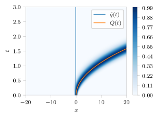
(a) $q(0)=0.0,p(0)=0.0$.

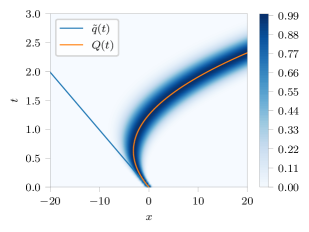
(b) $q(0)=0.0,p(0)=-10.0$.

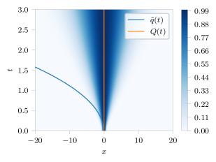
(c) $q(0)=0.0,p(0)=0.0$.

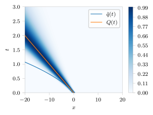
(d) $q(0)=0.0,p(0)=-10.0$.

Figure 1: Plot of $\absolutevalue{\psi(t,x)}^{2}$ as a function of position and time normalized to a maximum value of 1. The value of the imaginary potential $k=1$ and $m=1$. Top row: free particle; Bottom row: linear ramp with $\beta=\frac{2\hbar k}{m\sigma^{2}(0)}$.

III Results

First, we consider the case of a constant imaginary vector potential. In all these cases, we consider a wavepacket with $\alpha(0)=4i$. In Fig. 1, we show the dynamics of a wavepacket localized originally at $q(0)=0.0$ with different initial momenta under the non-Hermitian term, $k$, and a variable external potential. For the case of the free particle, Fig. 1 (a) and (b), our results match the analytic solutions in Ref. [8]. For the linear ramp, we have picked $\beta$ to be at the critical value of $\frac{2\hbar k}{m\sigma^{2}(0)}$. As a consequence, notice that in Fig. 1 (c) and (d) we only see the center, $Q(t)$, moving “unforced” in a straight line.

The magnitude of the wave function corresponding to the particle with no external potential and the linear ramp are shown in Fig. 2. While for the free particle, the norm increases, for the system in an external linear potential, the norm drops to zero. As is observed, the evolution of the magnitude of the wavefunction depends upon an interaction of the external potential and the imaginary vector potential.

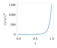
(a) $q(0)=0.0,p(0)=0.0$.

(b) $q(0)=0.0,p(0)=-10.0$.

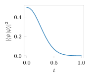
(c) $q(0)=0.0,p(0)=0.0$.

(d) $q(0)=0.0,p(0)=-10.0$.

Figure 2: Plot of $\absolutevalue{\innerproduct{\psi}{\psi}}^{2}$. Subfigures correspond to Fig. 1.

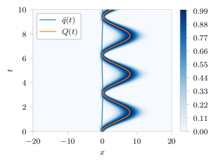
(a) $q(0)=0.0,p(0)=0.0$.

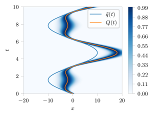
(b) $q(0)=0.0,p(0)=-10.0$.

Figure 3: Plot of $\absolutevalue{\psi(t,x)}^{2}$ as a function of position and time normalized to a maximum value of 1 for a wave packet moving under an external harmonic potential with $\omega=1$.

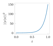
(a) $q(0)=0.0,p(0)=0.0$.

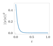
(b) $q(0)=0.0,p(0)=-10.0$.

Figure 4: Plot of norm of the wavepacket as it propagates through the external harmonic potential.

The dynamics gets interesting when we consider the particle in an external harmonic potential. The wavepacket is shown in Fig. 3. Notice that while in the case where the initial condition has 0 momentum and starts at the origin (Fig. 3 (a)), the dynamics has a single frequency, the one with a negative momentum (Fig. 3 (b)) shows an extra “bow”-like feature that is phase shifted with respect to the main oscillations. As a result of an interaction between the constant vector potential and the external harmonic potential, the dynamics seems to change between the two cases with different momenta.

The magnitude of the wavepacket for these two cases is shown in Fig. 4. Notice the periodicity of the norm for the case where the particle was initially stationary. In comparison, no such periodicity is seen in the case of the particle with $p(0)=-10.0$ within the time period of $t=10$.

(a) $q(0)=0.0,p(0)=0.0$.

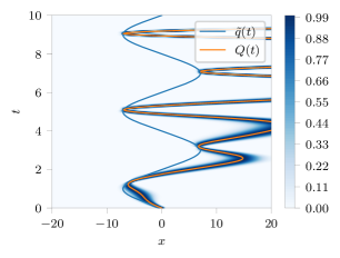
(b) $q(0)=0.0,p(0)=-10.0$.

Figure 5: Plot of $\absolutevalue{\psi(t,x)}^{2}$ as a function of position and time normalized to a maximum value of 1 for a wave packet moving under an external potential with $V(x)=\frac{1}{2}x^{2}+0.01x^{4}$.

Till now we have considered the dynamics under potentials that are quadratic or lower in power. In these cases, GWD is known to be exact. Let us consider $V(x)=\frac{1}{2}x^{2}+0.01x^{4}$. The dynamics for this anharmonic potential is shown for the same initial conditions in Fig. 5 simulated using a local harmonic approximation. As the anharmonicity gets stronger the dynamics would get increasingly approximate. One can significantly improve the quality of the simulation by using the generalized Gaussian wavepacket method.

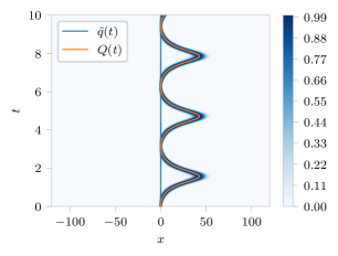
(a) $q(0)=0.0,p(0)=0.0$.

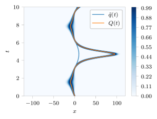
(b) $q(0)=0.0,p(0)=-10.0$.

Figure 6: Plot of $\absolutevalue{\psi(t,x)}^{2}$ as a function of position and time normalized to a maximum value of 1 for a wave packet moving under an external harmonic potential with $\omega=1$. The imaginary vector potential is $b(x)=0.1x+1.0$.

Next, consider a case with a linear imaginary vector potential $b(x)=0.1x+1.0$. We want to understand the interaction of this linear $b$ with an external harmonic potential $V(x)=\frac{1}{2}x^{2}$. Figure 6 shows the evolution of the wavepacket in this case. Notice the profound differences brought in by the change of the imaginary vector potential.

Finally, recent work has shown the existence of dynamical skin effect [8], where the reflection of a wavepacket from a hard boundary does not conserve the momentum. One of the difficulties in trying to study this using GWD is the problem of the hard boundary. A hard boundary can be simulated using a polynomial bounding potential of a high degree such as $V(x)=(x/L)^{2d}$ where $2L$ is the length of the box and $d$ is a sufficiently large number. GWD can only approximately account for the penetration of the quantum wave packet into classically forbidden regions if the potential is anharmonic. Therefore, the presence of the hard wall makes the simulations more inaccurate. Ideas from the general Gaussian wavepacket dynamics (GGWD) method [34, 35] will be leveraged in the future to make the simulations more accurate.

IV Conclusion

We have used Heller’s thawed Gaussian wavepacket dynamics [27, 28] to analyse the dynamics of non-Hermitian continuum quantum systems. While recent numerical studies have described curious features of the dynamics [8], a semiclassical analysis provides a general intuitive framework for thinking about these systems, and makes the connections to classical mechanics more obvious. As a problem of interest, we have chosen a generalized continuum Hatano-Nelson model in an external potential, with a potentially position-dependent non-Hermitian term. The non-Hermitian term appears as an imaginary vector potential.

We show that in general, due to the presence of the imaginary vector potential, the dynamics requires the use of complex phase space for specifying the time-evolving Gaussian wavepacket. However, using the non-uniqueness of these generalized Gaussian wavepackets, one can transform the initial condition in such a manner that the entire classical trajectory has real positions, obtained from the standard Newtonian equations of motion involving only the external potential. This “guiding” classical trajectory however has complex momenta. We show that the Newtonian equation of motion is independent of the vector potential, which affects the dynamics in three ways. The first way, which affects the guiding trajectory, is that the transformed initial condition is dependent on the imaginary vector potential. Second, the equations of motion for $\alpha(t)$ and $\gamma(t)$ are dependent on the vector potential. The third way by which the non-Hermitian term affects the dynamics is that on transforming back to fully real phase space coordinates, we notice that the center of the wavepacket deviates from the guiding trajectory by an amount that is proportional to the strength of the vector field at that point. The proportionality constant is the instantaneous width of Gaussian wavepacket. Thus, we have shown that the sharper the wavepacket and the weaker the non-Hermitian term, the closer the center is to the position of the guiding trajectory. It is interesting that the non-Hermitian term enters the dynamics by modifying $\alpha(t)$ and also through the instantaneous width of the wavepacket.

The interaction between the external potential and the non-Hermitian term becomes manifestly clear through this decomposition of the real phase space trajectory in terms of the guiding trajectory. We show that for a constant vector potential, the analysis becomes even more transparent, since $\alpha(t)$ becomes only dependent on the external potential. Then the spread remains exactly the same as that of the corresponding Hermitian system. The center of the wavepacket deviates by the width of the wavepacket times the non-Hermitian term.

The GWD approach provides a novel way of conceptualizing the dynamics under non-Hermitian systems. The decomposition in terms of the guiding classical trajectory and the deviations therefrom gives a classical picture to the dynamics. The GWD described in this work also provides the basis for future work that uses generalized Gaussian wavepackets for improved propagation [34, 35]. Additionally, trying to understand the dynamics of Gaussian wave packets in paradigmatic examples of $\mathcal{PT}$-symmetric non-Hermitian Hamiltonians would further develop our fundamental understanding of these interesting systems.