Bayesian scalar-on-network regression with applications to brain functional connectivity

Abstract

This study presents a Bayesian regression framework to model the relationship between scalar outcomes and brain functional connectivity represented as symmetric positive definite (SPD) matrices. Unlike many proposals that simply vectorize the connectivity predictors thereby ignoring their matrix structures, our method respects the Riemannian geometry of SPD matrices by modelling them in a tangent space. We perform dimension reduction in the tangent space, relating the resulting low-dimensional representations with the responses. The dimension reduction matrix is learnt in a supervised manner with a sparsity-inducing prior imposed on a Stiefel manifold to prevent overfitting. Our method yields a parsimonious regression model that allows uncertainty quantification of the estimates and identification of key brain regions that predict the outcomes. We demonstrate the performance of our approach in simulation settings and through a case study to predict Picture Vocabulary scores using data from the Human Connectome Project.

Keywords Neuroimaging  $\cdot$ Regression  $\cdot$ Brain connectivity  $\cdot$ Tangent space  $\cdot$ Riemannian geometry

1 Introduction

Neuroimaging techniques allow us to gain valuable insights into the activities of the brain by examining the functional connectivity, which measures the interrelationships among spatially distributed brain regions of interest (ROIs). Typically, functional connectivity can be estimated from functional magnetic resonance imaging (fMRI) data that capture the blood oxygen-level dependent (BOLD) signals over time (Bastos and Schoffelen, 2016). Advances in neuroimaging techniques and increased accessibility of data have led to a growing interest in studying the relationships of functional connectivity and cognitive or behaviour outcomes. For example, functional connectivity has been linked to intelligence (Song et al., 2008; He et al., 2020), language ability (Zhang et al., 2014; Tomasi and Volkow, 2020), cognitive impairment (Meskaldji et al., 2016; Lin et al., 2018), and neuropsychiatric disorders (Craddock et al., 2009; Venkataraman et al., 2012; Fair et al., 2013). The focus of our study is to build a regression model based on connectivity features that can be used to make predictions of various outcomes of interest while identifying key brain regions that contribute to the predictions.

A convenient approach for estimating individual functional connectivity is to compute sample covariances or correlations of the fMRI time series between ROIs (Dadi et al., 2019; Pervaiz et al., 2020; Strain et al., 2022). Alternative connectivity representations, including partial correlations (Ryali et al., 2012; Weaver et al., 2023) and graph-based statistics (Bullmore and Sporns, 2009; Vogelstein et al., 2012), have also been explored. Yet, they require the computation of matrix inversions or selection of representative summary statistics. Thus, our proposal focuses on correlation/covariance-based connectivity estimates that belong to the class of symmetric positive definite (SPD) matrices.

Given the estimated functional connectivity matrices, a common approach to build a regression model inputs vectorized matrices into conventional regression algorithms. This approach disregards the matrix nature of the features and produces an exceedingly large number of predictors that require substantial regularization or pre-screening of the features by performing massive univariate tests (Craddock et al., 2009; Zeng et al., 2012; Ming and Kundu, 2022). The resulting estimates can be difficult to interpret due to the lack of structure in the selected features. Another modelling approach adopts a two-stage procedure: first applying unsupervised methods to obtain a low dimension representation of connectivity matrices, then fitting a regression model with the low-dimensional features (Du et al., 2018; Zhang et al., 2019; Ma et al., 2022). However, representations learned in an unsupervised way to minimize the reconstruction error of the connectivity matrices may not necessarily yield features that are highly predictive of the response.

Within the frequentist paradigm, a variety of methods have been proposed for regression directly with matrix-valued predictors. While some methods specifically model symmetric matrices that naturally represent connectivity networks, other techniques deal with generic matrices or higher-order tensors (e.g. Zhou et al. (2013)), including symmetric matrices as a special case. Let the functional connectivity for the $i$-th subject be denoted as $\mathbf{M}_{i}\in\mathbb{R}^{p\times p}$, where the nodes represent $p$ ROIs and the edges reflect inter-regional dependencies. Existing frequentist proposals assume the response ($Y_{i}$) is associated with the inner-product $\langle\mathbf{M}_{i},\mathbf{C}\rangle=\text{tr}(\mathbf{M}_{i}^{T}\mathbf{C})=\text{vec}(\mathbf{M}_{i})^{T}\text{vec}(\mathbf{C})$ with the coefficient matrix $\mathbf{C}\in\mathbb{R}^{p\times p}$, through either a linear model $E(Y_{i}|\mathbf{M}_{i})=\langle\mathbf{M}_{i},\mathbf{C}\rangle$ or a single-index model $E(Y_{i}|\mathbf{M}_{i})=g\left(\langle\mathbf{M}_{i},\mathbf{C}\rangle\right)$ with a known/unknown link function $g$.

For model estimation, several proposals impose structural regularization to encourage the sparsity of $\mathbf{C}$. Zhou and Li (2014) introduced penalization on the spectral domain of $\mathbf{C}$. Relión et al. (2019) and Weaver et al. (2023) incorporated node and edge-level sparsity simultaneously, providing variable selection of important brain regions and inter-regional connections. Brzyski et al. (2023) combined edge-wise and spectral regularization to obtain a sparse and approximately low-rank estimate of $\mathbf{C}$. These regularization methods may provide meaningful interpretations, however, they involve a large number of parameters that can be challenging to estimate and require careful tuning to control the level of sparsity.

Tensor regression methods assume $\mathbf{C}$ to have a low rank structure and admit some decomposition, which drastically reduces the number of parameters needed to be estimated. Hung and Wang (2013) and Zhao and Leng (2014) considered a rank-1 approximation for $\mathbf{C}$ in the context of classification and regression respectively. For generalized liner models, Zhou et al. (2013) adopted the CANDECOMP/PARAFAC (CP) decomposition (Kolda and Bader, 2009) expressing $\mathbf{C}$ as a sum of rank-1 matrices. Li et al. (2018) generalized this approach to use a more flexible Tucker decomposition (Kolda and Bader, 2009). When modelling symmetric matrix predictors, it is natural to impose symmetry on $\mathbf{C}$. Wang et al. (2019) and Wang et al. (2021) adopted such structure by assuming a symmetric rank-$K$ decomposition: $\mathbf{C}=\sum_{k=1}^{K}\lambda_{k}\bm{\beta}_{k}\bm{\beta}_{k}^{T}$ where $\bm{\beta}_{k}\in\mathbb{R}^{p}$ and $\lambda_{k}\in\mathbb{R}$. Our proposal can also be interpreted through this decomposition with more details introduced in Section 2.

Recent methods have explored modelling correlation/covariance connectivity estimates in tangent spaces to preserve their Riemannian geometry. Recognizing that SPD matrices form a nonlinear Riemannian manifold, statistical analysis is better performed on the manifold that can be approximated by tangent spaces (You and Park, 2021). Dadi et al. (2019) and Pervaiz et al. (2020) conducted benchmark experiments and showed significant gains in predictive performance treating connectivity matrices as elements in a tangent space compared to treating them as Euclidean objects. The same idea of using tangent-space representations was explored by Gaur et al. (2021) in an application to classify stroke patients. While these modelling attempts provide good prediction results, they solely focus on using vectorized tangent-space representations as inputs to existing regression models and yield results that are difficult to interpret.

Regression with matrix features has been less explored under the Bayesian paradigm compared to frequentist settings. In the context of connectivity-based regression, previous Bayesian proposals have their own limitations. Guhaniyogi et al. (2017) proposed a tensor regression model assuming a low-rank CP decomposition (Kolda and Bader, 2009) of the coefficient matrix ($\mathbf{C}$) with a shrinkage prior introduced to induce sparsity at global and local levels. A variant of their proposal was studied by Papadogeorgou et al. (2021), which relaxes the fixed-rank constraint imposed by the CP decomposition with a "soft" tensor regression approach. Jiang et al. (2020) proposed a joint modelling method assuming a probabilistic formulation of the matrix predictors constructed from low-dimensional components, and associating these components with the response. These aforementioned Bayesian proposals, however, are not tailored for symmetric matrices and do not account for this structure when constructing the estimates of $\mathbf{C}$. Targeting regression with symmetric connectivity features, Guha and Rodriguez (2021) assumed a lower diagonal $C$ and developed a sparsity-inducing prior to identify influential nodes and edges. However, their method involves a large number of parameters that scales quadratically as the number of ROIs ($p$) increases. Furthermore, common to all current Bayesian proposals is that when applied to covariance/correlation connectivity matrices, they disregard the Riemannian geometry of these matrices and instead treat them as Euclidean objects.

In this paper we develop a Bayesian regression method that associates scalar outcomes with functional connectivity features estimated as SPD matrices with the following novel contributions:

• We propose a geometry-aware Bayesian regression approach that represents matrix predictors in a tangent space, leveraging the Riemmanian geometry of SPD matrices. This distinguishes our proposal from previous Bayesian methods that view matrices as Euclidean objects.

• Unlike other tangent-space based methods that use vectorized representations, we apply dimension reduction directly to matrices in a supervised manner to obtain a more parsimonious model. A novel sparsity-inducing prior is incorporated as a regularization approach.

• Tangent-space methods are typically difficult to interpret. With our model formulation, we can identify key brain regions and detect subnetworks related to the response.

• We conduct extensive numerical experiments comparing our proposal to frequentist and Bayesian competitors, including a simulation study and case study with data from the Human Connectome Project (HCP). The results are analyzed regarding the predictive performance and inference of model parameters.

The remainder of the paper is organized as follows. Section 2 begins by defining the projection to obtain tangent-space representations and introducing the regression model. This is followed by describing the posterior inference procedure and the prior that enables sparsity sampling on the Stiefel manifold. The interpretation of our model parameters based on a generative model is provided in Section 3. Section 4 evaluates the performance of our proposal through a simulation study, comparing it against existing alternatives. Section 5 presents an application to the HCP data for predicting the Picture Vocabulary score. Finally, Section 6 concludes with a discussion of our approach and results.

2 Methodology

Consider the problem of predicting scalar outcomes from functional connectivity estimates derived from fMRI signals. Let the observed data consist of $n$ subjects, with each subject $i$ having an fMRI time series $\mathbf{x}_{i}(t)\in\mathbb{R}^{p}$ recorded at $T_{i}$ time points $t=1,2,...,T_{i}$ for $p$ ROIs. Additionally, let $Y_{i}$ represent the scalar outcome measured for each subject $i$. We estimate functional connectivity using symmetric positive definite (SPD) matrices. As in previous studies (Pervaiz et al., 2020; Kobler et al., 2021), we estimate connectivity via sample covariance matrices: $\mathbf{M}_{i}=\frac{1}{T_{i}-1}(\mathbf{X}_{i}-\bar{\mathbf{X}})^{T}(\mathbf{X}_{i}-\bar{\mathbf{X}})$, where the columns of $\mathbf{X}_{i}\in\mathbb{R}^{p\times T_{i}}$ consist of $\mathbf{x}_{i}(1),...,\mathbf{x}_{i}(T_{i})$ and $\bar{\mathbf{X}}=\frac{1}{n}\sum_{i=1}^{n}\mathbf{X}_{i}$. If the signals are standardized to have unit variance for each ROI, $\mathbf{M}_{i}$ becomes the sample correlation matrix. Both sample covariance and correlation matrices satisfy the SPD constraint, allowing them to serve as connectivity representations for our model.

The space of SPD matrices form a nonlinear Riemannian manifold which we denote as $\text{Sym}_{p}^{+}$. Due to the geometry of the Riemannian manifold, the standard practice to model SPD matrices as Euclidean objects has several issues. As pointed out by You and Park (2021), the Euclidean distance between SPD matrices may not reflect their geodesic along the manifold. Additionally, the entries of SPD matrices are often inter-correlated due to SPD constraints, forming skewed distributions (Schwartzman, 2016; Pervaiz et al., 2020), Treating these matrices as Euclidean objects in regression models can thus yield unstable estimates of regression coefficients and violate assumptions required for statistical inference. To properly account for the Riemannian geometry of $\text{Sym}_{p}^{+}$, in this section we introduce a regression model in a tangent space associated with the manifold.

2.1 Tangent space projections

The tangent space of the Riemannian manifold $\text{Sym}_{p}^{+}$ is defined for some reference point in $\text{Sym}_{p}^{+}$. It contains all the tangent vectors that are derivatives of the curves passing through that reference point and provides a locally Euclidean approximation of the manifold (You and Park, 2021). Different from $\text{Sym}_{p}^{+}$ that do not conform to the Euclidean geometry, its tangent space is a vector space consisting of $p\times p$ symmetric matrices. Thus, working in this tangent space allows us to perform linear operations (e.g. inner product) without distorting the intrinsic geometry of SPD matrices that live on the manifold.

Let $\mathbf{M}^{\ast}$ be a reference point in $\text{Sym}_{p}^{+}$ chosen to be represent the mean of $\mathbf{M}_{i}$’s. As considered by previous works (Ng et al., 2015; Dadi et al., 2019; Pervaiz et al., 2020), several mean estimators have been used as $\mathbf{M}^{\ast}$. Among the ones examined in Pervaiz et al. (2020), the Euclidean average, calculated as $\frac{1}{n}\sum_{i=1}^{n}\mathbf{M}_{i}$, demonstrated stable performance across various scenarios. Given its robust performance, we adopt the Euclidean average as our reference point $\mathbf{M}^{\ast}$.

For each $\mathbf{M}_{i}$ we represent its difference from the reference point $\mathbf{M}^{\ast}$ as ${\mathbf{M}^{\ast}}^{-1/2}\mathbf{M}_{i}{\mathbf{M}^{\ast}}^{-1/2}$. This step is referred to as the matrix whitening transport in Ng et al. (2015) and can be viewed as creating a "whitened" or "standardized" SPD object. Given that $\mathbf{M}^{\ast}$ represents the average of $\mathbf{M}_{i}^{\prime}s$, the whitened matrices are expected to be centered around the $p\times p$ identity matrix denote as $\mathbf{I}_{p}$. We then map the whitened matrices to the tangent space at $\mathbf{I}_{p}$, and denote this space as $\mathcal{T}_{p}$. With a given reference point $\mathbf{M}^{\ast}$, the mapping from $\mathbf{M}_{i}$ to $\mathcal{T}_{p}$ is defined as:

$$\phi_{\mathbf{M}^{\ast}}:\mathbf{M}_{i}\rightarrow\text{Log}\left({\mathbf{M}^{\ast}}^{-1/2}\mathbf{M}_{i}{\mathbf{M}^{\ast}}^{-1/2}\right),$$ (1)

where the "Log" represents the matrix logarithm (Varoquaux et al., 2010). The resulting space consist of symmetric matrices no longer linked to the positive definite constraint (Pervaiz et al., 2020). Similarly, we can define the inverse map from $\mathbf{T}_{i}\in\mathcal{T}_{p}$ to $\text{Sym}_{p}^{+}$

$$\phi_{\mathbf{M}^{\ast}}^{-1}:\mathbf{T}_{i}\rightarrow{\mathbf{M}^{\ast}}^{1/2}\text{Exp}\left(\mathbf{T}_{i}\right){\mathbf{M}^{\ast}}^{1/2},$$ (2)

where the "Exp" represents the matrix exponential (Varoquaux et al., 2010).

Note that our definition of the tangent space projection differs from the one introduced in Pennec et al. (2006) and You and Park (2021), which would map $\mathbf{M}_{i}$ to the tangent space defined at $\mathbf{M}^{\ast}$. We create whitened objects by removing the effect of $\mathbf{M}^{\ast}$ and then map them to $\mathcal{T}_{p}$: the tangent space at $\mathbf{I}_{p}$. Within our regression framework, this choice provides meaningful interpretations as will be discussed in Section 3. The same mapping procedure was adopted by other proposals either in contexts different from ours (Varoquaux et al., 2010; Ng et al., 2015; Park, 2023) or for regression with vectorized predictors (Dadi et al., 2019; Pervaiz et al., 2020).

2.2 Regression model

We propose a regression model that links the tangent-space representation $\phi_{\mathbf{M}^{\ast}}(\mathbf{M}_{i})$ to the response $Y_{i}$. The mapping to the tangent space $\phi_{\mathbf{M}^{\ast}}(\mathbf{M}_{i})$ is defined in (1). Directly regressing $Y_{i}$ against $\phi_{\mathbf{M}^{\ast}}(\mathbf{M}_{i})$ typically requires the number of parameters to grow quadratically with $p$. For example, the model could have $p(p+1)/2$ coefficient parameters, one per lower-diagonal element of $\phi_{\mathbf{M}^{\ast}}(\mathbf{M}_{i})$. For a large dimension $p$, such a model can risk overfitting and cause inference challenges due to slow Markov chain mixing and convergence issues.

To avoid overparameterization, we propose a parsimonious model

$$Y_{i}=\mu+\left\langle\bm{\Gamma}^{T}\phi_{\mathbf{M}^{\ast}}(\mathbf{M}_{i})\bm{\Gamma},\mathbf{B}\right\rangle+\epsilon_{i},\ \epsilon_{i}\overset{iid}{\sim}N(0,\sigma^{2}),$$ (3)

where $\mu\in\mathbb{R},$ $\epsilon_{i}$ is independent from $\text{M}_{i}$, and $\langle\cdot,\cdot\rangle$ is the Frobenius inner product. For any matrices $\mathbf{A}_{1}$ and $\mathbf{A}_{2}$ of the same dimension, $\langle\mathbf{A}_{1},\mathbf{A}_{2}\rangle=\text{trace}(\mathbf{A}_{1}\mathbf{A}_{2}^{T})=\text{vec}(\mathbf{A}_{1})^{T}\text{vec}(\mathbf{A}_{2})$. The matrix $\bm{\Gamma}\in\mathbb{R}^{p\times d}$, $d<p$, has orthonormal columns ($\bm{\Gamma}^{T}\bm{\Gamma}=\mathbf{I}_{d}$) and reduces the dimension of $\phi_{\mathbf{M}^{\ast}}(\mathbf{M}_{i})$ from $p\times p$ to $d\times d$. The coefficient matrix $\mathbf{B}$ is a $d\times d$ diagonal matrix, and the diagonality assumption is imposed for the identifiability of the model, as will be shown in Theorem 1.

From (3), we can interpret our model as learning a low-dimensional representation of $\phi_{\mathbf{M}^{\ast}}(\mathbf{M}_{i})$ in a data-driven manner by constructing a linear model connecting this representation to the response. Specifically, if we write $\bm{\Gamma}$ in column vectors as $(\bm{\gamma}_{1},\bm{\gamma}_{2},....,\bm{\gamma}_{d})$,

$$\left\langle\bm{\Gamma}^{T}\phi_{\mathbf{M}^{\ast}}(\mathbf{M}_{i})\bm{\Gamma},\mathbf{B}\right\rangle=\sum_{j=1}^{d}b_{j}\bm{\gamma}_{j}^{T}\phi_{\mathbf{M}^{\ast}}\left(\mathbf{M}_{i}\right)\bm{\gamma}_{j}$$

is a linear combination of $d$ projections with each projection defined by $\bm{\gamma}_{j}$.

Due to $\bm{\Gamma}$ having orthonormal columns, model (3) can be equivalently expressed as

$$Y_{i}=\mu+\left\langle\phi_{\mathbf{M}^{\ast}}\left(\mathbf{M}_{i}\right),\bm{\Gamma}\mathbf{B}\bm{\Gamma}^{T}\right\rangle+\epsilon_{i},\ \epsilon_{i}\overset{iid}{\sim}N(0,\sigma^{2}).$$ (4)

This formulation provides an alternative view to interpret our model as a tensor regression approach. Denoting $\mathbf{B}=\text{Diag}(b_{1},...,b_{d})$, $\bm{\Gamma}^{T}\mathbf{B}\bm{\Gamma}=\sum_{j=1}^{d}b_{j}\bm{\gamma}_{j}\bm{\gamma}_{j}^{T}$ defines a CP decomposition with $d$ rank-1 components. Under this decomposition, (4) fits a rank-d coefficient matrix to the 2-D tensor $\phi_{\mathbf{M}^{\ast}}\left(\mathbf{M}_{i}\right)$. Similar decompositions have been explored under the frequentist paradigm by Wang et al. (2019) and Wang et al. (2021), but treating $\mathbf{M}_{i}$ as an Euclidean object without orthonormality constraints on $\bm{\Gamma}$. Consequently, the parameters of their models are unidentifiable without additional penalization added to $\bm{\Gamma}$. In contrast, our model is identifiable, enabling convenient Bayesian inference. Theorem 1 establishes the identifiability of our model up to column sign flips and permutation of $\mathbf{\Gamma}$ (or equivalently of $b_{1}$,…, $b_{d}$). The proof of Theorem 1 is provided in the Appendix.

Theorem 1

Let $\bm{\Gamma}_{1}=\left(\bm{\gamma}_{1}^{(1)},...,\bm{\gamma}_{d}^{(1)}\right)\in\mathbb{R}^{p\times d}$ and $\bm{\Gamma}_{2}=\left(\bm{\gamma}_{1}^{(2)},...,\bm{\gamma}_{d}^{(2)}\right)\in\mathbb{R}^{p\times d}$ satisfy $\bm{\Gamma}_{1}^{T}\bm{\Gamma}_{1}=\bm{\Gamma}_{2}^{T}\bm{\Gamma}_{2}=\mathbf{I}_{d}$; $\mathbf{B}_{1}=\text{Diag}(b_{1}^{(1)},...,b_{d}^{(1)})$ and $\mathbf{B}_{2}=\text{Diag}(b_{1}^{(2)},...,b_{d}^{(2)})$; and $\mu_{1},\mu_{2}\in\mathbb{R}$. If

$$\mu_{1}+\langle\phi_{\mathbf{M}^{\ast}}(\mathbf{M}),\bm{\Gamma}_{1}\mathbf{B}_{1}\bm{\Gamma}_{1}^{T}\rangle=\mu_{2}+\langle\phi_{\mathbf{M}^{\ast}}(\mathbf{M}),\bm{\Gamma}_{2}\mathbf{B}_{2}\bm{\Gamma}_{2}^{T}\rangle\ \text{for any}\ \mathbf{M}\in\text{Sym}_{p}^{+}\text{and a fixed}\ \mathbf{M}^{\ast}\in\text{Sym}_{p}^{+},$$

then there exist a permutation $\pi(1),...,\pi(d)$ of $1,...,d$, and $l_{j}\in\{0,1\}$ such that for $j=1,...,d$,

$$\bm{\gamma}_{j}^{(1)}=(-1)^{l_{j}}\bm{\gamma}_{\pi(j)}^{(2)},\ b_{j}^{(1)}=b_{\pi(j)}^{(2)},\ \text{and}\ \mu_{1}=\mu_{2}.$$

2.3 Bayesian posterior inference

Let $\mathcal{M}=\{\mathbf{M}_{i}\}_{i=1}^{n}$ denote the set of training matrix features and $\mathcal{Y}=\{Y_{i}\}_{i=1}^{n}$ represent the collection of $n$ training responses. The reference matrix is computed as $\mathbf{M}^{\ast}=\frac{1}{n}\sum_{i=1}^{n}\mathbf{M}_{i}$. The posterior distribution of the parameters $(\bm{\Gamma},\mathbf{B},\mu,\sigma)$ can be expressed as proportional to the product of the likelihood and the prior:

$$p(\bm{\Gamma},\mathbf{B},\mu,\sigma|\mathcal{M},\mathcal{Y}) \propto p(\mathcal{Y}|\bm{\Gamma},\mathbf{B},\mu,\sigma,\mathcal{M})p(\bm{\Gamma},\mathbf{B},\mu,\sigma),$$

where the likelihood is

$$p(\mathcal{Y}|\bm{\Gamma},\mathbf{B},\mu,\sigma,\mathcal{M}) =\prod_{i=1}^{n}p(Y_{i}|\bm{\Gamma},\mathbf{B},\mu,\sigma,\mathbf{M}_{i})$$

$$\propto\frac{1}{\sigma^{n}}\prod_{i=1}^{n}\text{exp}\left(-\frac{1}{2\sigma^{2}}\left(Y_{i}-\mu-\langle\bm{\Gamma}^{T}\phi_{\mathbf{M}^{\ast}}(\mathbf{M}_{i})\bm{\Gamma},\mathbf{B}\rangle\right)^{2}\right)$$

based on the assumption in (3) that the errors $\epsilon_{i}$’s follow i.i.d. $N(0,\sigma^{2})$.

We use independent priors for the parameters:

$$p(\bm{\Gamma},\mathbf{B},\mu,\sigma)=p(\bm{\Gamma})p(\mu)p(\sigma)p(\mathbf{B}),\ \text{and}\ \ p(\mathbf{B})=\prod_{j=1}^{d}p(b_{j}).$$ (5)

where we place separate priors on each parameter $\mathbf{\Gamma},\mu,\sigma$, and $\mathbf{B}$, with the prior on $\mathbf{B}$ further split into independent priors on each $b_{j}$.

In the absence of prior knowledge, we could use mean-zero (weakly informative) Gaussian priors on each $b_{j}$ and $\mu$. One may consider centering the responses prior to fitting the model, so that having a prior on $\mu$ centered at zero is more sensible. Additionally, to address the identifiability of the model up to column permutations of $\bm{\Gamma}$ as stated in Theorem 1, we enforce the drawn values of $b_{1}$,…,$b_{d}$ from the prior to be in a certain order (e.g. increasing). This fixes the column order of $\bm{\Gamma}$. For $\sigma$, we can use a weakly informative prior restricted to the positive domain or define a prior based on a preliminary fit. For the latter, we can use an exponential prior on $\sigma$ with median set to the residual scale computed from a preliminary regression fit. Lastly, the prior on $\bm{\Gamma}$ is tricky to define due to its orthonormal constraints. As in Pourzanjani et al. (2021), we employ a sampling scheme for $\bm{\Gamma}$ based on Givens rotations defined in Section 2.4. A shrinkage prior is imposed to encourage the sparsity of $\bm{\Gamma}$, serving as a form of regularization. The details of this sampling approach are introduced as follows.

2.4 Sparse sampling of $\mathbf{\Gamma}$ via Givens rotations

Givens rotations offer a convenient way to find the QR decomposition of an arbitrary $p\times d$ matrix $\mathbf{A}$, factorizing it into a $p\times p$ orthonormal matrix $\mathbf{Q}$ and a $p\times d$ upper-triangular matrix $\mathbf{R}$, giving $\mathbf{A}=\mathbf{Q}\mathbf{R}$. The idea is to sequentially apply a series of Givens rotation matrices to $\mathbf{A}$ in order to zero out its lower diagonal elements one at a time. If $\mathbf{A}$ has orthonormal columns, the $\mathbf{R}$ matrix in its QR decomposition is a $p\times d$ identity matrix ($\mathbf{I}_{p\times d}$) with ones along the diagonal and zeros elsewhere. Under this QR decomposition, we can convert $\bm{\Gamma}$ to $\mathbf{I}_{p\times d}$ with Givens rotations. By reversing these rotation operations, we can derive a sampling procedure to generate $\bm{\Gamma}$ from $\mathbf{I}_{p\times d}$, based on the proposal of Pourzanjani et al. (2021).

We define a Givens rotation matrix $\mathbf{G}_{i,j}(\theta)$ which applies a clockwise rotation in the $(i,j)$ plane of angle $\theta$

$$\mathbf{G}_{i,j}(\theta)=\begin{pmatrix}1&\cdots&0&\cdots&0&\cdots&0\\ \vdots&\ddots&\vdots&&\vdots&&\vdots\\ 0&\cdots&\cos(\theta)&\cdots&\sin(\theta)&\cdots&0\\ \vdots&&\vdots&\ddots&\vdots&&\vdots\\ 0&\cdots&-\sin(\theta)&\cdots&\cos(\theta)&\cdots&0\\ \vdots&&\vdots&&\vdots&\ddots&\vdots\\ 0&\cdots&0&\cdots&0&\cdots&1\end{pmatrix}.$$ (6)

This matrix takes the form of an identity matrix, with trigonometric expressions appearing at the intersections of the $i$-th and the $j$-th rows and columns. Likewise, a Givens rotation matrix that performs a counter-clockwise rotation by angle $\theta$ in the $(i,j)$ plane is defined as $\mathbf{G}_{i,j}^{T}(\theta)$.

By selecting the rotation plane $(i,j)$ and the angle $\theta$, Givens rotations can introduce zero entries and eliminate the lower-diagonal entries of $\bm{\Gamma}$. The order to zero out these entries is not unique. We choose to proceed from top to bottom, then left to right. For example, for $d=5$ and $d=3$, the elimination order of each entry is shown in (7) in circled numbers, where $X$’s denote entries that do not require elimination:

$$\begin{pmatrix}X&X&X\\ \leavevmode\hbox to14.18pt{\vbox to14.18pt{\text{[drawing]}}}&X&X\\ \leavevmode\hbox to14.18pt{\vbox to14.18pt{\text{[drawing]}}}&\leavevmode\hbox to14.18pt{\vbox to14.18pt{\text{[drawing]}}}&X\\ \leavevmode\hbox to14.18pt{\vbox to14.18pt{\text{[drawing]}}}&\leavevmode\hbox to14.18pt{\vbox to14.18pt{\text{[drawing]}}}&\leavevmode\hbox to14.18pt{\vbox to14.18pt{\text{[drawing]}}}\\ \leavevmode\hbox to14.18pt{\vbox to14.18pt{\text{[drawing]}}}&\leavevmode\hbox to14.18pt{\vbox to14.18pt{\text{[drawing]}}}&\leavevmode\hbox to14.18pt{\vbox to14.18pt{\text{[drawing]}}}\\ \end{pmatrix}.$$ (7)

With the Givens rotation matrix defined in (8), applying a series of them to $\bm{\Gamma}\in\mathbb{R}^{p\times d}$ yields:

$$\mathbf{G}_{d,p}(\theta_{d,p})...\mathbf{G}_{d,d+1}(\theta_{d,d+1})...\mathbf{G}_{2,p}(\theta_{2,p})...\mathbf{G}_{2,3}^{T}(\theta_{2,3})\mathbf{G}_{1,p}(\theta_{1,p})...\mathbf{G}_{1,2}(\theta_{1,2})\bm{\Gamma}=\mathbf{I}_{p\times d},$$ (8)

where $\theta_{i,j}^{\prime}s$ are selected to zero out the lower-diagonal elements of $\bm{\Gamma}$ in the aforementioned order as detailed introduced in Pourzanjani et al. (2021). Then we can reverse the rotations in (8) to construct $\bm{\Gamma}$ from $\mathbf{I}_{p\times d}$

$$\mathbf{G}_{1,2}^{T}(\theta_{1,2})...\mathbf{G}_{1,p}^{T}(\theta_{1,p})\mathbf{G}_{2,3}^{T}(\theta_{2,3})...\mathbf{G}_{2,p}^{T}(\theta_{2,p})...\mathbf{G}_{d,d+1}^{T}(\theta_{d,d+1})...\mathbf{G}_{d,p}^{T}(\theta_{d,p})\mathbf{I}_{p\times d}=\bm{\Gamma}.$$ (9)

The number of parameters ($\theta_{i,j}$’s) in this formulation is $pd-d^{2}/2-d/2$. Compared to tangent-space methods studied in previous works (Dadi et al., 2019; Pervaiz et al., 2020) that have parameters scaling quadratically with $p$, our method substantially reduces the number of parameters that need to be estimated, as the parameters scale linearly in $p$. Furthermore, we consider regularizing the model and enhancing its interpretability by imposing sparsity on the entries of $\bm{\Gamma}$. As noted by Pourzanjani et al. (2021), sparsity can be introduced to $\bm{\Gamma}$ by imposing sparsity on the rotation angles $\theta_{i,j}$. This arises because a zero angle $\theta_{i,j}=0$ skips the corresponding rotation, preserving the sparsity pattern in the matrix it immediately applies to. This sparsity pattern eventually traces back to the zero entries of $\mathbf{I}_{p\times d}$, allowing its sparse structure to propagate. For further details on the connection between sparsity in entries of orthogonal matrices and sparse rotation angles, see Proposition 2.1 in Cheon et al. (2003).

We use a global-local shrinkage prior on the rotation angles $\theta_{i,j}$, specifically the horseshoe prior (Carvalho et al., 2009, 2010). The prior distribution is defined as

$$\theta_{i,j}\sim\text{Truncated\ Normal}(0,\tau^{2}\lambda_{i,j}^{2}),$$ (10)

$$\lambda_{i,j}\sim\text{Half\ Cauchy}(0,1),$$ (11)

where $\tau$ controls the global sparsity across all $\theta_{i,j}$’s and $\lambda_{ij}$ allow local shrinkage for each individual $\theta_{i,j}$. It is worth noting that our sparsity prior differs from the horseshoe prior used by Pourzanjani et al. (2021) due to the configuration of our regression model.

In (10), Pourzanjani et al. (2021) let $\theta_{1,2}$, $\theta_{2,3}$, …, $\theta_{d,d+1}$ range from $-\pi$ to $\pi$ and the rest range from $-\pi/2$ to $\pi/2$. For our model, the sign flips of the columns of $\bm{\Gamma}$ do not impact the response value. Therefore, we let all $\theta_{i,j}\in[-\pi/2,\pi/2]$ to avoid generating multiple $\bm{\Gamma}$’s that result in the same response estimate and reduce the multi-modality of the posterior distribution. See Remark 1 for further explanation.

Ramark 1: Let $\bm{\Gamma}_{0}$ be a $p\times d$ orthonormal matrix generated with the rotation angles $\theta_{i,j}^{(0)}\in[-\pi/2,\pi/2]$ for $i=1,...,d$, and $j=i+1,...,p$. Define $\mathcal{S}_{0}$ as the set containing all matrices generated by column sign flips of $\bm{\Gamma}_{0}$: $\mathcal{S}_{0}=\{\mathbf{F}_{\mathbf{l}}\bm{\Gamma}_{0}|\mathbf{l}\in{\{0,1\}}^{d}\}$, where $\mathbf{F}_{\mathbf{l}}=\text{Diag}((-1)^{l_{1}},...,(-1)^{l_{d}})$ represents a column sign flip matrix based on the vector $\mathbf{l}=(l_{1},...,l_{d})$ with $l_{j}\in\{-1,0\}$. By identifiability results stated in Theorem 1, all $\bm{\Gamma}\in\mathcal{S}_{0}$ yield the same response under model (3). Our restricted angle range $[-\pi/2,\pi/2]$ for all $\theta_{i,j}$’s would only generate $\bm{\Gamma}_{0}$ from the set $\mathcal{S}_{0}$, whereas the wider range used by Pourzanjani et al. (2021) can generate all matrices in $\mathcal{S}_{0}$, creating posterior multi-modality. To see this, let $\mathcal{I}=\{i,|l_{i}=-1,i=1,...,d\}$ index sign-flipped columns. For a non-empty $\mathcal{I}$, the matrix $\mathbf{F}_{l}\bm{\Gamma}_{0}$ is generated from rotation angles $\tilde{\theta}_{i,j}$’s where $\tilde{\theta}_{i,i+1}=\theta_{i,i+1}-\text{Sign}(\theta_{i,i+1})\pi$ for $i\in\mathcal{I}$ and $\tilde{\theta}_{i,j}=\theta_{i,j}^{(0)}$ otherwise. The angles $\tilde{\theta}_{i,j}$’s lie in Pourzanjani et al. (2021)’s range but not ours.

Additionally, Pourzanjani et al. (2021) used the regularized horseshoe prior (Piironen and Vehtari, 2017b) that prevents $\theta_{i,j}$ from taking values close to its boundary. However, in our setting, the boundary angles $\pi/2$ and $-\pi/2$ correspond to row swap operations, with $-\pi/2$ introducing an additional sign flip to one of the swapped rows. This exchanges the sparsity patterns of two rows in the matrix that $\mathbf{G}_{i,j}(\theta_{i,j})$ is immediately applied to when generating $\bm{\Gamma}$. As a result, the generated $\bm{\Gamma}$ can explore different sparsity structures inherited from $\mathbf{I}_{p\times d}$ as well as row permuted versions of it. Hence, we adopt the original horseshoe prior (Carvalho et al., 2009, 2010) without regularization.

3 Model interpretation

While the tangent space representation captures the Riemannian geometry of SPD matrices, the resulting models often lack interpretability. With existing tangent-space approaches (Dadi et al., 2019; Pervaiz et al., 2020) it can be difficult to interpret which ROIs greatly influence the response. In contrast, due to the formulation of our regression model in (3), we are able to derive meaningful interpretations based on a generative model of the fMRI signals. This technique of assuming a generative model for interpretation has also been adopted by Sabbagh et al. (2019), and Kobler et al. (2021) for other tangent-space regression models. Their generative model is based on the original signals $\mathbf{x}_{i}(t)$ whereas ours is based on the whitened signals ${\mathbf{M}^{\ast}}^{-1/2}\mathbf{x}_{i}(t)$ and has more relaxed assumptions.

Assume $\mathbf{M}^{*-1/2}\mathbf{x}_{i}(t)\in\mathbb{R}^{p}$ are linear mixtures of source signals $\mathbf{s}_{i}(t)\in\mathbb{R}^{d}$ (those relate to the response) and noise signals $\bm{\eta}_{i}(t)\in\mathbb{R}^{p-d}$. The generative model is given by

$${\mathbf{M}^{\ast}}^{-1/2}\mathbf{x}_{i}(t)=\bm{\Gamma}\mathbf{s}_{i}(t)+\mathbf{V}_{i}\bm{\eta}_{i}(t),$$ (12)

where $\bm{\Gamma}\in\mathbb{R}^{p\times d}$ is the mixing matrix for the source signals and $\mathbf{V}_{i}\in\mathbb{R}^{p\times(p-d)}$ is the subject-specific mixing matrix for the noise signals. The mixing matrices satisfy $\bm{\Gamma}^{T}\bm{\Gamma}=\mathbf{I}_{d}$, $\mathbf{V}_{i}^{T}\mathbf{V}_{i}=\mathbf{I}_{p-d}$, and $\bm{\Gamma}^{T}\mathbf{V}_{i}=\mathbf{0}_{d\times(p-d)}$ for $i=1,...,n$. Equation (12) can also be rewritten as a generative model for the original signals

$$\mathbf{x}_{i}(t)={\mathbf{M}^{\ast}}^{1/2}\bm{\Gamma}\mathbf{s}_{i}(t)+{\mathbf{M}^{\ast}}^{1/2}\mathbf{V}_{i}\bm{\eta}_{i}(t),$$ (13)

where $x_{i}(t)$ is constructed with the source terms (${\mathbf{M}^{\ast}}^{1/2}\bm{\Gamma}\mathbf{s}_{i}(t)$) and the snoise terms ($\mathbf{V}_{i}\bm{\eta}_{i}(t)$). Unlike Sabbagh et al. (2019) and Kobler et al. (2021), which restrict source covariances or noise covariances to be diagonal, our generative model permits flexible covariance structures for both terms.

We assume stationary connectivity, where the covariances $\mathbf{E}_{s,i}=\text{Cov}(\mathbf{s}_{i}(t))$ and $\mathbf{E}_{\eta,i}=\text{Cov}(\bm{\eta}_{i}(t))$ are time-invariant. Let $\mathbf{M}_{i}=\text{Cov}(\mathbf{x}_{i}(t))$ and $\tilde{\mathbf{M}}_{i}={\mathbf{M}^{\ast}}^{-1/2}\mathbf{M}_{i}{\mathbf{M}^{\ast}}^{-1/2}$, from (12) we have:

$$\tilde{\mathbf{M}}_{i}=\bm{\Gamma}\mathbf{E}_{s,i}\bm{\Gamma}^{T}+\mathbf{V}_{i}\mathbf{E}_{\eta,i}\mathbf{V}_{i}^{T}.$$ (14)

Denote the eigenvalue decomposition of $\mathbf{E}_{s,i}=\mathbf{U}_{i}\bm{\Lambda}_{s_{i}}\mathbf{U}_{i}^{T}$, where $\mathbf{U}_{i}=(\mathbf{u}_{i,1},...,\mathbf{u}_{i,d})$ contains the eigenvectors and $\bm{\Lambda}_{s_{i}}=\text{Diag}(\lambda_{s_{i},1},...,\lambda_{s_{i},d})$ contains the eigenvalues. Equation (14) can then be written as

$$\tilde{\mathbf{M}}_{i}=\bm{\Gamma}\mathbf{U}_{i}\bm{\Lambda}_{s_{i}}\mathbf{U}_{i}^{T}\bm{\Gamma}^{T}+\mathbf{V}_{i}\mathbf{E}_{\eta,i}\mathbf{V}_{i}^{T}.$$ (15)

Under this generative model, our regression model (3) is equivalent to linking $\mathbf{E}_{s,i}$ to the response through

$$Y_{i}=\mu+\langle\text{Log}(\mathbf{E}_{s,i}),\mathbf{B}\rangle+\epsilon_{i},$$ (16)

where the "Log" represents the matrix logarithm and the assumptions on the parameters $\mu$, $\mathbf{B}$, and $\epsilon$ are identical to those used in (3). The equivalence of (16) and (3) can be derived as

$$\langle\text{Log}(\mathbf{E}_{s,i}),\mathbf{B}\rangle =\langle\mathbf{U}_{i}\text{Log}(\bm{\Lambda}_{s,i})\mathbf{U}_{i}^{T},\mathbf{B}\rangle$$

$$=\langle\bm{\Gamma}^{T}\bm{\Gamma}\mathbf{U}_{i}\text{Log}(\bm{\Lambda}_{s,i})\mathbf{U}_{i}^{T}\bm{\Gamma}^{T}\bm{\Gamma}+\bm{\Gamma}^{T}\mathbf{V}_{i}\text{Log}(\mathbf{E}_{\eta,i})\mathbf{V}_{i}^{T}\bm{\Gamma},\mathbf{B}\rangle$$

$$=\langle\bm{\Gamma}^{T}(\bm{\Gamma}\mathbf{U}_{i}\text{Log}(\bm{\Lambda}_{s,i})\mathbf{U}_{i}^{T}\bm{\Gamma}^{T}+\mathbf{V}_{i}\text{Log}(\mathbf{E}_{\eta,i})\mathbf{V}_{i}^{T})\bm{\Gamma},\mathbf{B}\rangle$$

$$=\langle\bm{\Gamma}^{T}\text{Log}(\tilde{\mathbf{M}}_{i})\bm{\Gamma},\mathbf{B}\rangle$$

$$=\langle\bm{\Gamma}^{T}\phi_{\mathbf{M}^{\ast}}(\mathbf{M}_{i})\bm{\Gamma},\mathbf{B}\rangle,$$

where the second last equality follows from (15). This shows that the model (3) essentially relates the covariance of the source signals ($\mathbf{s}_{i}(t)$) to the response. From (12), the source signals are computed as $\mathbf{s}_{i}(t)=\bm{\Gamma}^{T}{\mathbf{M}^{\ast}}^{-1/2}\mathbf{x}_{i}(t)$. Thus, the matrix $\bm{\Gamma}^{T}{\mathbf{M}^{\ast}}^{-1/2}$ is key for interpretation as it identifies important ROIs that construct $\mathbf{s}_{i}(t)$, the covariance of which relates to the response. Each row $\gamma_{j}^{T}\mathbf{M}^{\ast}$ forms a subnetwork that produces the $j$-th source signal.

To further interpret $\mu$ and $\mathbf{B}$, we define the conditional expectation $E_{\mathbf{M}^{\ast}}(Y|\mathbf{M})=\mu+\langle\bm{\Gamma}^{T}\phi_{\mathbf{M}^{\ast}}(\mathbf{M})\bm{\Gamma},\mathbf{B}\rangle$. The intercept $\mu$ can be interpreted as the expected response for an individual with the "average" connectivity $\mathbf{M}^{\ast}$, since $E_{\mathbf{M}^{\ast}}(Y|\mathbf{M}^{\ast})=\mu$.

Consider an individual with covariance $\mathbf{M}$ and its tangent space representation $\mathbf{T}=\phi_{\mathbf{M}^{\ast}}(\mathbf{M})$. We can associate the interpretation of $\mathbf{B}$ with the contribution to the response when $\mathbf{M}$ differs from $\mathbf{M}^{\ast}$ along $\bm{\Gamma}$ in the tangent space. Let the orthogonal complement of $\bm{\Gamma}$ be $\bm{\Gamma}^{\perp}$, and $\mathbf{V}=(\bm{\Gamma},\bm{\Gamma}^{\perp})$ forms a basis in $\mathbb{R}^{p}$. We can write $\mathbf{T}=\mathbf{T}-\phi_{\mathbf{M}^{\ast}}(\mathbf{M}^{\ast})$ since $\phi_{\mathbf{M}^{\ast}}(\mathbf{M}^{\ast})=0$ and thus interpret $\mathbf{T}$ as the deviation of $\mathbf{M}$ from $\mathbf{M}^{\ast}$ in the tangent space. We consider deviations along directions of $\mathbf{V}$ by letting $\mathbf{T}=\phi_{\mathbf{M}^{\ast}}(\mathbf{M})=\mathbf{V}\bm{\Delta}\mathbf{V}^{T}$, where $\bm{\Delta}=\text{Diag}(\delta_{1},...,\delta_{p})$ with $\delta_{j}\in\mathbb{R}$ for $j=1,...,p$. Based on model (3), it can be shown that

$$E_{\mathbf{M}^{\ast}}(Y|\mathbf{M})-E_{\mathbf{M}^{\ast}}(Y|\mathbf{M}^{\ast})=\sum_{j=1}^{d}\delta_{j}b_{j}.$$

Therefore, the contribution to the response from $\mathbf{M}$ deviating from $\mathbf{M}^{\ast}$ in the $\bm{\Gamma}$ directions in the tangent space is additive in $b_{j}$’s. Each $b_{j}$ corresponds to the contribution of the deviation in the $\bm{\gamma}_{j}$ direction. Deviations in the $\bm{\Gamma}^{\perp}$ directions do not impact the response.

4 Simulation study

To evaluate the performance of our proposed method, we conducted comparisons against several competing approaches, including frequentist and Bayesian methods. The evaluation considers both the predictive accuracy and the inference of model parameters.

4.1 Setup

We started by simulating the covariance matrices for $N$ subjects based on the eigenvalue decomposition.

$$\mathbf{M}_{i}=\mathbf{A}_{i}\mathbf{E}_{i}\mathbf{A}_{i}^{T},i=1,...,N,$$

where $\mathbf{A}_{i}\in\mathbb{R}^{p\times p}$ contains the eigenvectors and $\mathbf{E}_{i}=\text{Diag}(e_{i,1},...,e_{i,p})$ contains the eigenvalues. We generated the eigenvectors $\mathbf{A}_{i}$ independently for each subject $i$. This was done using the approach by Stewart (1980), implemented in the randortho function from the pracma R package (Borchers, 2022). The eigenvalues are defined as $e_{i,j}=e^{u_{i,j}}$ where $u_{i,j}$ were sampled i.i.d. from $\mathcal{U}(-2,2)$ for $i=1,...,N$ and $j=1,...,p$, where $\mathcal{U}$ stands for the uniform distribution. Out of the total $N$ subjects, $n$ of them with indices $i=1,...,n,$ belong to the training set. The remaining belong to the test set, the size of which ($N-n$) is fixed at 1000.

We computed the tangent space representation $\phi_{\mathbf{M}^{\ast}}$ based on (1), where $\mathbf{M}^{\ast}=\frac{1}{n}\sum_{i=1}^{n}\mathbf{M}_{i}$, and generated a sparse $\bm{\Gamma}$ using Givens rotations. Following our approach in Section 2.4, it requires $pd-d^{2}/2-d/2$ angles ($\theta_{i,j}$’s) to obtain $\bm{\Gamma}$. We randomly sampled 50% (rounding down to the nearest integer) of them to be zero, and the rest from $\mathcal{U}(-\pi/2,\pi/2)$.

The responses ($Y_{i}$’s) were simulated via two processes – one aligns with our regression model and the other one allows model misspecification that could occur in practice. Our experiment is thus structured in two parts, Part (1) and Part (2), corresponding to using responses generated from separate processes. For Part (1) of our experiment, the response $Y_{i}$ was generated based on model (3) with $\mu=0$: and for Part (2)

$$Y_{i}=\langle\tilde{\bm{\Gamma}}_{i}^{T}\phi_{\mathbf{M}^{\ast}}(\mathbf{M}_{i})\tilde{\bm{\Gamma}}_{i},\mathbf{B}\rangle+\epsilon_{i},\ \epsilon_{i}\overset{iid}{\sim}N(0,\sigma^{2}),$$ (17)

where $\tilde{\bm{\Gamma}}_{i}$ represent $\bm{\Gamma}$ with added perturbation for each subject. We define

$$\tilde{\bm{\Gamma}}_{i}=\bm{\Gamma}+\mathbf{O}_{i},$$

where the perturbation $\mathbf{O}_{i}\in\mathbb{R}^{p\times d}$ has elements sampled from i.i.d. $N(0,\nu^{2})$. Different levels of perturbation were considered, corresponding to $\nu\in\{0.05,0.1,0.2\}$.

Let $g_{i}=\langle\bm{\Gamma}_{i}^{T}\phi_{\mathbf{M}^{\ast}}(\mathbf{M}_{i})\bm{\Gamma}_{i},\mathbf{B}\rangle$ represent the signal for Part (1) and Part (2) of the experiment, and $\bar{g}=\sum_{i=1}^{n}g_{i}/n$. The value of $\sigma$ in (3) and (17) was computed based on the signal-to-noise (SNR) ratio:

$$\sigma=\sqrt{\frac{\sum_{i=1}^{n}(g_{i}-\bar{g})^{2}/(n-1)}{\text{SNR}}}.$$

For Part (1), we considered cases with low and moderate SNR, corresponding to $\text{SNR}=1$ and $\text{SNR}=5$. For Part (2), we focused on settings with $\text{SNR}=1$ and $n=200$, considering they are more challenging compared to the other settings.

To compare the performance of different methods across problems of varying complexity, we tested them on combinations of the training sample size ($n$) and the dimensions of $\bm{\Gamma}$ ($p$ and $d$). These combinations are summarized in Table 1 and denoted as $S_{1}$ to $S_{6}$. For $S_{1}$ to $S_{4}$, $\mathbf{B}=\text{Diag}(1,-1)$, and for $S_{5}$ and $S_{6}$ $\mathbf{B}=\text{Diag}(2,1,-1,-2)$.

	$p=5,d=2$	$p=15,d=2$	$p=15,d=4$
$n=200$	$S_{1}$	$S_{3}$	$S_{5}$
$n=400$	$S_{2}$	$S_{4}$	$S_{6}$

Table 1: A summary of simulation settings for combinations of the training sample size ($n$) and the dimensions of $\bm{\Gamma}$ ($p$ and $d$).

To summarize, our experiment covers 21 scenarios in total. For Part (1), we tested settings $S_{1}$ to $S_{6}$ under SNR = 1 and SNR = 5, yielding 12 cases. For Part (2), we considered $S_{1}$, $S_{3}$, and $S_{5}$ under SNR = 1 with $\nu=0.05$, 0.1, and 0.2, yielding 9 cases. For each case under consideration, the experiment was repeated for 100 independent runs, letting $\bm{\Gamma}$ vary for each run to cover a wide range of possible values.

4.2 Implementation details

We compared our proposal with available alternatives, including the following with their details introduced below:

• LS: least squares linear regression (Legendre, 1806);

• LASSO: linear regression with LASSO penalty (Tibshirani, 1996);

• BTR: Bayesian tensor regression (Guhaniyogi et al., 2017);

• SBL: symmetric bilinear regression (Wang et al., 2019),

• FCR: functional connectivity regression (Weaver et al., 2023).

Applying least squares (LS) and LASSO (LASSO) linear regression to matrix predictors requires first vectorizing the matrices. In our case, since the matrix predictors $\mathbf{M}_{i}$’s are symmetric covariance matrices, we vectorized only the upper triangular portion of each $\mathbf{M}_{i}$ to avoid redundancy and used the resulting vectors as inputs to LS and LASSO. The regularization parameter in LASSO was selected through cross-validation using implementations from the glmnet package (Friedman et al., 2010).

Bayesian tensor regression (BTR) and symmetric bilinear regression (SBL) both assume a low-rank decomposition of the regression coefficient $\mathbf{C}\in\mathbb{R}^{p\times p}$ in the model $E(Y_{i}|\mathbf{M}_{i})=\langle\mathbf{M}_{i},\mathbf{C}\rangle$. BTR considers the typical CP decomposition (Kolda and Bader, 2009) whereas SBL constrains $\mathbf{C}$ to be symmetric and adopts a bilinear structure in the decomposition. We obtained implementations for BTR and SBL from their respective authors’ GitHub repositories . For each method, we ran the algorithm with the decomposition rank set to $\{2,3,4\}$, and report the results for the rank value that yields the lowest average test error across the 100 runs of the experiment. The remaining algorithm parameters were set to default values.

Functional connectivity regression (FCR) uses partial correlation matrices as predictors. The method assumes a single index model $E(Y_{i}|\mathbf{P}_{i})=g\left(\langle\mathbf{P}_{i},\mathbf{C}\rangle\right)$, where $\mathbf{P}_{i}$ is the partial correlation matrix derived from $\mathbf{M}_{i}$, and $g$ is an unknown link function. The implementation of FCR was obtained from the authors’ GitHub repository . We used an outer loop of 30 iterations to estimate $g$, with 10 inner iterations within each outer loop to update the estimate of $\mathbf{C}$.

In addition to the above methods, we evaluated several variants of our proposal to demonstrate the benefit of the two key features in our approach: tangent space representation and sparsity sampling for $\bm{\Gamma}$. These variants, together with our proposal, are referred to as Bayesian Scalar-On-Network Regression (BSN) methods.

	Uniform sampling	Sparse sampling
Naive:     $y_{i}=\mu+\langle\bm{\Gamma}^{T}\mathbf{M}_{i}\bm{\Gamma},\mathbf{B}^{T}\rangle+\epsilon_{i}$	BSN-N	BSN-NS
Tangent: $y_{i}=\mu+\langle\bm{\Gamma}^{T}\phi_{\mathbf{M}^{\ast}}(\mathbf{M}_{i})\bm{\Gamma},\mathbf{B}\rangle+\epsilon_{i}$	BSN-T	BSN-TS

Table 2: Summary of Bayesian Scalar-On-Network Regression (BSN) methods under consideration.

The BSN methods are listed in Table 2. We assessed two regression models: the "naive" model that directly fits the covariance matrices ($\mathbf{M}_{i}$’s) and the "tangent" model of our proposal in (3). We also explored different sampling schemes for the angles ($\theta_{i,j}$’s in (9)) used to construct $\bm{\Gamma}$, either uniformly from $[-\pi/2,\pi/2]$ or from the sparsity inducing prior defined in (10) and (11). Combining the regression models and sampling procedures results in four BSN methods: BSN-N, BSN-NS, BSN-T, and BSN-TS, where "N" denotes "naive", "T" denotes "tangent", and "S" denotes sparse. Our proposed approach corresponds to BSN-TS.

We implemented BSN methods in the R software (R Core Team, 2022) with the Bayesian posterior sampling performed in Stan (Carpenter et al., 2017) through the cmdstanr package (Gabry et al., 2023). For all BSN methods, we placed independent $N(0,10^{2})$ priors on each of the $b_{1},...,b_{d}$ coefficients and a $N(0,1)$ prior on $\mu$. The residual scale ($\sigma$ in (3)) received an exponential prior with its median set to the standard deviation of the residuals from the LASSO fit. For comparibility, the dimension $d$ of all BSN methods was set to match with Table 1, though in practice, selecting $d$ based on information criteria such as the Watanabe-Akaike information criterion (WAIC) (Watanabe, 2010) is more recommended. We used four Markov chain Monte Carlo (MCMC) chains with each chain having 1500 warming up iterations and 500 sampling iterations for all BSN methods.

For BSN methods with sparse sampling, BSN-NS and BSN-TS, we set the value of the global shrinkage parameter from the horseshoe prior ($\tau$ in (10)) to 0.1, 0.2, and 0.3. We found that $\tau=0.1$ and 0.3 work best for settings with $p=5$ and 15 respectively, indicating that as the dimensionality grows, less shrinkage may be preferred. The choice of the best $\tau$ is largely insensitive to the other factors. In Section 4.4 the results of BSN-NS and BSN-TS were computed using these optimized $\tau$ values: $0.1$ for $S_{1}$ and $S_{2}$ settings, and $\tau=0.3$ for the other settings. Furthermore, the hierarchical structure of the horseshoe prior can produce a funnel-shaped posterior with density concentrated around zero and heavy tails, sometimes causing poor mixing and convergence for MCMC chains (Piironen and Vehtari, 2017b). We adopted the noncentered parameterization (Papaspiliopoulos et al., 2007) for the horseshoe prior as a common practice to alleviate this problem.

4.3 Evaluation metrics

We evaluated the predictive performance for all methods under consideration through the mean-squared-prediction-error (MSPE) on the test data, calculated as:

$$\text{MSPE}=\frac{1}{|\mathcal{I}|}\sum_{i\in\mathcal{I}}(\hat{Y}_{i}-Y_{i})^{2},$$ (18)

where $\mathcal{I}=\{n+1,...,N\}$ denotes the indices of the subjects in the test set.

For Bayesian methods, including BTR and BSN methods, we used the posterior median of the predicted response for the $i$-th subject as $\hat{Y}_{i}$. For frequentist methods, $\hat{Y}_{i}$ was computed using the point estimates of the model parameters.

We also evaluated the coverage rate (CR) of 90% credible intervals for $\hat{Y}_{i}$. Denoting the interval as $[\hat{Y}_{i}^{L},\hat{Y}_{i}^{U}]$, with "$L$" and "$U$" representing the lower and upper bounds, we define

$$\text{CR}=\frac{1}{|\mathcal{I}|}\sum_{i\in\mathcal{I}}I(g_{i}\in[\hat{Y}_{i}^{L},\hat{Y}_{i}^{U}]),$$

which gives the proportion of test samples where the predictive intervals covered the true signal ($g_{i}$).

To further quantify the uncertainty of the estimators, we computed the length of the credible intervals for $\hat{Y}_{i}$ as

$$\text{Len}(\hat{Y}_{i})=\hat{Y}_{i}^{U}-\hat{Y}_{i}^{L}.$$ (19)

For BSN-T and BSN-TS, we examined their posterior samples to assess if the inference results align with our expectations. The other competing methods use models that do not match our data generation process, and thus their parameter values are not comparable to the true values ($\bm{\Gamma}$ and $\mathbf{B}$ in Section 4.1).

Let $S$ be the total number of MCMC samples across all chains. Denote the $s$-th MCMC draw of $\bm{\Gamma}$ as $\bm{\Gamma}^{(s)}=(\bm{\gamma}_{1}^{(s)}$, …, $\bm{\gamma}_{d}^{(s)})$ with $\bm{\gamma}_{j}^{(s)}$’s being its column vectors and the $s$-th MCMC sample of $b_{j}$ be $b_{j}^{(s)}$ for $j=1,...,d$. Using this notation, we consider the following metrics for evaluation.

We assessed the column-wise similarity between the MCMC samples $\bm{\Gamma}^{(s)}$ and the true $\bm{\Gamma}$ using the absolute cosine similarity (ACS). For column $j$,

$$\text{ACS}\left(\bm{r}_{j},\bm{r}_{j}^{(s)}\right)=\left|\bm{r}_{j}^{T}\bm{r}_{j}^{(s)}\right|.$$ (20)

The absolute value is used in (20) due to the identifiability properties in Theorem 1: the response is invariant to sign-flips of $\bm{r}_{j}^{(s)}$. Thus, $\bm{r}_{j}^{(s)}$ and $-\bm{r}_{j}^{(s)}$ should be treated as equivalent directions by taking the absolute values.

To evaluate the Bayesian credible intervals for each entry in $\bm{\Gamma}$ and $\mathbf{B}$, we examined the coverage (Cover) of the credible intervals. For a random variable $z$ with 90% credible interval $[z^{L},z^{U}]$, we define

$$\text{Cover}\left(z\right)=I\left(z\in[z^{L},z^{U}]\right).$$ (21)

For each entry in $\bm{\Gamma}$ and $\mathbf{B}$, with (21) we compute $\text{Cover}\left(\gamma_{j,k}\right)$ and $\text{Cover}\left(b_{j}\right)$.

Note that for the computation of $\text{Cover}\left(\gamma_{j,k}\right)$, we matched the sign of $\bm{\gamma}_{j}^{(s)}$ and $\bm{\gamma}_{j}$ considering the column sign invariance property of $\bm{\Gamma}$ in Theorem 1. Let $\gamma_{j,k}^{(s)}$ be the $k$-th element of $\bm{\gamma}_{j}^{(s)}$ and $l=\operatorname*{arg\,max}_{k}(|\gamma_{j,k}|)$. For each $s$ and $j$, we compared the sign of $\gamma_{j,l}^{(s)}$ and $\bm{\gamma}_{j,l}$. If the signs disagreed, we flipped all entries in $\bm{\gamma}_{j}^{(s)}$; otherwise, we left $\bm{\gamma}_{j}^{(s)}$ unchanged. The aligned $\bm{\gamma}_{j}^{(s)}$’s were used to construct the credible intervals. Additionally, we observed that the signs of $\gamma_{j,l}^{(s)}$ tend to stay consistent within individual Markov chains, yet could differ across chains due to varied initialization converging to approximations of $\bm{\Gamma}$ with distinct column signs. As an alternative, we could adjust the sign per each chain instead of per MCMC draw.

4.4 Results

We focus this section on presenting the simulation results for the most challenging case with $p=15$, $d=4$, and SNR = 1. The dimension $p=15$ matches the HCP data in Section 5, and $d=4$ corresponds to the largest BSN model considered in that section. We summarize findings from other settings and provide the complete set of results in the Appendix.

4.4.1 Predictive performance

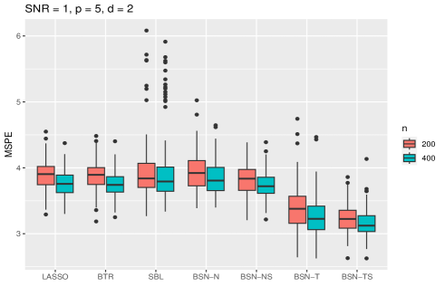
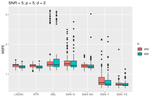
Figure 1: Mean-squared prediction error (MSPE) on test sets for settings with $p=5$ and $d=2$ under SNR = 1 (left panel) and SNR = 5 (right panel), from 100 runs of Part (1) of the experiment.

Figure 1 shows the mean-squared prediction error (MSPE) on the test sets for each method, obtained from 100 runs of the experiment. To better visualize the differences among the better performing methods, we exclude LS and FCR from the subsequent analysis due to their poor performance across all settings. LS severely overfits the training data. FCR uses partial correlations as features which can be computed from correlations between ROIs. This disregards the information contained in the within-ROI variances that can be important for making accurate predictions.

Panel (a) of Figure 1 presents results from Part (1) across training sample sizes ($n$). As $n$ increases from $200$ to $400$, performance improves for all methods, with lower MSPEs on average and reduced variability of the MSPEs. The proposed BSN-TS shows the best performance, achieving the lowest average MSPE among all techniques accompanied by a low level of variance. Within BSN approaches, methods based on the tangent space model (BSN-T and BSN-TS) outperforms the ones using the naive model (BSN-N and BSN-NS). By comparing BSN-T and BSN-TS, we can observe the performance gain by incorporating sparse sampling to $\bm{\Gamma}$. Panel (b) of Figure 1 compares model performance when perturbation was introduced into the data generation process for the case with $n=200$ and SNR = 1. As the noise level ($\nu$) increases, the predictive accuracy declines for all methods. BSN-TS continues to achieve the lowest MSPEs at all perturbation levels.

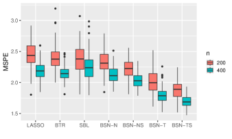
(a) Part (1)

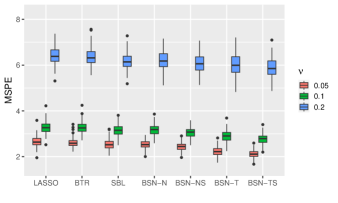
(b) Part (2)

Figure 1: Mean-squared prediction error (MSPE) on test sets for settings with $p=15$ and $d=4$ from 100 runs of Part (1) (left panel) and Part (2) (right panel) of the experiment.

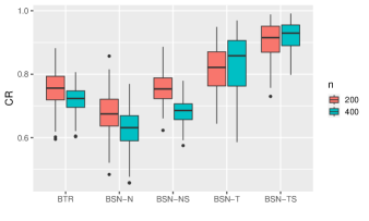
(a) Part (1)

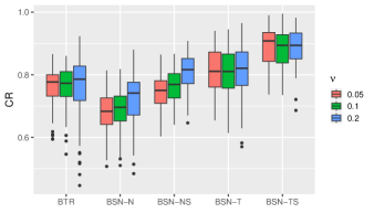
(b) Part (2)

Figure 2: Coverage (CR) on test sets for settings with $p=15$ and $d=4$ from 100 runs of Part (1) (left panel) and Part (2) (right panel) of the experiment.

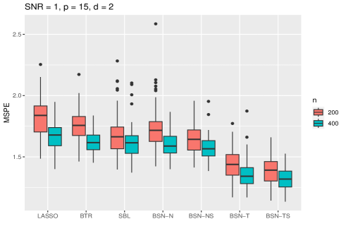
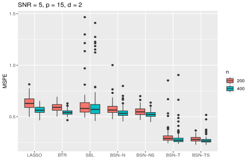
Figure 2: Mean-squared prediction error (MSPE) on test sets for settings with $p=15$ and $d=2$ under SNR = 1 (left panel) and SNR = 5 (right panel), from 100 runs of Part (1) of the experiment

We then compare the coverage rate (CR) for the Bayesian approaches, including BTR and BSN methods, and present the results in Figure 2. In Panel (a) for Part (1), the CRs produced by BST-T and BST-TS are notably higher compared to the other methods. BST-TS achieves the highest CR at roughly 90%, aligning with the specified level (90%) to construct the credible intervals. More training examples slightly improve CR for BSN-T and BSN-TS but for not the other approaches. This results from tightened credible intervals with greater $n$, making it harder for inaccurate interval estimates from the other methods to cover the true values. Panel (b) corresponds to Part (b) of the experiment, fixing $n=200$ while varying the noise level $\nu$. Again BSN-TS produces the highest CRs at around  90%. It is worth noting that the CRs improve with greater noise ($\nu$) for BSN-N and BSN-NS. This results from higher $\nu$ introducing more uncertainty, leading to wider credible intervals that are more likely to capture the true values, though the estimates (e.g. median of the samples) are potentially less accurate.

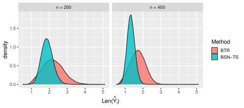
Figure 3: Distribution of $\text{Len}(\hat{Y}_{i})$ produced by BSN-TS and BTR for settings with $p=15$ and $d=4$ from 100 runs of Pat (1) of the experiment.

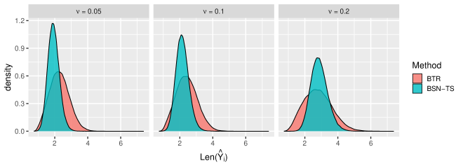
Figure 4: Distribution of $\text{Len}(\hat{Y}_{i})$ produced by BSN-TS and BTR for settings with $p=15$ and $d=4$ from 100 runs of Part (2) of the experiment.

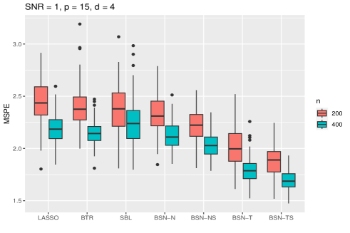
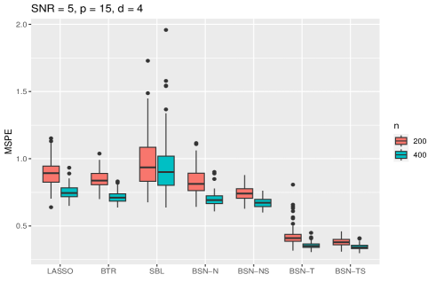
Figure 3: Mean-squared prediction error (MSPE) on test sets for settings with $p=15$ and $d=4$ under SNR = 1 (left panel) and SNR = 5 (right panel), from 100 runs of Part (1) of the experiment

We further analyze the length of 90% credible intervals obtained from BSN methods comparing to BTR. For each run of the experiment, we computed the length $\text{Len}(\hat{Y}_{i})$ from the bayesian approaches under considerations, including all BSN methods and BTR. The lengths were computed for each of the 1000 test data points and we concatenated results from 100 runs of the experiment. Figure 3 displays the distribution of the lengths for BTR and BSN-TS for $n=200$ and 400 separately for Part (1). For both $n$, we observe that BSN-TS tends to produce narrower intervals than BTR, while still achieving better prediction accuracy and coverage (see Figures 1 and 2). The distribution for BSN-TS is more concentrated compared to BTR, suggesting that BSN-TS generates more consistent interval lengths across different runs of the experiment. As the value of $n$ increases, the intervals lengths generated by BSN-TS decreases and the variance of the corresponding distribution also drops.

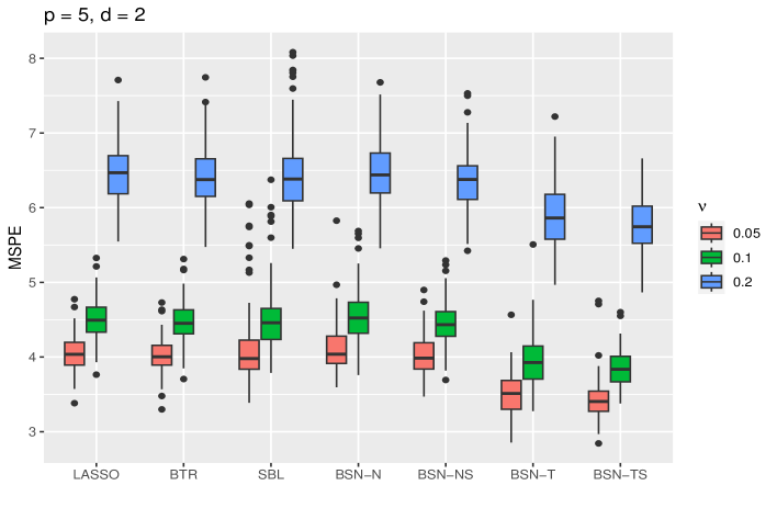
Figure 4: Mean-squared prediction error (MSPE) on test sets for settings with $p=5$ and $d=2$ under SNR = 1 and $n=200$ from 100 runs of Part (2) of the experiment.

The distributions of interval lengths for Part (b) are shown in Figure 4. Similar to Figure 3, the distribution of BSN-TS is more concentrated compared to BTR. As the level of perturbation ($\nu$) grows, the credible intervals from BSN-TS become wider with more variable lengths. With $\nu$ = 0.2, though the average lengths are similar for BSN-TS and BTR, BSN-TS achieves lower MSPEs and higher CRs observed from Figures 1 and 2. From the results in the Appendix, we draw similar conclusions for the other BSN methods under the same settings: their credible intervals are generally narrower than BTR in Parts (1) and Part (2) with $\nu=0.05$ and $0.1$. With $\nu=0.2$, the BSN methods produce credible intervals that are narrower than or similar in length to those from BTR.

Extending our analysis to other settings (see Appendix), we find BSN-TS consistently performs the best in Part (1) and (2). In terms of the MSPE, increasing SNR improves the performance for all methods while SBL’s improvement is less substantial than the others. Despite SBL sharing the same CP decomposition ($\bm{\Gamma}\mathbf{B}\bm{\Gamma}^{T}$) as our model, it shows unstable performance in some cases, producing outlying MSPE values in Part (1). For Part (2), the boxplot patterns are similar to Panel (b) of Figure 2 with BSN-TS achieving the lowest MSPE on average. For CR, BSN-TS continues to be the best performer in Part (1) and (2). While higher SNR improves the CR for BSN-T and BSN-TS, it reduces CR for the other methods since their model yield inaccurate credible intervals even at a lower SNR. Increasing SNR narrows these problematic intervals, worsening the chance to cover the true values.

Regarding the interval length ($\text{Len}(\hat{Y}_{i})$), the performance of BSN-TS and BTR are comparable for $p=5$. With $p=15$, BSN-TS consistently generates narrower credible intervals than BTR, especially under settings with a high SNR (SNR=5) in Part (1). The other BSN methods also yield shorter interval lengths compared to BTR in most cases. In the remaining cases, their lengths are similar to the ones produced by BTR. In Part (2) with added perturbation, we observe similar patterns as in Figure 4: $\text{Len}(\hat{Y}_{i})$ from BSN-TS and BTR are comparable for $\nu=0.2$; BSN-TS produces narrower intervals for $\nu=0.05$ and 0.1. Overall, these results demonstrates BSN-TS’s ability to provide relatively tight and accurate 90% credible intervals across all settings.

4.4.2 Inference on parameters

We focus on analyzing the inference results from BSN-T and BSN-TS since their model aligns with the one in Part (1) of the experiment, for which we know the true values of the parameters. The analyses presented here are for Part (1). We have similar findings from Part (2) and will summarize them in this section and show the complete results in the Appendix.

We compared the absolute cosine similarity (ACS) to access the accuracy in estimating each column of $\bm{\Gamma}$. Figure 5 shows the ACS results for different training sample sizes ($n$). On average, BSN-TS produces higher ACS values than BSN-T, demonstrating its better performance in making inference of $\bm{\Gamma}$. In this $d=4$ setting, we observe lower ACS for $\bm{\gamma}_{2}$ and $\bm{\gamma}_{3}$ compared to $\bm{\gamma}_{1}$ and $\bm{\gamma}_{4}$. This is due to the higher scale of the coefficients $b_{1}$ and $b_{4}$ (versus $b_{2}$ and $b_{3}$) enables easier recovery of the corresponding $\bm{\Gamma}$ columns, since they contribute more signal to construct the responses. Increasing $n$ from 200 to 400 improves the ACS for all $\bm{\gamma}_{j}$’s, especially for $\bm{\gamma}_{2}$ and $\bm{\gamma}_{3}$.

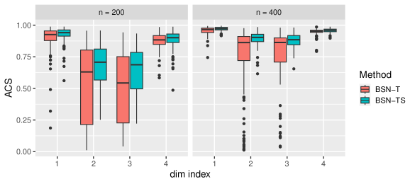
Figure 5: Absolute cosine similarity (ACS) for settings with $p=15$ and $d=4$ from 100 runs of Part (1) of the experiment. The x-axis denotes the indices of the columns of $\bm{\Gamma}$.

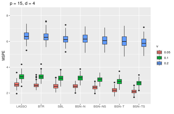
Figure 6: Mean-squared prediction error (MSPE) on test sets for settings with $p=15$ and $d=4$ under SNR = 1 and $n=200$ from 100 runs of Part (2) of the experiment.

We computed the coverage (Cover) for each entry $r_{j,k}$ and averaged the values across 100 runs. For each of BSN-T and BSN-TS, this produces an average coverage matrix of dimension $p\times d$. For easier comparison and visualization, we flattened these matrices into vectors column-wise and plotted the values in Figure 6. The x-axis represents the indices of the vectorized average coverage matrices. We observe that BSN-TS yields higher average coverage than BSN-T for most entries. The values produced by BSN-TS are close to 90%, our specified credible level. In contrast, BSN-T yields some outlying values, with a few even below 50%, showing that it is less stable compared to BSN-TS. The coverage patterns are similar for $n=200$ and $n=400$, with BSN-TS consistently achieving higher and more stable average coverage of the true $\bm{\Gamma}$.

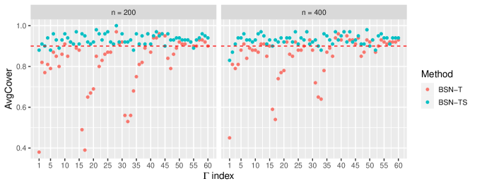
Figure 6: Coverage (Cover) of the entries in $\bm{\Gamma}$ for settings with $p=15$ and $d=4$, averaged for 100 runs of Part (1) of the experiment.

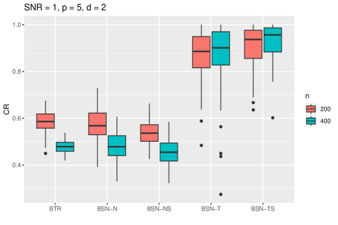
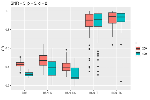
Figure 7: Coverage rate (CR) on test sets for settings with $p=5$ and $d=2$ under SNR = 1 (left panel) and SNR = 5 (right panel), from 100 runs of Part (1) of the experiment.

Figure 7 shows the average coverage of the diagonal entries of $\bm{B}$, namely $b_{1}$ to $b_{4}$. Similar to what is observed for $\bm{\Gamma}$, BSN-TS yields average coverage values close to 90% for all $b_{j}$’s, overall higher than BSN-T. This holds for training sample sizes of $n=200$ and $n=400$.

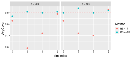
Figure 7: Coverage (Cover) of the diagonal entries in $\mathbf{B}$ for settings with $p=15$ and $d=4$, averaged for 100 runs of Part (1) of the experiment.

From the other settings covered in the Appendix, we find that BSN-TS consistently achieves higher ACS than BSN-T in Part (1) and (2). Similar to our observations from Figure 6 and Figure 7, the average coverage of $\bm{\Gamma}$ and $\bf{B}$ produced by BSN-TS stays close to 90% across all Part (1) cases, outperforming BSN-T. Under perturbations in Part (2), BSN-TS’s average coverage values remain near 90% with a a few entries slightly below the non-perturbed scenarios. By contrast, BSN-T produces quite low average coverage for many entries with some under 50% for $\bm{\Gamma}$.

5 Human Connectome Project

In this section, we present an application of our proposal (BSN-TS) to data from the Human Connectome Project (HCP) and compare it with the alternatives considered in Section 4. The results are provided for the predictive performance and inference on the key ROIs contributing to predicting the age adjusted Picture Vocabulary score (Pic Vocab).

5.1 Data description

We studied the resting-state functional magnetic resonance imaging (rs-fMRI) data from the Human Connectome Project (HCP) S1200 release (Van Essen et al., 2013), which consists of behavioural and imaging data collected from healthy adults between age of 22-35. For each subject, the rs-fMRI data were collected over four complete 15-minute sessions, with 1200 timepoints per session (TR = 750 ms). Each 15-minute run of the rs-fMRI data was preprocessed according to Smith et al. (2013) prior to analysis.

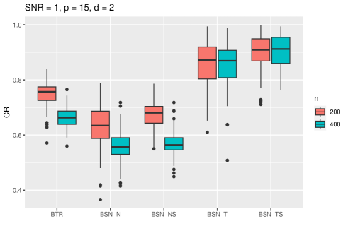
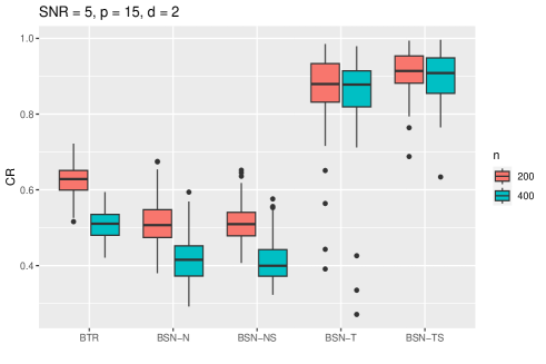
Figure 8: Coverage rate (CR) on test sets for settings with $p=15$ and $d=2$ under SNR = 1 (left panel) and SNR = 5 (right panel), from 100 runs of Part (1) of the experiment.

To convert the rs-fMRI data into time series mapped onto spatial brain regions, we adopted a data-driven parcellation based on group spatial independent component analysis (ICA) (McKeown et al., 1998; Calhoun et al., 2001) with $p=15$ components described as ICA maps (Filippini et al., 2009). The most relevant axial slices for each region in the MNI-152 space (Evans et al., 1993; Mazziotta et al., 1995, 2001) are displayed in Figure 8. The output from the parcellation is contained in the publicly available PTN (Parcellation + Timeseries + Netmats) dataset , which includes data for N=1003 subjects from the S1200 data release. Our study analyzes the rs-fMRI signals in the form of time series from this PTN data.

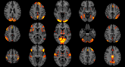
Figure 8: The 15 independent components (ICs) from spatial group-ICA. The components are denoted as Node 1 to 15, provided by the PTN dataset form the S1200 HCP release.

Considering the temporal dependency in the time series , we performed thinning of the observed data based on the effective sample size (ESS) for each subject $i$, similar to the procedure described in Park (2023):

$$\text{ESS}(i)=\min_{j\in\{1,...,p\}}\frac{T_{i}}{1+2\sum_{t=1}^{T_{i}-1}\text{cor}(x_{i,j}(t),x_{i,j}(1+t))},$$

where $x_{i,j}(t)$ denotes the signal at time $t$ in region $j$ for subject $i$. The $\text{EES}(i)$ values range from 181 to 763, with an average of 349 across subjects. We subsampled $\text{EES}(i)$ time points for each subject $i$. The resulting thinned signals for subject $i$ were then used to compute the covariance matrix $\mathbf{M}_{i}$.

The response variable we used is the age-adjusted Picture Vocabulary scores (Pic Vocab) available in the HCP data. These scores were collected from the NIH Toolbox Picture Vocabulary Test (Gershon et al., 2013), In this test, each participant hears a word and selects from four images on the computer screen the one that best depicts its meaning. The results are aggregated for different words and adjusted for participants’ ages to create a final score.

5.2 Implementation details

We compared the performance of the same methods considered in Section 4, including LS, LASSO, FCR, BTR, SBL, and BSN. The implementation details for LS, LASSO, and FCR are identical to the simulation study. We randomly split the data into a training set with either $n=300$ or 800 subjects, and used the remaining subjects as the test set. We report prediction results separately for each training sample size. For BTR and SBL, we fit the models with rank set to 2, 3, and 4. For BSN we try values of $d=2,3,$ and 4. For each of BTR, SBL, BSN-N, BSN-NS, BSN-T, and BSN-TS, we report results using the rank or $d$ value that achieves the lowest mean squared prediction error (MSPE) across 50 runs of the experiment, with each run fitted using a random data split. The selected parameters are rank 3 ($n=300$) and rank 4 ($n=800$) for BTR; rank 2 for SBL and $d=4$ for all BSN methods at both $n$ values.

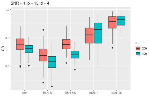
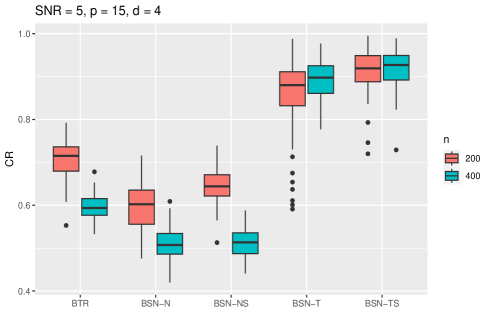
Figure 9: Coverage rate (CR) on test sets for settings with $p=15$ and $d=4$ under SNR = 1 (left panel) and SNR = 5 (right panel), from 100 runs of Part (1) of the experiment.

The original scale of the covariance matrices $\mathbf{M}_{i}$’s in the HCP data are on a higher order of magnitude compared to their tangent space representations $\phi_{\mathbf{M}^{\ast}}(\mathbf{M}_{i})$. To make the scales comparable, we divided all entries in $\mathbf{M}_{i}$ by $10^{4}$, which is equivalent to dividing the time series by $10^{2}$. This allows a fair comparison between BSN with the naive parameterization (BSN-N and BSN-NS) and the tangent representation (BSN-T and BSN-TS) fitted with the same prior on $\mathbf{B}$. Figure 9 shows an example of $\mathbf{M}_{i}$, $\mathbf{M}^{\ast}$, and $\phi_{\mathbf{M}^{\ast}}(\mathbf{M}_{i})$ in Panels (a) to (c) respectively, where $\phi_{\mathbf{M}^{\ast}}(\mathbf{M}_{i})$ is computed based on one random data split and $i$ indexes a random training subject. We can observe that $\phi_{\mathbf{M}^{\ast}}(\mathbf{M}_{i})$ removes some shared structure between $\mathbf{M}_{i}$ and $\mathbf{M}^{\ast}$. We also standardized the response variable, Pic Vocab, to have mean zero and unit variance. This helps in specifying sensible priors for the BSN methods (e.g. a mean zero prior on $\mu$). The priors we used for BSN methods remain unchanged from Section 4. For each BSN method, we ran two MCMC chains with 1500 warming up iterations and 500 sampling iterations for each chain. We tested $\tau=0.1,0.2,$ and 0.3 for BSN-NS and BSN-TS, and report the results for $\tau=0.3$ that yields the best predictive performance.

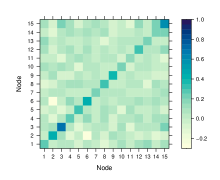
(a) $\mathbf{M}_{i}$

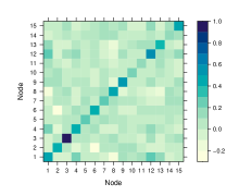
(b) $\mathbf{M}^{\ast}$

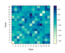
(c) $\phi_{\mathbf{M}^{\ast}}(\mathbf{M}_{i})$

Figure 9: Data illustration of $\mathbf{M}_{i}$ in Panel (a), $\mathbf{M}^{\ast}$ in Panel (b), and $\phi_{\mathbf{M}^{\ast}}(\mathbf{M}_{i})$ in Panel (c), where $i$ indexes a random subject and $\mathbf{M}^{\ast}$ is computed from a random data split with $n=800$.

To evaluate the predictive performance, we calculated the mean squared prediction error (MSPE) on test sets as given in (18). We also computed the length of the 90% credible intervals for $\hat{Y}_{i}$ as defined in (19) to quantify the uncertainty of the predictions. Since the true parameters and the expectation of $Y_{i}$’s are unknown, we do not report the other metrics (CR, ACS, and Cover) considered in Section 4. To provide interpretations and identify key regions predictive of the response based on Section 3, we made inference on the matrix $\bm{\Gamma}^{T}{\mathbf{M}^{\ast}}^{-1/2}$ using MCMC samples of $\bm{\Gamma}$. We then examined if the identified key regions have meaningful interpretations from the neuroscience literature.

5.3 Results

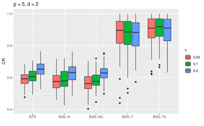
Figure 10: Coverage rate (CR) on test sets for settings with $p=5$, $d=2$, $n=200$, and SNR = 1 from 100 runs of Part (2) of the experiment.

Figure 10 shows the mean-squared prediction error (MSPE) computed on test sets across 50 random data splits with varying training sample sizes ($n$). The y-axis is truncated at 370 to exclude some outlying values from LS and SBL. On average, BSN-TS achieves the best performance for both $n=300$ and $n=800$. With a small sample size $n=300$, LS and SBL performs poorly, likely due to insufficient regularization. Increasing $n$ improves predictions for all methods. Among the BSN approaches, those modelling in the tangent space (BSN-T and BSN-TS) outperform those based on the native model (BSN-N and BSN-NS), suggesting the advantages of accounting for the Riemannian geometry of SPD matrices. Additionally, the sparse sampling methods (BSN-NS and BSN-TS) achieve better prediction accuracy than their non-sparse counterparts (BSN-N and BSN-T), demonstrating the performance improvement achieved by regularizing $\bm{\Gamma}$.

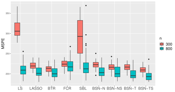
Figure 10: Mean-squared prediction error (MSPE) on test sets obtained from 50 random data splits.

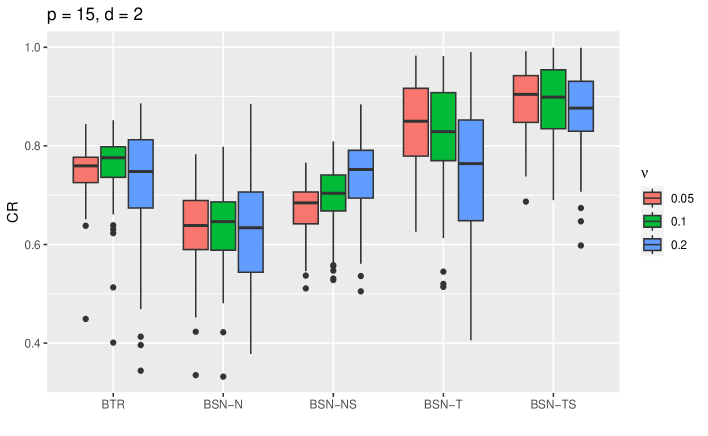
Figure 11: Coverage rate (CR) on test sets for settings with $p=15$, $d=2$, $n=200$, and SNR = 1 from 100 runs of Part (2) of the experiment.

Figure 11 compares the distributions of 90% credible interval lengths for $\hat{Y}_{i}$ computed from BTR versus BSN-TS. The density plots were generated from results aggregated across all test sets over 50 data splits. The x-axis is truncated to exclude some especially wide intervals generated by BTR. We observe that BSN-TS produces more concentrated distributions compared to the heavy-tailed distribution from BTR. This distinction is more notable at a larger sample size of $n=800$, where on average BSN-TS yields narrower credible intervals.

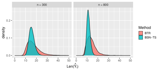
Figure 11: Density plot of $\text{Len}(\hat{Y}_{i})$ produced by BTR and BSN-TS with results combined from 50 runs, each with a random data split.

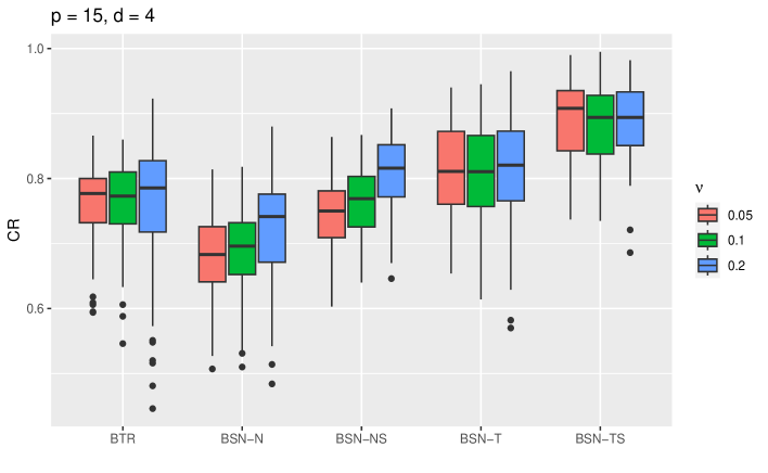
Figure 12: Coverage rate (CR) on test sets for settings with $p=15$, $d=4$, $n=200$, and SNR = 1 from 100 runs of Part (2) of the experiment.

For the inference of parameters, we show in Figure 12 the posterior mean estimates of $\bm{\Gamma}\mathbf{B}\bm{\Gamma}^{T}$ along with the rank-1 components $b_{j}\bm{\gamma}_{j}\bm{\gamma}j^{T}$ for $j=1,...,4$, that constructs this matrix. The averages were taken over all MCMC samples combined from 50 runs. We view $\bm{\Gamma}\mathbf{B}\bm{\Gamma}^{T}$ as the coefficient matrix for $\phi_{\mathbf{M}^{\ast}}(\mathbf{M}_{i})$ and observe that each rank-1 matrix focuses on extracting predictive information from different entries in $\phi_{\mathbf{M}^{\ast}}(\mathbf{M}_{i})$. All components are then combined into a rank-4 coefficient matrix $\bm{\Gamma}\mathbf{B}\bm{\Gamma}^{T}$ that provides flexibility to model the potentially complex mapping from $\phi_{\mathbf{M}^{\ast}}(\mathbf{M}_{i})$ to $Y_{i}$.

Figure 12: Posterior mean of $b_{1}\gamma_{1}\gamma_{1}^{T}$, $b_{2}\gamma_{2}\gamma_{2}^{T}$, $b_{3}\gamma_{3}\gamma_{3}^{T}$, $b_{4}\gamma_{4}\gamma_{4}^{T}$ , and $\bm{\Gamma}\mathbf{B}\bm{\Gamma}^{T}$ computed from MCMC samples across the 50 runs, each with a different random data split.

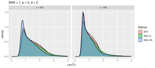
Figure 13: Lengths of the 90% credible intervals for settings with $p=5$ and $d=2$ under SNR = 1 from 100 runs of Part (1) of the experiment. The densities displayed are produced by BTR, BSN-N and BSN-NS.

We then make inferences of $\bm{\Gamma}^{T}{\mathbf{M}^{\ast}}^{-1/2}$, which extracts source signals from the original signals as illustrated in Section 3. Similar to the analysis in Section 4, we aligned the sign of each $\bm{\Gamma}$ column before examining the results. Specifically, for each column of $\bm{\Gamma}$, we found the element that on average has the latest absolute value across all MCMC samples from 50 runs. These elements correspond to Nodes 10, 2, 15, and 14 for the 1st through 4th columns of $\bm{\Gamma}$, respectively. Figure 13 shows the posterior mean of $\bm{\Gamma}^{T}{\mathbf{M}^{\ast}}^{-1/2}$ with the sign-adjusted $\bm{\Gamma}$ samples. From this figure, the regions we identified as important are Nodes 7, 10, 14, and 15, corresponding to entries in Figure 13 with large scales. Referencing the neuroscience study by Smith et al. (2011), these regions relate to the sensorimotor network (Node 7), cognition-language network (Nodes 10 and 14), and default network (Node 15). In particular, given that we are predicting language skills measured as Pic Vocab, it is sensible that cognition-language nodes emerged as significant, aligning with our intuitive expectations.

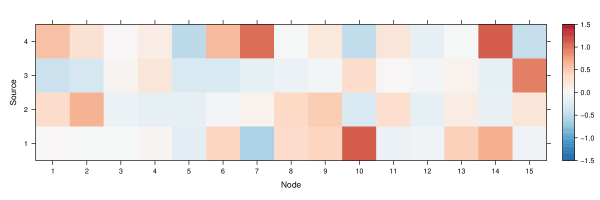
Figure 13: Posterior mean of $\bm{\Gamma}^{T}{\mathbf{M}^{\ast}}^{-1/2}$ computed from aggregated MCMC samples across the 50 runs, each with a random data split.

6 Discussion

In summary, we proposed a Bayesian regression method for associating scalar responses with network predictors measured as SPD matrices. Unlike other Bayesian approaches, our method accounts for the Riemannian geometry of SPD matrices by modelling them in the tangent space. To reduce the number of parameters in the model, our method performs dimension reduction in the tangent space, resulting in a form that resembles the fixed-rank decomposition (Kolda and Bader, 2009) typically found in tensor regression. While existing tangent space approaches (e.g. Dadi et al. (2019) and Pervaiz et al. (2020)) are difficult to interpret, our model allows identifying important brain regions related to the response. Moreover, by introducing sparse sampling on the Stiefel manifold, we obtain parsimonious estimates that effectively avoid overfitting.

From our numerical experiments, we made several key observations. Our proposed method (BSN-TS) achieves the best predictive performance and inference results in the simulation study, with data either generated from our model or with different levels of deviations. Compared to the competing Bayesian proposal (BTR), our method obtains lower prediction errors with shorter credible intervals. Additionally, comparing the proposed BSN-TS with the other variants (BSN-N, BSN-NS, and BSN-T) demonstrates the advantages of sparsity sampling and modelling in the tangent space. Finally, in the case study analyzing HCP data, the proposed method exhibits the best prediction accuracy while identifying regions that are important for predicting Picture Vocabulary scores.

Building on the strengths mentioned above, there are several ways we could further enhance or extend our proposal. Our implementation of BSN-TS adopts a fixed global shrinkage parameter $\tau$ in the horseshoe prior that needs to be specified by the user. We have found in the simulation study that a higher $p$ prefers larger values of $\tau$. This aligns with the intuition that as $p$ rises, the number of angles in the Givens rotations grows, introducing more multiplicative sinusoidal terms. Consequently, each term likely requires less shrinkage for the overall sparsity level to remain constant. It would be worth exploring placing a hyperprior on $\tau$, as studied by Piironen and Vehtari (2017a), which would automatically control of the level of regularization. Further, although we have focuses on predicting continuous responses, our model can extend to classification and ordinal regression by a simple modification of the likelilihood function. Exploring more flexible and nonlinear model formulations in the reduced dimensional space is also of interest for future work.

Appendix

Appendix A: Proof of Theorem 1

Theorem 1: Let $\bm{\Gamma}_{1}=\left(\bm{\gamma}_{1}^{(1)},...,\bm{\gamma}_{d}^{(1)}\right)\in\mathbb{R}^{p\times d}$ and $\bm{\Gamma}_{2}=\left(\bm{\gamma}_{1}^{(2)},...,\bm{\gamma}_{d}^{(2)}\right)\in\mathbb{R}^{p\times d}$ satisfy $\bm{\Gamma}_{1}^{T}\bm{\Gamma}_{1}=\bm{\Gamma}_{2}^{T}\bm{\Gamma}_{2}=\mathbf{I}_{d}$; $\mathbf{B}_{1}=\text{Diag}(b_{1}^{(1)},...,b_{d}^{(1)})$ and $\mathbf{B}_{2}=\text{Diag}(b_{1}^{(2)},...,b_{d}^{(2)})$; and $\mu_{1},\mu_{2}\in\mathbb{R}$. If

$$\mu_{1}+\langle\phi_{\mathbf{M}^{\ast}}(\mathbf{M}),\bm{\Gamma}_{1}\mathbf{B}_{1}\bm{\Gamma}_{1}^{T}\rangle=\mu_{2}+\langle\phi_{\mathbf{M}^{\ast}}(\mathbf{M}),\bm{\Gamma}_{2}\mathbf{B}_{2}\bm{\Gamma}_{2}^{T}\rangle\ \text{for any}\ \mathbf{M}\in\text{Sym}_{p}^{+},$$

then there exist a permutation $\pi(1),...,\pi(d)$ of $1,...,d$, and $l_{j}\in\{0,1\}$ such that for $j=1,...,d$,

$$\bm{\gamma}_{j}^{(1)}=(-1)^{l_{j}}\bm{\gamma}_{\pi(j)}^{(2)},\ b_{j}^{(1)}=b_{\pi(j)}^{(2)},\ \text{and}\ \mu_{1}=\mu_{2}.$$

Proof: $\phi_{\mathbf{M}^{\ast}}(\mathbf{M})$ spans the space of symmetric matrices for $\mathbf{M}\in\text{Sym}_{p}^{+}$ and a fixed $\mathbf{M}^{\ast}$. We first show that $\mu_{1}=\mu_{2}$ by letting $\phi_{\mathbf{M}^{\ast}}(\mathbf{M})=\mathbf{0}_{p}$. Under this condition if

$$\mu_{1}+\langle\phi_{\mathbf{M}^{\ast}}(\mathbf{M}),\bm{\Gamma}_{1}\mathbf{B}_{1}\bm{\Gamma}_{1}^{T}\rangle=\mu_{2}+\langle\phi_{\mathbf{M}^{\ast}}(\mathbf{M}),\bm{\Gamma}_{2}\mathbf{B}_{2}\bm{\Gamma}_{2}^{T}\rangle,$$

then $\mu_{1}=\mu_{2}$.

Next, for any symmetric matrix $\phi_{\mathbf{M}^{\ast}}(\mathbf{M})$, if

$$\langle\phi_{\mathbf{M}^{\ast}}(\mathbf{M}),\bm{\Gamma}_{1}\mathbf{B}_{1}\bm{\Gamma}_{1}^{T}\rangle=\langle\phi_{\mathbf{M}^{\ast}}(\mathbf{M}),\bm{\Gamma}_{2}\mathbf{B}_{2}\bm{\Gamma}_{2}^{T}\rangle,$$

we have $\bm{\Gamma}_{1}\mathbf{B}_{1}\bm{\Gamma}=\bm{\Gamma}_{2}\mathbf{B}_{2}\bm{\Gamma}_{2}^{T}$. Since $\bm{\Gamma}_{1}^{T}\bm{\Gamma}_{1}=\bm{\Gamma}_{2}^{T}\bm{\Gamma}_{2}=\mathbf{I}_{d}$ and $\mathbf{B}_{1}$ and $\mathbf{B}_{2}$ are diagonal matrixes, $\bm{\Gamma}_{1}\mathbf{B}_{1}\bm{\Gamma}$ and $\bm{\Gamma}_{2}\mathbf{B}_{2}\bm{\Gamma}$ represent eigenvalue decompositions. The eigenvectors are the columns of $\mathbf{\Gamma}_{1}$ and $\mathbf{\Gamma}_{2}$, and the eigenvalues are the diagonal elements of $\mathbf{B}_{1}$ and $\mathbf{B}_{2}$. Such decompositions are unique up to permutations of eigenvectors together with the corresponding eigenvalues, and sign flips of each eigenvector, and thus completes the proof.

Appendix B: Predictive performance

Mean-squared prediction error (MSPE)

Figure 5: Mean-squared prediction error (MSPE) on test sets for settings with $p=15$ and $d=2$ under SNR = 1 and $n=200$ from 100 runs of Part (2) of the experiment.

Coverage rate (CR)

Len$(\hat{Y_{i}})$

In what follows we show the density plots of the lengths of the 90% credible intervals for different settings. For easier comparison with BTR and among the BSN methods, while avoiding many densities in the same figure, for each case we make two plots; both have the same BTR density, and for BSN, one plot has BSN-N and BSN-NS, and the other has BSN-T and BSN-TS. The x-axis in some figures is right truncated to exclude the density estimated from a few very large intervals, allowing for easier comparison of the majority of the interval lengths on the same plot.

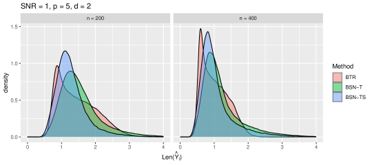
Figure 14: Lengths of the 90% credible intervals for settings with $p=5$ and $d=2$ under SNR = 1 from 100 runs of Part (1) of the experiment. The densities displayed are produced by BTR, BSN-T and BSN-TS.

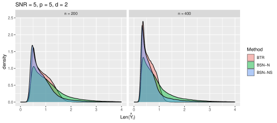
Figure 15: Lengths of the 90% credible intervals for settings with $p=5$ and $d=2$ under SNR = 5 from 100 runs of Part (1) of the experiment. The densities displayed are produced by BTR, BSN-N and BSN-NS.

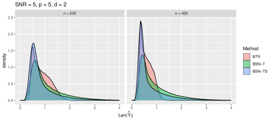
Figure 16: Lengths of the 90% credible intervals for settings with $p=5$ and $d=2$ under SNR = 5 from 100 runs of Part (1) of the experiment. The densities displayed are produced by BTR, BSN-T and BSN-TS.

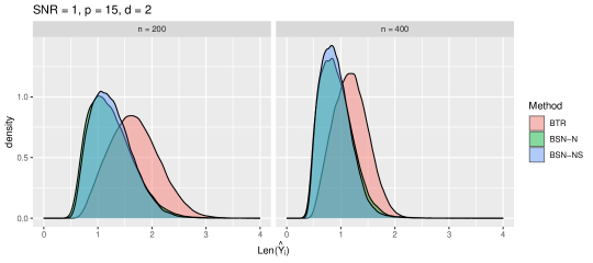
Figure 17: Lengths of the 90% credible intervals for settings with $p=15$ and $d=2$ under SNR = 1 from 100 runs of Part (1) of the experiment. The densities displayed are produced by BTR, BSN-N and BSN-NS.

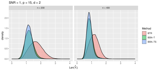
Figure 18: Lengths of the 90% credible intervals for settings with $p=15$ and $d=2$ under SNR = 1 from 100 runs of Part (1) of the experiment. The densities displayed are produced by BTR, BSN-T and BSN-TS.

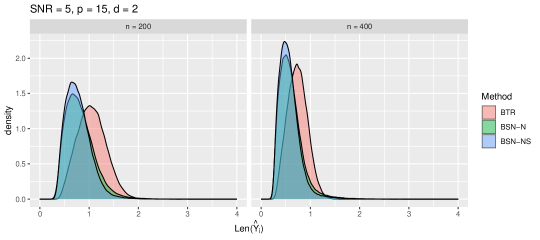
Figure 19: Lengths of the 90% credible intervals for settings with $p=15$ and $d=2$ under SNR = 5 from 100 runs of Part (1) of the experiment. The densities displayed are produced by BTR, BSN-N and BSN-NS.

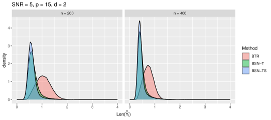
Figure 20: Lengths of the 90% credible intervals for settings with $p=15$ and $d=2$ under SNR = 5 from 100 runs of Part (1) of the experiment. The densities displayed are produced by BTR, BSN-T and BSN-TS.

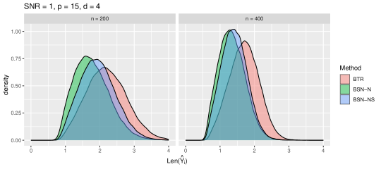
Figure 21: Lengths of the 90% credible intervals for settings with $p=15$ and $d=4$ under SNR = 1 from 100 runs of Part (1) of the experiment. The densities displayed are produced by BTR, BSN-N and BSN-NS.

Figure 22: Lengths of the 90% credible intervals for settings with $p=15$ and $d=2$ under SNR = 1 from 100 runs of Part (1) of the experiment. The densities displayed are produced by BTR, BSN-T and BSN-TS.

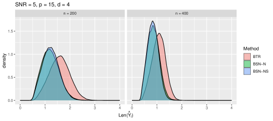
Figure 23: Lengths of the 90% credible intervals for settings with $p=15$ and $d=4$ under SNR = 5 from 100 runs of Part (1) of the experiment. The densities displayed are produced by BTR, BSN-N and BSN-NS.

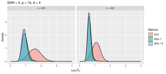
Figure 24: Lengths of the 90% credible intervals for settings with $p=15$ and $d=4$ under SNR = 5 from 100 runs of Part (1) of the experiment. The densities displayed are produced by BTR, BSN-T and BSN-TS.

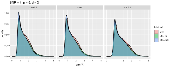
Figure 25: Lengths of the 90% credible intervals for settings with $p=5$ and $d=2$, $n=200$, and SNR = 1 from 100 runs of Part (2) of the experiment. The densities displayed are produced by BTR, BSN-N and BSN-NS.

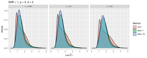
Figure 26: Lengths of the 90% credible intervals for settings with $p=5$ and $d=2$, $n=200$, and SNR = 1 from 100 runs of Part (2) of the experiment. The densities displayed are produced by BTR, BSN-T and BSN-TS.

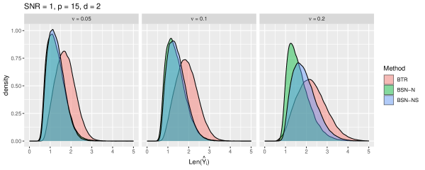
Figure 27: Lengths of the 90% credible intervals for settings with $p=15$ and $d=2$, $n=200$, and SNR = 1 from 100 runs of Part (2) of the experiment. The densities displayed are produced by BTR, BSN-N and BSN-NS.

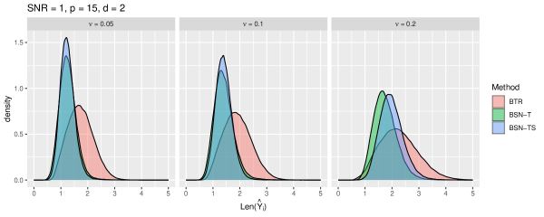
Figure 28: Lengths of the 90% credible intervals for settings with $p=15$ and $d=2$, $n=200$, and SNR = 1 from 100 runs of Part (2) of the experiment. The densities displayed are produced by BTR, BSN-T and BSN-TS.

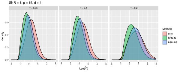
Figure 29: Lengths of the 90% credible intervals for settings with $p=15$ and $d=4$, $n=200$, and SNR = 1 from 100 runs of Part (2) of the experiment. The densities displayed are produced by BTR, BSN-N and BSN-NS.

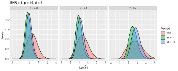
Figure 30: Lengths of the 90% credible intervals for settings with $p=15$ and $d=4$, $n=200$, and SNR = 1 from 100 runs of Part (2) of the experiment. The densities displayed are produced by BTR, BSN-T and BSN-TS.

Appendix C: Inference of parameters

For the absolute cosine similarity (ACS) metric, in some cases, the y-axis is truncated from the bottom to better visualize the differences between BSN-T and BSN-TS. The outlying values that fall outside the displayed range on the truncated y-axis are all from BSN-T.

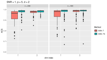
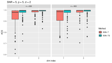
Figure 31: Absolute cosine similarity (ACS) for settings with $p=5$ and $d=2$ under SNR = 1 (left panel) and SNR = 5 (right panel), from 100 runs of Part (1) of the experiment.

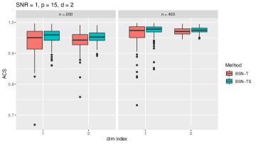
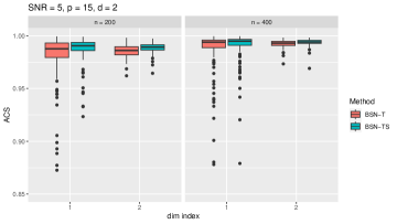
Figure 32: Absolute cosine similarity (ACS) for settings with $p=15$ and $d=2$ under SNR = 1 (left panel) and SNR = 5 (right panel), from 100 runs of Part (1) of the experiment.

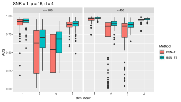
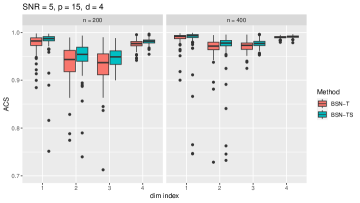
Figure 33: Absolute cosine similarity (ACS) for settings with $p=15$ and $d=4$ under SNR = 1 (left panel) and SNR = 5 (right panel), from 100 runs of Part (1) of the experiment.

Figure 34: Absolute cosine similarity (ACS) for settings with $p=5$, $d=2$, $n=200$ and SNR = 1 from 100 runs of Part (2) of the experiment.

Figure 35: Absolute cosine similarity (ACS) for settings with $p=15$, $d=2$, $n=200$ and SNR = 1 from 100 runs of Part (2) of the experiment.

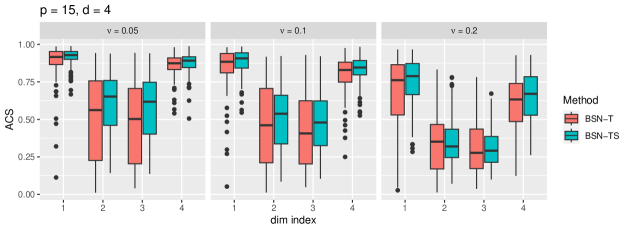
Figure 36: Absolute cosine similarity (ACS) for settings with $p=15$, $d=4$, $n=200$ and SNR = 1 from 100 runs of Part (2) of the experiment.

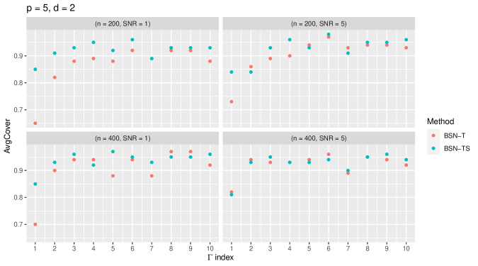
Figure 37: Coverage (Cover) of the entries in $\bm{\Gamma}$ for settings with $p=5$ and $d=2$, averaged for 100 runs of Part (1) of the experiment.

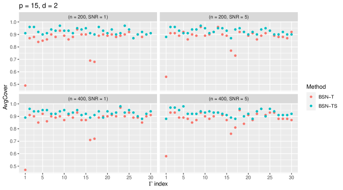
Figure 38: Coverage (Cover) of the entries in $\bm{\Gamma}$ for settings with $p=15$ and $d=2$, averaged for 100 runs of Part (1) of the experiment.

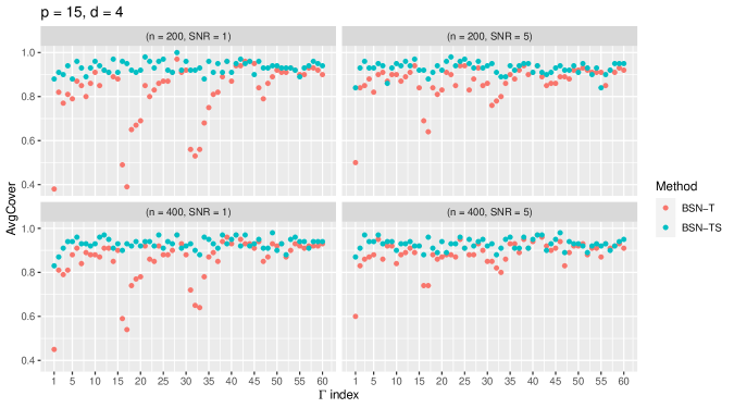
Figure 39: Coverage (Cover) of the entries in $\bm{\Gamma}$ for settings with $p=15$ and $d=4$, averaged for 100 runs of Part (1) of the experiment.

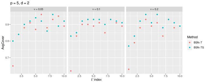
Figure 40: Coverage (Cover) of the entries in $\bm{\Gamma}$ for settings with $p=5$, $d=2$, $n=200$, and SNR = 1, averaged for 100 runs of Part (2) of the experiment.

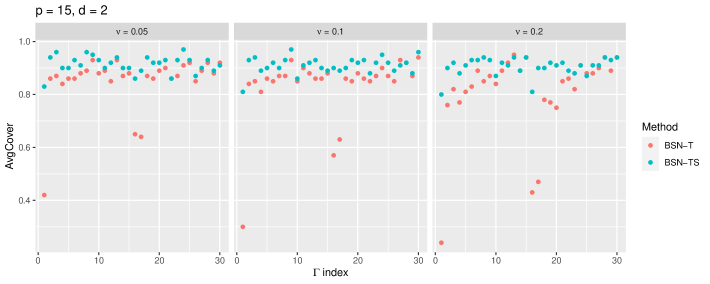
Figure 41: Coverage (Cover) of the entries in $\bm{\Gamma}$ for settings with $p=15$, $d=2$, $n=200$, and SNR = 1, , averaged for 100 runs of Part (2) of the experiment.

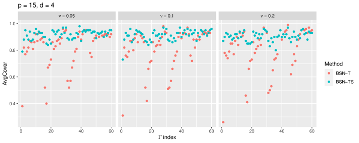
Figure 42: Coverage (Cover) of the entries in $\bm{\Gamma}$ for settings with $p=15$, $d=4$, $n=200$, and SNR = 1, averaged for 100 runs of Part (2) of the experiment.

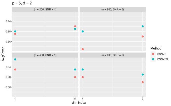
Figure 43: Coverage (Cover) of the diagonal entries in $\mathbf{B}$ for settings with $p=5$ and $d=2$, averaged for 100 runs of Part (1) of the experiment.

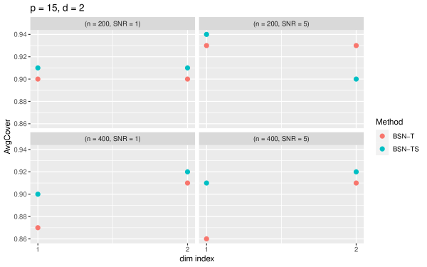
Figure 44: Coverage (Cover) of the diagonal entries in $\mathbf{B}$ for settings with $p=15$ and $d=2$, averaged for 100 runs of Part (1) of the experiment.

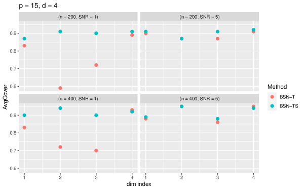
Figure 45: Coverage (Cover) of the diagonal entries in $\mathbf{B}$ for settings with $p=15$ and $d=4$, averaged for 100 runs of Part (1) of the experiment.

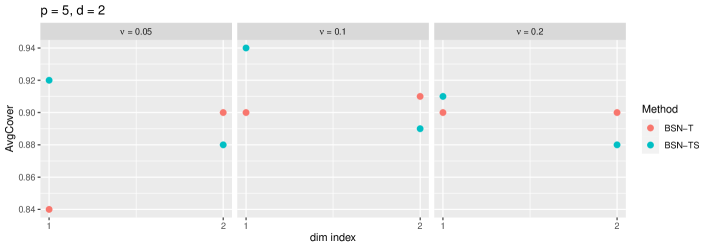
Figure 46: Coverage (Cover) of the diagonal entries in $\mathbf{B}$ for settings with $p=5$, $d=2$, $n=200$, and SNR = 1, averaged for 100 runs of Part (2) of the experiment.

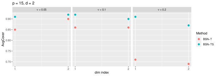
Figure 47: Coverage (Cover) of the diagonal entries in $\mathbf{B}$ for settings with $p=15$, $d=2$, $n=200$, and SNR = 1, , averaged for 100 runs of Part (2) of the experiment.

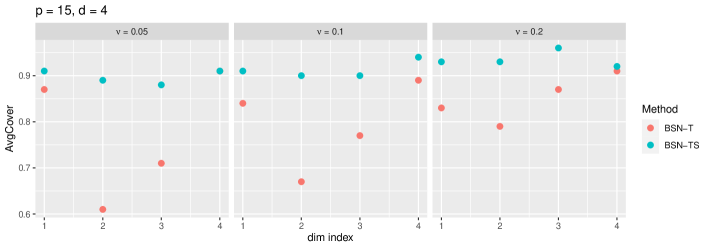
Figure 48: Coverage (Cover) of the diagonal entries in $\mathbf{B}$ for settings with $p=15$, $d=4$, $n=200$, and SNR = 1, averaged for 100 runs of Part (2) of the experiment.

References

- Bastos and Schoffelen (2016) André M Bastos and Jan-Mathijs Schoffelen. A tutorial review of functional connectivity analysis methods and their interpretational pitfalls. Frontiers in systems neuroscience, 9:175, 2016.
- Borchers (2022) Hans W. Borchers. pracma: Practical Numerical Math Functions, 2022. URL https://CRAN.R-project.org/package=pracma. R package version 2.4.2.
- Brzyski et al. (2023) Damian Brzyski, Xixi Hu, Joaquín Goñi, Beau Ances, Timothy W Randolph, and Jaroslaw Harezlak. Matrix-variate regression for sparse, low-rank estimation of brain connectivities associated with a clinical outcome. IEEE Transactions on Biomedical Engineering, 2023.
- Bullmore and Sporns (2009) Ed Bullmore and Olaf Sporns. Complex brain networks: graph theoretical analysis of structural and functional systems. Nature reviews neuroscience, 10(3):186–198, 2009.
- Calhoun et al. (2001) Vince D Calhoun, Tulay Adali, Godfrey D Pearlson, and James J Pekar. A method for making group inferences from functional mri data using independent component analysis. Human brain mapping, 14(3):140–151, 2001.
- Carpenter et al. (2017) Bob Carpenter, Andrew Gelman, Matthew D Hoffman, Daniel Lee, Ben Goodrich, Michael Betancourt, Marcus Brubaker, Jiqiang Guo, Peter Li, and Allen Riddell. Stan: A probabilistic programming language. Journal of statistical software, 76(1), 2017.
- Carvalho et al. (2009) Carlos M Carvalho, Nicholas G Polson, and James G Scott. Handling sparsity via the horseshoe. In Artificial intelligence and statistics, pages 73–80. PMLR, 2009.
- Carvalho et al. (2010) Carlos M Carvalho, Nicholas G Polson, and James G Scott. The horseshoe estimator for sparse signals. Biometrika, 97(2):465–480, 2010.
- Cheon et al. (2003) Gi-Sang Cheon, Suk-Geun Hwang, Seog-Hoon Rim, Bryan L Shader, and Seok-Zun Song. Sparse orthogonal matrices. Linear algebra and its applications, 373:211–222, 2003.
- Craddock et al. (2009) R Cameron Craddock, Paul E Holtzheimer III, Xiaoping P Hu, and Helen S Mayberg. Disease state prediction from resting state functional connectivity. Magnetic Resonance in Medicine: An Official Journal of the International Society for Magnetic Resonance in Medicine, 62(6):1619–1628, 2009.
- Dadi et al. (2019) Kamalaker Dadi, Mehdi Rahim, Alexandre Abraham, Darya Chyzhyk, Michael Milham, Bertrand Thirion, Gaël Varoquaux, Alzheimer’s Disease Neuroimaging Initiative, et al. Benchmarking functional connectome-based predictive models for resting-state fmri. NeuroImage, 192:115–134, 2019.
- Du et al. (2018) Yuhui Du, Zening Fu, and Vince D Calhoun. Classification and prediction of brain disorders using functional connectivity: promising but challenging. Frontiers in neuroscience, 12:525, 2018.
- Evans et al. (1993) Alan C Evans, D Louis Collins, SR Mills, Edward D Brown, Ryan L Kelly, and Terry M Peters. 3d statistical neuroanatomical models from 305 mri volumes. In 1993 IEEE conference record nuclear science symposium and medical imaging conference, pages 1813–1817. IEEE, 1993.
- Fair et al. (2013) Damien A Fair, Joel T Nigg, Swathi Iyer, Deepti Bathula, Kathryn L Mills, Nico UF Dosenbach, Bradley L Schlaggar, Maarten Mennes, David Gutman, Saroja Bangaru, et al. Distinct neural signatures detected for adhd subtypes after controlling for micro-movements in resting state functional connectivity mri data. Frontiers in systems neuroscience, 6:80, 2013.
- Filippini et al. (2009) N Filippini, BJ MacIntosh, MG Hough, GM Goodwin, GB Frisoni, K Ebmeier, S Smith, PM Matthews, CF Beckmann, and CE Mackay. Distinct patterns of brain activity in young carriers of the apoe e4 allele. Neuroimage, 47:S139, 2009.
- Friedman et al. (2010) Jerome Friedman, Trevor Hastie, and Rob Tibshirani. Regularization paths for generalized linear models via coordinate descent. Journal of statistical software, 33(1):1, 2010.
- Gabry et al. (2023) Jonah Gabry, Rok Češnovar, and Andrew Johnson. cmdstanr: R Interface to ’CmdStan’, 2023. https://mc-stan.org/cmdstanr/, https://discourse.mc-stan.org.
- Gaur et al. (2021) Pramod Gaur, Anirban Chowdhury, Karl McCreadie, Ram Bilas Pachori, and Hui Wang. Logistic regression with tangent space-based cross-subject learning for enhancing motor imagery classification. IEEE Transactions on Cognitive and Developmental Systems, 14(3):1188–1197, 2021.
- Gershon et al. (2013) Richard C Gershon, Molly V Wagster, Hugh C Hendrie, Nathan A Fox, Karon F Cook, and Cindy J Nowinski. Nih toolbox for assessment of neurological and behavioral function. Neurology, 80(11 Supplement 3):S2–S6, 2013.
- Guha and Rodriguez (2021) Sharmistha Guha and Abel Rodriguez. Bayesian regression with undirected network predictors with an application to brain connectome data. Journal of the American Statistical Association, 116(534):581–593, 2021.
- Guhaniyogi et al. (2017) Rajarshi Guhaniyogi, Shaan Qamar, and David B Dunson. Bayesian tensor regression. The Journal of Machine Learning Research, 18(1):2733–2763, 2017.
- He et al. (2020) Tong He, Ru Kong, Avram J Holmes, Minh Nguyen, Mert R Sabuncu, Simon B Eickhoff, Danilo Bzdok, Jiashi Feng, and BT Thomas Yeo. Deep neural networks and kernel regression achieve comparable accuracies for functional connectivity prediction of behavior and demographics. NeuroImage, 206:116276, 2020.
- Hung and Wang (2013) Hung Hung and Chen-Chien Wang. Matrix variate logistic regression model with application to eeg data. Biostatistics, 14(1):189–202, 2013.
- Jiang et al. (2020) Bei Jiang, Eva Petkova, Thaddeus Tarpey, and R Todd Ogden. A bayesian approach to joint modeling of matrix-valued imaging data and treatment outcome with applications to depression studies. Biometrics, 76(1):87–97, 2020.
- Kobler et al. (2021) Reinmar J Kobler, Jun-Ichiro Hirayama, Lea Hehenberger, Catarina Lopes-Dias, Gernot R Müller-Putz, and Motoaki Kawanabe. On the interpretation of linear riemannian tangent space model parameters in m/eeg. In 2021 43rd Annual International Conference of the IEEE Engineering in Medicine & Biology Society (EMBC), pages 5909–5913. IEEE, 2021.
- Kolda and Bader (2009) Tamara G Kolda and Brett W Bader. Tensor decompositions and applications. SIAM review, 51(3):455–500, 2009.
- Legendre (1806) Adrien Marie Legendre. Nouvelles méthodes pour la détermination des orbites des comètes: avec un supplément contenant divers perfectionnemens de ces méthodes et leur application aux deux comètes de 1805. Courcier, 1806.
- Li et al. (2018) Xiaoshan Li, Da Xu, Hua Zhou, and Lexin Li. Tucker tensor regression and neuroimaging analysis. Statistics in Biosciences, 10:520–545, 2018.
- Lin et al. (2018) Qi Lin, Monica D Rosenberg, Kwangsun Yoo, Tiffany W Hsu, Thomas P O’Connell, and Marvin M Chun. Resting-state functional connectivity predicts cognitive impairment related to alzheimer’s disease. Frontiers in aging neuroscience, 10:94, 2018.
- Ma et al. (2022) Xin Ma, Suprateek Kundu, and Jennifer Stevens. Semi-parametric bayes regression with network-valued covariates. Machine Learning, 111(10):3733–3767, 2022.
- Mazziotta et al. (2001) John Mazziotta, Arthur Toga, Alan Evans, Peter Fox, Jack Lancaster, Karl Zilles, Roger Woods, Tomas Paus, Gregory Simpson, Bruce Pike, et al. A probabilistic atlas and reference system for the human brain: International consortium for brain mapping (icbm). Philosophical Transactions of the Royal Society of London. Series B: Biological Sciences, 356(1412):1293–1322, 2001.
- Mazziotta et al. (1995) John C Mazziotta, Arthur W Toga, Alan Evans, Peter Fox, Jack Lancaster, et al. A probabilistic atlas of the human brain: theory and rationale for its development. Neuroimage, 2(2):89–101, 1995.
- McKeown et al. (1998) Martin J McKeown, Scott Makeig, Greg G Brown, Tzyy-Ping Jung, Sandra S Kindermann, Anthony J Bell, and Terrence J Sejnowski. Analysis of fmri data by blind separation into independent spatial components. Human brain mapping, 6(3):160–188, 1998.
- Meskaldji et al. (2016) Djalel-Eddine Meskaldji, Maria Giulia Preti, Thomas AW Bolton, Marie-Louise Montandon, Cristelle Rodriguez, Stephan Morgenthaler, Panteleimon Giannakopoulos, Sven Haller, and Dimitri Van De Ville. Prediction of long-term memory scores in mci based on resting-state fmri. NeuroImage: Clinical, 12:785–795, 2016.
- Ming and Kundu (2022) Jin Ming and Suprateek Kundu. Flexible bayesian support vector machines for brain network-based classification. arXiv preprint arXiv:2205.12143, 2022.
- Ng et al. (2015) Bernard Ng, Gael Varoquaux, Jean Baptiste Poline, Michael Greicius, and Bertrand Thirion. Transport on riemannian manifold for connectivity-based brain decoding. IEEE transactions on medical imaging, 35(1):208–216, 2015.
- Papadogeorgou et al. (2021) Georgia Papadogeorgou, Zhengwu Zhang, and David B Dunson. Soft tensor regression. The Journal of Machine Learning Research, 22(1):9981–10033, 2021.
- Papaspiliopoulos et al. (2007) Omiros Papaspiliopoulos, Gareth O Roberts, and Martin Sköld. A general framework for the parametrization of hierarchical models. Statistical Science, pages 59–73, 2007.
- Park (2023) Hyung G Park. Bayesian estimation of covariate assisted principal regression for brain functional connectivity. arXiv preprint arXiv:2306.07181, 2023.
- Pennec et al. (2006) Xavier Pennec, Pierre Fillard, and Nicholas Ayache. A riemannian framework for tensor computing. International Journal of computer vision, 66:41–66, 2006.
- Pervaiz et al. (2020) Usama Pervaiz, Diego Vidaurre, Mark W Woolrich, and Stephen M Smith. Optimising network modelling methods for fmri. Neuroimage, 211:116604, 2020.
- Piironen and Vehtari (2017a) Juho Piironen and Aki Vehtari. On the hyperprior choice for the global shrinkage parameter in the horseshoe prior. In Artificial Intelligence and Statistics, pages 905–913. PMLR, 2017a.
- Piironen and Vehtari (2017b) Juho Piironen and Aki Vehtari. Sparsity information and regularization in the horseshoe and other shrinkage priors. 2017b.
- Pourzanjani et al. (2021) Arya A Pourzanjani, Richard M Jiang, Brian Mitchell, Paul J Atzberger, and Linda R Petzold. Bayesian inference over the stiefel manifold via the givens representation. Bayesian Analysis, 16(2):639–666, 2021.
- R Core Team (2022) R Core Team. R: A Language and Environment for Statistical Computing. R Foundation for Statistical Computing, Vienna, Austria, 2022. URL https://www.R-project.org/.
- Relión et al. (2019) Jesús D Arroyo Relión, Daniel Kessler, Elizaveta Levina, and Stephan F Taylor. Network classification with applications to brain connectomics. The annals of applied statistics, 13(3):1648, 2019.
- Ryali et al. (2012) Srikanth Ryali, Tianwen Chen, Kaustubh Supekar, and Vinod Menon. Estimation of functional connectivity in fmri data using stability selection-based sparse partial correlation with elastic net penalty. NeuroImage, 59(4):3852–3861, 2012.
- Sabbagh et al. (2019) David Sabbagh, Pierre Ablin, Gaël Varoquaux, Alexandre Gramfort, and Denis A Engemann. Manifold-regression to predict from meg/eeg brain signals without source modeling. Advances in Neural Information Processing Systems, 32, 2019.
- Schwartzman (2016) Armin Schwartzman. Lognormal distributions and geometric averages of symmetric positive definite matrices. International statistical review, 84(3):456–486, 2016.
- Smith et al. (2011) Stephen M Smith, Karla L Miller, Gholamreza Salimi-Khorshidi, Matthew Webster, Christian F Beckmann, Thomas E Nichols, Joseph D Ramsey, and Mark W Woolrich. Network modelling methods for fmri. Neuroimage, 54(2):875–891, 2011.
- Smith et al. (2013) Stephen M Smith, Diego Vidaurre, Christian F Beckmann, Matthew F Glasser, Mark Jenkinson, Karla L Miller, Thomas E Nichols, Emma C Robinson, Gholamreza Salimi-Khorshidi, Mark W Woolrich, et al. Functional connectomics from resting-state fmri. Trends in cognitive sciences, 17(12):666–682, 2013.
- Song et al. (2008) Ming Song, Yuan Zhou, Jun Li, Yong Liu, Lixia Tian, Chunshui Yu, and Tianzi Jiang. Brain spontaneous functional connectivity and intelligence. Neuroimage, 41(3):1168–1176, 2008.
- Stewart (1980) Gilbert W Stewart. The efficient generation of random orthogonal matrices with an application to condition estimators. SIAM Journal on Numerical Analysis, 17(3):403–409, 1980.
- Strain et al. (2022) Jeremy F Strain, Matthew R Brier, Aaron Tanenbaum, Brian A Gordon, John E McCarthy, Aylin Dincer, Daniel S Marcus, Jasmeer P Chhatwal, Neill R Graff-Radford, Gregory S Day, et al. Covariance-based vs. correlation-based functional connectivity dissociates healthy aging from alzheimer disease. Neuroimage, 261:119511, 2022.
- Tibshirani (1996) Robert Tibshirani. Regression shrinkage and selection via the lasso. Journal of the Royal Statistical Society Series B: Statistical Methodology, 58(1):267–288, 1996.
- Tomasi and Volkow (2020) Dardo Tomasi and Nora D Volkow. Network connectivity predicts language processing in healthy adults. Human Brain Mapping, 41(13):3696–3708, 2020.
- Van Essen et al. (2013) David C Van Essen, Stephen M Smith, Deanna M Barch, Timothy EJ Behrens, Essa Yacoub, Kamil Ugurbil, Wu-Minn HCP Consortium, et al. The wu-minn human connectome project: an overview. Neuroimage, 80:62–79, 2013.
- Varoquaux et al. (2010) Gaël Varoquaux, Flore Baronnet, Andreas Kleinschmidt, Pierre Fillard, and Bertrand Thirion. Detection of brain functional-connectivity difference in post-stroke patients using group-level covariance modeling. In Medical Image Computing and Computer-Assisted Intervention–MICCAI 2010: 13th International Conference, Beijing, China, September 20-24, 2010, Proceedings, Part I 13, pages 200–208. Springer, 2010.
- Venkataraman et al. (2012) Archana Venkataraman, Thomas J Whitford, Carl-Fredrik Westin, Polina Golland, and Marek Kubicki. Whole brain resting state functional connectivity abnormalities in schizophrenia. Schizophrenia research, 139(1-3):7–12, 2012.
- Vogelstein et al. (2012) Joshua T Vogelstein, William Gray Roncal, R Jacob Vogelstein, and Carey E Priebe. Graph classification using signal-subgraphs: Applications in statistical connectomics. IEEE transactions on pattern analysis and machine intelligence, 35(7):1539–1551, 2012.
- Wang et al. (2019) Lu Wang, Zhengwu Zhang, and David Dunson. Symmetric bilinear regression for signal subgraph estimation. IEEE Transactions on Signal Processing, 67(7):1929–1940, 2019.
- Wang et al. (2021) Lu Wang, Feng Vankee Lin, Martin Cole, and Zhengwu Zhang. Learning clique subgraphs in structural brain network classification with application to crystallized cognition. Neuroimage, 225:117493, 2021.
- Watanabe (2010) Sumio Watanabe. Asymptotic equivalence of bayes cross validation and widely applicable information criterion in singular learning theory. Journal of Machine Learning Research, 11(Dec):3571–3594, 2010.
- Weaver et al. (2023) Caleb Weaver, Luo Xiao, and Martin A Lindquist. Single-index models with functional connectivity network predictors. Biostatistics, 24(1):52–67, 2023.
- You and Park (2021) Kisung You and Hae-Jeong Park. Re-visiting riemannian geometry of symmetric positive definite matrices for the analysis of functional connectivity. NeuroImage, 225:117464, 2021.
- Zeng et al. (2012) Ling-Li Zeng, Hui Shen, Li Liu, Lubin Wang, Baojuan Li, Peng Fang, Zongtan Zhou, Yaming Li, and Dewen Hu. Identifying major depression using whole-brain functional connectivity: a multivariate pattern analysis. Brain, 135(5):1498–1507, 2012.
- Zhang et al. (2014) Mingxia Zhang, Jin Li, Chuansheng Chen, Gui Xue, Zhonglin Lu, Leilei Mei, Hongli Xue, Feng Xue, Qinghua He, Chunhui Chen, et al. Resting-state functional connectivity and reading abilities in first and second languages. NeuroImage, 84:546–553, 2014.
- Zhang et al. (2019) Zhengwu Zhang, Genevera I Allen, Hongtu Zhu, and David Dunson. Tensor network factorizations: Relationships between brain structural connectomes and traits. Neuroimage, 197:330–343, 2019.
- Zhao and Leng (2014) Junlong Zhao and Chenlei Leng. Structured lasso for regression with matrix covariates. Statistica Sinica, pages 799–814, 2014.
- Zhou and Li (2014) Hua Zhou and Lexin Li. Regularized matrix regression. Journal of the Royal Statistical Society. Series B, Statistical Methodology, 76(2):463, 2014.
- Zhou et al. (2013) Hua Zhou, Lexin Li, and Hongtu Zhu. Tensor regression with applications in neuroimaging data analysis. Journal of the American Statistical Association, 108(502):540–552, 2013.