ShaRP: Explaining Rankings with Shapley Values

Abstract

Algorithmic decisions in critical domains such as hiring, college admissions, and lending are often based on rankings. Because of the impact these decisions have on individuals, organizations, and population groups, there is a need to understand them: to know whether the decisions are abiding by the law, to help individuals improve their rankings, and to design better ranking procedures.

In this paper, we present ShaRP (Shapley for Rankings and Preferences), a framework that explains the contributions of features to different aspects of a ranked outcome, and is based on Shapley values. Using ShaRP, we show that even when the scoring function used by an algorithmic ranker is known and linear, the weight of each feature does not correspond to its Shapley value contribution. The contributions instead depend on the feature distributions, and on the subtle local interactions between the scoring features. ShaRP builds on the Quantitative Input Influence framework, and can compute the contributions of features for multiple Quantities of Interest, including score, rank, pair-wise preference, and top-k. Because it relies on black-box access to the ranker, ShaRP can be used to explain both score-based and learned ranking models. We show results of an extensive experimental validation of ShaRP using real and synthetic datasets, showcasing its usefulness for qualitative analysis.

1 Introduction

Algorithmic rankers are broadly used to support decision-making in critical domains, including critical domains such as hiring and employment, school and college admissions, credit and lending, and college ranking. Because of the impact rankers have on individuals, organizations, and population groups, there is a need to understand them: to know whether the decisions are abiding by the law, to help individuals improve their rankings, and to design better ranking procedures. In this paper, we present ShaRP (Shapley for Rankings and Preferences), a framework that explains the contributions of features to different aspects of a ranked outcome.

There are two types of rankers: score-based and learned. In score-based ranking, a given set of candidates is sorted on a score, which is typically computed using a simple formula, such as a sum of attribute values with non-negative weights Zehlike et al. (2022a). In supervised learning-to-rank, a preference-enriched set of candidates is used to train a model that predicts rankings of unseen candidates Li (2014). To motivate our work, let us start with score-based rankers that are often preferred in critical domains, based on the premise that they are easier to design, understand, and justify than complex learning-to-rank models Berger et al. (2019). In fact, score-based rankers are a prominent example of the so-called “interpretable models” Rudin (2019): the scoring function, such as $Y_{1}=0.4\times gpa+0.4\times sat+0.2\times essay$ in a college admissions scenario, is based on a (normative) a priori understanding of what makes for a good candidate.

And yet, despite being syntactically “interpretable”, score-based rankers may not be “explainable,” in the sense that the designer of the ranker or the decision-maker who uses it, may be unable to accurately predict and understand their output (Miller (2019); Molnar (2020)). We now illustrate this with a simple example.

name	gpa	sat	essay	$f$	$g$
Bob	4	5	5	4.6	5
Cal	4	5	5	4.6	5
Dia	5	4	4	4.4	4
Eli	4	5	3	4.2	3
Fay	5	4	3	4.2	3
Kat	5	4	2	4.0	2
Leo	4	4	3	3.8	3
Osi	3	3	3	3.0	3

(a)

$r_{\mathcal{D},f}$
Bob
Cal
Dia
Eli
Fay
Kat
Leo
Osi

(b)

$r_{\mathcal{D},g}$
Bob
Cal
Dia
Eli
Fay
Leo
Osi
Kat

(c)

Figure 1: (a) Dataset $\mathcal{D}$ of college applicants, scored on $gpa$, $sat$, and $essay$. (b) Ranking $r_{\mathcal{D},f}$ of $\mathcal{D}$ on $f=0.4\times gpa+0.4\times sat+0.2\times essay$; the highlighted top-4 candidates will be interviewed and potentially admitted. (c) Ranking $r_{\mathcal{D},g}$ on $g=1.0\times essay$; the top-$4$ coincides with that of $r_{\mathcal{D},f}$, signifying that $essay$ has the highest importance for $f$, despite carrying the lowest weight.

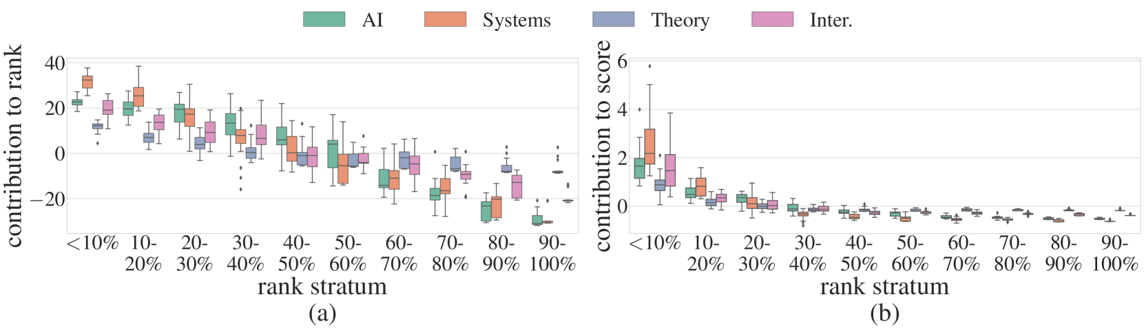
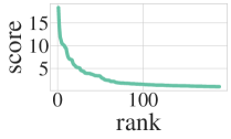
Figure 2: Feature contributions to rank and score for the CSRankings dataset, aggregated over 10% strata. In this ranking, 189 computer science departments are ranked based on a normalized publication count of the faculty across 4 research areas: AI (green), Systems (orange), Theory (purple), and Interdisciplinary (pink). (a) Systems is the most important feature for an item’s rank in the top-20%, followed by AI. AI becomes more important for the rest of the ranking strata.  (b) Feature contributions to score are less informative than to rank: both capture the same relative feature importance for the top 20%; however, feature contributions become small and very similar as more items are tied for their score. (See rank vs. score plot on the top-right.)

Example 1.

Consider a dataset $\mathcal{D}$ of college applicants in Figure 1, with scoring features $gpa$, $sat$, and $essay$. Very different scoring functions $f=0.4\times gpa+0.4\times sat+0.2\times essay$ and $g=1.0\times essay$ induce very similar rankings $r_{\mathcal{D},f}$ and $r_{\mathcal{D},g}$, with the same top-$4$ items appearing in the same order, apparently because $essay$ is the feature that is best able to discriminate between the top-$4$ and the rest, and — regardless of its weight — determines the relative order among the top-$4$.

This example shows that the weight of a scoring feature may not be indicative of its impact on the ranked outcome. Intuitively, this happens because rankings are, by definition, relative, while feature values, and scores computed from them, are absolute. That is, knowing the score of an item says little about the position of that item in the ranking relative to other items. The key insight then is that the impact of the scoring features on the ranking must be measured in a way that captures the lack of independence between per-item outcomes.

There has been substantial work on quantifying feature importance for classification (Covert et al. (2020); Datta et al. (2016); Guidotti et al. (2019); Lundberg and Lee (2017); Mohler et al. (2020); Ribeiro et al. (2016); Strumbelj and Kononenko (2010)), and one may be tempted to think that these methods can be reused to explain ranking. Unfortunately, this is not the case, because in classification, predictions are being made independently for each item. For example, in binary classification, if all points happen to fall on the positive side of the decision boundary, then all will receive the positive outcome. In contrast, in ranking, an outcome for some item v is not independent of the outcomes for items $\mathcal{D}\setminus\{\textbf{v}\}$. For example, only one item can occupy a specific rank position, and exactly $k$ items can appear at the top-$k$. This lack of independence has profound implications for how rankings are generated and explained.

Rankings have been treated differently from classification in predictive contexts, as evidenced by the rich literature on learning-to-rank (Li (2014)). Rankings have also been treated differently to quantify fairness (Zehlike et al. (2022a, b)). Similarly, interpretability methods have to be customized for rankings, as we do in this work. We use the Quantitative Input Influence (QII) framework by Datta et al. (2016) as the starting point and augment it with several Quantities of Interest (QoI) that are appropriate for ranking, including score, rank, pair-wise preference, and top-$k$. We preview two of these QoIs in Figure 2, showing that they surface different insights about feature importance.

Summary of approach and contributions.

We build on the Quantitative Input Influence (QII) framework by Datta et al. (2016) to quantify the influence of features on the ranked outcome. We use QII as the starting point because this framework flexibly and naturally accommodates local, group-wise, and global explanations. This flexibility is essential for expressing new quantities of interest for ranking, because of the need to accommodate the lack of independence between per-item outcomes, as already discussed.

QII produces explanations of the features based on Shapley values Shapley and others (1953). Shapley value is a canonical method of dividing revenue in cooperative games based on the expected payment. QII uses Shapley values to explain the influence of an item’s features (players) on the classification outcome for that item (cooperative game).

QII was proposed in the context of predictive classification, and extend it for ranking. Our first contribution is a formalization of several natural quantities of interest (QoI) that are appropriate for ranking, expressing feature contributions to an item’s score or rank, to its presence or absence at the top-$k$, and to the relative order between a pair of items.

QII has not been seeing much adoption because, unlike in the case of LIME Ribeiro et al. (2016) and SHAP Lundberg and Lee (2017), only a preliminary implementation of QII is publicly available. Our second contribution is a robust and extensible open-source ShaRP library that implements QII, making this powerful framework — including also its functionality for explaining classification outcomes — available to others in the community.

Ultimately, explanations are only useful if they help uncover important insights about the decision-making process. Our third contribution is an extensive experimental evaluation of Shapley-based explanations for ranking, in score-based and learning-to-rank settings. We present results with numerous synthetic datasets, showing that feature importance for all QoIs depends on the properties of the data distribution even when the scoring function remains fixed. Further, we show that the quantities of interest we define bring interesting — and complementary — insights about the data that cannot be captured simply by the relationship between the scores and the ranks. Finally, we conduct a qualitative evaluation of ShaRP for CSRankings — a real dataset that ranks 189 Computer Science departments in the US based on a normalized publication count of the faculty across 4 research areas: AI, Systems, Theory, and Interdisciplinary (Berger (2023)). Our results, previewed in Figure 2, show that ShaRP surfaces subtle and valuable insights about the importance of specific research areas. We observe that Systems is the most important feature for attaining a high rank, followed by AI.

2 Related work

We are aware of several other lines of work on interpretability in ranking. Yang et al. (2018) proposed a “nutritional label” for score-based rankers that includes two visual widgets that explain the ranking methodology and outcome: “Recipe” shows scoring feature weights and “Ingredients” shows the features (scoring or not) that have the strongest (global) Spearman’s rank correlation with the score. The authors observed that the weight of a feature in the “Recipe” rarely corresponds to how well it correlates with the score.

Gale and Marian (2020) developed “participation metrics” for score-based rankers that measure the contributions of scoring features to whether an item v is among the top-$k$. Their most important metric, “weighted participation,” attributes the fact that v is included among the top-$k$ to the values of its scoring features, the weight of these features in the scoring function, the distance of v’s feature values from the maximum possible values, and to whether these values exceed the $k^{th}$ highest values for each feature among all items in $\mathcal{D}$. Unlike this work, we use Shapley values to measure the average marginal contribution of a feature, aggregated over all feature subsets, weighted by subset size. Our QoI that is most similar to weighted participation is the top-$k$ QoI, which expresses the probability that intervening on a subset of features will land an item in the top-$k$, computed for all strata (not only for the items that are actually among the top-$k$).

Yuan and Dasgupta (2023) designed an interface for sensitivity analysis of ranked synthetic datasets using Shapley values. Their methods are designed specifically for linear weighted scoring functions with two Gaussian features, and compute feature contributions for custom quantiles of a ranking. They define ranking-specific quantities of interest. Our methods are more general and more flexible, accommodating a variety of feature distributions, real datasets, quantities of interest, and scoring functions.

Anahideh and Mohabbati-Kalejahi (2022) provide local explanations of feature importance in the immediate neighborhood of an item. They consider multiple methods including Shapley values, and conclude that it is the best method for local explanations. To apply Shapley values and calculate the local contributions using only the surrounding neighborhood, they fit a linear model and use a subset of the features per coalition. Like Anahideh and Mohabbati-Kalejahi (2022), we show that feature importance differs significantly per rank stratum. However, in contrast to the findings of Anahideh and Mohabbati-Kalejahi (2022), we find that slight changes in feature values can move an item significantly in the ranks, far beyond the local neighborhood (e.g., see Figure 7).

Finally, Hu et al. (2022) developed PrefSHAP, a method for explaining pairwise preference data from learned rankers. They calculate the Shapley value contributions for pairwise preferences on a new quantity they propose: They create artificial items from the pair of items simultaneously for each coalition, and then evaluate how the preference changes. While this quantity can be applied to any preferential function, they introduce PrefSHAP specifically for functions that use the generalized preferential kernel defined in Chau et al. (2022) for running time efficiency. They compare their results with an adaptation of SHAP for preference models and show that this adaptation does not capture the contributions properly. We work with score-based rankers, not learned pairwise preferences, but, also argue that ranking-specific quantities of interest are needed to explain rankings.

In summary, we share motivation with these lines of work, but take a leap, describing the first comprehensive Shapley-value-based framework for rankings and preferences.

3 Preliminaries and Notation

Ranking.

Let $\mathcal{A}$ denote an ordered collection of features (equiv. attributes), and let $\mathcal{D}_{\mathit{}}$ denote a set of items (equiv. points or candidates). An item $\textbf{v}=(v_{1},\dots,v_{d})\in\mathbb{R}^{d}$ assigns values to $|\mathcal{A}|=d$ features, and may additionally be associated with a score. Score-based rankers use a scoring function $f(\textbf{v})$ to compute the score of v. For example, using $f_{1}(\textbf{v})=0.4\times gpa+0.4\times sat+0.2\times essay$, we compute $f(\texttt{Bob})=4.6$ and $f(\texttt{Leo})=3.8$.

A ranking $r_{\mathcal{D}}$ is a permutation over the items in $\mathcal{D}_{\mathit{}}$. Letting $n=\left|\mathcal{D}_{\mathit{}}\right|$, we denote by $r_{\mathcal{D}}=\langle\textbf{v}_{1},\ldots,\textbf{v}_{n}\rangle$ a ranking that places item $\textbf{v}_{i}$ at rank $i$. We denote by $r_{\mathcal{D}}(i)$ the item at rank $i$, and by $r_{\mathcal{D}}^{-1}(\textbf{v})$ the rank of item v in $r_{\mathcal{D}}$. In score-based ranking, we are interested in rankings induced by some scoring function $f$. We denote these rankings $r_{\mathcal{D},f}$. For example, in Figure 1(b), $r_{\mathcal{D},f}(1)=\texttt{Bob}$, $r_{\mathcal{D},f}^{-1}(\texttt{Leo})=7$. We assume that $r_{\mathcal{D},f}^{-1}(\textbf{v}_{1})<r_{\mathcal{D},f}^{-1}(\textbf{v}_{2})<\dots<r_{\mathcal{D},f}^{-1}(\textbf{v}_{n})$, where a smaller rank means a better position in the ranking.

We are often interested in a sub-ranking of $r_{\mathcal{D},f}$ containing its best-ranked $k$ items, for some integer $k\leq n$; this sub-ranking is called the top-$k$. The top-$4$ of the ranking in Figure 1(b) is $\mathord{\langle\texttt{Bob},\texttt{Cal},\texttt{Dia},\texttt{Eli}\rangle}$.

Our goal is to explain the importance of features $\mathcal{A}$ to the ranking $r_{\mathcal{D},f}$. We will do so using Shapley values.

Shapley values and quantities of interest.

For a subset of features $\mathcal{S}\subseteq\mathcal{A}$, let $\textbf{v}_{\mathcal{S}}$ denote a projection of v onto $\mathcal{S}$. Continuing with the example in Figure 1, $(\texttt{Bob},\texttt{4},\texttt{5},\texttt{2})_{\{name,gpa\}}=(\texttt{Bob},\texttt{4})$. Let U $=\langle\textbf{u}_{1},\dots,\textbf{u}_{m}\rangle$ denote a vector of $m$ items, sampled from $\mathcal{D}$ using some sampling mechanism. For a subset of features $\mathcal{S}\in\mathcal{A}$, let $\textbf{v}_{\mathcal{A}\setminus\mathcal{S}}\textbf{U}_{\mathcal{S}}=\langle\textbf{v}_{\mathcal{A}\setminus\mathcal{S}}(\textbf{u}_{1})_{\mathcal{S}},\dots,\textbf{v}_{\mathcal{A}\setminus\mathcal{S}}(\textbf{u}_{m})_{\mathcal{S}}\rangle$ denote a vector of items in which each item $\textbf{v}_{\mathcal{A}\setminus\mathcal{S}}(\textbf{u}_{i})_{\mathcal{S}}$ takes on the values of the features in $\mathcal{S}$ from $\textbf{u}_{i}$, and the values of the remaining $\mathcal{A}\setminus\mathcal{S}$ features from v.

Algorithm 1 presents the computation of feature importance — in the form of a vector of Shapley values $\phi(\textbf{v})$ — to QoIs that can be specified for a single item v, independently of other items. The algorithm relies on black-box access to the model that generates the outcomes (i.e., specifying an input to the model and observing the output).

The algorithm takes as input a dataset $\mathcal{D}$, an item v for which the explanation is generated, the number of samples to draw $m$, and the QoI function $\iota()$ based on which we quantify the feature importance. Note that $m$ is user-defined and controls the quality of approximation. Passing in the full set of items $\mathcal{D}$ and setting $m=|\mathcal{D}-1|$ results in the exact computation of the Shapley values (i.e., the item v’s features are quantified against every other item in $\mathcal{D}$). Passing in $\mathcal{D}^{\prime}\subset\mathcal{D}$ that corresponds to a specific group (e.g., women) computes group-specific feature importance for the given QoI.

For every feature $i\in\mathcal{A}$, the algorithm computes every coalition of the remaining features $\mathcal{S}\subseteq\mathcal{A}\setminus\{i\}$. For each coalition $\mathcal{S}$, it draws $m$ samples from $\mathcal{D}$. Two vectors of items are created based on this sample: $\textbf{U}_{1}$, in which feature values of the coalition vary as in U and the remaining features are fixed to their values in v; and $\textbf{U}_{2}$, in which features in the coalition and the feature of interest $i$ vary as in U, and the remaining features are fixed to their values of v. The importance of the coalition, $\phi_{i_{\mathcal{S}}}(\textbf{v})$, is computed by invoking the function $\iota()$, which computes the difference in QoI between the two vectors of items $\textbf{U}_{1}$ and $\textbf{U}_{2}$. This value is added to the contribution of feature $i$, $\phi_{i}(\textbf{v})$ weighted by the number of coalitions of this size ${d-1\choose|S|}$, and the total number of possible coalition sizes $d$.

Algorithm 1 Feature importance for per-item outcomes

Input: Dataset $\mathcal{D}$, item v, number of samples $m$, $\iota()$
Output: Shapley values $\phi(\textbf{v})$ of v’s features

1:  $\phi(\textbf{v})=\langle 0,\ldots,0\rangle$

2:  for $i\in\mathcal{A}$ do

3:     for  $\mathcal{S}\subseteq\mathcal{A}\setminus\{i\}$ do

4:        $\textbf{U}\sim\mathcal{D}\setminus$v$,m$

5:        $\textbf{U}_{1}=\textbf{v}_{\mathcal{A}\setminus\mathcal{S}}\textbf{U}_{\mathcal{S}}$

6:        $\textbf{U}_{2}=\textbf{v}_{\mathcal{A}\setminus\{\mathcal{S}\cup i\}}\textbf{U}_{\mathcal{S}\cup i}$

7:        $\phi_{i_{\mathcal{S}}}(\textbf{v})=\iota(\textbf{U}_{1},\textbf{U}_{2})$

8:        $\phi_{i}(\textbf{v})=\phi_{i}(\textbf{v})+\frac{1}{d}\frac{1}{{d-1\choose|S|}}\phi_{i_{\mathcal{S}}}(\textbf{v})$

9:     end for

10:  end for

11:  return $\phi(\textbf{v})$

4 Quantities of Interest for Ranking

We use Algorithm 1 as a starting point for computing feature importance for ranked outcomes. We will define different QoIs with the help of the $\iota()$ function.

Score QoI.

Recall that $f$ denotes the scoring function. We overload notation and denote by $f(\textbf{U})$ the computation of the score for each item in U, and return these scores as a vector. Since $\textbf{U}_{1}$ and $\textbf{U}_{2}$ are vectors of items constructed from the same vector U, they are of the same size. To quantify feature importance to an item’s score, we define $\iota_{Score}$ as the mean of the (per-element) difference of $f(\textbf{U}_{1})$ and $f(\textbf{U}_{2})$:

$$\iota_{Score}(\textbf{U}_{1},\textbf{U}_{2},f)=\mathbb{E}\left[f(\textbf{U}_{1})-f(\textbf{U}_{2})\right]$$

This $\iota_{Score}$ is commonly used for Shapley value feature importance, and we use it as a qualitative baseline for comparison with the other QoIs we propose.

Rank QoI.

An item’s rank is computed with respect to all other items in the sample. For this reason, to quantify the impact of v’s features on its rank, we must compute the ranking of each intervened-upon instantiation of v in $\mathcal{D^{\prime}}$. This adds two steps to calculating this QoI compared to the score QoI. The item we are explaining needs to be removed from $\mathcal{D^{\prime}}$, and the score of each item $\textbf{u}_{i}\in\textbf{U}_{1}$ (and equivalently $\textbf{u}_{j}\in\textbf{U}_{2}$) needs to be compared to the scores of all items in $\mathcal{D^{\prime}}$.

Algorithm 2 $\iota_{Rank}$

Input: Dataset $\mathcal{D}$, scoring function $f$, item v, $\textbf{U}_{1}$, $\textbf{U}_{2}$, number of samples $m$
Output: $\phi$

1:  $\phi=0$

2:  for $i\in\{1,\dots,m\}$ do

3:     $\textbf{u}_{1}=\textbf{U}_{1}(i)$

4:     $\textbf{u}_{2}=\textbf{U}_{2}(i)$

5:     $\mathcal{D}_{1}=\mathcal{D}\setminus\{\textbf{v}\}\cup\{\textbf{u}_{1}\}$

6:     $\mathcal{D}_{2}=\mathcal{D}\setminus\{\textbf{v}\}\cup\{\textbf{u}_{2}\}$

7:     $\phi=\phi+r^{-1}_{\mathcal{D}_{2},f}(\textbf{u}_{2})-r^{-1}_{\mathcal{D}_{1},f}(\textbf{u}_{1})$

8:  end for

9:  return $\phi/|\textbf{U}_{1}|$

The computation of $\iota_{Rank}$ is summarized in Algorithm 2. We consider each a pair of corresponding (i.e., at the same position in their respective vector) samples $\textbf{u}_{1}\in\textbf{U}_{1}$ and $\textbf{u}_{2}\in\textbf{U}_{2}$, and compute $\mathcal{D}_{1}=\mathcal{D}\setminus\{\textbf{v}\}\cup\{\textbf{u}_{1}\}$ and $\mathcal{D}_{2}=\mathcal{D}\setminus\{\textbf{v}\}\cup\{\textbf{u}_{2}\}$. Next, we rank $\mathcal{D}_{1}$ and $\mathcal{D}_{2}$ on $f$, and compute the difference in ranks $r^{-1}_{\mathcal{D}_{2},f}(\textbf{u}_{2})-r^{-1}_{\mathcal{D}_{1},f}(\textbf{u}_{1})$. Note that we are subtracting the rank of $\textbf{u}_{1}$ from the rank of $\textbf{u}_{2}$, since a lower rank corresponds to a higher (better) position in the ranking. We return the average (expected) rank-difference as $\iota$.

Top-$k$ QoI.

To compute feature importance that explains whether an item appears at the top-$k$, for some given $k$, we use a similar method as for rank QoI. The difference is that, rather than computing the difference in rank positions for a given pair of items $\textbf{u}_{1}$ and $\textbf{u}_{2}$, we instead check whether one, both, or neither of them are at the top-$k$. As in Algorithm 2, we work with $\mathcal{D}_{1}=\mathcal{D}\setminus\{\textbf{v}\}\cup\{\textbf{u}_{1}\}$ and $\mathcal{D}_{2}=\mathcal{D}\setminus\{\textbf{v}\}\cup\{\textbf{u}_{2}\}$ for each sample. We increase the contribution to $\phi$ by 1 if only $\textbf{u}_{1}$ is in the top-$k$, and decrease it by 1 if only $\textbf{u}_{2}$ is in the top-$k$. We omit pseudocode due to space constraints.

Pairwise QoI.

We developed a method for computing feature importance for the relative order between a pair of items u and v, to answer the question of why u is ranked higher than v (i.e., $\textbf{u}\succ\textbf{v}$). In Algorithm 3, we create feature coalitions as in Algorithm 1 and then, instead of sampling from $\mathcal{D}$, we create $\textbf{U}_{1}$ and $\textbf{U}_{2}$ as vectors of 1 element each, based on the values of the items being compared. We then invoke the $\iota()$ function to compute the feature importance with respect to the difference in score, or rank, or the presence/absence at the top-$k$, as described earlier in this section.

Algorithm 3 Feature importance for preference $\textbf{u}\succ\textbf{v}$

Input: Item v, item u, $\iota()$
Output: Shapley values $\phi(\textbf{u}\succ\textbf{v})$ that explain why u is ranked higher than v

1:  $\phi(\textbf{u}\succ\textbf{v})=\langle 0,\ldots,0\rangle$

2:  for $i\in\mathcal{A}$ do

3:     for $\mathcal{S}\subseteq\mathcal{A}\setminus\{i\}$ do

4:        $\textbf{U}_{1}=\langle\textbf{v}_{\mathcal{A}\setminus\mathcal{S}}\textbf{u}_{\mathcal{S}}\rangle$

5:        $\textbf{U}_{2}=\langle\textbf{v}_{\mathcal{A}\setminus\{\mathcal{S}\cup i\}}\textbf{u}_{\mathcal{S}\cup i}\rangle$

6:        $\phi_{i_{\mathcal{S}}}(\textbf{u}\succ\textbf{v})=\iota(\textbf{U}_{1},\textbf{U}_{2})$

7:        $\phi_{i}(\textbf{u}\succ\textbf{v})=\phi_{i}(\textbf{u}\succ\textbf{v})+\frac{1}{d}\frac{1}{{d-1\choose|S|}}\phi_{i_{\mathcal{S}}}(\textbf{u}\succ\textbf{v})$

8:     end for

9:  end for

10:  return $\phi(\textbf{u}\succ\textbf{v})$

5 Experimental Evaluation

In this section, we showcase the versatility of the ShaRP framework for explaining rankings.

Datasets and rankers.

We present results for CS Rankings, a real dataset that ranks 189 Computer Science departments in the US based on a normalized publication count of the faculty across 4 research areas (Berger (2023)). We use the scoring formula provided by csrankings.org: a geometric mean of the adjusted counts per area, $f=\sqrt[27]{(AC_{AI}^{5}+1)(AC_{Sys}^{12}+1)(AC_{Th}^{3}+1)(AC_{Int}^{7}+1)}$.

We also generate synthetic datasets in which items have 2 features, $x_{1}$ and $x_{2}$, distributed according to the uniform, Gaussian, or Bernoulli distributions, with varying parameters. We experiment with both independent and correlated features. Each synthetic dataset consists of $2,000$ items. We use three linear scoring functions: $f_{1}=0.8\times x_{1}+0.2\times x_{2}$, $f_{2}=0.5\times x_{1}+0.5\times x_{2}$, and $f_{3}=0.2\times x_{1}+0.8\times x_{2}$. We sample $m=1,999$ for each QoI computation that requires sampling (all except pairwise QoI). For the top-$k$ QoI, we set $k=200$ (10% of the data).

Finally, we use a benchmark dataset of 2000 candidates who are applying for a position at a fictional moving company from  Yang et al. (2021), with an LGBM ranker, for our learning-to-rank experiment.

Visualizing feature importance.

We use three methods for visualizing experimental results. The first, used in Figures 4a and 4b, is a waterfall visualization that presents feature importance for a single item (as in Lundberg and Lee (2017)). The second visualization, used in Figures 2, 3a, 5, 6, and 7, is a box-and-whiskers plot that aggregates local feature importance across ranking strata, each covering 10% of the range. This visualization allows us to see both the median contribution of each feature to a stratum and the variance in that feature’s contribution across the items in the stratum. The third visualization, used in Figures 3c and 3d, is a bar graph that presents feature contributions for pairwise QoI.

5.1 Qualitative Analysis of CS Ranking

(a) Feature contribution to the top-$k$ QoI, for $k=10\%$. Systems is the most important feature, followed by Interdisciplinary and AI, while Theory is least important.

Institution	AI	Systems	Theory	Inter.	Rank
Georgia Tech	28.5	7.8	6.9	10.2	5
Stanford	36.7	5.4	13.3	11.5	6
UMich	30.4	9.0	9.3	5.9	7

(b) Feature values and rank of three highly ranked departments: Georgia Tech, Stanford, and UMich.

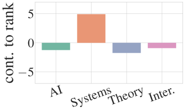
(c) Pairwise QoI explaining that Georgia Tech ranks higher than Stanford because of its relative strength in Systems.

(d) Pairwise QoI explaining that Stanford ranks higher than UMich despite Stanford’s relative weakness in Systems.

Figure 3: Feature importance for the top-$k$ QoI for CS Rankings, with further analysis of 3 departments using Pairwise QoI.

We already previewed the compelling results of Figure 2 in the Introduction. In that figure, we show feature contributions to rank and score QoI for the CS Rankings dataset, aggregated over 10% strata. According to rank QoI in Figure 2(a), Systems is the most important feature in all strata, followed closely by AI. Both features have the most positive contributions in the top strata and the most negative in the bottom strata. Further, we observe that feature contributions to score are less informative than to rank: both capture the same relative feature importance for the top 20%; however, feature contributions become small and very similar as more items are tied or nearly-tied for their scores, making it nearly impossible to quantify feature importance across strata.

Figure 3a presents the top-$k$ QoI for this dataset. The feature importance it shows is consistent with Figure 2(a) (score QoI), but the high positive impact of Systems on an department’s presence at the top-$k$ is even stronger pronounced. Additionally, unlike the score QoI, this top-$k$ QoI shows that Theory is impactful for getting into the top-$k$. Further, both top-$k$ and rank QoIs show that Systems and AI swap places in terms of importance, while score QoI does not detect this.

In Figure 3(b)-(d), we continue our analysis of the top-$k$ and consider the relative ranking of three universities: Georgia Tech in rank 5, Stanford in rank 6, and UMich in rank 7. We wish to understand why Georgia Tech is ranked higher than Stanford (Figure 3c), and why Stanford is ranked higher than UMich (Figure 3d). In both cases, Georgia Tech and UMich have lower values for all features except Systems. The Systems value of Georgia Tech is high enough to overcome the contributions of other features and rank it higher than Stanford. However, for UMich, we see that, while Systems is the most important feature in the top-10% stratum, it is not important enough to move UMich above Stanford. Note that adding the contributions for each feature adds up to the total difference in rank between each pair.

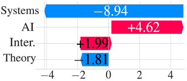
(a) South Carolina, ranked 101

(b) Wayne State, ranked 102

Figure 4: Feature contributions to rank QoI for two departments.

In Figure 4, we present the rank QoI for The University of South Carolina (rank 101) and Wayne State University (rank 102), using the waterfall visualization. These universities are ranked consecutively, but for different reasons. For South Carolina, Systems and Theory have negative contributions, while AI and Interdisciplinary have positive contribution. For Wayne State, only AI has a positive contribution, while other features have negative contributions.

5.2 Score-based Ranking with Synthetic Data

Figure 5: The rank QoI using $f_{2}=0.5\times x_{1}+0.5\times x_{2}$ for four datasets; $D_{1}$: $x_{1}\sim N(0.5,0.1)$, $x_{2}\sim Bern(0.5)$; $D_{2}$: $x_{1}\sim[0,1]$, $x_{2}\sim N(0.5,0.1)$; $D_{3}$: $x_{1}\sim[0,1]$, $x_{2}\sim[0,1]$; $D_{4}$: $x_{1}\sim N(0.5,0.05)$, $x_{2}\sim N(0.75,0.016)$, with -0.8 correlation. Feature contributions are different per rank stratum and data distribution.

Fixed scoring function, varying data distribution.

In this experiment, we illustrate that feature importance is impacted by the data distribution of the scoring features to a much greater extent than by the feature weights in the scoring function. Further, we show that feature importance varies by rank stratum. In Figure 5, we show rank QoI for 4 synthetic datasets, using the same scoring function, $f_{2}$.

We observe that, while the features have equal scoring function weights, their contributions to rank QoI differ for most datasets. In $D_{1}$, the Bernoulli-distributed $x_{2}$ determines whether the item is in the top or the bottom half of the ranking, while the Gaussian-distributed $x_{1}$ is responsible for the ranking inside each half. For $D_{2}$, the uniform $x_{1}$ has higher importance because it often takes on larger values than the Gaussian $x_{2}$. In $D_{4}$, $x_{1}$ and $x_{2}$ are negatively correlated, so when one contributes positively, the other contributes negatively. Only for $D_{3}$, with two uniform identically distributed features, the median contributions of both features are approximately the same within each stratum.

Additionally, we see that feature contributions differ per rank stratum. For example, for $D_{3}$, the medians show a downward trajectory across strata. This is because they quantify the expected change (positive or negative) in the number of rank positions to which the current feature values contribute. Also for $D_{3}$, feature contributions have higher variance in the middle of the range, because a 40-60% rank corresponds to many combinations of feature values.

Fixed data distribution, varying scoring function.

In this experiment, we investigate the impact of the scoring function on rank and top-$k$ QoI for two datasets. In Figure 6, we use $D_{3}$ and see that the contributions to rank QoI vary depending on the scoring function. For $f_{1}$, $x_{1}$ is the only important feature (although it carries 0.8 — and not 1.0 — of the weight). This can be explained by the compounding effect of the higher scoring function weight and higher variance of the distribution from which $x_{1}$ is drawn. Between $f_{2}$ and $f_{3}$, features $x_{1}$ and $x_{2}$ switch positions in terms of importance, and show a similar trend, despite being associated with different scoring function weights (0.5 & 0.5 vs. 0.2 & 0.8). This, again, can be explained by the higher variance of $x_{1}$, hence, $x_{2}$ needs a higher scoring function weight to compensate for lower variance and achieve similar importance.

Figure 6: Rank QoI for $D_{5}$: $x_{1}\sim N(0.5,0.1)$, $x_{2}\sim N(0.5,0.05)$. Subplots correspond to different scoring functions: $f_{1}=0.8\times x_{1}+0.2\times x_{2}$ (top), $f_{2}=0.5\times x_{1}+0.5\times x_{2}$ (middle), $f_{3}=0.2\times x_{1}+0.8\times x_{2}$ (bottom).

Figure 7: Top-$k$ QoI for $k=10\%$ and $D_{3}$: $x_{1}\sim[0,1]$, $x_{2}\sim[0,1]$. Subplots correspond to different scoring functions: $f_{1}=0.8\times x_{1}+0.2\times x_{2}$ (top), $f_{2}=0.5\times x_{1}+0.5\times x_{2}$ (bottom).

Access to the top-$k$ is determined by the interaction between the scoring feature weights and the distributions of these features. The higher the weight of the less important feature, the higher the likelihood for an item to move to the top-$k$ by changing the other feature. Figure 7 illustrates this for dataset $D_{3}$. Under $f_{1}$, items in the lower strata have a non-zero probability to move to the top-$k$ by changing the second feature, as indicated by the variance. In contrast, under $f_{2}$, with equal scoring feature weights, items in the bottom strata cannot change either feature sufficiently to move into the top-$k$, while items in the middle strata have a higher probability of moving to the top-$k$ compared to $f_{1}$, by changing either feature. Evidence that items from lower strata can move to the top-$k$ under some scoring functions and feature distributions counters the assumption of Anahideh and Mohabbati-Kalejahi (2022) that changes in rank are localized.

5.3 Learning-to-rank

In our final set of experiments, we showcase the use of ShaRPin a learning-to-rank (LtR) setting. For this, we use a benchmark dataset of 2000 candidates who are applying for a position at a fictional moving company from  Yang et al. (2021). The dataset contains three features: gender, qualification score (i.e., weight lifting ability) and race, along with the final score $Y$. The score $Y$ is computed by causal model $\mathcal{M}_{1}$ and used to rank the job applicants. The score $Y$ is then withheld, and an LGBM Ranker (Ke et al. (2017)) with the LambdaRank objective (Burges et al. (2006)) is trained on 80% of the data, with 20% reserved for testing.

Figure 8 shows the rank QoI for the test dataset, under two conditions. In Figure 8a, we show the rank QoI for a test set, using an LtR model trained on a dataset in which both race and, to some extent, gender, impact the final ranking, in addition to the qualification score. In Figure 8b, we show feature importance for a test set, but with an LtR model that is trained on a counterfactually fair data (per Yang et al. (2021)), in which the impact of race is reduced. Observe that the impact of the race feature is also lower in Figure 8b (after intervention) compared to Figure 8a (before intervention), as expected. Furthermore, the impact of the qualification feature is higher in Figure 8b, as expected, since the importance of race is now reduced.

(a) Qualification is the most important feature, but gender and race also impact the rank.

(b) Feature importance of race is lower when learning-to-rank model is trained on counterfactually fair data.

Figure 8: Rank QoI for two versions of the moving company hiring task from Yang et al. (2021), with learning-to-rank. Qualification is the most important feature, but gender and race also impact the rank. Feature importance differs across strata in both experiments.

6 Conclusions, Limitations, and Future Work

In this paper, we presented ShaRP, a comprehensive framework for quantifying feature importance for rankings. We used the Quantitative Influence (QII) framework as a starting point, and augmented it with several natural quantities of interest that can be used to explain the contributions of features to an item’s score or rank, to the relative order between a pair of items, and to the presence or absence of an item at the top-$k$. We implemented ShaRP in a software library, which we will contribute to the open source following publication.

We showcased the usefulness of ShaRP for qualitative analysis of an impactful real dataset and task — the ranking of Computer Science departments. We augmented this analysis with a thorough evaluation of our methods on numerous synthetic datasets, showing that the quantities of interest we define bring interesting — and complementary — insights about the data that cannot be captured simply by the relationship between the scores and the ranks. We showed that feature importance depends on the properties of the data distribution even if the scoring function remains fixed, and, further, that feature importance exhibits locality: it changes substantially depending on where in the ranking one looks.

Limitations and future work.

The most important limitation is that our evaluation of the usefulness of explainability methods did not include a user study. Understanding how humans make sense of feature importance in ranking and act on their understanding, is in our immediate plans.

An important technical limitation, which we share with QII, is that we require black-box access to the ranker. Recently, methods have been proposed to fit a ranker to the data and treat it as a surrogate black-box model. Developing methods for learning low-complexity black-box models is part of our future work. We also plan to support additional quantities of interest, accommodate a broader class of preferences in addition to ranking (e.g., partial orders), and develop a comprehensive benchmark that compares feature importance methods for rankings in terms of their usability, expressiveness, and performance.