Variable-Length Feedback Codes
over Known and Unknown Channels
with Non-vanishing Error Probabilities

Abstract

We study variable-length feedback (VLF) codes with noiseless feedback for discrete memoryless channels. We present a novel non-asymptotic bound, which analyzes the average error probability and average decoding time of our modified Yamamoto–Itoh scheme. We then optimize the parameters of our code in the asymptotic regime where the average error probability $\epsilon$ remains a constant as the average decoding time $N$ approaches infinity. Our second-order achievability bound is an improvement of Polyanskiy et al.’s (2011) achievability bound. We also universalize our code by employing the empirical mutual information in our decoding metric and derive a second-order achievability bound for universal VLF codes. Our results for both VLF and universal VLF codes are extended to the additive white Gaussian noise channel with an average power constraint. The former yields an improvement over Truong and Tan’s (2017) achievability bound. The proof of our results for universal VLF codes uses a refined version of the method of types and an asymptotic expansion from the nonlinear renewal theory literature.

I Introduction

Feedback does not increase the capacity of memoryless channels [1]. Yet, it simplifies the coding schemes that achieve the capacity [2, 3]. For fixed-length codes, Wagner et al. [4] show that feedback improves the second-order achievable rate for discrete memoryless channels (DMCs) that have multiple capacity-achieving input distributions with distinct dispersions.

The benefits of feedback are even more significant for variable-length feedback (VLF) codes, where the transmission stops at a random time depending on the noise realization. In his seminal work, Burnashev [5] shows that the optimal error exponent (also known as the reliability function) for VLF codes over a DMC is given by

$$E(R)=\lim_{\epsilon\to 0}-\frac{1}{\mathbb{E}\left[\tau\right]}\log\epsilon=C_{1}\left(1-\frac{R}{C}\right),$$ (1)

where $C$ is the capacity of the DMC, $C_{1}$ is the maximum Kullback–Leibler (KL) divergence between two conditional output distributions, $R\in(0,C)$ is the rate, $\epsilon$ is the error probability, and $\mathbb{E}\left[\tau\right]$ is the average decoding time of the code. For any $R<C$, the error exponent in (1) is larger than that for fixed-length codes without feedback [6]. To achieve the optimal error exponent, Burnashev proposes a two-phase coding scheme, where in the communication phase, the transmitter aims to increase the posterior of the transmitted message. If the largest posterior exceeds a threshold, the system goes into the confirmation phase, where the decoder tries to verify the correctness of the estimate in the confirmation phase.

Yamamoto and Itoh [7] propose an alternative scheme that achieves the optimal error exponent in (1). Yamamoto and Itoh’s scheme alternates between the communication and confirmation phases, each having fixed lengths, until a decision is made by the receiver. Any capacity-achieving fixed-length code can be used for the communication phase of the Yamamoto–Itoh scheme. In the confirmation phase, the transmitter transmits one of two control sequences, $(x_{\mathrm{A}},\dots,x_{\mathrm{A}})$ and $(x_{\mathrm{R}},\dots,x_{\mathrm{R}})$, where the first sequence indicates that the receiver should “accept” its current estimate, and the second sequence indicates that the receiver should “reject” its current estimate and start a new communication phase. The symbols $x_{\mathrm{A}}$ and $x_{\mathrm{R}}$ are chosen to be the two most distinguishable symbols in the sense that they achieve $C_{1}$. The receiver then constructs a (fixed-length) binary hypothesis test on the noisy versions of the control sequences and feeds its decision back to the transmitter. In [8], Chen et al. derive a non-asymptotic achievability bound for VLF codes with finite number of feedback instances; their code is a variant of Yamamoto–Itoh scheme where the length of each communication and confirmation phase may be distinct.

Although error exponent analysis elucidates how fast the error probability decays as the average decoding time $N\triangleq\mathbb{E}\left[\tau\right]$ grows to infinity, it does not explain the fundamental limit for a fixed error probability $\epsilon\in(0,1)$ and a finite $N$ of our interest. To address this issue, Polyanskiy et al. [9] extend Burnashev’s work to the regime with non-vanishing error probabilities and derive achievability and converse bounds on the logarithm of the maximum achievable codebook size $\log M^{*}(N,\epsilon)$ given an average decoding time $N$ and average error probability $\epsilon\in(0,1)$. They show

$$\frac{NC}{1-\epsilon}-\log N+O(1)\leq\log M^{*}(N,\epsilon)\leq\frac{NC}{1-\epsilon}+\frac{h_{\mathrm{b}}(\epsilon)}{1-\epsilon},$$ (2)

where $h_{\mathrm{b}}(\epsilon)\triangleq-\epsilon\log\epsilon-(1-\epsilon)\log(1-\epsilon)$ is the binary entropy function. This result implies that the $\epsilon$-capacity is $\frac{C}{1-\epsilon}$, and the second-order term in the achievable rate is $O\left(\frac{\log N}{N}\right)$. To achieve the lower bound in (2), they employ stop-feedback, which is a single bit of feedback that tells the transmitter whether to stop the transmission or to continue to transmit symbols. Polyanskiy et al.’s scheme uses a stop-at-time-zero strategy, which decodes to an arbitrary message at time zero with probability $\epsilon_{0}<\epsilon$, and with probability $1-\epsilon_{0}$, the scheme employs a code with an information-density threshold rule. Variants of Polyanskiy et al.’s coding scheme with a finite number of feedback instances include [10, 11, 12, 13, 14, 15]. Some of the extensions of [9] to multi-transmitter networks are [14, 16]. In [17], for symmetric binary-input channels, Naghshvar et al. develop a deterministic, one-phase coding scheme that achieves the optimal error exponent in (1). Their code has a novel encoder called the small-enough-difference (SED) encoder, which partitions the message set into two subsets at each time instance so that the probability difference between the two subsets is small enough. In [18, Remark 4], Naghshvar et al. extend their work to arbitrary DMCs by introducing the maximum extrinsic Jensen-Shannon encoder and derive a non-asymptotic bound for their code. In [19], Yang et al. extend Naghshvar et al.’s SED encoder to binary asymmetric channels (BACs) (i.e., channels with binary input and binary output), and derive refined non-asymptotic achievability bounds for the BAC and the binary symmetric channel (BSC).

Since the exact channel statistics are not always available to the code designer, it is desirable to construct universal codes in the sense that the DMC in use is known to belong a certain family of DMCs (e.g., DMCs with known input and output alphabet sizes, BSCs with unknown flip probability), but the exact channel transition kernel $P_{Y|X}$ is unknown to both the transmitter and receiver. Naturally, we desire the performance of the universal code to be as close as to that of the non-universal code (e.g., the capacity, the error exponent). In [20], Goppa proposes to use the maximum (empirical) mutual information (MMI) decoder, which decodes to the message whose codeword has the maximum empirical mutual information with the received output sequence. Goppa shows that for DMCs, the MMI decoder attains capacity universally. In [21, Th. 10.2], Csiszár and Körner show that the random coding error exponent for constant-composition codes is achieved universally by the MMI decoder. Universal channel coding is related to mismatched decoding, in which the decoder is fixed and potentially sub-optimal, and the goal is to optimize the codebook since both mismatched decoding and universal coding attempt to address channel uncertainty (see [22] for a review of mismatched decoding). Merhav [23] unifies the mismatched decoding and universal coding approaches, where he shows that for a given random coding distribution and a given class of metric decoders, their proposed generic universal decoder whose error probability is within a subexponential multiplicator factor of the best decoder in that class of decoders. Extensions of [21, Th. 10.2] to the Gaussian channel with an unknown deterministic interference signal and to the Gaussian intersymbol interference channel appear in [24] and [25], respectively. In [26], Tchamkerten and Telatar define universal VLF (UVLF) codes and show that Burnashev’s error exponent is universally achieved over a family of BSCs with an unknown flip probability $p<\frac{1}{2}$ and over a family of Z channels with unknown parameters. In [27, Th. 3], Lomnitz and Feder show that for DMCs, the empirical mutual information between input and output sequences is achievable universally in the VLF setting, which extends Goppa’s result to VLF codes. In [27, Th. 4], they also show that for arbitrary continuous channels with an average power constraint, the rate $R=-\frac{1}{2}\log(1-\hat{\rho}_{X^{n}Y^{n}}^{2})$ is universally achievable in the VLF setting, where $\hat{\rho}_{X^{n}Y^{n}}^{2}$ is the empirical correlation correlation between input $X^{n}$ and output $Y^{n}$. The quantity $-\frac{1}{2}\log(1-\rho^{2})$ is the mutual information of two Gaussian random variables with the correlation coefficient $\rho$. In [28], Merhav and Feder study the error exponents of universal decoding with an erasure option, where the trade-off between the probability of undetected error and the probability of erasure is considered; this problem is related to UVLF codes in the sense that at each time, the UVLF decoder chooses between decoding to the “erasure” option and a message.

I-A Our Main Contributions

In this paper, we study VLF and UVLF codes in the regime that the error probability $\epsilon\in(0,1)$ is non-vanishing. For an arbitrary DMC with $C_{1}<\infty$, equivalently, all entries of the channel transition kernel $P_{Y|X}$ are positive, we improve the second-order term in the lower bound in (2) for VLF codes from $-\log N$ to $-\frac{C}{C_{1}}\log N$. Our proposed VLF code is a modified Yamamoto–Itoh scheme with two communication and one confirmation phases, where each phase has a random stopping time, similar to the code in [26]. In Theorem 1, we derive a novel non-asymptotic achievability bound; in Theorem 2, we analyze the non-asymptotic bound to derive the asymptotic bound with the improved second-order term. For UVLF codes, we assume that a training sequence of length $\ell$ is available prior to the communication. In Theorem 3, for UVLF codes, we derive an asymptotic achievability bound for an arbitrary DMC with $C_{1}<\infty$, where the second order term is $-\frac{C}{C_{1}}\log N-\min\left\{\frac{|\mathcal{X}||\mathcal{Y}|}{2},\left(|\mathcal{X}|-\frac{3}{2}\right)\left(|\mathcal{Y}|-\frac{3}{2}\right)+\frac{3}{4}\right\}\log N$. Our UVLF code universalizes the Yamamoto–Itoh scheme by replacing the information-density threshold rule in the communication phases with the empirical mutual information threshold rule. This empirical mutual information threshold rule is also used in [26]. Unlike [26], during the second communication phase, we do not discard the symbols from the first communication phase, which is essential for the derivation of Theorem 3. We use the training sequence only in the confirmation phase of the scheme, where we construct a sequential hypothesis test for the “accept” and “reject” hypotheses. In the proof of Theorem 3, we use the result in [29, Th. 4.5] from the nonlinear renewal theory literature to bound the expected stopping time associated associated with the empirical mutual information. We also use the refined method of types from [30] to get a tight tail probability bound for the empirical mutual information evaluated on a joint type formed from two independent sequences.

Theorems 4 and 5 extend our achievability bounds for VLF and UVLF codes to the Gaussian channel with an average power constraint. For UVLF codes for the Gaussian channel, we consider the scenario where the noise variance $\sigma_{0}^{2}$ of the channel is unknown to the transmitter and the receiver. Note that this model is equivalent to slow fading channel with a fixed an unknown fading factor and a known noise variance. For this problem, as our universal decoding metric, we employ the mutual information associated with the maximum likelihood estimator of the input-output pair $(X^{n},Y^{n})$ within the class of jointly Gaussian distributions with zero mean, which equals $-\frac{1}{2}\log(1-\hat{\rho}^{2}_{X^{n}Y^{n}})$, where $\hat{\rho}^{2}_{X^{n}Y^{n}}$ is the empirical correlation coefficient between $X^{n}$ and $Y^{n}$. This universal decoding metric is also used in [27]; a similar universal metric that also depends on the Gaussian input distribution is proposed in [23, Example 2]. Our results here refine the achievability results of Lomnitz and Feder [27, Th. 4].

I-B Paper Organization

The organization of the paper is as follows. Section II defines the notation, Section III formulates the problems, Section IV presents our main results, Section V extends our results to the Gaussian channel, and Sections VI–VIII contain the proofs. Section IX concludes the paper.

II Notation and Definitions

For $n\in\mathbb{N}$, we denote $[n]\triangleq\{1,\dots,n\}$ and the length-$n$ vector $x^{n}\triangleq(x_{1},\dots,x_{n})$. The distribution of a random variable $X$ on an alphabet $\mathcal{X}$ is denoted by $P_{X}$. For any random variable $X$, we define the constant $b(X)=\min\big{\{}\frac{\mathbb{E}\left[(X^{+})^{2}\right]}{\mathbb{E}\left[X\right]},\mathrm{ess}\sup(X)\big{\}}$, which is an upper bound on the expected stopping time associated with the random walk $\{\sum_{i=1}^{n}X_{i},n\geq 1\}$, where $X,X_{1},X_{2},\dots$ are independent and identically distributed (i.i.d.). The set of all distributions on $\mathcal{X}$ is denoted by $\mathcal{P}(\mathcal{X})$. The Gaussian random vector with mean $\bm{\mu}$ and covariance matrix $\mathsf{\Sigma}$ is denoted by $\mathcal{N}(\bm{\mu},\mathsf{\Sigma})$.

A DMC is defined by the single-letter channel transition kernel $P_{Y|X}\colon\mathcal{X}\to\mathcal{Y}$, where $\mathcal{X}$ and $\mathcal{Y}$ are the input and output alphabets. The DMC acts on each input symbol independently of others, i.e., $P_{Y^{n}|X^{n}}(y^{n}|x^{n})=\prod_{i=1}^{n}P_{Y|X}(y_{i}|x_{i})$ for all $x^{n}\in\mathcal{X}^{n}$ and $y^{n}\in\mathcal{Y}^{n}$. The set of all DMCs with input alphabet $\mathcal{X}$ and output alphabet $\mathcal{Y}$ is denoted by $\mathcal{P}(\mathcal{Y}|\mathcal{X})$.

All logarithms have base $e$. The information density is

$$\imath(x;y)\triangleq\log\frac{P_{Y|X}(y|x)}{P_{Y}(y)},$$ (3)

where the output distribution $P_{Y}$ is induced by a fixed input distribution $P_{X}$ and the DMC $P_{Y|X}$ (the dependence of the information density on $(P_{X},P_{Y|X})$ is suppressed). The mutual information associated with $P_{X}$ and $P_{Y|X}$ is denoted as

$$I(P_{X},P_{Y|X})\triangleq\sum_{x\in\mathcal{X},y\in\mathcal{Y}}P_{XY}(x,y)\log\frac{P_{Y|X}(y|x)}{P_{Y}(y)}.$$ (4)

The capacity of a DMC $P_{Y|X}$ is

$$C\triangleq\max\limits_{P_{X}\in\mathcal{P}(\mathcal{X})}I(P_{X},P_{Y|X}).$$ (5)

The entropy of $P_{X}$ is denoted by $H(P_{X})$, and the KL divergence between $P_{X}$ and $Q_{X}$ on the same alphabet $\mathcal{X}$ is denoted by $D(P_{X}\|Q_{X})$. The error exponent (1) achieved at zero rate is defined as

$$C_{1}\triangleq\max_{(x,x^{\prime})\in\mathcal{X}^{2}}D(P_{Y|X=x}\|P_{Y|X=x^{\prime}}).$$ (6)

The empirical distribution (or type) of a sequence $x^{n}\in\mathcal{X}^{n}$ is defined as

$$\hat{P}_{x^{n}}(x)\triangleq\frac{1}{n}\sum_{i=1}^{n}1\{x_{i}=x\},\quad x\in\mathcal{X}.$$ (7)

The conditional type of a sequence $(x^{n},y^{n})\in\mathcal{X}^{n}\times\mathcal{Y}^{n}$ is defined similarly to (7) and is denoted by $\hat{P}_{y^{n}|x^{n}}(y|x)$. The empirical mutual information associated with sequences $(x^{n},y^{n})$ is denoted by $I(\hat{P}_{x^{n}},\hat{P}_{y^{n}|x^{n}})$. The set of length-$n$ types on an alphabet $\mathcal{X}$ is denoted by $\mathcal{P}_{n}(\mathcal{X})\triangleq\{P_{X}\in\mathcal{P}(X)\colon nP_{X}(x)\in\mathbb{Z}\,\,\forall\,x\in\mathcal{X}\}.$ The type class of $P_{X}$ is defined as $\mathcal{T}_{n}(P_{X})\triangleq\{x^{n}\in\mathcal{X}^{n}\colon\hat{P}_{x^{n}}=P_{X}\}$.

We use the standard $o(\cdot)$, $O(\cdot)$, and $\Omega(\cdot)$ notations.

III Problem Formulation

We here formalize VLF and UVLF codes.

Definition 1 ([9, Def. 1])

Fix $\epsilon\in(0,1)$, $N>0$, and a positive integer $M$. An $(N,M,\epsilon)$-VLF code comprises

1. a common randomness random variable $U$ that has a finite alphabet $\mathcal{U}$ and an associated probability distribution $P_{U}$, (The realization $u$ of $U$ is revealed to the transmitter and receiver before the start of transmission to initialize the codebook.)

2. encoding functions $\mathsf{f}_{t}\colon\mathcal{U}\times[M]\times\mathcal{Y}^{t-1}\times\mathcal{P}(\mathcal{Y}|\mathcal{X})\to\mathcal{X}$ such that

   $$X_{t}=\mathsf{f}_{t}(U,W,Y^{t-1},P_{Y|X})\quad\forall t\in\mathbb{N},$$ (8)

3. a random stopping time $\tau\in\mathbb{N}$ of the filtration generated by $\{U,Y^{t}\}_{t=0}^{\infty}$, which satisfies the average decoding time constraint

   $$\mathbb{E}\left[\tau\right]\leq N,$$ (9)

4. a decoding function $\mathsf{g}_{\mathcal{\tau}}\colon\mathcal{U}\times\mathcal{Y}^{\tau}\times\mathcal{P}(\mathcal{Y}|\mathcal{X})\to[M]$ such that

   $$\hat{W}=\mathsf{g}_{\tau}(U,Y^{\tau},P_{Y|X}),$$ (10)

   where $\hat{W}$ is the estimate of the equiprobable message $W$, and the average error probability does not exceed $\epsilon$, i.e.,

   $$\mathbb{P}\left[\hat{W}\neq W\right]\leq\epsilon.$$ (11)

Definition 2

Let $\{(x_{i},\bar{Y}_{i})\}_{i=1}^{\ell}$ be a training sequence available to the transmitter and the receiver prior to the communication, where each $x\in\mathcal{X}$ appears at least $\lfloor\frac{\ell}{|\mathcal{X}|}\rfloor$ times in $x^{\ell}$, and $\bar{Y}^{\ell}\sim P_{Y^{\ell}|X^{\ell}=x^{\ell}}$. An $(N,M,\epsilon,\ell)$-UVLF code is defined similarly to an $(N,M,\epsilon)$-VLF code except that the encoding functions $\{\mathsf{f}_{t}\}_{t=1}^{\infty}$ and the decoding function $\mathsf{g}_{\tau}$ can depend on the training sequence $\{(x_{i},\bar{Y}_{i})\}_{i=1}^{\ell}$ and the input and output alphabet sizes $|\mathcal{X}|$ and $|\mathcal{Y}|$ but not on the channel transition kernel $P_{Y|X}$. We do not count the training sequence length $\ell$ towards the decoding time.

We define the maximum achievable codebook sizes $M^{*}(N,\epsilon)$ and $M_{\mathrm{U}}^{*}(N,\epsilon)_{\mathrm{UVLF}}$ as

$$M^{*}(N,\epsilon) \triangleq\max\{M\in\mathbb{N}\colon\,\exists\,(N,M,\epsilon)\text{-VLF code}\}$$ (12)

$$M_{\mathrm{U}}^{*}(N,\epsilon,\ell) \triangleq\max\{M\in\mathbb{N}\colon\exists\,(N,M,\epsilon,\ell)\text{-UVLF code}\}.$$ (13)

IV Main Result

Our first result is a non-asymptotic achievability bound for VLF codes, where the channel transition kernel $P_{Y|X}$ is known.

Theorem 1

Fix a positive integer $M$, positive constants $\gamma_{1}<\gamma_{2}$, $a_{\mathrm{A}}$, and $a_{\mathrm{R}}$, $\epsilon_{0}\in(0,1)$, and a capacity-achieving input distribution $P_{X}$. Define

$$(x_{\mathrm{A}},x_{\mathrm{R}})\triangleq\operatorname*{arg\,max}_{(x,x^{\prime})\in\mathcal{X}^{2}}D(P_{Y|X=x}\|P_{Y|X=x^{\prime}}).$$ (14)

There exists an $(N,M,\epsilon)$-VLF code with

$$N \leq(1-\epsilon_{0})N^{\prime}$$ (15)

$$\epsilon \leq\epsilon_{0}+(1-\epsilon_{0})\epsilon^{\prime},$$ (16)

where

$$\epsilon^{\prime} =(M-1)\left(\exp\{-(\gamma_{1}+a_{\mathrm{A}})\}+\exp\{-\gamma_{2}\}\right)$$ (17)

$$N^{\prime} =\frac{\gamma_{1}+b}{C}$$

$$+((M-1)\exp\{-\gamma_{1}\}+\exp\{-a_{\mathrm{R}}\})\frac{\gamma_{2}-\gamma_{1}+b}{C}$$

$$+\frac{a_{\mathrm{A}}+b_{\mathrm{A}}}{D(P_{Y|X=x_{\mathrm{A}}}\|P_{Y|X=x_{\mathrm{R}}})}$$

$$+(M-1)\exp\{-\gamma_{1}\}\frac{a_{\mathrm{R}}+b_{\mathrm{R}}}{D(P_{Y|X=x_{\mathrm{R}}}\|P_{Y|X=x_{\mathrm{A}}})}$$ (18)

$$b =b(\imath(X;Y)),\quad b_{\mathrm{A}}=b\left(\log\frac{P_{Y|X=x_{\mathrm{A}}}(Y_{\mathrm{A}})}{P_{Y|X=x_{\mathrm{R}}}(Y_{\mathrm{A}})}\right),$$ (19)

$$b_{\mathrm{R}} =b\left(\log\frac{P_{Y|X=x_{\mathrm{R}}}(Y_{\mathrm{R}})}{P_{Y|X=x_{\mathrm{A}}}(Y_{\mathrm{R}})}\right),$$ (20)

$(X,Y)\sim P_{X}P_{Y|X}$, $Y_{\mathrm{A}}\sim P_{Y|X=x_{\mathrm{A}}}$, and $Y_{\mathrm{R}}\sim P_{Y|X=x_{\mathrm{R}}}$.

The proposed coding scheme to prove Theorem 1 is a variant of the Yamamoto–Itoh scheme [7] and is modified from Telatar and Tchamkerten’s VLF coding scheme [26], which is designed for unknown channels. Our code is similar to the code in [8] in limiting the number of phases to a finite integer, but differs from it as each phase in our code has a random stopping time. Our code has two communication phases (C1 and C2) and one confirmation phase (HT), where the HT phase is between the C1 and C2 phases. We combine the Yamamoto–Itoh scheme with the stop-at-time-zero strategy used in [9], in which the code stops and decodes to an arbitrary message at time zero with probability $\epsilon_{0}$ and employs the Yamamoto–Itoh scheme with probability $1-\epsilon_{0}$. Decoding occurs either at time zero, or at the end of the HT phase, or at the end of the C2 phase. At large average decoding times $N$, the stop-at-time-zero strategy with a non-zero $\epsilon_{0}$ improves the achievable rate, and asymptotically achieves the $\epsilon$-capacity $\frac{C}{1-\epsilon}$. This strategy is also employed in [13, 14, 31]. Below, we detail our modification to the Yamamoto–Itoh scheme.

Coding scheme: Let $P_{X}$ be a capacity-achieving input distribution, i.e., $C=I(P_{X},P_{Y|X})$. We generate $M$ i.i.d. infinite-length codewords from the distribution $P_{X}^{\infty}$. Let the generated codewords be $\mathbf{c}(1),\dots,\mathbf{c}(M)$, and denote the first $n$ symbols of the codeword $\mathbf{c}(m)$ by $\mathbf{c}^{n}(m)\triangleq(\mathbf{c}_{1}(m),\dots,\mathbf{c}_{n}(m))$. The $i$-th received symbol during a communication phase (either C1 or C2) is denoted by $Y_{i}$; the $i$-th received symbol during the HT phase is denoted by $\tilde{Y}_{i}$.

C1 phase: Without loss of generality, assume that $W=1$ is the transmitted message. Therefore, for any $n\in\mathbb{N}$,

$$P_{\mathbf{c}^{n}(1)\dots\mathbf{c}^{n}(M)Y^{n}}(x_{1}^{n},\dots,x_{M}^{n},y^{n})$$

$$=\prod_{i=1}^{n}\left(\prod_{m=1}^{M}P_{X}(x_{mi})\right)P_{Y|X}(y_{i}|\mathbf{c}_{i}(1)).$$ (21)

The encoder encodes the symbols from $\mathbf{c}(1)$ one by one. Let $\gamma_{1},\gamma_{2}\in\mathbb{R}$ be some thresholds that satisfy $\gamma_{2}>\gamma_{1}$. For $i=1,2$, define the stopping times

$$\tau_{m}^{(i)} \triangleq \inf\{n\geq 1\colon\imath(\mathbf{c}^{n}(m);Y^{n})>\gamma_{i}\}$$ (22)

$$\tau^{(i)} \triangleq \min\limits_{m\in[M]}\tau_{m}^{(i)},$$ (23)

and the receiver’s estimates

$$\hat{W}^{(i)}\triangleq\min\{m\in[M]\colon\imath(\mathbf{c}^{\tau^{(i)}}(m);Y^{\tau^{(i)}})>\gamma_{i}\}.$$ (24)

Through feedback, the transmitter learns whether $\tau^{(1)}$ is reached at each time during the C1 phase. At time $\tau^{(1)}$, $\hat{W}^{(1)}$ is fed back to the transmitter for the transmitter to accept or reject $\hat{W}^{(1)}$.

Hypothesis Test (HT) phase: If $\hat{W}^{(1)}=1$, then the transmitter sends the sequence of $(x_{\mathrm{A}},x_{\mathrm{A}},\dots)$; otherwise, it sends $(x_{\mathrm{R}},x_{\mathrm{R}},\dots)$. The receiver constructs the sequential hypothesis test

$$H_{\mathrm{A}}\colon\tilde{Y}\sim P_{Y|X=x_{\mathrm{A}}}$$ (25)

$$H_{\mathrm{R}}\colon\tilde{Y}\sim P_{Y|X=x_{\mathrm{R}}}$$ (26)

and Wald’s sequential probability ratio test (SPRT)

$$\tau^{\mathrm{HT}}\triangleq\inf\left\{n\geq 1\colon\sum_{i=1}^{n}\log\frac{P_{Y|X=x_{\mathrm{A}}}(\tilde{Y}_{i})}{P_{Y|X=x_{\mathrm{R}}}(\tilde{Y}_{i})}\notin[-a_{\mathrm{R}},a_{\mathrm{A}}]\right\}$$ (27)

where $-a_{\mathrm{R}}$ and $a_{\mathrm{A}}$ are thresholds of the SPRT. Here, $H_{\mathrm{A}}$ and $H_{\mathrm{R}}$ correspond to hypothesis to accept and to reject the initial estimate $\hat{W}^{(1)}$, respectively.

If $\sum_{i=1}^{\tau^{\mathrm{HT}}}\log\frac{P_{Y|X=x_{\mathrm{A}}}(\tilde{Y}_{i})}{P_{Y|X=x_{\mathrm{R}}}(\tilde{Y}_{i})}>a_{\mathrm{A}}$, then $H_{\mathrm{A}}$ is declared at time $\tau^{(1)}+\tau^{\mathrm{HT}}$ by the receiver, and the initial estimate $\hat{W}^{(1)}$ is accepted as $\hat{W}$. If $\sum_{i=1}^{\tau^{\mathrm{HT}}}\log\frac{P_{Y|X=x_{\mathrm{A}}}(\tilde{Y}_{i})}{P_{Y|X=x_{\mathrm{R}}}(\tilde{Y}_{i})}<-a_{\mathrm{R}}$, then $H_{\mathrm{R}}$ is declared, and the communication enters the C2 phase. The transmitter learns the receiver’s decision at the end of the HT phase through feedback.

C2 phase: The transmitter continues to encode symbols from $\mathbf{c}(1)$ starting from the time index $\tau^{(1)}+1$. At time $\tau^{(2)}+\tau^{\mathrm{HT}}$, the receiver decodes to $\hat{W}^{(2)}$. The coding scheme is summarized in Table I. In the proof of Theorem 1, we use the bound

$$\mathbb{P}\left[\tau_{2}^{(i)}<\infty\right]\leq\exp\{-\gamma_{i}\}$$ (28)

from [9, eq. (118)] to bound the error probability terms associated with the communication phases. The error probability terms associated with the SPRT are bounded using [29, Th. 3.1], which is essentially equivalent to (28). To bound the average decoding time of the code, we use the result in [32], which bounds the expected value of the stopping time $\tau=\inf\{n\geq 1\colon\sum_{i=1}^{n}X_{i}>\gamma\}$ as

$$\mathbb{E}\left[\tau\right]\leq\frac{1}{\mathbb{E}\left[X_{1}\right]}\left(\gamma+b(X_{1})\right),$$ (29)

where $X_{1},X_{2},\dots$ are i.i.d. with a positive mean and a finite variance. Since (29) applies to continuous random variables, Theorem 1 also applies to continuous channels (e.g., the Gaussian channel with average power constraint where $P_{X}=\mathcal{N}(0,P)$ can be chosen as the random coding ensemble). See Section VI-A for the details of the proof of Theorem 1.

TABLE I: The summary of our modified Yamamoto–Itoh scheme

Phases	Communication 1 (C1)	Confirmation (HT)	Communication 2 (C2)
Coding scheme	variable-length i.i.d. random coding	SPRT	variable-length i.i.d. random coding
Decoding metric	information density	log-likelihood ratio	information density
Random length	$\tau^{(1)}$	$\tau^{\mathrm{HT}}$	$\tau^{(2)}-\tau^{(1)}$
Feedback during the phase	$\{\text{continue},\text{end phase}\}$	$\{\text{continue},\text{end phase}\}$	$\{\text{continue},\text{end phase}\}$
Feedback at the end of the phase	$\lceil\log_{2}M\rceil$ bits for $\hat{W}^{(1)}$	$\{\text{accept }\hat{W}^{(1)},\text{reject }\hat{W}^{(1)}\}$	✗
Condition to enter	✗	✗	SPRT outputs “reject”

In Fig. 1, the achievable rates are presented for our VLF code (Theorem 1) where the parameters of the code are optimized numerically, SED encoder [18] combined with the stop-at-time-zero strategy given in [9], and Polyanskiy et al.’s VLSF codes in [9]. In (a), the DMC is a BSC with a flip probability 0.11; in (b), the DMC is a binary-input ternary-output channel that is the cascade of a BSC with flip probability 0.11 and a binary erasure channel (BEC) with flip probability 0.2. In Fig. 1a, the refined bound in [19, Th. 7] is shown for the SED encoder, which achieves a slightly higher rate than our code. In Fig. 1b, the bound in [18, Remark 7] is shown. Although [18, Remark 7] is sufficient to show that the SED encoder achieves the optimal error exponent, its performance is much worse than that of our VLF code. This is because the constant term in [18, Remark 7] is comparable to the average decoding time $N$ shown in Fig. 1.

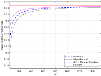
(a)

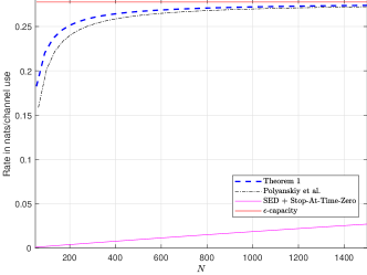
(b)

Figure 1: Achievable rates over (a) the BSC with flip probability 0.11 and (b) the cascade of a BSC with flip probability 0.11 and the binary erasure channel with erasure probability 0.2 are shown with error probability $\epsilon=10^{-3}$.

Our second result is a second-order achievability bound for VLF codes, where the error probability $\epsilon\in(0,1)$ is fixed as the average decoding time $N$ approaches infinity.

Theorem 2

Assume that $C>0$ and $C_{1}<\infty$. Then,

$$\log M^{*}(N,\epsilon)\geq\frac{NC}{1-\epsilon}-\frac{C}{C_{1}}\log N-\log\log N+O(1).$$ (30)

Since $C\leq C_{1}$, Theorem 2 improves the second-order term in [9, eq. (18)] given in the lower bound in (2) from $-\log N$ to $-\frac{C}{C_{1}}\log N$. The achievability bound in [9, eq. (18)] employs stop-feedback while our Yamamoto–Itoh scheme employs stop-feedback and also sends a $\lceil\log_{2}M\rceil$-bits of feedback at the end of the first communication phase. The improvement in the second-order term results from the fact that the error probability of our scheme is dominated by the error probability terms due to the confirmation phase and the second communication phase, whose average length scales as the logarithm of the average length of the first communication phase. For general DMCs, the non-asymptotic bound in [18, Remark 4] for Naghshvar et al.’s MaxEJS encoder achieves a second-order term $-\left(\frac{C}{C_{1}}+1\right)\log N$ when combined with the stop-at-time-zero strategy. To the best of our knowledge, Theorem 2 yields the best asymptotic achievability bound for VLF codes with non-vanishing error probabilities over general DMCs. For BSCs and BACs, Yang et al.’s bounds from [19, Th. 4 and 7] recover (30) with $-\log\log N+O(1)$ improved to $O(1)$ when combined with the stop-at-time-zero strategy. It remains open to close the gap between the achievability bound in Theorem 2 and the converse bound on the right-hand side of (2). The proof of Theorem 2 follows from carefully choosing the parameters $\gamma_{1},\gamma_{2},a_{\mathrm{A}}$, $a_{\mathrm{R}}$, and $\epsilon_{0}$ in Theorem 1, and appears in Section VI-B.

The third result is a second-order achievability bound for universal VLF codes, where the DMC $P_{Y|X}$ is unknown but a capacity-achievability input distribution $P_{X}$ is known. We assume that the error probability $\epsilon\in(0,1)$ is non-vanishing as the average decoding time $N$ approaches infinity.

Theorem 3

Assume that a capacity-achieving distribution of $P_{Y|X}$ is known. Assume that $C>0$ and $C_{1}<\infty$. Assume that $\lim\limits_{N\to\infty}\frac{\ell}{\log N}=\infty$. Then,

$$\log M^{*}_{\mathrm{U}}(N,\epsilon,\ell)\geq\frac{NC}{1-\epsilon}-\frac{C}{C_{1}}\log N$$

$$-\min\left\{\frac{|\mathcal{X}||\mathcal{Y}|}{2},\left(|\mathcal{X}|-\frac{3}{2}\right)\left(|\mathcal{Y}|-\frac{3}{2}\right)+\frac{3}{4}\right\}\log N$$

$$+o(\log N).$$ (31)

In the case where $P_{Y|X}$ is known to be a BSC with an unknown flip probability $p\in(0,1)\setminus\{\frac{1}{2}\}$, (31) is improved to

$$\log M_{\mathrm{U}}^{*}(N,\epsilon,\ell) \geq\frac{NC}{1-\epsilon}-\left(\frac{C}{C_{1}}+\frac{1}{2}\right)\log N+o(\log N).$$ (32)

The coding scheme to achieve the right-hand side of (31) universalizes the coding scheme described in (23)-(27) by (1) replacing the information density $\imath(\mathbf{c}^{n}(m);Y^{n})$ in (23) by the empirical mutual information $nI(\hat{P}_{\mathbf{c}^{n}(m)};\hat{P}_{Y^{n}|\mathbf{c}^{n}(m)})$; (2) replacing the DMC $P_{Y|X}$ in (14)–(27) by the empirical channel transition kernel observed in the training sequence, i.e., $\hat{P}_{\bar{Y}^{\ell}|x^{\ell}}$; and (3) choosing the parameters $\gamma_{1},\gamma_{2},a_{\mathrm{A}},a_{\mathrm{R}}$, and $\epsilon_{0}$ as a function of $M,|\mathcal{X}|,|\mathcal{Y}|$, and $\epsilon$ only. The joint empirical distribution $\hat{P}_{\mathbf{c}^{n}(m)}\times\hat{P}_{Y^{n}|\mathbf{c}^{n}(m)}$ coincides with the maximum likelihood estimator within the family of distributions with alphabets $\mathcal{X}\times\mathcal{Y}$. In the scenario where no training sequence is available, i.e., $\ell=0$, using our proof techniques, we can show that the right-hand sides of (31) and (32) are achievable with the factor $\frac{C}{C_{1}}$ replaced by 1; this result follows by employing a single communication phase.

In [26], in the HT phase, instead of the empirical channel obtained from a training sequence, a BSC-specific metric that is independent of the flip probability, i.e., the difference between the number of 1’s and the number of 0’s, is used. Although the resulting reliability function associated with their universal sequential HT phase is optimal, both the average stopping time and the error probability exponent depend on the unknown flip probability of the BSC. In result, both the rate and the error probability of the code in [26] depend on the unknown capacity value. Since our goal is to control the error probability of the universal code prior to the communication, we instead appeal to the training sequence to use in the log-likelihood ratio during the HT phase.

The proof of Theorem 3 differs from the proof of Theorem 2 in two main ways. First, we bound $\mathbb{P}\left[\tau_{2}^{(i)}\leq n_{2}\right]\leq\sum_{n=1}^{n_{2}}\mathbb{P}\left[nI(\hat{P}_{\bar{X}^{n}},\hat{P}_{Y^{n}|\bar{X}^{n}})>\gamma_{i}\right]$ using the refined method of types bound from [30, Th. 3] and a refined bound on $\mathbb{E}\left[\exp\{nI(\hat{P}_{\bar{X}^{n}},\hat{P}_{Y^{n}|\bar{X}^{n}})\}\right]$. Here, $n_{2}$ is a suitably chosen constant and $(\bar{X},Y)\sim P_{X}P_{Y}$. The third term on the right-hand side of (31) results from the additional multiplicative factor of $n_{2}^{d}$ in the bound on $\mathbb{P}\left[\tau_{m}^{(i)}\leq n_{2}\right]$ compared to (28), where $-d$ is the coefficient of the third term on the right-hand side of (31). Second, to bound the expected stopping time, we use [29, Th. 4.5] from the nonlinear renewal theory, which bounds the expected value of the stopping time $\tau=\inf\{n\geq 1\colon ng\left(\frac{1}{n}S_{n}\right)>\gamma\}$, where $S_{n}$ is a sum of $n$ i.i.d. vectors, and $g$ is a sufficiently smooth function. After we apply this result with $g$ being the mutual information function and $S_{n}$ being the empirical joint distribution of $\mathbf{c}^{n}(1)$ and $Y^{n}$, we get

$$\mathbb{E}\left[\tau^{(i)}\right]\leq\mathbb{E}\left[\tau_{1}^{(i)}\right]\leq\frac{\gamma_{i}}{C}+O(1).$$ (33)

This implies that the expected stopping time associated with the empirical mutual information admits the same asymptotic bound associated with the information density (29) up to an $O(1)$ gap. The analysis in [26] yields the bound $\mathbb{E}\left[\tau^{(i)}\right]\leq\frac{\gamma_{i}}{C}(1+o(1))$ as $\gamma_{i}\to\infty$, which is not sharp enough to prove the $\log N$ scaling of the second-order term in (31). To prove (32), we replace the decoding metric by $n(\log 2-H(\hat{P}_{Z^{n}(m)}))$, where $Z_{i}(m)=|Y_{i}-\mathbf{c}_{i}(m)|$, i.e., the Hamming distance between $Y_{i}$ and $\mathbf{c}_{i}(m)$, for $i\in[n]$. The proof of Theorem 3 is given in Section VII.

For an arbitrary DMC $P_{Y|X}$ and arbitrary random coding input distribution $P_{X}$, our universal code achieves the right-hand side of (31) with the capacity $C$ replaced by the mutual information $I(P_{X},P_{Y|X})$.

V Gaussian Channel

The output of a memoryless Gaussian channel of blocklength $n$ in response to the input $X^{n}\in\mathbb{R}^{n}$ is

$$Y^{n}=X^{n}+Z^{n},$$ (34)

where $Z_{1},\ldots,Z_{n}$ are drawn i.i.d. from $\mathcal{N}(0,\sigma_{0}^{2})$, independent of $X^{n}$, and $\sigma_{0}^{2}>0$ is the noise variance. The capacity function of the Gaussian channel is given by

$$C(S) \triangleq\frac{1}{2}\log(1+S).$$ (35)

The analog of the quantity $C_{1}$ in (6) for the Gaussian channel is defined as

$$C_{1}(S) \triangleq D(\mathcal{N}(\sqrt{S},1)\|\mathcal{N}(-\sqrt{S},1))=2S.$$ (36)

Definition 3

An $(N,M,\epsilon,P)$-VLF code and an $(N,M,\epsilon,\ell,P)$-UVLF code are defined similarly to Definitions 1 and 2 with the addition of average power constraints

$$\mathbb{E}\left[\sum_{t=1}^{\tau}\mathsf{f}_{t}(U,W,Y^{t-1},\sigma_{0}^{2})^{2}\right]\leq\mathbb{E}\left[\tau\right]P,$$ (37)

$$\mathbb{E}\left[\sum_{t=1}^{\tau}\mathsf{f}_{t}(U,W,Y^{t-1},\bar{Y}^{\ell})^{2}\right]\leq\mathbb{E}\left[\tau\right]P,$$ (38)

respectively, where $\tau$ is the random decoding time, $P$ is the average power, and $\bar{Y}^{\ell}$ is the output of the training sequence $x^{\ell}=(0,\dots,0)$. We define the maximum achievable codebook sizes $M^{*}(N,\epsilon,P)$ and $M^{*}_{\mathrm{U}}(N,\epsilon,\ell,P)$ similarly to (12)–(13).

The average power constraint in (37) is introduced in [16] for variable-length stop-feedback codes for the Gaussian multiple-access channel.

The following achievability bounds extend Theorems 2 and 3 to the Gaussian channel with an average power constraint.

Theorem 4

Let $\sigma_{0}^{2}>0$ be the noise variance of the Gaussian channel and let $P$ be the average power constraint. Define the signal-to-noise ratio

$$S\triangleq\frac{P}{\sigma_{0}^{2}}.$$ (39)

For the Gaussian channel with the noise variance $\sigma_{0}^{2}$,

$$\log M^{*}(N,\epsilon,P) \geq\frac{NC(S)}{1-\epsilon}-\frac{C(S)}{C_{1}(S)}\log N$$

$$\quad-\log\log N+O(1).$$ (40)

Proof:

Theorem 4 is proved using our Yamamoto–Itoh scheme described in (21)–(28). During the communication phases, i.e., the C1 and C2 phases, the input symbols are drawn i.i.d. from the Gaussian distribution $\mathcal{N}(0,P)$, which satisfies the average power constraint in (37). During the HT phase, the transmitter sends either $(\sqrt{P},\sqrt{P},\dots)$ or $(-\sqrt{P},-\sqrt{P},\dots)$ to accept or reject the receiver’s initial estimate, respectively. Since the techniques used in the proof of Theorem 1 applies to continuous random variables, Theorem 1 applies to the Gaussian channel with $P_{X}=\mathcal{N}(0,P)$, $P_{Y|X=x}=\mathcal{N}(x,\sigma_{0}^{2})$, and $C=C(S)$. Theorem 4 follows by following the same steps as in the proof of Theorem 2. ∎

Since $C_{1}(S)<C(S)$ for every $S>0$, Theorem 4 improves the second-order term in the achievability bound in [33, Th. 1] from $-\log N$ to $-\frac{C(S)}{C_{1}(S)}\log N$. As an analog to the DMC scenario in (2), in [33, Th. 1], Truong and Tan show the converse bound

$$\log M^{*}(N,\epsilon,P) \leq\frac{NC(S)}{1-\epsilon}+\frac{h_{\mathrm{b}}(\epsilon)}{1-\epsilon}.$$ (41)

Theorem 5

Suppose that $\lim\limits_{N\to\infty}\frac{\ell}{\log N}=\infty$. Under the setting of Theorem 4,

$$\log M^{*}_{\mathrm{U}}(N,\epsilon,\ell,P) \geq\frac{NC(S)}{1-\epsilon}-\left(\frac{C(S)}{C_{1}(S)}+\frac{1}{2}\right)\log N$$

$$\quad+o(\log N).$$ (42)

Theorem 5 refines the achievability result in [27, Th. 4] to the second-order term for the Gaussian channel. To prove Theorem 5, we replace the empirical mutual information $nI(\hat{P}_{X^{n}},\hat{P}_{Y^{n}|X^{n}})$ used in the DMC case with

$$\imath_{\mathrm{U}}(X^{n};Y^{n})\triangleq-\frac{n}{2}\log(1-\hat{\rho}_{X^{n}Y^{n}}^{2}),$$ (43)

where $\hat{\rho}_{X^{n}Y^{n}}$ is the empirical correlation coefficient for zero-mean pairs defined as

$$\hat{\rho}_{X^{n}Y^{n}}\triangleq\frac{\frac{1}{n}\sum_{i=1}^{n}X_{i}Y_{i}}{\sqrt{\frac{1}{n}\sum_{i=1}^{n}X_{i}^{2}}\sqrt{\frac{1}{n}\sum_{i=1}^{n}Y_{i}^{2}}}.$$ (44)

Recall that for zero-mean, jointly Gaussian $(X,Y)$, the mutual information $I(P_{X},P_{Y|X})$ is given by

$$I(P_{X},P_{Y|X})=-\frac{1}{2}\log(1-\rho_{XY}^{2}),$$ (45)

where $\rho_{XY}$ is the correlation coefficient between $X$ and $Y$. The universal quantity $\imath_{\mathrm{U}}(X^{n};Y^{n})$ can be viewed as the empirical mutual information for the Gaussian channel in the sense that

$$\imath_{\mathrm{U}}(X^{n};Y^{n})=nI(\hat{P}_{X^{n}}^{\mathrm{ML}},\hat{P}_{Y^{n}|X^{n}}^{\mathrm{ML}}),$$ (46)

where $(\hat{P}_{X^{n}}^{\mathrm{ML}},\hat{P}_{Y^{n}|X^{n}}^{\mathrm{ML}})$ is the maximum likelihood estimator within the family of jointly-Gaussian distributions. The proof of Theorem 5 appears in Section VIII.

VI Proofs of Theorems 1 and 2

VI-A Proof of Theorem 1

VI-A1 Error probability analysis

Define the error events

$$\mathcal{E}^{(i)} \triangleq\{\hat{W}^{(i)}\neq 1\},\quad i=1,2$$ (47)

$$\mathcal{E}_{\mathrm{A}\to\mathrm{R}} \triangleq\{\mathrm{H}_{\mathrm{R}}\text{ is declared given }\mathrm{H}_{\mathrm{A}}\}$$ (48)

$$\mathcal{E}_{\mathrm{R}\to\mathrm{A}} \triangleq\{\mathrm{H}_{\mathrm{A}}\text{ is declared given }\mathrm{H}_{\mathrm{R}}\}$$ (49)

$$\mathcal{E}_{\mathrm{C2}} \triangleq\{\text{C2 phase is entered}\}.$$ (50)

Then the error probability of the above scheme is bounded as

$$\mathbb{P}\left[\hat{W}\neq 1\right] \leq\mathbb{P}\left[(\mathcal{E}^{(1)}\bigcap\mathcal{E}_{\mathrm{R}\to\mathrm{A}})\bigcup\mathcal{E}^{(2)}\right]$$ (51)

$$\leq\mathbb{P}\left[\mathcal{E}^{(1)}\right]\mathbb{P}\left[\mathcal{E}_{\mathrm{R}\to\mathrm{A}}\right]+\mathbb{P}\left[\mathcal{E}^{(2)}\right],$$ (52)

where (52) follows from the union bound and the independence of the events $\mathcal{E}^{(1)}$ and $\mathcal{E}_{\mathrm{R}\to\mathrm{A}}$. From [29, Th. 3.1], the type-I and type-II error probabilities of the sequential hypothesis test is bounded as

$$\mathbb{P}\left[\mathcal{E}_{\mathrm{A}\to\mathrm{R}}\right] \leq\exp\{-a_{\mathrm{R}}\}$$ (53)

$$\mathbb{P}\left[\mathcal{E}_{\mathrm{R}\to\mathrm{A}}\right] \leq\exp\{-a_{\mathrm{A}}\}.$$ (54)

The probabilities $\mathbb{P}\left[\mathcal{E}^{(i)}\right]$, $i=1,2$, are bounded following [9, Proof of Th. 2] as

$$\mathbb{P}\left[\mathcal{E}^{(i)}\right] \leq\mathbb{P}\left[\tau^{(i)}_{1}=\infty\right]+\mathbb{P}\left[\bigcup_{m=2}^{M}\{\tau^{(i)}_{m}<\infty\}\right]$$ (55)

$$\leq(M-1)\exp\{-\gamma_{i}\},\quad i=1,2.$$ (56)

Combining (52), (54), and (56), we get

$$\mathbb{P}\left[\hat{W}\neq 1\right] \leq(M-1)\left(\exp\{-(\gamma_{1}+a_{\mathrm{A}})\}+\exp\{-\gamma_{2}\}\right).$$ (57)

VI-A2 Average decoding time analysis

We use the following result from the renewal theory literatur, which bounds the expected value of the stopping time associated with a random walk.

Lemma 1 ([32, Th. 1], [34, Ch. 3, Th. 9.2–9.3, Th. 10.7])

Let $X,X_{1},X_{2},\dots$ be i.i.d. random variables with $\mathbb{E}\left[X\right]=\mu>0$ and $\mathbb{E}\left[(X^{+})^{2}\right]<\infty$. Let $S_{n}=\sum_{i=1}^{n}X_{i}$ and $\tau=\inf\{n\geq 1\colon S_{n}>a\}$. Then, for any $a>0$,

$$\mathbb{E}\left[\tau\right]\leq\frac{1}{\mu}\left(a+b(X)\right).$$ (58)

Let

$$\tau_{+} =\inf\{n\geq 1\colon S_{n}>0\}$$ (59)

$$\rho =\frac{\mathbb{E}\left[S^{2}_{\tau_{+}}\right]}{2\mathbb{E}\left[S_{\tau_{+}}\right]}.$$ (60)

As $a\to\infty$, if $X$ is non-arithmetic and the above conditions are satisfied, then

$$\mathbb{E}\left[\tau\right]=\frac{1}{\mu}\left(a+\rho\right)+o(1),$$ (61)

and if $X$ is arithmetic with a span $h$ and $a=jh$, $j\to\infty$, then

$$\mathbb{E}\left[\tau\right]=\frac{1}{\mu}\left(a+\rho+\frac{h}{2}\right)+o(1).$$ (62)

It holds that

$$\frac{\mathbb{E}\left[S^{2}_{\tau_{+}}\right]}{2\mathbb{E}\left[S_{\tau_{+}}\right]}=\frac{\mathbb{E}\left[X^{2}\right]}{2\mu}-\sum_{k=1}^{\infty}\frac{1}{k}\mathbb{E}\left[S_{k}^{-}\right].$$ (63)

We bound the probability that the C2 phase is used as

$$\mathbb{P}\left[\mathcal{E}_{\mathrm{C2}}\right] =\mathbb{P}\left[(\mathcal{E}^{(1)}\cap\mathcal{E}_{\mathrm{R}\to\mathrm{A}}^{\mathrm{c}})\cup((\mathcal{E}^{(1)})^{\mathrm{c}}\cap\mathcal{E}_{\mathrm{A}\to\mathrm{R}})\right]$$ (64)

$$\leq\mathbb{P}\left[\mathcal{E}^{(1)}\right]+\mathbb{P}\left[\mathcal{E}_{\mathrm{A}\to\mathrm{R}}\right]$$ (65)

$$\leq(M-1)\exp\{-\gamma_{1}\}+\exp\{-a_{\mathrm{R}}\}.$$ (66)

Recall the stopping times defined in (22)–(23). Obviously, it holds that $\tau^{(i)}_{1}\leq\tau^{(i)}$ for $i=1,2$. By our code design, $\tau=\tau^{(1)}+\tau^{\mathrm{HT}}$ if the event $\mathcal{E}_{\mathrm{C2}}$ does not occur and $\tau=\tau^{(2)}+\tau^{\mathrm{HT}}$ if $\mathcal{E}_{\mathrm{C2}}$ occurs. Then, we bound the average stopping time as

$$\mathbb{E}\left[\tau\right]\leq\mathbb{E}\left[\tau^{\mathrm{HT}}\right]+\mathbb{E}\left[\tau^{(1)}_{1}\right]+\mathbb{P}\left[\mathcal{E}_{\mathrm{C2}}\right]\mathbb{E}\left[\tau^{(2)}_{1}-\tau^{(1)}_{1}\right].$$ (67)

Applying Lemma 1, we bound each of the expectations in (67) as

$$\mathbb{E}\left[\tau_{\mathrm{HT}}|H_{\mathrm{A}}\right] \leq\frac{a_{\mathrm{A}}+b_{\mathrm{A}}}{D(P_{Y|X=x_{\mathrm{A}}}\|P_{Y|X=x_{\mathrm{R}}})}$$ (68)

$$\mathbb{E}\left[\tau_{\mathrm{HT}}|H_{\mathrm{R}}\right] \leq\frac{a_{\mathrm{R}}+b_{\mathrm{R}}}{D(P_{Y|X=x_{\mathrm{R}}}\|P_{Y|X=x_{\mathrm{A}}})}$$ (69)

$$\mathbb{E}\left[\tau_{\mathrm{HT}}\right] \leq\mathbb{E}\left[\tau_{\mathrm{HT}}|H_{\mathrm{A}}\right]+\mathbb{P}\left[H_{\mathrm{R}}\right]\mathbb{E}\left[\tau_{\mathrm{HT}}|H_{\mathrm{R}}\right]$$ (70)

$$\leq\mathbb{E}\left[\tau_{\mathrm{HT}}|H_{\mathrm{A}}\right]$$

$$\quad+(M-1)\exp\{-\gamma_{1}\}\mathbb{E}\left[\tau_{\mathrm{HT}}|H_{\mathrm{R}}\right]$$ (71)

$$\mathbb{E}\left[\tau^{(1)}_{1}\right] \leq\frac{\gamma_{1}+b}{C}$$ (72)

$$\mathbb{E}\left[\tau^{(2)}_{1}-\tau^{(1)}_{1}\right] \leq\frac{\gamma_{2}-\gamma_{1}+b}{C},$$ (73)

where $b=b(\imath(X;Y))$, $b_{\mathrm{A}}=b\left(\log\frac{P_{Y|X=x_{\mathrm{A}}}(Y_{\mathrm{A}})}{P_{Y|X=x_{\mathrm{R}}}(Y_{\mathrm{A}})}\right)$, and $b_{\mathrm{R}}=b\left(\log\frac{P_{Y|X=x_{\mathrm{R}}}(Y_{\mathrm{R}})}{P_{Y|X=x_{\mathrm{A}}}(Y_{\mathrm{R}})}\right)$, and and $Y_{\mathrm{D}}$ is distributed according to $P_{Y|X=x_{\mathrm{D}}}$ for $\mathrm{D}\in\{\mathrm{A},\mathrm{R}\}$.

Finally, combining (66), (67), and (71)–(73) gives

$$\mathbb{E}\left[\tau\right] \leq\frac{\gamma_{1}+b}{C}$$

$$+((M-1)\exp\{-\gamma_{1}\}+\exp\{-a_{\mathrm{R}}\})\frac{\gamma_{2}-\gamma_{1}+b}{C}$$

$$+\frac{a_{\mathrm{A}}+b_{\mathrm{A}}}{D(P_{Y|X=x_{\mathrm{A}}}\|P_{Y|X=x_{\mathrm{R}}})}$$

$$+(M-1)\exp\{-\gamma_{1}\}\frac{a_{\mathrm{R}}+b_{\mathrm{R}}}{D(P_{Y|X=x_{\mathrm{R}}}\|P_{Y|X=x_{\mathrm{A}}})}.$$ (74)

From the above analysis, there exists an $(N^{\prime},M,\epsilon^{\prime})$-VLF code with $\epsilon^{\prime}$ and $N^{\prime}$ are given as the right hand sides of (57) and (74), respectively. We use the stop-at-time-zero strategy described in [9], where with probability $1-\epsilon_{0}$, the code above is used, and with probability $\epsilon_{0}$, we use a simple code that stops at time zero and decodes to an arbitrary message. Let $N$ and $\epsilon$ be the average decoding time and the average error probability of the described code obtained by this time-sharing strategy. We have

$$N \leq(1-\epsilon_{0})N^{\prime}$$ (75)

$$\epsilon \leq\epsilon_{0}+(1-\epsilon_{0})\epsilon^{\prime},$$ (76)

which completes the proof.

VI-B Proof of Theorem 2

We prove Theorem 2 by carefully choosing the free parameters $\gamma_{1},\gamma_{2},a_{\mathrm{A}},a_{\mathrm{R}}$, and $\epsilon_{0}$ in Theorem 1. Let

$$N_{1}=\frac{\gamma_{1}+b}{C},$$ (77)

which is an upper bound on the expected length of phase C1. We express all other parameters in terms of $N_{1}$. We set

$$\gamma_{1} =\log M+\log\log N_{1}$$ (78)

$$\gamma_{2} =\log M+\log N_{1}$$ (79)

$$a_{\mathrm{A}} =a_{\mathrm{R}}=\log N_{1}.$$ (80)

Then, by (18), we have as $N_{1}\to\infty$

$$N^{\prime} =N_{1}+\frac{\log N_{1}}{C_{1}}+O(1)$$ (81)

$$\epsilon^{\prime} \leq\frac{1}{N_{1}}\left(1+\frac{1}{\log N_{1}}\right).$$ (82)

We set

$$\epsilon_{0}=\frac{\epsilon-\frac{1}{N_{1}}\left(1+\frac{1}{\log N_{1}}\right)}{1-\frac{1}{N_{1}}\left(1+\frac{1}{\log N_{1}}\right)}=\epsilon-\Omega\left(\frac{1}{N_{1}}\left(1+\frac{1}{\log N_{1}}\right)\right).$$ (83)

From (77) and (78), we get

$$\log M=N_{1}C-\log\log N_{1}+O(1).$$ (84)

From (81) and (84), we get

$$\log M=N^{\prime}C-\frac{C}{C_{1}}\log N^{\prime}-\log\log N^{\prime}+O(1).$$ (85)

Finally, from (16) and (83), the error probability of the code is bounded by $\epsilon$, and the average decoding time of the code is bounded by $(1-\epsilon_{0})N^{\prime}$. Therefore, by (81) and (85), there exists an $(N,M,\epsilon)$-VLF code with

$$\log M=\frac{NC}{1-\epsilon}-\frac{C}{C_{1}}\log N-\log\log N+O(1).$$ (86)

VII Proof of Theorem 3

VII-A Supporting Lemmas

We first present two supporting lemmas that play key roles to prove Theorem 3. The first result, below, bounds the tail probability of the empirical mutual information for independent $\bar{X}^{n}$ and $Y^{n}$.

Lemma 2

Let $(\bar{X}^{n},Y^{n})\sim P_{X}^{n}P_{Y}^{n}$ for some $P_{X}\in\mathcal{P}(\mathcal{X})$ and $P_{Y}\in\mathcal{P}(\mathcal{Y})$, and let $\gamma$ be a positive constant. Assume that $P_{X}(x)>0$ and $P_{Y}(y)>0$ for all $(x,y)\in(\mathcal{X}\times\mathcal{Y})$. Then, there exists $n_{0}\in\mathbb{N}$ such that for all $n\geq n_{0}$

$$\mathbb{P}\left[nI(\hat{P}_{\bar{X}^{n}Y^{n}})\geq\gamma\right]\leq K_{1}(n+1)^{k}\exp\{-\gamma\}$$ (87)

$$k=\min\left\{{\frac{|\mathcal{X}||\mathcal{Y}|-2}{2}},{\left(|\mathcal{X}|-\frac{3}{2}\right)\left(|\mathcal{Y}|-\frac{3}{2}\right)-\frac{1}{4}}\right\},$$ (88)

where $K_{1}$ is a positive constant depending only on $|\mathcal{X}|$ and $|\mathcal{Y}|$.

Proof:

See Appendix A. ∎

The second result, which is from the nonlinear renewal theory literature, bounds the expected stopping time associated with a function of an i.i.d. sum. This result is the nonlinear version of Lemma 1 and is used to bound the expected stopping times associated with the empirical mutual information.

Lemma 3

[29, Th. 4.5] Let $g\colon\mathbb{R}^{k}\to\mathbb{R}$ be a twice differentiable continuous function. Let $Y,Y_{1},Y_{2},\dots\in\mathbb{R}^{k}$ be i.i.d. random vectors. Let $\mu=g(\mathbb{E}\left[Y\right])>0$. Let $\gamma>0$. Define

$$Z_{n} =ng\left(\frac{1}{n}\sum_{i=1}^{n}Y_{i}\right)$$ (89)

$$\tau =\inf\{n\geq 1\colon Z_{n}>a\}.$$ (90)

Then, if $\mu+\nabla g(\mathbb{E}\left[Y\right])^{\top}(Y-\mathbb{E}\left[Y\right])$ is non-arithmetic, as $a\to\infty$,

$$\mathbb{E}\left[\tau\right]=\frac{1}{\mu}\left(a+\rho-\frac{1}{2}\mathrm{tr}(\mathrm{Cov}(Y)\nabla^{2}g(\mathbb{E}\left[Y\right]))\right)+o(1),$$ (91)

where $\rho$ is defined in (60) with $S_{n}=\sum_{i=1}^{n}X_{i}$ replaced with $n\mu+\sum_{i=1}^{n}\nabla g(\mathbb{E}\left[Y\right])^{\top}(Y_{i}-\mathbb{E}\left[Y\right])$. If $\mu+\nabla g(\mathbb{E}\left[Y\right])^{\top}(Y-\mathbb{E}\left[Y\right])$ is arithmetic with a span $h>0$, then as $a\to\infty$,

$$\mathbb{E}\left[\tau\right]=\frac{1}{\mu}\left(a+\rho+\frac{h}{2}-\frac{1}{2}\mathrm{tr}(\mathrm{Cov}(Y)\nabla^{2}g(\mathbb{E}\left[Y\right]))\right)+o(1).$$ (92)

Lemma 3 is a special case of the nonlinear form $Z_{n}=\sum_{i=1}^{n}X_{i}+\xi_{n}$, where $X_{1},X_{2},\dots$ are i.i.d. random variables, $\xi_{n}$’s are slowly changing random variables, which is specified in [29, eq. (4.10)–(4.16)], and $(X_{1},\xi_{1}),\dots,(X_{n},\xi_{n})$ are independent of $X_{k},k>n$. From the Taylor series expansion of $Z_{n}$ around $ng(\mathbb{E}\left[Y\right])$, we get

$$Z_{n}=n\mu+\sum_{i=1}^{n}\nabla g(\mathbb{E}\left[Y\right])^{\top}(Y_{i}-\mathbb{E}\left[Y\right])$$

$$+\frac{1}{2}W_{n}^{\top}\nabla^{2}g(\mathbb{E}\left[Y\right])W_{n}+o(1)$$ (93)

$$W_{n}=\frac{1}{\sqrt{n}}\sum_{i=1}^{n}(Y_{i}-\mathbb{E}\left[Y\right]).$$ (94)

Therefore, in Lemma 3, $\mu+\nabla g(\mathbb{E}\left[Y\right])^{\top}(Y_{i}-\mathbb{E}\left[Y\right])$ plays the role of $X_{i}$ and $\frac{1}{2}W_{n}^{\top}\nabla^{2}g(\mathbb{E}\left[Y\right])W_{n}+o(1)+o(1)$ plays the role of $\xi_{n}$. In [29, Example 4.1], it is shown that $W_{n}$ satisfies the slowly-changing conditions. By the central limit theorem, $W_{n}$ approaches the Gaussian vector $\mathcal{N}(0,\mathrm{Cov}(Y))$ in distribution, and the third-term in (93) approaches the sum of $k$ independent $\chi^{2}(1)$ random variables, weighted with $\frac{1}{2}$ times the eigenvalues of the matrix $\mathrm{Cov}(Y)\nabla^{2}g(\mathbb{E}\left[Y\right])$.

VII-B Universal Coding Scheme

We generate $M$ i.i.d. codewords $\mathbf{c}(1),\dots,\mathbf{c}(M)$ from $P_{X}^{\infty}$. Our coding scheme is similar to that in Section VI-A except that we replace the information-density decoding metric with the empirical mutual information. Specifically, the stopping times $\tau_{m}^{(i)}$ in (22) are replaced with

$$\tau_{m}^{(i)} =\inf\{n\geq 1\colon nI(\hat{P}_{\mathbf{c}^{n}(m)},\hat{P}_{Y^{n}|\mathbf{c}^{n}(m)})>\gamma_{i}\}.$$ (95)

In the HT phase, since $P_{Y|X}$ is unknown, the log-likelihood ratio test is modified as follows. Define

$$\tilde{P}_{Y|X=x}\triangleq\hat{P}_{Y^{\ell_{x}}|X^{\ell_{x}}=x^{\ell_{x}}},$$ (96)

where $\ell_{x}$ is the number of $x\in\mathcal{X}$ in the training sequence $x^{\ell}$. A lower bound on $\tau^{(1)}$ is

$$n_{1}=\left\lfloor\frac{\log M}{\min\{|\mathcal{X}|,|\mathcal{Y}|\}}\right\rfloor.$$ (97)

Define the event

$$\mathcal{G}\triangleq\left\{\max_{(x,y)}|\tilde{P}_{Y|X=x}(y)-P_{Y|X=x}(y)|=o(1)\right\}.$$ (98)

By the assumption that $\frac{\ell}{\log N}\to\infty$, using Hoeffding’s bound, we have

$$\mathbb{P}\left[\mathcal{G}^{\mathrm{c}}\right]\leq\frac{1}{n_{1}^{2}}.$$ (99)

We re-define $(x_{\mathrm{A}},x_{\mathrm{R}})$ in (14) and the stopping time $\tau_{\mathrm{HT}}$ in (27) by replacing $P_{Y|X}$ by the empirical conditional distribution $\hat{P}_{Y|X}$. Given that $\mathcal{G}$ occurs, the modified $x_{\mathrm{A}}$ and $x_{\mathrm{R}}$ coincide with those in (14).

VII-C Analysis

We here explain the differences from the proof of Theorem 2.

1. Let $n_{2}=c_{2}\frac{\gamma_{2}}{C}$, where $c_{2}>1$ is a constant. We bound the probability $\mathbb{P}\left[\mathcal{E}^{(i)}\right]$ as

   $$\mathbb{P}\left[\mathcal{E}^{(i)}\right]\leq\mathbb{P}\left[\tau^{(i)}_{1}\geq n_{2}\right]+\mathbb{P}\left[\bigcup_{m=2}^{M}\{\tau^{(i)}_{m}<n_{2}\}\right]$$ (100)

   $$\leq\mathbb{P}\left[n_{2}I(\hat{P}_{\mathbf{c}^{n_{2}}(1)Y^{n_{2}}})\leq\gamma_{i}\right]$$

   $$+(M-1)(n_{2}-n_{1})$$

   $$\max\limits_{n\in[n_{1},n_{2}-1]}\mathbb{P}\left[nI(\hat{P}_{\mathbf{c}^{n}(2)},\hat{P}_{Y^{n}|\mathbf{c}^{n}(2)})>\gamma_{i}\right]$$ (101)

   $$\leq n_{2}^{|\mathcal{X}||\mathcal{Y}|}\exp\{-c_{3}\gamma_{i}\}+K_{1}Mn_{2}^{d}\exp\{-\gamma_{i}\},$$ (102)

   where $c_{3}$ and $K_{1}$ are positive constants, and $d=\min\left\{\frac{|\mathcal{X}||\mathcal{Y}|}{2},\left(|\mathcal{X}|-\frac{3}{2}\right)\left(|\mathcal{Y}|-\frac{3}{2}\right)+\frac{3}{4}\right\}$. Here, (101) follows from the definition of $\tau^{(i)}$ and the union bound across time and messages; the first term in (102) follows from the standard method of types (see e.g., [26, Lemma 3]), and the second term in (102) follows from Lemma 2.

2. We bound the expected value of the stopping times $\tau^{(i)}$, $i=1,2$, using Lemma 3 instead of Lemma 1. To do this, we write the empirical mutual information as

   $$nI(\hat{P}_{X^{n}},\hat{P}_{Y^{n}|X^{n}})=nI\left(\sum_{i=1}^{n}V_{i}\right)$$ (103)

   $$=\sum_{i=1}^{n}\imath(X_{i};Y_{i})+\frac{1}{2}W_{n}^{\top}\nabla^{2}I(P_{X},P_{Y|X})W_{n}+o(1)$$ (104)

   $$W_{n}=\frac{1}{\sqrt{n}}\sum_{i=1}^{n}(V_{i}-\mathbb{E}\left[V_{i}\right]),$$ (105)

   where $V_{i}\in\mathbb{R}^{|\mathcal{X}||\mathcal{Y}|}$, $i=1,\dots,n$, are independent and have multinomial distribution with parameters $(n,P_{XY})$. Hence, $\imath(X^{n};Y^{n})$ is a first-order Taylor approximation to the empirical mutual information $nI(\hat{P}_{X^{n}},\hat{P}_{Y^{n}|X^{n}})$. Applying Lemma 3 to $\mathbb{E}\left[\tau_{1}^{(i)}\right]$, similar to (72)–(73), we get

   $$\mathbb{E}\left[\tau_{1}^{(1)}\right] =\frac{\gamma_{1}}{C}+O(1)$$ (106)

   $$\mathbb{E}\left[\tau_{1}^{(2)}-\tau_{1}^{(1)}\right] =\frac{\gamma_{2}-\gamma_{1}}{C}+O(1).$$ (107)

   Notice that the bound in (106) is asymptotically the same as the bound in (72) except the value of the constant $O(1)$ term.

3. Combining (68)–(69) with (98), we get

   $$\mathbb{E}\left[\tau_{\mathrm{HT}}|H_{\mathrm{A}}\right] \leq\frac{a_{\mathrm{A}}\left(1+o(1)\right)}{D(P_{Y|X=x_{\mathrm{A}}}\|P_{Y|X=x_{\mathrm{R}}})}+O(1)$$ (108)

   $$\mathbb{E}\left[\tau_{\mathrm{HT}}|H_{\mathrm{R}}\right] \leq\frac{a_{\mathrm{R}}\left(1+o(1)\right)}{D(P_{Y|X=x_{\mathrm{R}}}\|P_{Y|X=x_{\mathrm{A}}})}+O(1).$$ (109)

   Combining (54) and (98), we get

   $$\mathbb{P}\left[\mathcal{E}_{\mathrm{A}\to\mathrm{R}}\right] \leq\exp\{-a_{\mathrm{R}}\}(1+o(1))$$ (110)

   $$\mathbb{P}\left[\mathcal{E}_{\mathrm{R}\to\mathrm{A}}\right] \leq\exp\{-a_{\mathrm{A}}\}(1+o(1)).$$ (111)

4. Lastly, the error probability of our UVLF code is bounded as

   $$\mathbb{P}\left[\hat{W}\neq 1\right]\leq\mathbb{P}\left[\mathcal{G}^{\mathrm{c}}\right]+\mathbb{P}\left[\mathcal{E}^{(1)}\right]\mathbb{P}\left[\mathcal{E}_{\mathrm{R}\to\mathrm{A}}\right]+\mathbb{P}\left[\mathcal{E}^{(2)}\right].$$ (112)

The rest of the proof follows steps identical to those in Section VI-A except that the code parameters are chosen independently from $P_{Y|X}$. Since $N_{1}\approx\frac{\log M}{C}$ depends on the channel capacity, unlike the VLF code design, the code parameters for the UVLF code cannot depend on $N_{1}$.

Notice that since the optimal choice for $\gamma_{2}$ satisfies $\gamma_{2}=\log M(1+o(1))$, it holds that $n_{2}=\Theta(N_{1})$. Since $C>0$, it also holds that $n_{1}=\Theta(N_{1})$. To balance the additional factor of $n_{2}^{d}$ in (102) and to get an error probability bound independent of $n_{2}$, we let $\delta>0$ be an arbitrary constant, and we set the thresholds $\gamma_{1}$ and $\gamma_{2}$ slightly larger than those in (78)–(79) as

$$\gamma_{1} =\log M+d\log n_{1}+(1+\delta)\log\log n_{1}$$ (113)

$$\gamma_{2} =\log M+(d+1)\log n_{1}+\delta\log\log n_{1}.$$ (114)

Based on (110)–(111), we set

$$a_{\mathrm{A}} =a_{\mathrm{R}}=\log n_{1}.$$ (115)

Combining (102), the confidence bound in (99), and the error probability bound in (112), (111), and (115), for UVLF codes, $\epsilon^{\prime}$ in (82) is bounded as

$$\epsilon^{\prime} \leq\frac{1}{n_{1}}$$ (116)

for $\log M$ large enough. We set the stopping probability at time zero as

$$\epsilon_{0}=\frac{\epsilon-\frac{1}{n_{1}}}{1-\frac{1}{n_{1}}}.$$ (117)

Following steps similar to those in (84)–(86) with the modifications in (113)–(117) and $n_{1}=\Omega(N_{1})$, we complete the proof of (31).

VII-D Universal Coding Scheme for a BSC Family and Its Analysis

The coding scheme is identical to that in Section VII-B except that the stopping time in (95) is replaced with

$$\tau_{m}^{(i)}\triangleq\inf\{n\geq 1\colon n(\log 2-H(\hat{P}_{Z^{n}(m)}))>\gamma_{i}\},$$ (118)

where $Z_{i}(m)=1\{Y_{i}\neq\mathbf{c}_{i}(m)\}$. Define

$$\hat{p}_{n}(m)\triangleq\frac{1}{n}\sum_{i=1}^{n}Z_{i}(m),$$ (119)

Hence, $H(\hat{P}_{Z^{n}(m)})=h_{\mathrm{b}}(\hat{p}_{n}(m))$ is the binary entropy function of the empirical flip probability from the sub-codeword $\mathbf{c}^{n}(m)$ to the output sequence $Y^{n}$.

We bound the probability $\mathbb{P}\left[\tau_{2}^{(i)}<n_{2}\right]$ differently than (101)–(102). The information density under the BSC($p$) equals

$$\imath(\mathbf{c}^{n}(m);Y^{n})=n\left(\log(2(1-p))-\hat{p}_{n}(m)\log\frac{1-p}{p}\right).$$ (120)

Therefore, both $\tau_{1}^{(i)}$ and $\imath(\mathbf{c}^{n}(1);Y^{n})$ depends on $(\mathbf{c}^{n}(1),Y^{n})$ only through the empirical flip probability $\hat{p}_{n}(1)$. This means that $\tau_{1}^{(i)}$ is a stopping time for the martingale $\{\exp\{-\imath(\mathbf{c}^{n}(1);Y^{n})\}\}_{n\geq 1}$. Using this property, we apply the steps in [9, eq. (111)–(117)] and get

$$\mathbb{P}\left[\tau_{2}^{(i)}<n_{2}\right]=\mathbb{E}\left[\exp\{-\imath(\mathbf{c}^{\tau_{1}^{(i)}}(m);Y^{\tau_{1}^{(i)}})\}1\{\tau_{1}^{(i)}<n_{2}\}\right].$$ (121)

Define

$$R^{(i)} \triangleq\tau_{1}^{(i)}(\log 2-H(\hat{P}_{Z^{\tau_{1}^{(i)}}}))-\gamma_{i}$$ (122)

$$\eta_{n} \triangleq n(\log 2-H(\hat{P}_{Z^{n}(1)}))-\imath(\mathbf{c}^{n}(1);Y^{n}).$$ (123)

Here, $R^{(i)}\geq 0$ is the overshoot random variable corresponding to the transmitted codeword. Then, we bound the right-hand side of (121) as

$$\mathbb{P}\left[\tau_{2}^{(i)}<n_{2}\right]$$

$$=\exp\{-\gamma_{i}\}\mathbb{E}\left[\exp\{-R^{(i)}+\eta_{\tau_{1}^{(i)}}\}1\{\tau_{1}^{(i)}<n_{2}\}\right]$$ (124)

$$\leq\exp\{-\gamma_{i}\}\mathbb{E}\left[\exp\{\eta_{\tau_{1}^{(i)}}\}1\{\tau_{1}^{(i)}<n_{2}\}\right]$$ (125)

$$\leq\max_{n<n_{2}}\mathbb{E}\left[\exp\{\eta_{n}\}\right]\exp\{-\gamma_{i}\}$$ (126)

$$\leq K_{2}\sqrt{n_{2}}\exp\{-\gamma_{i}\},$$ (127)

where $K_{2}$ is a positive constant independent of $n_{2}$ and $\gamma_{i}$. The last step in (127) is proved in Appendix B.

Next, we check that the first-order Taylor series expansion to the universal metric $n(\log 2-H(\hat{P}_{Z^{n}}))$ is equal to the information density $\imath(X^{n};Y^{n})$, where $Z_{i}=1\{Y_{i}\neq X_{i}\}$, $i\in[n]$. Therefore, the asymptotic expansions in (106)–(107) remain to hold.

Comparing (102) with (127), we set $d=\frac{1}{2}$ in (113) and (114), then follow the same steps as in (108)–(117) to complete the proof of (32).

VIII Proof of Theorem 5

The following result is a strong large deviations bound for the correlation coefficient of the two jointly-Gaussian random variables.

Lemma 4 ([35, Th. 3.5])

Let $(X^{n},Y^{n})$ be i.i.d. from $\mathcal{N}(0,\mathsf{\Sigma})$ and $\mathsf{\Sigma}_{12}=0$, i.e., $X_{i}$ and $Y_{i}$ are independent. Let $\hat{\rho}_{X^{n}Y^{n}}=\frac{\frac{1}{n}\sum_{i=1}^{n}X_{i}Y_{i}}{\sqrt{\frac{1}{n}\sum_{i=1}^{n}X_{i}^{2}}\sqrt{\frac{1}{n}\sum_{i=1}^{n}Y_{i}^{2}}}$ be the empirical correlation coefficient. Let $a\in(0,1)$. Then, as $n\to\infty$,

$$\mathbb{P}\left[\hat{\rho}_{X^{n}Y^{n}}\geq a\right] =\frac{(1-4\lambda_{a}^{2})^{-\frac{1}{4}}}{\lambda_{a}\sigma_{a}\sqrt{n}}\exp\left\{\frac{n}{2}\log(1-a^{2})\right\}$$

$$\quad\cdot(1+o(1)),$$ (128)

where

$$\sigma_{a} =\frac{1-a^{2}}{\sqrt{1+a^{2}}}$$ (129)

$$\lambda_{a} =\frac{a}{1-a^{2}}.$$ (130)

VIII-A Universal Coding Scheme for the Gaussian Channel

We here explain the differences from the coding scheme in Section VII-B.

We generate $M$ i.i.d. codewords $\mathbf{c}(1),\dots,\mathbf{c}(M)$ from $P_{X}^{\infty}=\mathcal{N}(0,P)^{\infty}$. The stopping times $\tau_{m}^{(i)}$ in (95) are replaced with

$$\tau_{m}^{(i)}=\inf\{n\geq 1\colon\imath_{\mathrm{U}}(\mathbf{c}^{n}(m);Y^{n})>\gamma_{i}\}.$$ (131)

The empirical channel in (96) that is used in the HT phase is replaced with

$$\tilde{P}_{Y|X=x}=\mathcal{N}\left(x,\frac{1}{\ell}\sum_{i=1}^{\ell}\bar{Y}_{i}^{2}\right),$$ (132)

where the training outputs are distributed i.i.d. as $Y_{i}\sim\mathcal{N}(0,\sigma_{0}^{2})$. Let

$$n_{1}=\lfloor\log M\rfloor,$$ (133)

which satisfies $n_{1}=\Theta(N)$ for any $\sigma_{0}^{2}>0$. We re-define the event $\mathcal{G}$ as

$$\mathcal{G}\triangleq\left\{\left\lvert\frac{1}{\ell}\sum_{i=1}^{\ell}\bar{Y}_{i}^{2}\right\rvert=o(1)\right\}.$$ (134)

By the assumption that $\frac{\ell}{\log N}\to\infty$, applying the Chernoff bound, we get

$$\mathbb{P}\left[\mathcal{G}^{\mathrm{c}}\right]\leq\frac{1}{n_{1}^{2}}.$$ (135)

In the HT phase, we set $x_{\mathrm{A}}=\sqrt{P}$ and $x_{\mathrm{R}}=-\sqrt{P}$ and construct the SPRT in (27) with $P_{Y|X}$ replaced with $\hat{P}_{Y|X}$.

In the following, we explain the differences from the four items in Section VII-C.

1. Let $n_{2}=c_{2}\frac{\gamma_{2}}{C(S)}$, where $c_{2}>1$ is a constant. We bound the probability $\mathbb{P}\left[\mathcal{E}^{(i)}\right]$ as

   $$\mathbb{P}\left[\mathcal{E}^{(i)}\right]\leq\mathbb{P}\left[\tau^{(i)}_{1}\geq n_{2}\right]+\mathbb{P}\left[\bigcup_{m=2}^{M}\{\tau^{(i)}_{m}<n_{2}\}\right]$$ (136)

   $$\leq\mathbb{P}\left[\imath_{\mathrm{U}}(\hat{P}_{\mathbf{c}^{n_{2}}(1)Y^{n_{2}}})\leq\gamma_{i}\right]$$

   $$+(M-1)\sum_{n=1}^{n_{2}}\mathbb{P}\left[\imath_{\mathrm{U}}(\hat{P}_{\mathbf{c}^{n}(2)},\hat{P}_{Y^{n}|\mathbf{c}^{n}(2)})>\gamma_{i}\right]$$ (137)

   $$\leq\exp\{-c_{3}\gamma_{i}\}+K_{1}n_{2}^{1/2}\exp\{-\gamma_{i}\},$$ (138)

   where $c_{3}$ and $K_{1}$ are positive constants independent of $n_{2}$ and $\gamma_{i}$. Here, the first term in (138) follows from the Chernoff bound, and the second term in (138) follows by writing

   $$\mathbb{P}\left[\imath_{\mathrm{U}}(\hat{P}_{\mathbf{c}^{n}(2)},\hat{P}_{Y^{n}|\mathbf{c}^{n}(2)})>\gamma_{i}\right]$$

   $$=\mathbb{P}\left[\hat{\rho}_{\mathbf{c}^{n}(2)Y^{n}}>a\right]$$ (139)

   $$\leq\frac{K_{2}}{\sqrt{n}}\exp\left\{\frac{n}{2}\log(1-a^{2})\right\}(1+o(1)),$$ (140)

   where $a\in(0,1)$ satisfies $\gamma_{i}=-\frac{n}{2}\log(1-a^{2})$, and $K_{2}$ is a positive constant that depends only on $a$. The bound in (140) follows from Lemma 4.

2. Let

   $$\imath^{*}(b_{xy},b_{x},b_{y})\triangleq-\frac{1}{2}\log\left(1-\frac{b_{xy}^{2}}{b_{x}b_{y}}\right).$$ (141)

   Then, we have

   $$\imath_{\mathrm{U}}(X^{n};Y^{n})=n\,\imath^{*}\left(\frac{1}{n}\sum_{i=1}^{n}X_{i}Y_{i},\frac{1}{n}\sum_{i=1}^{n}X_{i}^{2},\frac{1}{n}\sum_{i=1}^{n}Y_{i}^{2}\right).$$ (142)

   Hence, $\imath_{\mathrm{U}}(X^{n};Y^{n})$ satisfies the conditions to apply Lemma 3. Taking the second-order Taylor series expansion of $\imath^{*}(\cdot)$ around $(P,P,P+\sigma_{0}^{2})$, we get

   $$\imath_{\mathrm{U}}(X^{n};Y^{n})$$

   $$=\imath(X^{n};Y^{n})+\frac{1}{2}W_{n}^{\top}\nabla^{2}\imath^{*}(P,P,P+\sigma_{0}^{2})W_{n}+o(1),$$ (143)

   where

   $$W_{n}=\frac{1}{\sqrt{n}}\sum_{i=1}^{n}\left(X_{i}Y_{i}-P,X_{i}^{2}-P,Y_{i}^{2}-(P+\sigma_{0}^{2})\right),$$ (144)

   and

   $$\imath(X^{n};Y^{n})=nC(S)-\sum_{i=1}^{n}\frac{(Y_{i}-X_{i})^{2}}{2\sigma_{0}^{2}}+\sum_{i=1}^{n}\frac{Y_{i}^{2}}{2(P+\sigma_{0}^{2})}$$ (145)

   is the information density associated with the Gaussian channel under the input distribution $P_{X}=\mathcal{N}(0,P)$.

   Therefore, applying Lemma 3, (106)–(107) hold with $C$ replaced by $C(S)$.

3. Using (134), we check that (108)–(111) hold.

4. The error probability bound in (112) remains the same.

   Due to (138), we set $d=\frac{1}{2}$ in (113)–(114). Following the steps in (115)–(117), we complete the proof.

IX Conclusion

In this work, we study variable-length feedback codes over known and unknown channels in the asymptotic regime that the error probability $\epsilon$ is non-vanishing as the average decoding time $N$ approaches infinity.

Our achievability bounds for both VLF and UVLF codes employ a modified Yamamoto–Itoh scheme that has two communication phases and one confirmation phase, where each phase has a random length that depends on the noise realization. We also employ the stop-at-time-zero strategy used in [9], which enables to achieve the $\epsilon$-capacity of VLF codes. Theorem 1 presents our novel non-asymptotic achievability bound for VLF codes. Theorem 2 is our second-order achievability bound for VLF codes, which refines the second-order term achieved in [9, Th. 2] from $-\log N$ and $-\frac{C}{C_{1}}\log N$, where $C$ is the capacity, and $C_{1}$ is the optimal reliability function at zero rate.

To adapt our Yamamoto–Itoh scheme to the scenario where the channel transition kernel $P_{Y|X}$ is not exactly known by the transmitter and the receiver, we allow a training sequence of length $\ell\gg\log N$, which is used to construct the hypothesis test $P_{Y|X=x_{\mathrm{A}}}$ vs. $P_{Y|X=x_{\mathrm{R}}}$ in the confirmation phase. Specifically, the distributions $P_{Y|X=x_{\mathrm{A}}}$ and $P_{Y|X=x_{\mathrm{R}}}$ are replaced by the empirical distributions obtained from the training sequence. In the communication phases of UVLF codes, similar to [26, 20, 27], we employ the empirical mutual information between the input and output sequences as our decoding metric. Theorem 3 presents our second-order achievability bound for UVLF codes over DMCs. In the proof of Theorem 3, we use the asymptotic expansion in [29, Th. 4.5] for the stopping time associated with a smooth function of an average of random vectors. In Lemma 2, we prove a tail probability bound with a refined pre-factor for the empirical mutual information evaluated on a joint type formed from two independent sequences, which plays a critical role in the derivation of the second-order term in Theorem 3.

Our results extend to the Gaussian channel with known and unknown variances and an average power constraint. Theorem 4 is our achievability bound for VLF codes over the Gaussian channel, which refines the bound in [33, Th. 1]. For UVLF codes over the Gaussian channel, similar to [27], we employ the universal metric $-\frac{1}{2}\log(1-\hat{\rho}^{2}_{X^{n}Y^{n}})$, where $\hat{\rho}_{X^{n}Y^{n}}$ is the empirical correlation coefficient between $X^{n}$ and $Y^{n}$; this metric corresponds to the mutual information of two jointly Gaussian random variables with the correlation coefficient $\hat{\rho}_{X^{n}Y^{n}}$.

Appendix A Proof of Lemma 2

We bound $\mathbb{P}\left[nI(\hat{P}_{\bar{X}^{n}},\hat{P}_{Y^{n}|\bar{X}^{n}})\geq\gamma\right]$ from above by two different approaches. We have

$$\mathbb{P}\left[nI(\hat{P}_{\bar{X}^{n}},\hat{P}_{Y^{n}|\bar{X}^{n}})\geq\gamma\right]$$

$$\leq\mathbb{P}\bigg{[}D(\hat{P}_{\bar{X}^{n}Y^{n}}\|P_{X}P_{Y})$$

$$\quad\geq\inf\limits_{Q_{XY}\colon nI(Q_{X},Q_{Y|X})\geq\gamma}D(Q_{XY}\|P_{X}P_{Y})\bigg{]}$$ (146)

$$\leq\mathbb{P}\bigg{[}D(\hat{P}_{\bar{X}^{n}Y^{n}}\|P_{X}P_{Y})$$

$$\quad\geq\inf\limits_{Q_{XY}\colon nI(Q_{X},Q_{Y|X})\geq\gamma}I(Q_{X},Q_{Y|X})\bigg{]}$$ (147)

$$=\mathbb{P}\left[D(\hat{P}_{\bar{X}^{n}Y^{n}}\|P_{X}P_{Y})\geq\frac{\gamma}{n}\right]$$ (148)

$$\leq C_{1}\sum_{i=1}^{|\mathcal{X}||\mathcal{Y}|-2}\left(\left(C_{0}\frac{n}{i}\right)^{\frac{i}{2}}+1\right)\exp\{-\gamma\},$$ (149)

where $C_{0}\approx 3.1967$ and $C_{1}\approx 2.9290$. Inequality (147) follows from $D(Q_{XY}\|P_{X}P_{Y})=I(Q_{X},Q_{Y|X})+D(Q_{X}\|P_{X})+D(Q_{Y}\|P_{Y})$ and the non-negativity of the KL divergence. Inequality (149) follows from the novel method of types bound from [30, Th. 3]. Since the prefactor in (149) is $O(n^{\frac{|\mathcal{X}||\mathcal{Y}|-2}{2}})$, (87) follows, where $k$ is replaced with the first argument in the minimum in (88). Note that the standard method of types from [36, Lemma II.1] bounds (148) by $(n+1)^{|\mathcal{X}||\mathcal{Y}|-1}\exp\{-\gamma\}$.

To show (87) with $k$ replaced with the second argument in the minimum in (88), we apply the Chernoff bound and get

$$\mathbb{P}\left[nI(\hat{P}_{\bar{X}^{n}},\hat{P}_{Y^{n}|\bar{X}^{n}})\geq\gamma\right]$$

$$\quad\leq\mathbb{E}\left[\exp\{nI(\hat{P}_{\bar{X}^{n}Y^{n}})\}\right]\exp\{-\gamma\}.$$ (150)

Noting that $\log P_{X}^{n}(x^{n})=\sum_{x\in\mathcal{X}}{\hat{P}_{x^{n}}(x)}\log P_{X}(x)$, we write the expectation in (150) as

$$\mathbb{E}\left[\exp\{nI(\hat{P}_{\bar{X}^{n}},\hat{P}_{Y^{n}|\bar{X}^{n}})\}\right]$$

$$=\sum_{x^{n},y^{n}}P_{X}^{n}(x^{n})P_{Y}^{n}(y^{n})\exp\{nI(\hat{P}_{x^{n}y^{n}})\}$$ (151)

$$=\sum_{x^{n},y^{n}}\exp\left\{-n\left(D(\hat{P}_{x^{n}}\|P_{X})+D(\hat{P}_{y^{n}}\|P_{Y})+H(\hat{P}_{x^{n}y^{n}})\right)\right\}$$ (152)

$$\sum_{Q_{XY}\in\mathcal{P}_{n}(\mathcal{X},\mathcal{Y})}|\mathcal{T}_{n}(Q_{XY})|$$

$$\quad\exp\left\{-n\left(D(Q_{X}\|P_{X})+D(Q_{Y}\|P_{Y})+H(Q_{XY})\right)\right\}.$$ (153)

Next, we use the tight bound on the size of the type class [21, Exercise 2.2]

$$|\mathcal{T}_{n}(Q_{X})|\leq\exp\{nH(Q_{X})\}(2\pi n)^{-\frac{|\mathcal{X}|-1}{2}}\prod_{x\in\mathcal{X}}\frac{1}{\sqrt{\tilde{Q}_{X}(x)}},$$ (154)

where $\tilde{Q}_{X}(x)=\frac{1}{2\pi n}$ if $Q_{X}(x)=0$ and $\tilde{Q}_{X}(x)=Q_{X}(x)$ otherwise.

Applying (154) to (153), we get

$$\mathbb{E}\left[\exp\{nI(\hat{P}_{\bar{X}^{n}},\hat{P}_{Y^{n}|\bar{X}^{n}})\}\right]=(2\pi n)^{-\frac{|\mathcal{X}||\mathcal{Y}|-1}{2}}$$

$$\quad\sum_{Q_{XY}\in\mathcal{P}_{n}(\mathcal{X},\mathcal{Y})}\Bigg{[}\exp\left\{-n\left(D(Q_{X}\|P_{X})+D(Q_{Y}\|P_{Y})\right)\right\}$$

$$\quad\prod\limits_{(x,y)\in\mathcal{X}\times\mathcal{Y}}\frac{1}{\sqrt{\tilde{Q}_{XY}(x,y)}}\Bigg{]}.$$ (155)

Define the sets

$$\mathcal{A}_{n}(Q_{X},Q_{Y})\triangleq\{V_{XY}\in\mathcal{P}_{n}(\mathcal{X},\mathcal{Y})\colon V_{X}=Q_{X},V_{Y}=Q_{Y}\}.$$ (156)

We rewrite the summation in (155) to get

$$\mathbb{E}\left[\exp\{nI(\hat{P}_{\bar{X}^{n}},\hat{P}_{Y^{n}|\bar{X}^{n}})\}\right]\leq(2\pi n)^{-\frac{|\mathcal{X}||\mathcal{Y}|-1}{2}}$$

$$\quad\left(\sum_{\begin{subarray}{c}Q_{X}\in\mathcal{P}_{n}(\mathcal{X})\\ Q_{Y}\in\mathcal{P}_{n}(\mathcal{Y})\end{subarray}}\exp\left\{-n\left(D(Q_{X}\|P_{X})+D(Q_{Y}\|P_{Y})\right)\right\}\right)$$ (157)

$$\quad\left(\max\limits_{\begin{subarray}{c}V_{X}\in\mathcal{P}(\mathcal{X})\\ V_{Y}\in\mathcal{P}(\mathcal{Y})\end{subarray}}\sum_{V_{XY}\in\mathcal{A}_{n}(V_{X},V_{Y})}\prod\limits_{(x,y)\in\mathcal{X}\times\mathcal{Y}}\frac{1}{\sqrt{\tilde{V}_{XY}(x,y)}}\right).$$ (158)

Note that $|\mathcal{A}_{n}(Q_{X},Q_{Y})|\leq(n+1)^{(|\mathcal{X}|-1)(|\mathcal{Y}|-1)}$. Bounding the summation in (158) by an appropriate integral, we get

$$\max\limits_{\begin{subarray}{c}V_{X}\in\mathcal{P}(\mathcal{X})\\ V_{Y}\in\mathcal{P}(\mathcal{Y})\end{subarray}}\sum_{V_{XY}\in\mathcal{A}_{n}(V_{X},V_{Y})}\prod\limits_{(x,y)\in\mathcal{X}\times\mathcal{Y}}\frac{1}{\sqrt{\tilde{V}_{XY}(x,y)}}$$

$$\leq C_{2}(n+1)^{(|\mathcal{X}|-1)(|\mathcal{Y}|-1)},$$ (159)

where $C_{2}>0$ is a constant depending on $|\mathcal{X}|$ and $|\mathcal{Y}|$. It only remains to bound the summation in (157). To do that, we use the following asymptotic result, which can be viewed as Laplace’s method for sums over types.

Lemma 5

Let $f\colon\mathcal{P}(\mathcal{X})\to\mathbb{R}$ be a function with a unique minimum at $P_{X}^{*}$. Let $\epsilon>0$ and let $B_{\epsilon}$ be a ball of radius $\epsilon$ centered at $P_{X}^{*}$. Assume that the derivatives of $f$ up to third order exist and are bounded in $B_{\epsilon}$. Assume that the minimum eigenvalue of $\nabla^{2}f(P_{X})$ is bounded below by 0 for all $P_{X}\in B_{\epsilon}$. Then,

$$\sum_{P_{X}\in\mathcal{P}_{n}(\mathcal{X})}\exp\{-nf(P_{X})\}$$

$$=(2\pi n)^{\frac{|\mathcal{X}|-1}{2}}\exp\{-nf(P_{X}^{*})\}\frac{1}{\sqrt{\det(\nabla^{2}f(P_{X}^{*}))}}(1+o(1)).$$ (160)

The function $D(\cdot\|P_{X})$ satisfies the conditions of Lemma 5 given that $P_{X}(x)>0$ for all $x\in\mathcal{X}$ with the minimizer $P_{X}^{*}$. Therefore, applying Lemma 5 to (155) twice, we get

$$\sum_{\begin{subarray}{c}Q_{X}\in\mathcal{P}_{n}(\mathcal{X})\\ Q_{Y}\in\mathcal{P}_{n}(\mathcal{Y})\end{subarray}}\exp\left\{-n\left(D(Q_{X}\|P_{X})+D(Q_{Y}\|P_{Y})\right)\right\}$$

$$\leq C_{3}(n+1)^{\frac{(|\mathcal{X}|-1)(|\mathcal{Y}|-1)|}{2}}(1+o(1)),$$ (161)

where $C_{3}>0$ is a constant. Finally, combining (150), (157)–(159), and (161) completes the proof.

Appendix B Proof of (127)

Define

$$Q_{i}\triangleq\mathrm{Bernoulli}(i/n),\quad i=0,\dots,n.$$ (162)

By changing measure from $P_{X}P_{Y|X}$ to $P_{X}P_{Y}$, we get

$$\mathbb{E}\left[\exp\{\eta_{n}\}\right] =\sum_{z^{n}\in\{0,1\}^{n}}\left(\frac{1}{2}\right)^{n}\exp\{n(\log 2-H(\hat{P}_{z^{n}}))\}$$ (163)

$$=\sum_{z^{n}\in\{0,1\}^{n}}\exp\{-nH(\hat{P}_{z^{n}}))\}$$ (164)

$$=\sum_{i=0}^{n}|\mathcal{T}_{n}(Q_{i})|\exp\{-nH(Q_{i})\}$$ (165)

$$=\sum_{i=0}^{n}\frac{1}{\sqrt{2\pi n}}\prod_{x\in\{0,1\}}\frac{1}{\sqrt{\tilde{Q}_{i}(x)}}$$ (166)

$$\leq K_{2}n,$$ (167)

where $K_{2}$ is a positive constant, (165) follows by grouping the sequences of the same type, and (166) follows from (154).

References

• [1] C. Shannon, “The zero error capacity of a noisy channel,” IRE Trans. on Inf. Theory, vol. 2, no. 3, pp. 8–19, Sep. 1956.
• [2] M. Horstein, “Sequential transmission using noiseless feedback,” IEEE Trans. Inf. Theory, vol. 9, no. 3, pp. 136–143, Jul. 1963.
• [3] J. Schalkwijk and T. Kailath, “A coding scheme for additive noise channels with feedback–I: No bandwidth constraint,” IEEE Trans. Inf. Theory, vol. 12, no. 2, pp. 172–182, Apr. 1966.
• [4] A. B. Wagner, N. V. Shende, and Y. Altuğ, “A new method for employing feedback to improve coding performance,” IEEE Trans. Inf. Theory, vol. 66, no. 11, pp. 6660–6681, Nov. 2020.
• [5] M. V. Burnashev, “Data transmission over a discrete channel with feedback: Random transmission time,” Problems of Information Transmission, vol. 12, no. 4, pp. 10–30, Aug. 1976.
• [6] R. Gallager, “A simple derivation of the coding theorem and some applications,” IEEE Trans. Inf. Theory, vol. 11, no. 1, pp. 3–18, Jan. 1965.
• [7] H. Yamamoto and K. Itoh, “Asymptotic performance of a modified Schalkwijk-Barron scheme for channels with noiseless feedback (corresp.),” IEEE Trans. Inf. Theory, vol. 25, no. 6, pp. 729–733, Nov. 1979.
• [8] J. Y. Chen, R. C. Yavas, and V. Kostina, “Variable-length codes with bursty feedback,” in IEEE Int. Symp. Inf. Theory (ISIT), Taipei, Taiwan, 2023, pp. 1448–1453.
• [9] Y. Polyanskiy, H. V. Poor, and S. Verdú, “Feedback in the non-asymptotic regime,” IEEE Trans. Inf. Theory, vol. 57, no. 8, pp. 4903–4925, Aug. 2011.
• [10] S. H. Kim, D. K. Sung, and T. Le-Ngoc, “Variable-length feedback codes under a strict delay constraint,” IEEE Communications Letters, vol. 19, no. 4, pp. 513–516, Apr. 2015.
• [11] A. R. Williamson, T. Chen, and R. D. Wesel, “Variable-length convolutional coding for short blocklengths with decision feedback,” IEEE Trans. Commun., vol. 63, no. 7, pp. 2389–2403, Jul. 2015.
• [12] K. Vakilinia, S. V. S. Ranganathan, D. Divsalar, and R. D. Wesel, “Optimizing transmission lengths for limited feedback with nonbinary LDPC examples,” IEEE Trans. Comm., vol. 64, no. 6, pp. 2245–2257, Mar. 2016.
• [13] R. C. Yavas, V. Kostina, and M. Effros, “Variable-length feedback codes with several decoding times for the Gaussian channel,” in Proc. IEEE Int. Symp. Inf. Theory (ISIT), Melbourne, Victoria, Australia, July 2021, pp. 1883–1888.
• [14] ——, “Variable-length sparse feedback codes for point-to-point, multiple access, and random access channels,” IEEE Trans. Inf. Theory, Early Access, pp. 1–1, 2023.
• [15] H. Yang, R. C. Yavas, V. Kostina, and R. D. Wesel, “Variable-length stop-feedback codes with finite optimal decoding times for BI-AWGN channels,” in Proc. IEEE Int. Symp. Inf. Theory (ISIT), Espoo, Finland, June 2022, pp. 2327–2332.
• [16] L. V. Truong and V. Y. F. Tan, “On Gaussian MACs with variable-length feedback and non-vanishing error probabilities,” IEEE Trans. Inf. Theor., vol. 64, no. 4, p. 2333–2346, Apr. 2018.
• [17] M. Naghshvar, M. Wigger, and T. Javidi, “Optimal reliability over a class of binary-input channels with feedback,” in Proc. IEEE Information Theory Workshop (ITW), Lausanne, Switzerland, Sep. 2012, pp. 391–395.
• [18] M. Naghshvar, T. Javidi, and M. Wigger, “Extrinsic Jensen–Shannon divergence: Applications to variable-length coding,” IEEE Trans. Inf. Theory, vol. 61, no. 4, pp. 2148–2164, Apr. 2015.
• [19] H. Yang, M. Pan, A. Antonini, and R. D. Wesel, “Sequential transmission over binary asymmetric channels with feedback,” IEEE Trans. Inf. Theory, vol. 68, no. 11, pp. 7023–7042, Nov. 2022.
• [20] V. D. Goppa, “Nonprobabilitistic mutual information without memory,” Problems of Control and Inform., Theory, vol. 4, pp. 97–102, 1975.
• [21] I. Csiszár and J. Körner, Information Theory: Coding Theorems for Discrete Memoryless Systems, 2nd ed.   Cambridge University Press, 2011.
• [22] J. Scarlett, A. G. i Fàbregas, A. Somekh-Baruch, and A. Martinez, “Information-theoretic foundations of mismatched decoding,” Foundations and Trends® in Communications and Information Theory, vol. 17, no. 2–3, pp. 149–401, 2020.
• [23] N. Merhav, “Universal decoding for arbitrary channels relative to a given class of decoding metrics,” IEEE Transa. Inf. Theory, vol. 59, no. 9, pp. 5566–5576, 2013.
• [24] ——, “Universal decoding for memoryless Gaussian channels with a deterministic interference,” in Proceedings. IEEE Int. Symp. Inf. Theory, 1993, pp. 265–265.
• [25] W. Huleihel and N. Merhav, “Universal decoding for gaussian intersymbol interference channels,” IEEE Trans. Inf. Theory, vol. 61, no. 4, pp. 1606–1618, 2015.
• [26] A. Tchamkerten and I. E. Telatar, “Variable length coding over an unknown channel,” IEEE Trans. Inf. Theory, vol. 52, no. 5, pp. 2126–2145, May 2006.
• [27] Y. Lomnitz and M. Feder, “Communication over individual channels,” IEEE Trans. Inf. Theory, vol. 57, no. 11, pp. 7333–7358, 2011.
• [28] N. Merhav and M. Feder, “Universal decoding with an erasure option,” in 2007 IEEE Int. Symp. Inf. Theory, 2007, pp. 1726–1730.
• [29] M. Woodroofe, Nonlinear Renewal Theory in Sequential Analysis.   Society for Industrial and Applied Mathematics, 1982.
• [30] J. Mardia, J. Jiao, E. Tánczos, R. D. Nowak, and T. Weissman, “Concentration inequalities for the empirical distribution of discrete distributions: beyond the method of types,” Information and Inference: A Journal of the IMA, vol. 9, no. 4, pp. 813–850, 11 2019.
• [31] L. V. Truong and V. Y. Tan, “On the Gaussian MAC with stop-feedback,” in Proc. IEEE Int. Symp. Inf. Theory (ISIT), Aachen, Germany, June 2017, pp. 2303–2307.
• [32] G. Lorden, “On excess over the boundary,” Ann. Math. Statist., vol. 41, no. 2, pp. 520–527, 04 1970.
• [33] L. V. Truong and V. Y. F. Tan, “On Gaussian MACs with variable-length feedback and non-vanishing error probabilities,” arXiv:1609.00594v2, Sep. 2016.
• [34] A. Gut, Stopped random walks, 2nd ed.   Springer New York, NY, 2009.
• [35] T. K. T. Truong and M. Zani, “Sharp Large Deviations for empirical correlation coefficients,” Sep. 2019, working paper or preprint. [Online]. Available: https://hal.science/hal-02283954
• [36] I. Csiszar, “The method of types [information theory],” IEEE Trans. Inf. Theory, vol. 44, no. 6, pp. 2505–2523, 1998.