Duality of causal distributionally robust optimization: the discrete-time case

Abstract

This paper studies distributionally robust optimization (DRO) in a dynamic context. We consider a general penalized DRO problem with a causal transport-type penalization. Such a penalization naturally captures the information flow generated by the dynamic model. We derive a tractable dynamic duality formula under mild conditions. Furthermore, we apply this duality formula to address distributionally robust version of average value-at-risk, stochastic control, and optimal stopping.

Keywords: distributionally robust optimization, causal optimal transport, minimax theorem.

1 Introduction

In this paper, we study the duality of the penalized distributionally robust optimization (DRO) problem in a discrete-time setting. Let $\mathbb{R}^{*}=\mathbb{R}\cup\{+\infty\}$ be the extended real numbers, $(\mathcal{X}_{n})_{1\leq n\leq N}$ Polish spaces, $\mathcal{X}=\mathcal{X}_{1}\times\cdots\times\mathcal{X}_{N}$ the path space of $N$-step processes, $X$ the canonical process, $f:\mathcal{X}\to\mathbb{R}$ a path-dependent function(al), $L:\mathbb{R}^{*}\to\mathbb{R}^{*}$ a convex penalization function, $\mu$ a reference probability measure on $\mathcal{X}$. We are interested in the following quantity

$$\sup_{\nu\in\mathscr{P}(\mathcal{X})}\{E_{\nu}[f(X)]-L(d_{\mathfrak{c}}(\mu,\nu))\},$$ (1.1)

where $\mathscr{P}(\mathcal{X})$ denotes the set of Borel probability measures on $\mathcal{X}$, and $d_{\mathfrak{c}}$ denotes the causal transport cost induced by cost function $c:\mathcal{X}\times\mathcal{X}\to\mathbb{R}^{*}$. In particular, taking $L=+\infty\mathbbm{1}_{(\delta,\infty]}$ we obtain the classical DRO problem

$$v(\delta)=\sup_{\nu\in B_{\delta}(\mu)}E_{\nu}[f(X)],$$ (1.2)

where $B_{\delta}(\mu)=\{\nu\in\mathscr{P}(\mathcal{X}):d_{\mathfrak{c}}(\mu,\nu)\leq\delta\}$ is a $\delta$-neighborhood of $\mu$ corresponding to the uncertainty (ambiguity) about the model $\mu$. Such quantities gauge the greatest objective value when the actual model deviates from the reference $\mu$.

This so-called Knightian uncertainty (Knight, 1921) on the model is of fundamental importance and a subject of intense studies in mathematics and economics alike. Mathematical frameworks such as risk measures (Föllmer and Schied, 2008) and sublinear expectations (Peng, 2019) have been developed to take into account the model uncertainty. In mathematical finance, the market model is usually derived from theoretical considerations, possibly combined with some calibration to market data, and typically has nice analytic representation. More recently, numerical data-driven approaches have been developed, often involving deep neural networks and machine learning techniques. In such context, the data – be it market data or generated data – are typically discrete. In both approaches, the misspecification of the postulated measure, i.e, the model, is inevitable. Studying (1.1) leads to a more comprehensive understanding of the model and helps agents make rational decisions in presence of model uncertainty.

The choice of the uncertainty set is subtle and lies in the heart of DRO. Especially, in a dynamic setting the reference model has a natural temporal structure. In this paper, we focus on the case that the discrepancy between models is characterized by the causal transport cost

$$d_{\mathfrak{c}}(\mu,\nu):=\inf_{\pi\in\Pi_{\mathfrak{c}}(\mu,\nu)}E_{\pi}[c(X,Y)].$$

Here, the infimum is taken over a set of causal couplings which was first systematically studied in Lassalle (2018). Heuristically, the causality constraint means that the transport plan is not allowed to peek into the future of the model dynamic.

It is well-known that the Wasserstein distance intrinsically captures the geometry of the state space, see Lott and Villani (2009) for example. Likewise, the distance induced by (bi)causal optimal transport, the adapted Wasserstein distance, intrinsically captures all the (spatial and temporal) information generated by processes. In the seminal paper Backhoff-Veraguas et al. (2020b), the topology induced by the adapted Wasserstein distance has been shown to be equivalent to various notions of adapted topologies such as Hellwig’s information topology (Hellwig, 1996) and Aldous’s extended weak topology (Aldous, 1981). This notion is also closely related to the pioneering works by Yamada and Watanabe (1971), Rüschendorf (1985), Pflug (2010), Pflug and Pichler (2012) and more recent works by Acciaio et al. (2020), Bion–Nadal and Talay (2019), Backhoff-Veraguas et al. (2017, 2020a, 2022), Pammer (2022), etc. We believe such a discrepancy naturally fits the dynamic setting and is a good candidate to capture the model uncertainty.

Our main result Theorem 3.2 gives a dynamic duality formulation for (1.1). We denote the decomposition of the reference measure $\mu$ by

$$\mu(\mathop{}\mathopen{\mathrm{missing}}{d}x_{1:N})=\mu_{1}(\mathop{}\mathopen{\mathrm{missing}}{d}x_{1})\mu_{2}(x_{1},\mathop{}\mathopen{\mathrm{missing}}{d}x_{2})\cdots\mu_{N}(x_{1:N-1},\mathop{}\mathopen{\mathrm{missing}}{d}x_{N}),$$

where $\mu_{1},\dots,\mu_{N}$ are the successive regular disintegration kernels. Under mild conditions, we show that

$$\qquad\sup_{\nu\in\mathscr{P}(\mathcal{X})}\{E_{\nu}[f(X)]-L(d_{\mathfrak{c}}(\mu,\nu))\}$$ (1.3)

$$=\inf_{\lambda\geq 0}\{L^{*}(\lambda)+\mu_{1}(\sup_{y_{1}\in\mathcal{X}_{1}}\{\cdots\mu_{N}(x_{1:N-1},\sup_{y_{N}\in\mathcal{X}_{N}}\{f(y)-\lambda c(x,y)\})\cdots\})\},$$

where $L^{*}$ is the convex conjugate of $L$. We note that a recent work by Han (2023) also derives a duality formula for (1.2). We highlight that our dynamic duality not only works under a more general penalized setting (1.1), but also provides a more tractable formula for the dual problem. In Han (2023), the authors rewrite the causality constraint as an infinite-dimensional linear constraint, which is not numerically tractable. Our approach characterizes the causality through the temporal structure of causal couplings and justifies (1.3) under a measure theoretic framework. In spirit, our proof aligns with the proof in Zhang et al. (2022), while we extend the result to a causal transport-type penalization form. The proof can be split into three steps. The first step is to obtain the duality of (1.2) using the argument in Zhang et al. (2022). We then prove a generalized Fenchel–Moreau duality theorem and rewrite (1.1) as a minimax problem. Finally, we apply dynamic programming principle and analytic selection theorem to reduce the inner maximization to a multistep univariate maximization problem.

We apply the dynamic duality formula (1.3) to several applications. We derive the duality for distributionally robust average value-at-risk (AVaR) in Theorem 4.1. A numerical experiment has been implemented for a two-step exotic option to demonstrate the extra risk induced by model uncertainty. Then we discuss a distributionally robust stochastic control problem in which the objective is subject to model uncertainty. Thanks to the causal DRO duality, we rewrite the original problem into a sequence of subproblems which can be solved by the dynamic programming principle. We derive the Bellman equation for the subproblems in Theorem 5.1 and then work out a linear quadratic stochastic control. Finally, we consider a distributionally robust optimal stopping. In this case, duality (1.3) is not directly applicable. Instead, we consider a relaxed optimal stopping problem for the canonical filtered processes introduced in Bartl et al. (2021a). We reformulate causal optimal transport into a series of weak optimal transports in Theorem 6.2. This allows us to derive the duality for the relaxed problem in Theorem 6.3 from the duality of weak optimal transport-type DRO which has its own interest. Furthermore, we deduce in Theorem 6.5 the value of the relaxed problem coincides with the value of the original problem under mild conditions.

In the literature, the static DRO has been extensively studied and applied to numerous fields, such as statistics (Bartl et al., 2021b), machine learning (Bai et al., 2023, Blanchet et al., 2019), mathematical finance (Bartl et al., 2020, Blanchet et al., 2022), etc. We focus on the discussion of the transport-type DRO and refer interested readers to Rahimian and Mehrotra (2019) for DRO under a broader context. There are two main lines of approaches to tackle DRO: duality and sensitivity. In a static setting, duality has been shown at different levels of generality. Mohajerin Esfahani and Kuhn (2018) proved the duality for data-driven DRO where the reference measure is an empirical measure; Gao and Kleywegt (2022) derived the duality for any Borel measure on a Euclidean state space; Blanchet and Murthy (2019) showed the duality for general Polish spaces through an approximation argument; Bartl et al. (2020) established the duality for the penalized form with the help of a functional duality result; Zhang et al. (2022) derived the duality for a class of spaces with interchangeability, including Polish spaces and Suslin spaces; Kupper et al. (2023) showed the duality for a weak optimal transport-type penalization. On the other hand, sensitivity analysis investigates the first order approximation to (1.2). We refer to Bartl et al. (2021b), García Trillos and García Trillos (2022), Nendel and Sgarabottolo (2022) for a static setting, and Bartl and Wiesel (2023), Bartl et al. (2023) for a dynamic setting.

The rest of the paper is organized as follows. In Section 2, we introduce the basic notations and concepts. In Section 3, we present the proof of the main theorem. As applications, we investigate the distributionally robust version of average value-at-risk (AVaR) in Section 4, stochastic control in Section 5, and optimal stopping in Section 6. Finally, we conclude the paper with a discussion on the relaxed DRO and the original DRO in Section 6.

2 Preliminaries

Notations

Let $N\in\mathbb{Z}_{+}$ be the number of steps. For any $1\leq n\leq m\leq N$ and an $N$-tuple $(\theta_{1},\dots,\theta_{N})$, we denote the truncation $(\theta_{n},\dots,\theta_{m})$ by $\theta_{n:m}$. All filtrations considered are indexed by $\{1,\dots,N\}$, and when there is no ambiguity we write $(\mathcal{F}_{n})$ without the index set for simplicity.

For a generic Polish space $\mathcal{X}$, we always equip it with its Borel $\sigma$-algebra $\mathcal{B}(\mathcal{X})$. Let $\mathscr{P}(\mathcal{X})$ be the space of Borel probability measures on $\mathcal{X}$ equipped with its weak topology. For any $\mu\in\mathscr{P}(\mathcal{X})$ and an integrable function $\varphi:\mathcal{X}\to\mathbb{R}$, we use the shorthand notation

$$\mu(\varphi):=E_{\mu}[\varphi]=\int\varphi\mathop{}\mathopen{\mathrm{missing}}{d}\mu.$$

Given $\mu\in\mathscr{P}(\mathcal{X})$ and a $\sigma$-algebra $\mathcal{F}\subseteq\mathcal{B}(\mathcal{X})$, we denote the completion of $\mathcal{F}$ under $\mu$ by $\prescript{\mu}{}{\mathcal{F}}$.

Let $\mathcal{X}$ and $\mathcal{Y}$ be two generic Polish spaces. Given $\mu\in\mathscr{P}(\mathcal{X})$ and $\nu\in\mathscr{P}(\mathcal{Y})$, the set of couplings between $\mu$ and $\nu$ is defined as

$$\Pi(\mu,\nu):=\{\pi\in\mathscr{P}(\mathcal{X}\times\mathcal{Y}):\pi(\cdot,\mathcal{Y})=\mu(\cdot)\text{ and }\pi(\mathcal{X},\cdot)=\nu(\cdot)\}.$$

We also denote the set of couplings with a fixed first marginal $\mu$ by

$$\Pi(\mu,*):=\{\pi\in\mathscr{P}(\mathcal{X}\times\mathcal{Y}):\pi(\cdot,\mathcal{Y})=\mu(\cdot)\}.$$

Given $\mu\in\mathscr{P}(\mathcal{X})$ and a measurable map $T:\mathcal{X}\to\mathcal{Y}$, we define the pushforward map $T_{\#}:\mathscr{P}(\mathcal{X})\to\mathscr{P}(\mathcal{Y})$ by

$$T_{\#}\mu:=\mu\circ T^{-1}\quad\text{for any }\mu\in\mathscr{P}(\mathcal{X}).$$

For any $\pi\in\mathscr{P}(\mathcal{X}\times\mathcal{Y})$, we write

$$\pi(\mathop{}\mathopen{\mathrm{missing}}{d}x,\mathop{}\mathopen{\mathrm{missing}}{d}y)=\pi(\mathop{}\mathopen{\mathrm{missing}}{d}x)\pi_{y}(x,\mathop{}\mathopen{\mathrm{missing}}{d}y),$$

where $\pi_{y}$ is the Borel regular disintegration kernel. Throughout this paper, we adopt the convention that the subscript of a probability kernel denotes the variable it integrates out.

Analytic sets and universal measurability

The analytic sets (also known as Suslin sets) are widely applied to reconcile the measurability issue in dynamic programming principle. We give a minimal introduction here to serve our purpose.

Definition 2.1.

Let $\mathcal{X}$ be a Polish space. We say $S$ a subset of $\mathcal{X}$ is analytic if $S$ is a continuous image of a Polish space, and a function $\varphi:\mathcal{X}\to\mathbb{R}$ is upper semi-analytic if the level set $\{\varphi\geq r\}$ is analytic for any $r\in\mathbb{R}$. The universal $\sigma$-algebra of $\mathcal{X}$ is defined as $\cap_{\mu\in\mathscr{P}(\mathcal{X})}\prescript{\mu}{}{\mathcal{B}}(X).$

To ease the notation, we will not distinguish any Borel measure $\mu$ and its completion. So, for any universally measurable function $\varphi$, $\mu(\varphi)$ is understood as the integration with respect to the completion of $\mu$.

Proposition 2.1.

Let $S\subseteq\mathcal{X}$ be an analytic set. Then $S$ is universally measurable, and therefore any upper semi-analytic function is universally measurable.

Proposition 2.2.

Let $\mathcal{X}$ and $\mathcal{Y}$ be Polish spaces and $D\subseteq\mathcal{X}\times\mathcal{Y}$ an analytic set. Then the projection $\operatorname{pj}_{\mathcal{X}}(D):=\{x:(x,y)\in D\text{ for some }y\}$ is an analytic subset of $\mathcal{X}$.

We also recall the following proposition from Bertsekas and Shreve (1996, Proposition 7.50).

Proposition 2.3 (Analytic selection theorem).

Let $\mathcal{X}$ and $\mathcal{Y}$ be Polish spaces and $D\subseteq\mathcal{X}\times\mathcal{Y}$ an analytic set, and $f:D\to\mathbb{R}$ an upper semi-analytic function. Define $\widehat{\varphi}:\operatorname{pj}_{\mathcal{X}}(D)\to\mathbb{R}^{*}$ by

$$\widehat{\varphi}(x)=\sup_{y\in D_{x}}\varphi(x,y),$$

where $D_{x}$ is the fiber of $D$ at $x$. Then for any $\varepsilon>0$, there exists an analytically measurable function $s:\operatorname{pj}_{\mathcal{X}}(D)\to\mathcal{Y}$ such that the graph $\operatorname{Gr}(s)\subseteq D$ and for any $x\in\operatorname{pj}_{\mathcal{X}}(D)$,

$$\varphi(x,s(x))\geq\begin{cases}\widehat{\varphi}(x)-\varepsilon&\text{if}\quad\widehat{\varphi}<\infty,\\ 1/\varepsilon\quad&\text{if}\quad\widehat{\varphi}=\infty.\end{cases}$$

The following result is adapted from Zhang et al. (2022).

Lemma 2.4.

Let $(\mathcal{X},\mathcal{B})$ be a Polish space equipped with its Borel $\sigma$-algebra, $\varphi:\mathcal{X}\times\mathcal{X}\to\mathbb{R}$ upper semi-analytic and bounded from below. Define $\widehat{\varphi}:\mathcal{X}\to\mathbb{R}^{*}$ as

$$\widehat{\varphi}(x)=\sup_{y\in\mathcal{X}}\varphi(x,y).$$

Then $\widehat{\varphi}$ is universally measurable; moreover, it holds that

$$E_{\mu}[\sup_{y\in\mathcal{X}}\varphi(X,y)]=\sup_{\pi\in\Pi(\mu,*)}E_{\pi}[\varphi(X,Y)].$$

Proof.

Notice that for any $r\in\mathbb{R}$ we have

$$\bigl{\{}x:\sup_{y\in\mathcal{X}}\varphi(x,y)>r\bigr{\}}=\operatorname{pj}_{\mathcal{X}}(\{(x,y):\varphi(x,y)>r\}).$$

Since $\varphi$ is upper semi-analytic, we have $\widehat{\varphi}$ is also upper semi-analytic by Proposition 2.2. Moreover, by Proposition 2.1, we know $\widehat{\varphi}$ is universally measurable. It follows from the definition that

$$E_{\mu}[\sup_{y\in\mathcal{X}}\varphi(X,y)]\geq\sup_{\pi\in\Pi(\mu,*)}E_{\pi}[\varphi(X,Y)].$$

Now, by Proposition 2.3 there exists an analytically measurable function $s_{n}:\mathcal{X}\to\mathcal{X}$ such that

$$\varphi(x,s_{n}(x))\geq\begin{cases}\widehat{\varphi}(x)-\frac{1}{n}\quad&\text{if}\quad\widehat{\varphi}(x)<\infty,\\ n\quad&\text{if}\quad\widehat{\varphi}(x)=\infty.\end{cases}$$

Moreover, there exists a Borel measurable function $t_{n}$ such that $t_{n}=s_{n}$ $\mu$-almost everywhere. Then we take $\pi_{n}=(\operatorname{Id},t_{n})_{\#}\mu\in\Pi(\mu,*).$ We derive

$$\quad E_{\pi_{n}}[\varphi(X,Y)]=E_{\mu}[\varphi(X,t_{n}(X))]\geq E_{\mu}[\widehat{\varphi}\mathbbm{1}_{\{\widehat{\varphi}<\infty\}}]+nE_{\mu}[\mathbbm{1}_{\{\widehat{\varphi}=\infty\}}]-\frac{1}{n}.$$

As $n\to\infty$, we conclude

$$\sup_{\pi\in\Pi(\mu,*)}E_{\pi}[\varphi(X,Y)]\geq E_{\mu}[\sup_{y\in\mathcal{X}}\varphi(X,y)].$$

∎

Convex analysis

We recall several basic concepts and results in convex analysis.

Definition 2.2.

Let $\varphi:\mathbb{R}\to(-\infty,+\infty]$ be a convex function. We define the domain of $\varphi$ as

$$\operatorname{dom}(\varphi)=\{x\in\mathbb{R}:\varphi(x)<\infty\}.$$

We say $\varphi$ is proper if $\operatorname{dom}(\varphi)\neq\emptyset$, and $\varphi$ is closed if $\operatorname{dom}(\varphi)$ is closed. A function $\psi$ is proper closed concave if and only if $-\psi$ is proper closed convex.

Definition 2.3.

Let $\varphi:\mathbb{R}\to(-\infty,+\infty]$ be a convex function. The convex conjugate of $\varphi:\mathbb{R}\to(-\infty,+\infty]$ is defined as $\varphi^{*}(y)=\sup_{x\in\mathbb{R}}\{xy-\varphi(x)\}.$ Similarly, we define the concave conjugate of $\psi:\mathbb{R}\to[-\infty,+\infty)$ as $\psi_{*}(y)=\inf_{x\in\mathbb{R}}\{xy-\psi(x)\}.$

Theorem 2.5 (Rockafellar (1970)).

Let $\varphi:\mathbb{R}\to(-\infty,+\infty]$ be a closed proper convex (concave) function. Then, we have $\varphi^{**}=\varphi$ ($\varphi_{**}=\varphi$).

Proposition 2.6 (Subdifferential).

Let $\varphi:\mathbb{R}\to(-\infty,+\infty]$ be a convex function. For any $x\in\mathbb{R}$, we define the subdifferential of $\varphi$ at $x$ as

$$\partial\varphi(x)=\{y\in\mathbb{R}:\varphi(x^{\prime})\geq\varphi(x)+y(x^{\prime}-x)\quad\forall x^{\prime}\in\mathbb{R}\}.$$

If $\varphi$ is proper and closed, then $y\in\partial\varphi(x)$ if and only if $x\in\partial\varphi^{*}(y)$. And we have the equality $\varphi(x)+\varphi^{*}(y)=xy$.

The following lemma generalizes Fenchel–Moreau theorem. We did not find a direct reference for this lemma, so we include a proof here.

Lemma 2.7.

Let $\varphi,\psi:\mathbb{R}\to(-\infty,+\infty]$ be two closed proper convex functions. Then, we have the following minimax theorem

$$\sup_{x\in\mathbb{R}}\inf_{y\in\mathbb{R}}\{xy-\varphi(x)+\psi(y)\}=\inf_{y\in\mathbb{R}}\sup_{x\in\mathbb{R}}\{xy-\varphi(x)+\psi(y)\}.$$

Remark 2.4.

By taking $\psi$ as a linear function, we retrieve the classical Fenchel–Moreau theorem $\varphi^{**}=\varphi$.

Proof.

By definition, we have

$$\sup_{x\in\mathbb{R}}\inf_{y\in\mathbb{R}}\{xy-\varphi(x)+\psi(y)\}\leq\inf_{y\in\mathbb{R}}\sup_{x\in\mathbb{R}}\{xy-\varphi(x)+\psi(y)\}.$$

For the other direction, we know

$$\inf_{y\in\mathbb{R}}\sup_{x\in\mathbb{R}}\{xy-\varphi(x)+\psi(y)\} =\inf_{y\in\mathbb{R}}\{\varphi^{*}(y)+\psi(y)\}.$$

Without loss of generality, we take $y_{0}$ satisfying $0\in\partial\varphi^{*}(y_{0})+\partial\psi(y_{0})$ and $x_{0}\in\partial\varphi^{*}(y_{0})\cap-\partial\psi(y_{0})$. Otherwise, we have $\varphi^{*}$ and $\psi$ are monotone and bounded from below, and thus

$$\inf_{y\in\mathbb{R}}\{\varphi^{*}(y)+\psi(y)\}=\inf_{y\in\mathbb{R}}\varphi^{*}(y)+\inf_{y\in\mathbb{R}}\psi(y)=-\varphi(0)+\inf_{y\in\mathbb{R}}\psi(y)\leq\sup_{x\in\mathbb{R}}\inf_{y\in\mathbb{R}}\{xy-\varphi(x)+\psi(y)\}.$$

By the characterization of subdifferential, we have

$$\varphi(x_{0})+\varphi^{*}(y_{0})=x_{0}y_{0},$$

and

$$\psi(y)-\psi(y_{0})+x_{0}(y-y_{0})\geq 0.$$

Therefore, we derive

$$\sup_{x\in\mathbb{R}}\inf_{y\in\mathbb{R}}\{xy-\varphi(x_{0})+\psi(y)\} \geq\inf_{y\in\mathbb{R}}\{x_{0}y-\varphi(x)+\psi(y)\}$$

$$=\inf_{y\in\mathbb{R}}\{x_{0}y_{0}-\varphi(x_{0})+\psi(y_{0})+[\psi(y)-\psi(y_{0})+x_{0}(y-y_{0})]\}$$

$$\geq\varphi^{*}(y_{0})+\psi(y_{0}).$$

∎

Causal optimal transport

Causal transport is an analogy of the classical transport problem in a dynamic context with the constraint that the transport plan is conditionally independent of the future given the current information. Such a constraint leads to a finer ambiguity set than that of the classical optimal transport and can capture the temporal structure between random processes.

From now on, we refer to $\mathcal{X}$ as the canonical path space of $N$-step random processes. Let $\mathcal{X}_{1},\dots,\mathcal{X}_{N}$ be polish spaces and $(\mathcal{X},\mathcal{B}(\mathcal{X}),(\mathcal{B}_{n}(\mathcal{X})),X)$ be the canonical filtered space of $N$-step stochastic processes with paths in $\mathcal{X}$ where $\mathcal{X}=\mathcal{X}_{1}\times\cdots\times\mathcal{X}_{N}$ equipped with its Borel $\sigma$-algebra $\mathcal{B}(\mathcal{X})$, $\mathcal{B}_{n}(\mathcal{X})=\sigma(X_{1:n})$ the canonical filtration, and $X=(X_{1},\dots,X_{N})$ the coordinate process. We follow the general causal optimal transport framework introduced by Lassalle (2018), Acciaio et al. (2020). Let $(\mathcal{Y},\mathcal{B}(\mathcal{Y}),(\mathcal{B}_{n}(\mathcal{Y})),Y)$ be a copy of $(\mathcal{X},\mathcal{B}(\mathcal{X}),(\mathcal{B}_{n}(\mathcal{X})),X)$.

Definition 2.5 (Acciaio et al. (2020)).

Given $\mu\in\mathscr{P}(\mathcal{X})$ and $\nu\in\mathscr{P}(\mathcal{Y})$, we say a coupling $\pi\in\Pi(\mu,\nu)$ is causal from $\mu$ to $\nu$ if for any $n\in 1,\dots,N$ and $A\in\mathcal{B}_{n}(\mathcal{Y})$

$$\mathcal{X}\ni x\mapsto\pi_{y}(x,A)\in\mathbb{R}$$ (2.1)

is $\prescript{\mu}{}{\mathcal{B}}_{n}(X)$–measurable. We denote the set of causal couplings from $\mu$ to $\nu$ by $\Pi_{\mathfrak{c}}(\mu,\nu)$.

Remark 2.6.

Noticeably, Lassalle (2018) has a slightly different definition of the causal coupling by assuming

$$\mathcal{X}\ni x\mapsto\pi_{y}(x,A)\in\mathbb{R}$$

is $\prescript{\mu}{}{\mathcal{B}}_{n}(\mathcal{X})$–measurable for any $A\in\mathcal{B}_{n}(\mathcal{Y})$ with $\nu(\partial A)=0$. Under this definition, we can show $\Pi_{\mathfrak{c}}(\mu,\nu)$ is compact under the weak topology. Lassalle proposed a ‘regular’ filtration condition under which two different notions of causality coincide. All the cases of our interest, e.g., the path space equipped with the canonical filtration, are covered by this ‘regular’ filtration condition. We encourage readers to read Lassalle (2018, Lemma 4) for a detailed discussion.

The motivation behind the above definition is that we assume a causal transport plan $\pi$ is generated by a Monge map $T:\mathcal{X}\to\mathcal{Y}$ through $\pi=(\operatorname{Id},T)_{\#}\mu$. Then $T$ is non-anticipative (adapted) in the sense that

$$T^{-1}(\mathcal{B}_{n}(\mathcal{Y}))\subseteq\mathcal{B}_{n}(\mathcal{X}).$$

It implies that under a causal coupling $\pi$, given the past of $X$, the past of $Y$ does not depend on the future of $X$.

Given a nonnegative Borel cost function $c:\mathcal{X}\times\mathcal{Y}\to\mathbb{R}\cup\{+\infty\}$, we define the causal optimal transport problem as

$$d_{\mathfrak{c}}(\mu,\nu)=\inf_{\pi\in\Pi_{\mathfrak{c}}(\mu,\nu)}E_{\pi}[c(X,Y)].$$ (2.2)

Similarly, we define the bicausal optimal transport problem as

$$d_{\mathfrak{bc}}(\mu,\nu)=\inf_{\pi\in\Pi_{\mathfrak{bc}}(\mu,\nu)}E_{\pi}[c(X,Y)],$$

where $\Pi_{\mathfrak{bc}}(\mu,\nu)=\{\pi\in\Pi_{\mathfrak{c}}(\mu,\nu):[(x,y)\mapsto(y,x)]_{\#}\pi\in\Pi_{\mathfrak{c}}(\nu,\mu)\}$.

The following proposition shows a dynamic temporal structure of causal couplings.

Proposition 2.8 (Backhoff-Veraguas et al. (2020c)).

The following statements are equivalent:

• $\pi\in\Pi(\mu,*)$ is a causal coupling with the first marginal $\mu$.

• Decomposing $\pi$ in terms of successive regular kernels

  $$\pi(\mathop{}\mathopen{\mathrm{missing}}{d}x_{1:n},\mathop{}\mathopen{\mathrm{missing}}{d}y_{1:n})=\pi_{1}(\mathop{}\mathopen{\mathrm{missing}}{d}x_{1},\mathop{}\mathopen{\mathrm{missing}}{d}y_{1})\pi_{2}(x_{1},y_{1},\mathop{}\mathopen{\mathrm{missing}}{d}x_{2},\mathop{}\mathopen{\mathrm{missing}}{d}y_{2})\cdots\pi_{N}(x_{1:N-1},y_{1:N-1},\mathop{}\mathopen{\mathrm{missing}}{d}x_{N},\mathop{}\mathopen{\mathrm{missing}}{d}y_{N}),$$

  then for any $n\in 1,\dots,N$ and $\pi$-almost surely $x_{1:n-1}$, $y_{1:n-1}$ we have

  $$\pi_{n}(x_{1:n-1},y_{1:n-1},\mathop{}\mathopen{\mathrm{missing}}{d}x_{n},\mathop{}\mathopen{\mathrm{missing}}{d}y_{n})\in\Pi(\mu_{n}(x_{1:n-1},\mathop{}\mathopen{\mathrm{missing}}{d}x_{n}),*).$$

3 Main results

Assumption 3.1.

We assume that $\mu\in\mathscr{P}(\mathcal{X})$ is a Borel probability measure, $L:\mathbb{R}^{*}\to\mathbb{R}^{*}$ is a nondecreasing closed proper convex function with $L(0)=0$ and $L(+\infty)=+\infty$, $c:\mathcal{X}\times\mathcal{Y}\to\mathbb{R}$ is lower semi-analytic and non-negative with $c(x,y)=0$ if and only if $x=y$, $f:\mathcal{X}\to\mathbb{R}$ is upper semi-analytic and $\mu$-integrable with $|f(x)-f(y)|\leq K_{1}c(x,y)+K_{2}(x)$ for some constant $K_{1}$ and $K_{2}\in L_{1}(\mu)$.

Lemma 3.1.

Under Assumption 3.1, we have $v(\delta)$ closed, proper and concave.

Proof.

The concavity of $v$ follows directly from the convexity of the causal couplings $\Pi_{\mathfrak{c}}(\mu,*)$. By Assumption 3.1, we know $v(\delta)$ is finite for any $\delta$, which implies $v$ is proper. Consequently, $v$ is continuous on the closed set $[0,\infty)$, and hence it is also closed. ∎

Theorem 3.2.

Under Assumption 3.1, we have

$$\sup_{\nu\in\mathscr{P}(\mathcal{X})}\{E_{\nu}[f(X)]-L(d_{\mathfrak{c}}(\mu,\nu))\}=\inf_{\lambda\geq 0}\{L^{*}(\lambda)+\mathcal{E}_{\mu}[f-\lambda c]\},$$ (3.1)

where $L^{*}$ is convex conjugate of $L$ and $\mathcal{E}_{\mu}$ is the convex expectation

$$\mathcal{E}_{\mu}[f-\lambda c]=\sup_{\pi\in\Pi_{\mathfrak{c}}(\mu,*)}E_{\pi}[f(Y)-\lambda c(X,Y)].$$

Moreover, we have the dynamic duality formulation

$$\mathcal{E}_{\mu}[f-\lambda c]=\mu_{1}(\sup_{y_{1}\in\mathcal{X}_{1}}\{\cdots\mu_{N}(x_{1:N-1},\sup_{y_{N}\in\mathcal{X}_{N}}\{f(y)-\lambda c(x,y)\})\cdots\}).$$ (3.2)

Remark 3.1.

Let $\mathcal{P}\ni\mu$ be a convex subset of $\mathscr{P}(\mathcal{X})$ and $\Pi_{\mathfrak{c}}(\mu,\mathcal{P})=\cup_{\nu\in\mathcal{P}}\Pi_{\mathfrak{c}}(\mu,\nu)$. We assume $F:\mathcal{P}\to\mathbb{R}$ is a concave function satisfying $|F(\nu)|\leq K(d_{\mathfrak{c}}(\mu,\nu)+1)$ for any $\nu\in\mathcal{P}$. Under Assumption 3.1, we have

$$\sup_{\nu\in\mathcal{P}}\{F(\nu)-L(d_{\mathfrak{c}}(\mu,\nu))\}=\inf_{\lambda\geq 0}\{L^{*}(\lambda)+\sup_{\nu\in\mathcal{P}}\{F(\nu)-d_{\mathfrak{c}}(\mu,\nu)\}\}.$$

Remark 3.2.

We remark that (3.1) can be easily extended to a continuous time setting. However, a dynamic analogy of (3.2) is less tractable in continuous time.

Proof.

Step 1. We first show the result when $L=+\infty\mathbbm{1}_{(\delta,+\infty]}$. Recall we write

$$v(\delta)=\sup_{d_{\mathfrak{c}}(\mu,\nu)\leq\delta}E_{\nu}[f(X)].$$

Notice that $v$ is closed, proper and concave, and we calculate the concave conjugate of $v$ as

$$v_{*}(\lambda) =\inf_{\delta\geq 0}\{\lambda\delta-\sup_{d_{\mathfrak{c}}(\mu,\nu)\leq\delta}E_{\nu}[f(X)]\}$$

$$=\inf_{\delta\geq 0}\inf_{d_{\mathfrak{c}}(\mu,\nu)\leq\delta}\{\lambda\delta-E_{\nu}[f(X)]\}$$

$$=\inf_{\nu\in\mathscr{P}(\mathcal{X})}\inf_{\delta\geq d_{\mathfrak{c}}(\mu,\nu)}\{\lambda\delta-E_{\nu}[f(X)]\}$$

$$=\inf_{\nu\in\mathscr{P}(\mathcal{X})}\{\lambda d_{\mathfrak{c}}(\mu,\nu)-E_{\nu}[f(X)]\}$$

$$=\inf_{\pi\in\Pi_{\mathfrak{c}}(\mu,*)}E_{\pi}[\lambda c(X,Y)-f(Y)].$$

By Fenchel–Moreau theorem, we have

$$v(\delta) =\inf_{\lambda\geq 0}\{\lambda\delta-v_{*}(\lambda)\}$$

$$=\inf_{\lambda\geq 0}\{\lambda\delta-\inf_{\pi\in\Pi_{\mathfrak{c}}(\mu,*)}\{E_{\pi}[\lambda c(X,Y)-f(Y)]\}\}$$

$$=\inf_{\lambda\geq 0}\{\lambda\delta+\sup_{\pi\in\Pi_{\mathfrak{c}}(\mu,*)}\{E_{\pi}[f(Y)-\lambda c(X,Y)]\}\}.$$

Step 2. We notice

$$\sup_{\nu\in\mathscr{P}(\mathcal{X})}\{E_{\nu}[f(X)]-L(d_{\mathfrak{c}}(\mu,\nu))\} \leq\sup_{\nu\in\mathscr{P}(\mathcal{X})}\{v(d_{\mathfrak{c}}(\mu,\nu))-L(d_{\mathfrak{c}}(\mu,\nu))\}$$

$$\leq\sup_{\delta\geq 0}\{v(\delta)-L(\delta)\}.$$

On the other hand, since $L$ is nondecreasing, we have for any $\delta\geq 0$

$$v(\delta)-L(\delta)=\sup_{d_{\mathfrak{c}}(\mu,\nu)\leq\delta}\{E_{\nu}[f(X)]-L(\delta)\}\leq\sup_{d_{\mathfrak{c}}(\mu,\nu)\leq\delta}\{E_{\nu}[f(X)]-L(d_{\mathfrak{c}}(\mu,\nu))\}.$$

Hence, we derive $\sup_{\nu\in\mathscr{P}(\mathcal{X})}\{E_{\nu}[f(X)]-L(d_{\mathfrak{c}}(\mu,\nu))\}=\sup_{\delta\geq 0}\{v(\delta)-L(\delta)\}$. Plugging the result from Step 1, we get

$$\sup_{\nu\in\mathscr{P}(\mathcal{X})}\{E_{\nu}[f(X)]-L(d_{\mathfrak{c}}(\mu,\nu))\} =\sup_{\delta\geq 0}\{v(\delta)-L(\delta)\}$$

$$=\sup_{\delta\geq 0}\inf_{\lambda\geq 0}\{\lambda\delta-L(\delta)+\sup_{\pi\in\Pi_{\mathfrak{c}}(\mu,*)}E_{\pi}[f(Y)-\lambda c(X,Y)]\}$$

$$=\inf_{\lambda\geq 0}\{L^{*}(\lambda)+\sup_{\pi\in\Pi_{\mathfrak{c}}(\mu,*)}E_{\pi}[f(Y)-\lambda c(X,Y)]\}.$$

The last equality follows from Lemma 2.7 and the fact that

$$\lambda\mapsto\sup_{\pi\in\Pi_{\mathfrak{c}}(\mu,*)}E_{\pi}[f(Y)-\lambda c(X,Y)]$$

is proper closed convex.

Step 3. To show (3.2), we first show the following quantities are well-defined:

$$v_{N}(x_{1:N-1},y_{1:N-1}):=\sup_{\pi_{N}\in\Pi(\mu_{N}(x_{1:N-1}),*)}E_{\pi_{N}}[f(y_{1:N-1},Y_{N})-\lambda c(x_{1:N-1},X_{N},y_{1:N-1},Y_{N})]$$

and for $1\leq n\leq N-1$

$$v_{n}(x_{1:n-1},y_{1:n-1}):=\sup_{\pi_{n}\in\Pi(\mu_{n}(x_{1:n-1}),*)}E_{\pi_{n}}[v_{n+1}(x_{1:n-1},X_{n},y_{1:n-1},Y_{n})].$$

We claim $v_{N}$ is upper semi-analytic. We notice

$$D=\{(x_{1:N-1},y_{1:N-1},\pi):\,(x,y)\in\mathcal{X}\times\mathcal{Y},\,\pi\in\Pi(\mu_{N}(x_{N-1}),*)\}$$

is Borel, and

$$(x_{1:N-1},y_{1:N-1},\pi)\mapsto E_{\pi}[f(Y)-\lambda c(X,Y)]$$

is upper semi-analytic by Bertsekas and Shreve (1996, Proposition 7.48). By Bertsekas and Shreve (1996, Proposition 7.47), we have $v_{N}$ is upper semi-analytic. Therefore, $v_{N}$ is universally measurable and this implies $v_{N-1}$ is well-defined. Recursively, we can show $v_{n}$ is upper semi-analytic for any $1\leq n\leq N$. By Proposition 2.8, we decompose the optimization problem (3.2) into single step problems as

$$\mathcal{E}_{\mu}[f-\lambda c]=\sup_{\pi_{1}\in\Pi(\mu_{1},*)}E_{\pi_{1}}\Bigl{[}\cdots\sup_{\pi_{N}\in\Pi(\mu_{N},*)}E_{\pi_{N}}[f(Y)-\lambda c(X,Y)]\cdots\Bigr{]}.$$

Then applying Lemma 2.4, we derive (3.2). ∎

Under stronger regularity assumptions, we can show the values of DRO under the causal ambiguity and the bicausal ambiguity agree. The strong duality again holds for the bicausal setting even though the set of bicausal couplings with a fixed first marginal is not convex. Such a result has been shown in Bartl and Wiesel (2023) for the standard DRO problem by approximating a causal coupling by a sequence of bicausal couplings with similar marginals.

Corollary 3.3.

Let $\mathcal{X}=\mathbb{R}^{N}$ and suppose Assumption 3.1 holds. We further assume that $f,\,c$ are continuous and there exist constants $K_{1}$, $K_{2}$ and $K_{3}\in L_{1}(\mu)$ such that

$$\sup_{\{y^{\dagger}:|y-y^{\dagger}|\leq 1\}}|f(y)-f(y^{\dagger})|\leq K_{1}(|f(y)|+1)$$

and

$$\sup_{\{y^{\dagger}:|y-y^{\dagger}|\leq 1\}}|c(x,y)-c(x,y^{\dagger})|\leq K_{2}c(x,y)+K_{3}(x).$$

Then we have

$$\sup_{\nu\in\mathscr{P}(\mathcal{X})}\{E_{\nu}[f(X)]-L(d_{\mathfrak{c}}(\mu,\nu))\}=\sup_{\nu\in\mathscr{P}(\mathcal{X})}\{E_{\nu}[f(X)]-L(d_{\mathfrak{bc}}(\mu,\nu))\}.$$

Moreover, the same duality holds if we replace the causal transport cost by the bicausal transport cost, i.e.,

$$\sup_{\nu\in\mathscr{P}(\mathcal{X})}\{E_{\nu}[f(X)]-L(d_{\mathfrak{bc}}(\mu,\nu))\}=\inf_{\lambda\geq 0}\{L^{*}(\lambda)+\sup_{\pi\in\Pi_{\mathfrak{bc}}(\mu,*)}E_{\pi}[f(Y)-\lambda c(X,Y)]\}.$$

Proof.

Let $\pi\in\Pi_{\mathfrak{c}}(\mu,*)$ with $E_{\pi}[c]<\infty$ and $\delta>0$. We write $\pi^{\prime}=(1-\delta)\pi+\delta(\operatorname{Id}\times\operatorname{Id})_{\#}\mu$ which is again causal. By Bartl and Wiesel (2023, Lemma 3.1), for any $\varepsilon>0$ there exists a bicausal coupling $\pi^{\dagger}\in\Pi_{\mathfrak{bc}}(\mu,*)$ and measurable $Y^{\dagger}:\mathcal{X}\times\mathcal{Y}\to\mathcal{Y}$ such that $(X,Y^{\dagger})_{\#}\pi^{\prime}=\pi^{\dagger}$, $|Y-Y^{\dagger}|\leq\varepsilon$. By Lebesgue dominated convergence theorem and the regularity condition of $f,\,c$, we can take $\varepsilon$ sufficiently small such that

$$|E_{\pi^{\dagger}}[c(X,Y)]-E_{\pi^{\prime}}[c(X,Y)]|=|E_{\pi^{\prime}}[c(X,Y^{\dagger})-c(X,Y)]|\leq\delta E_{\pi}[c(X,Y)]/2$$

and $|E_{\pi^{\dagger}}[f(Y)]-E_{\pi^{\prime}}[f(Y)]|\leq\delta$. Then we have

$$L(E_{\pi^{\dagger}}[c(X,Y)])\leq L(E_{\pi^{\prime}}[c(X,Y)]+\delta E_{\pi}[c(X,Y)]/2)\leq L(E_{\pi}[c(X,Y)]).$$

This implies

$$E_{\pi^{\dagger}}[f(Y)]-L(E_{\pi^{\dagger}}[c(X,Y)]) \geq E_{\pi^{\prime}}[f(Y)]-L(E_{\pi}[c(X,Y)])-\delta$$

$$\geq E_{\pi}[f(Y)]-L(E_{\pi}[c(X,Y)])-\delta-\delta E_{\pi}[f(X)-f(Y)].$$

Since $\delta$ is arbitrary, we have

$$\sup_{\nu\in\mathscr{P}(\mathcal{X})}\{E_{\nu}[f(X)]-L(d_{\mathfrak{c}}(\mu,\nu))\} =\sup_{\pi\in\Pi_{\mathfrak{c}}(\mu,*)}\{E_{\pi}[f(Y)]-L(E_{\pi}[c(X,Y)])\}$$

$$\leq\sup_{\pi\in\Pi_{\mathfrak{bc}}(\mu,*)}\{E_{\pi}[f(Y)]-L(E_{\pi}[c(X,Y)])\}$$

$$=\sup_{\nu\in\mathscr{P}(\mathcal{X})}\{E_{\nu}[f(X)]-L(d_{\mathfrak{bc}}(\mu,\nu))\}.$$

The other direction is trivial.

For the strong duality, with the same construction of $\pi^{\dagger}$ as above, we can show

$$\sup_{\pi\in\Pi_{\mathfrak{bc}}(\mu,*)}\{E_{\pi}[f(Y)]-L(E_{\pi}[c(X,Y)])\}=\sup_{\pi\in\Pi_{\mathfrak{c}}(\mu,*)}\{E_{\pi}[f(Y)]-L(E_{\pi}[c(X,Y)])\}.$$

Therefore, the strong duality of bicausal case follows directly from the one of causal case. ∎

4 Distributionally robust AVaR

Let $f:\mathcal{X}\to\mathbb{R}$ be a path-dependent payoff of a contingent claim and $\alpha\in(0,1)$. Recall average value-at-risk $\mathrm{AVaR}_{\alpha}$ is given by

$$\mathrm{AVaR}_{\alpha}(f)=\sup_{\eta\ll\mu,\,\frac{\mathop{}\mathopen{\mathrm{missing}}{d}\eta}{\mathop{}\mathopen{\mathrm{missing}}{d}\mu}\leq\alpha^{-1}}E_{\eta}[f(X)]=\inf_{\gamma\geq 0}\{\gamma+\alpha^{-1}E_{\mu}[(f(X)-\gamma)^{+}]\}.$$

We are interested in its distributionally robust counterpart $\mathbf{AVaR}_{\alpha}$ defined by

$$\mathbf{AVaR}_{\alpha}(f) :=\sup_{\nu\in\mathscr{P}(\mathcal{X}),\,\frac{\mathop{}\mathopen{\mathrm{missing}}{d}\eta}{\mathop{}\mathopen{\mathrm{missing}}{d}\nu}\leq\alpha^{-1}}\{E_{\eta}[f(X)]-L(d_{\mathfrak{c}}(\mu,\nu))\}$$

$$=\sup_{\nu\in\mathscr{P}(\mathcal{X})}\inf_{\gamma\geq 0}\{\gamma+\alpha^{-1}E_{\nu}[(f(X)-\gamma)^{+}]-L(d_{\mathfrak{c}}(\mu,\nu))\}.$$

It is direct to show $\mathbf{AVaR}_{\alpha}(f)$ is again a convex risk measure but not coherent in general. We derive the following dual representation of $\mathbf{AVaR}_{\alpha}(f)$.

Theorem 4.1.

Let Assumption 3.1 hold. We further assume that $f$ is nonnegative and upper semi-continuous, and $c$ is lower semi-continuous. Then, we have

$$\mathbf{AVaR}_{\alpha}(f) =\inf_{\lambda,\gamma\geq 0}\{L^{*}(\lambda)+\gamma+\sup_{\pi\in\Pi_{\mathfrak{c}}(\mu,*)}E_{\pi}[\alpha^{-1}(f(Y)-\gamma)^{+}-\lambda c(X,Y)]\}$$

$$=\inf_{\lambda,\gamma\geq 0}\{L^{*}(\lambda)+\gamma+\mathcal{E}_{\mu}[\alpha^{-1}(f-\gamma)^{+}-\lambda c]\}.$$

Proof.

By DRO duality Remark 3.1, it is direct to show

$$\mathbf{AVaR}_{\alpha}(f)=\inf_{\lambda\geq 0}\{L^{*}(\lambda)+\sup_{\pi\in\Pi_{\mathfrak{c}}(\mu,*)}\inf_{\gamma\geq 0}\{\gamma+E_{\pi}[\alpha^{-1}(f(Y)-\gamma)^{+}-\lambda c(X,Y)]\}\}.$$

Now, we show that we can swap the inner $\sup$ and $\inf$. We fix $\lambda\geq 0$ and consider the case

$$\sup_{\pi\in\Pi_{\mathfrak{c}}(\mu,*)}E_{\pi}[\alpha^{-1}f(Y)-\lambda c(X,Y)]=\infty.$$ (4.1)

Then we notice

$$\gamma+E_{\pi}[\alpha^{-1}(f(Y)-\gamma)^{+}-\lambda c(X,Y)]\geq\gamma-\alpha^{-1}\gamma+E_{\pi}[\alpha^{-1}f(Y)-\lambda c(X,Y)].$$

This implies

$$\inf_{\gamma\geq 0}\sup_{\pi\in\Pi_{\mathfrak{c}}(\mu,*)}\{\gamma+E_{\pi}[\alpha^{-1}(f(Y)-\gamma)^{+}-\lambda c(X,Y)]\}=\infty.$$

On the other hand, we take $\pi_{n}$ such that $E_{\pi_{n}}[(\alpha^{-1}f(Y)-\lambda c(X,Y))]$ goes to infinity. We write $\pi_{n}(\mathop{}\mathopen{\mathrm{missing}}{d}x,\mathop{}\mathopen{\mathrm{missing}}{d}y)=\mu(\mathop{}\mathopen{\mathrm{missing}}{d}x)\eta_{n}(x,\mathop{}\mathopen{\mathrm{missing}}{d}y)$ and define

$$\widehat{\pi}_{n}(\mathop{}\mathopen{\mathrm{missing}}{d}x,\mathop{}\mathopen{\mathrm{missing}}{d}y)=\mu(\mathop{}\mathopen{\mathrm{missing}}{d}x)[\alpha\eta_{n}(x,\mathop{}\mathopen{\mathrm{missing}}{d}y)+(1-\alpha)\delta_{x}(\mathop{}\mathopen{\mathrm{missing}}{d}y)].$$

By definition $\widehat{\pi}_{n}$ is again causal. We further notice

$$\quad\inf_{\gamma\geq 0}\{\gamma+E_{\widehat{\pi}_{n}}[\alpha^{-1}(f(Y)-\gamma)^{+}-\lambda c(X,Y)]\}$$

$$=\inf_{\gamma\geq 0}\{\gamma+\alpha^{-1}E_{\widehat{\pi}_{n}}[(f(Y)-\gamma)^{+}]\}-\lambda\alpha E_{\pi_{n}}[c(X,Y)]$$

$$\geq\sup_{0\leq Z\leq\alpha^{-1},E_{\widehat{\pi}_{n}}[Z]\leq 1}E_{\widehat{\pi}_{n}}[f(Y)Z]-\lambda\alpha E_{\pi_{n}}[c(X,Y)]$$

$$\geq\alpha E_{\pi_{n}}[\alpha^{-1}f(Y)-\lambda c(X,Y)].$$

In the last inequality we take $Z=\frac{\mathop{}\mathopen{\mathrm{missing}}{d}\pi_{n}}{\mathop{}\mathopen{\mathrm{missing}}{d}\widehat{\pi}_{n}}\in[0,\alpha^{-1}]$. Therefore, we deduce

$$\sup_{\pi\in\Pi_{\mathfrak{c}}(\mu,*)}\inf_{\gamma\geq 0}\{\gamma+E_{\pi}[\alpha^{-1}(f(Y)-\gamma)^{+}-\lambda c(X,Y)]\}=\infty.$$

The second case is that

$$\sup_{\pi\in\Pi_{\mathfrak{c}}(\mu,*)}E_{\pi}[\alpha^{-1}f(Y)-\lambda c(X,Y)]<\infty.$$ (4.2)

We write

$$I:=\inf_{\gamma\geq 0}\sup_{\pi\in\Pi_{\mathfrak{c}}(\mu,*)}\{\gamma+E_{\pi}[\alpha^{-1}(f(Y)-\gamma)^{+}-\lambda c(X,Y)]\}.$$

Since $\gamma_{\max}:=\sup_{\pi\in\Pi_{\mathfrak{c}}(\mu,*)}E_{\pi}[\alpha^{-1}f(Y)-\lambda c(X,Y)]<\infty$, it follows from Fan (1953, Theorem 2) that

$$I =\inf_{\gamma\in[0,\gamma_{\max}]}\sup_{\pi\in\Pi_{\mathfrak{c}}(\mu,*)}\{\gamma+E_{\pi}[\alpha^{-1}(f(Y)-\gamma)^{+}-\lambda c(X,Y)]\}$$

$$=\sup_{\pi\in\Pi_{\mathfrak{c}}(\mu,*)}\inf_{\gamma\in[0,\gamma_{\max}]}\{\gamma+E_{\pi}[\alpha^{-1}(f(Y)-\gamma)^{+}]-\lambda c(X,Y)\}.$$

Let $\pi_{\delta}\in\Pi_{\mathfrak{c}}(\mu,*)$ such that

$$\inf_{\gamma\in[0,\gamma_{\max}]}\{\gamma+E_{\pi_{\delta}}[\alpha^{-1}(f(Y)-\gamma)^{+}-\lambda c(X,Y)]\}\geq I-\delta.$$

Since the support of any probability measure on a Polish space is $\sigma$-compact, we may assume $\mathcal{X}_{n}$ is $\sigma$-compact for simplicity. In particular, $\mathcal{X}_{n}=\lim_{m\to\infty}\mathcal{K}^{m}_{n}$, where $\mathcal{K}^{m}_{n}$ is ascending and compact. We write $\mathcal{K}^{m}=\mathcal{K}^{m}_{1:N}$ and $\Pi^{m}:=\{\pi\in\Pi_{\mathfrak{c}}(\mu,*):\textrm{supp}(\pi)\subseteq\mathcal{X}\times\mathcal{K}^{m}\}$. Without loss of generality, we assume

$$E_{\pi_{\delta}}[\mathbbm{1}_{\mathcal{X}\times(\mathcal{K}^{m})^{c}}]+E_{\pi_{\delta}}[\mathbbm{1}_{\mathcal{X}\times(\mathcal{K}^{m})^{c}}[\alpha^{-1}f(Y)-\lambda c(X,Y)]]\leq\frac{1}{m}.$$

We fix $x_{0}\in\mathcal{K}^{m}$, and define $\pi_{0}=(x\mapsto(x,x_{0}))_{\#}\mu$. We take

$$\pi^{m}(\cdot)=\pi_{\delta}(\cdot\cap(\mathcal{X}\times\mathcal{K}^{m}))+\pi_{\delta}(\mathcal{X}\times(\mathcal{K}^{m})^{c})\pi_{0}(\cdot)\in\Pi^{m}$$

— it follows from the fact that $\pi_{\delta}(\cdot\cap(\mathcal{X}\times\mathcal{K}^{m}))/\pi_{\delta}(\mathcal{X}\times\mathcal{K}^{m})$ is causal. Then we derive

$$\qquad\sup_{\pi\in\Pi^{m}}\inf_{\gamma\in[0,\gamma_{\max}]}\{\gamma+E_{\pi}[\alpha^{-1}(f(Y)-\gamma)^{+}-\lambda c(X,Y)]\}$$

$$\geq\inf_{\gamma\in[0,\gamma_{\max}]}\{\gamma+E_{\pi^{m}}[\alpha^{-1}(f(Y)-\gamma)^{+}-\lambda c(X,Y)]\}$$

$$\geq\inf_{\gamma\in[0,\gamma_{\max}]}\{\gamma+E_{\pi_{\delta}}[\alpha^{-1}(f(Y)-\gamma)^{+}-\lambda c(X,Y)]-\frac{1}{m}-\frac{1}{m}E_{\mu}[\lambda c(X,x_{0})]\}$$

$$\geq I-\delta-\frac{1}{m}(1+E_{\mu}[\lambda c(X,x_{0})]).$$

On the other hand, $\Pi^{m}$ is compact under the weak topology, see Lassalle (2018, Theorem 3 (i)). Therefore, we have

$$\quad\sup_{\pi\in\Pi_{\mathfrak{c}}(\mu,*)}\inf_{\gamma\geq 0}\{\gamma+E_{\pi}[\alpha^{-1}(f(Y)-\gamma)^{+}-\lambda c(X,Y)]\}$$

$$\geq\lim_{m\to\infty}\sup_{\pi\in\Pi^{m}}\inf_{\gamma\geq 0}\{\gamma+E_{\pi}[\alpha^{-1}(f(Y)-\gamma)^{+}-\lambda c(X,Y)]\}$$

$$=\lim_{m\to\infty}\inf_{\gamma\geq 0}\sup_{\pi\in\Pi^{m}}\{\gamma+E_{\pi}[\alpha^{-1}(f(Y)-\gamma)^{+}-\lambda c(X,Y)]\}$$

$$=\lim_{m\to\infty}\inf_{\gamma\in[0,\gamma_{\max}]}\sup_{\pi\in\Pi^{m}}\{\gamma+E_{\pi}[\alpha^{-1}(f(Y)-\gamma)^{+}-\lambda c(X,Y)]\}$$

$$=\lim_{m\to\infty}\sup_{\pi\in\Pi^{m}}\inf_{\gamma\in[0,\gamma_{\max}]}\{\gamma+E_{\pi}[\alpha^{-1}(f(Y)-\gamma)^{+}-\lambda c(X,Y)]\}$$

$$\geq I-\delta.$$

Since $\delta$ is arbitrary, we conclude the proof. ∎

Example 4.1.

We consider a two-step exotic option. Let $X=(X_{1},X_{2})$ be the underlying asset, $f(x)=(x_{2}-x_{1}+1-K)^{+}$ the payoff of the option. We set interest rates and dividends to zero for simplicity. Let $\mu$ be a reference pricing measure of the underlying. In this example we assume $\mu$ is the finite marginal of a geometric Brownian motion $S$ given by

$$\mathop{}\mathopen{\mathrm{missing}}{d}S_{t}=\sigma S_{t}\mathop{}\mathopen{\mathrm{missing}}{d}W_{t},\quad S_{0}=1.$$

In our numerical experiments, we utilize the dual formulation and take $\alpha=0.95$, $\sigma=0.2$, $(X_{1},X_{2})\sim(S_{0.5},S_{1})$, $c(x,y)=|x-y|^{2}$, and $L=+\infty\mathbbm{1}_{(0.3^{2},+\infty]}$. In Figure 4.1, we plot the robust AVaR of the option under a classical transport-type penalization (dotted), a causal transport-type penalization (dashed), and standard AVaR (solid). The gap between the blue and the orange curves corresponds to the reduced risk by considering a non-anticipative perturbation of the reference model.

We emphasize that, in some cases, there is no reduced risk when restricting to a non-anticipative perturbation, for example a calendar spread $f(x)=(x_{2}-K)^{+}-(x_{1}-K)^{+}$ with any separable cost $c$.

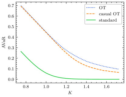
Figure 4.1: Comparison of AVaR for the option under a classical transport-type penalization (dotted), a causal transport-type penalization (dashed), and standard AVaR (solid).

Remark 4.1.

We can also consider robust risk-indifference pricing (Xu, 2006) under model uncertainty. For simplicity, we assume zero initial capital and liability. The robust risk-indifference (sell) price is the minimum price a trader will charge so that the total risk of their portfolio will not increase. It is given by

$$\inf_{H\in\mathscr{H}}\mathbf{AVaR}_{\alpha}(f+(H{\circ}X)_{N})-\inf_{H\in\mathscr{H}}\mathbf{AVaR}_{\alpha}((H{\circ}X)_{N}),$$

where $\mathscr{H}$ is the set of all predictable hedging strategies and $(H{\circ}X)_{N}=\sum_{n=1}^{N}H_{n}(X_{n}-X_{n-1})$ is the discrete stochastic integral. By Theorem 4.1, we write

$$\inf_{H\in\mathscr{H}}\mathbf{AVaR}_{\alpha}(f+(H{\circ}X)_{N})=\inf_{\lambda,\gamma\geq 0}\{L^{*}(\lambda)+\gamma+\inf_{H\in\mathscr{H}}\mathcal{E}_{\mu}[\alpha^{-1}(f+(H{\circ}X)_{N}-\gamma)^{+}-\lambda c]\}.$$

As $\alpha$ goes to 0, it is known that the risk-indifference price under $\mathrm{AVaR}_{\alpha}$ converges to the superhedging price. Under the current context, the robust superhedging price is given by

$$\rho(f):=\inf\{x:x+(H{\circ}X)_{N}\geq f-L(d_{\mathfrak{c}}(\mu,\nu))\quad\text{for some }H\in\mathscr{H}\quad\nu\text{-a.s.}\}.$$

We stress that this is a nondominated framework and is orthogonal to the setting in Bouchard and Nutz (2015). Indeed, we consider all possible reference measure $\nu\in\mathscr{P}(\mathcal{X})$ with penalization $L(d_{\mathfrak{c}}(\mu,\nu))$, whereas in Bouchard and Nutz (2015) authors considered a collection of measures which is stable under the concatenation of kernels. When $\mathcal{X}$ is compact and $f$ is continuous, we can write down pricing–hedging duality as

$$\rho(f)=\sup_{\nu\in\mathscr{P}(\mathcal{X})}\sup_{\eta\ll\nu,\eta\in\mathscr{M}(\mathcal{X})}\{E_{\eta}[f(X)]-L(d_{\mathfrak{c}}(\mu,\nu))\},$$

where $\mathscr{M}(\mathcal{X})$ denotes the set of martingale measures on $\mathcal{X}$. It is unclear if this holds under a more general setting, and we leave it for future work.

5 Distributionally robust stochastic control

Throughout this section, we assume $c(x,y)=\sum_{n=1}^{N}c_{n}(x_{n},y_{n})$. We set up the framework of distributionally robust stochastic control problems. Let $(\Omega,\mathcal{F},P)$ be a probability space, $\mathcal{X}_{1},\dots,\mathcal{X}_{N}$, $\mathcal{U}_{1},\dots,\mathcal{U}_{N}$, $\mathcal{W}_{1},\dots,\mathcal{W}_{N}$ Polish spaces, and a random variable $X_{1}$ with law $\mu_{1}\in\mathscr{P}(\mathcal{X}_{1})$. Let $g_{n}:\mathcal{X}_{1:n}\times\mathcal{U}_{n}\times\mathcal{W}_{n}\to\mathcal{X}_{n+1}$, $f_{n}:\mathcal{X}_{n}\to\mathbb{R}$, $l_{n}:\mathcal{X}_{1:n}\times\mathcal{U}_{n}\to\mathbb{R}$ be Borel measurable. We consider the non-Markovian feedback controlled system

$$\left\{\begin{aligned} X^{u}_{n+1}&=g_{n}(X^{u}_{1:n},u_{n}(X^{u}_{1:n}),w_{n}),\quad n=1,\dots,N-1,\\ X^{u}_{1}&=X_{1}\sim\mu_{1},\end{aligned}\right.$$

with the aim of minimizing

$$V=\inf_{u\in\mathscr{U}}E_{P}\Bigl{[}\sum_{n=1}^{N-1}l_{n}(\cdot,u_{n})(X^{u}_{1:n})+\sum_{n=1}^{N}f_{n}(X^{u}_{n})\Bigr{]},$$

where $w_{n}$ is a noise independent of $\sigma(X_{1:n})$ taking value in $\mathcal{W}_{n}$ for $n\in 1,\dots,N$, and $\mathscr{U}$ is the set of admissible controls given by

$$\mathscr{U}=\{u=(u_{1},\dots,u_{N-1}):u_{n}:\mathcal{X}_{1:n}\to\mathcal{U}_{n}\text{ universally measurable}\}.$$

Equivalently, with $\mu^{u}=X^{u}_{\#}P$ we can rewrite the objective functional as

$$V=\inf_{u\in\mathscr{U}}E_{\mu^{u}}\Bigl{[}\sum_{n=1}^{N-1}l_{n}(\cdot,u_{n})(X_{1:n})+\sum_{n=1}^{N}f_{n}(X_{n})\Bigr{]}.$$ (5.1)

The objective can be split into two parts: one corresponding to the cost incurred by implementing the control, and the other representing the cost of the system coming from observations. We now consider a case in which precise control on the system is achievable while the observation of the system might be subject to inaccuracies. Mathematically, we are interested in the distributionally robust stochastic control problem:

$$\mathbf{V}=\inf_{u\in\mathscr{U}}\sup_{\nu\in\mathscr{P}(\mathcal{X})}\Bigl{\{}E_{\mu}\Bigl{[}\sum_{n=1}^{N-1}l_{n}(\cdot,u_{n})(X_{n})\Bigr{]}+E_{\nu}\Bigl{[}\sum_{n=1}^{N}f_{n}(X_{n})\Bigr{]}-L(d_{\mathfrak{c}}(\mu^{u},\nu))\Bigr{\}}.$$ (5.2)

Before the discussion of the robust control problem, we take a short detour to the classical stochastic control problem. By $\mu^{u,x_{1:n}}$, we denote the law of the conditioned system $X^{u,x_{1:n}}$ under control $u$

$$\left\{\begin{aligned} X^{u,x_{1:n}}_{m+1}&=g_{m}(X^{u,x_{1:n}}_{m},u_{m}(X^{u,x_{1:n}}_{m}),w_{m}),\quad m=n,\dots,N-1,\\ X^{u,x_{1"n}}_{n}&=x_{1:n}.\end{aligned}\right.$$

We define cost-to-go functions $V_{n}:\mathcal{X}_{1:n}\to\mathbb{R}$ by

$$V_{n}(x_{1:n})=\inf_{u\in\mathscr{U}}E_{\mu^{u,x_{1:n}}}\Bigl{[}\sum_{m=n}^{N-1}l_{m}(\cdot,u_{m})(X_{1:m})+\sum_{m=n}^{N}f_{m}(X_{m})\Bigr{]}.$$

Under mild conditions, the classical dynamic programming principle yields the following Bellman equation

$$\left\{\begin{aligned} V_{n}(x_{1:n})&=\inf_{\mathfrak{u_{n}}\in\mathcal{U}_{n}}\{l_{n}(x_{1:n},\mathfrak{u_{n}})+f_{n}(x_{n})+E_{\mu^{\mathfrak{u_{n}},x_{1:n}}}[V_{n+1}(X_{n+1})]\},\\ V_{N}(x_{1:N})&=f_{N}(x_{N}).\end{aligned}\right.$$

Then one can solve the Bellman equation by backward induction and find the optimal control (if exists) by

$$u^{*}_{n}(x_{1:n})\in\arg\min_{\mathfrak{u_{n}}\in\mathcal{U}_{n}}\{l_{n}(x_{1:n},\mathfrak{u_{n}})+f_{n}(x_{n})+E_{\mu^{\mathfrak{u_{n}},x_{1:n}}}[V_{n+1}(X_{n+1})]\}.$$

However, such a dynamic programming in general does not hold for the distributionally robust control problem (5.2). The reason is that the distributionally robust control problem has a penalization term which is not compatible with the dynamic programming principle. Even in the case of $L=+\infty\mathbbm{1}_{(\delta,\infty]}$, the set $\{\nu\in\mathscr{P}(\mathcal{X}):d_{\mathfrak{c}}(\mu,\nu)\leq\delta\}$ is not stable under the concatenation of the condition probability kernels. This time inconsistency has been discovered in the context of risk averse multistage stochastic programming Shapiro (2012).

We now utilize the duality formulation and propose a feasible algorithm to solve the robust stochastic control problem (5.2). By duality, we write

$$\mathbf{V} =\inf_{\begin{subarray}{c}u\in\mathscr{U}\\ \lambda\geq 0\end{subarray}}\Biggl{\{}L^{*}(\lambda)+\sup_{\pi\in\Pi_{\mathfrak{c}}(\mu^{u},*)}E_{\pi}\Bigl{[}\sum_{n=1}^{N-1}l_{n}(\cdot,u_{n})(X_{1:n})+\sum_{n=1}^{N}\bigl{[}f_{n}(Y_{n})-\lambda c_{n}(X_{n},Y_{n})\bigr{]}\Bigr{]}\Biggr{\}}$$

$$=\inf_{\lambda\geq 0}\Biggl{\{}L^{*}(\lambda)+\inf_{u\in\mathscr{U}}\sup_{\pi\in\Pi_{\mathfrak{c}}(\mu^{u},*)}E_{\pi}\Bigl{[}\sum_{n=1}^{N-1}l_{n}(\cdot,u_{n})(X_{1:n})+\sum_{n=1}^{N}\bigl{[}f_{n}(Y_{n})-\lambda c_{n}(X_{n},Y_{n})\bigr{]}\Bigr{]}\Biggr{\}}$$

$$:=\inf_{\lambda\geq 0}\{L^{*}(\lambda)+J(\lambda)\}.$$

Once we obtain $J(\lambda)$, the outside minimization over $\lambda$ reduces to a univariate convex optimization, and hence it is efficient to find the minimizer $\lambda^{*}$. Moreover, the (sub)optimal control $u^{*}$ associated with $J(\lambda^{*})$ becomes a (sub)optimal control for the original distributionally robust control problem (5.2). Notably, to obtain the robust objective $\mathbf{V}$ under different penalties, we only need to redo the external univariate convex optimization. Thus, we shift focus to the inner optimization problem $J(\lambda)$ and show that it can be effectively solved by dynamic programming. The original time-inconsistent problem is reformulated into a sequence of time-consistent ones. In analogy to the classical case, we define the cost-to-go function $J_{n}(\lambda,\cdot):\mathcal{X}_{1:n}\to\mathbb{R}^{*}$ as

$$\qquad J_{n}(\lambda,x_{1:n})=\inf_{u\in\mathscr{U}}\sup_{\pi\in\Pi_{\mathfrak{c}}(\mu^{u,x_{1:n}},*)}E_{\pi}\Bigl{[}\sum_{m=n}^{N-1}l_{m}(\cdot,u_{m})(X_{1:m})+\sum_{m=n}^{N}\bigl{[}f_{m}(Y_{m})-\lambda c_{m}(X_{m},Y_{m})\bigr{]}\Bigr{]}.$$

Theorem 5.1.

We assume $l_{n}$, $f_{n}$ are bounded from below. Let cost-to-go function $J_{n}(\lambda,\cdot)$ be defined as above. We write $\widehat{f}_{n}(x_{n}):=\sup_{y_{n}}\{f_{n}(y_{n})-\lambda c_{n}(x_{n},y_{n})\}$. Then, we can derive $J_{n}$ from the Bellman equation

$$\left\{\begin{aligned} J_{n}(\lambda,x_{1:n})&=\inf_{\mathfrak{u}_{n}\in\mathcal{U}_{n}}\{l_{n}(x_{1:n},\mathfrak{u}_{n})+\widehat{f}_{n}(x_{n})+E_{\mu^{\mathfrak{u}_{n},x_{1:n}}}[J_{n+1}(X_{1:n+1})]\},\\ J_{N}(\lambda,x_{1:N})&=\widehat{f}_{N}(x_{N}),\end{aligned}\right.$$ (5.3)

and $J(\lambda)=\mu_{1}(J_{1})$. Furthermore, there exists an $\varepsilon$-optimal control $u^{\varepsilon}$ for any $\varepsilon>0$ satisfying

$$\sup_{\nu\in\mathscr{P}(\mathcal{X})}\Bigl{\{}E_{\mu}\Bigl{[}\sum_{n=1}^{N-1}l_{n}(\cdot,u^{\varepsilon}_{n})(X_{n})\Bigr{]}+E_{\nu}\Bigl{[}\sum_{n=1}^{N}f_{n}(X_{n})\Bigr{]}-L(d_{\mathfrak{c}}(\mu^{u^{\varepsilon}},\nu))\Bigr{\}}\leq\mathbf{V}+\varepsilon.$$

Proof.

We notice

$$J(\lambda) =\inf_{u\in\mathscr{U}}\sup_{\pi\in\Pi_{\mathfrak{c}}(\mu^{u},*)}E_{\pi}\Bigl{[}\sum_{n=1}^{N-1}l_{n}(\cdot,u_{n})(X_{1:n})+\sum_{n=1}^{N}\bigl{[}f_{n}(Y_{n})-\lambda c_{n}(X_{n},Y_{n})\bigr{]}\Bigr{]}$$

$$=\inf_{u\in\mathscr{U}}\Bigl{\{}E_{\mu^{u}}\Bigl{[}\sum_{n=1}^{N-1}l_{n}(\cdot,u_{n})(X_{1:n})\Bigr{]}+\sup_{\pi\in\Pi_{\mathfrak{c}}(\mu^{u},*)}E_{\pi}\Bigl{[}\sum_{n=1}^{N}\bigl{[}f_{n}(Y_{n})-\lambda c_{n}(X_{n},Y_{n})\bigr{]}\Bigr{]}\Bigr{\}}$$

$$=\inf_{u\in\mathscr{U}}E_{\mu^{u}}\Bigl{[}\sum_{n=1}^{N-1}l_{n}(\cdot,u_{n})(X_{1:n})+\sum_{n=1}^{N}\widehat{f}_{n}(X_{n})\Bigr{]}.$$

Therefore, $J(\lambda)$ is a classical time-consistent stochastic control problem. By Bertsekas and Shreve (1996, Propositions 8.2 and 8.3), we conclude the proof. ∎

Remark 5.1.

An alternative robust formulation involves considering the misspecification of the cost generated by control, i.e.,

$$\inf_{u\in\mathscr{U}}\sup_{\nu\in\mathscr{P}(\mathcal{X})}\Bigl{\{}E_{\nu}\Bigl{[}\sum_{n=1}^{N-1}l_{n}(\cdot,u_{n})(X_{1:n})\Bigr{]}-L(d_{\mathfrak{c}}(\mu^{u},\nu))\Bigr{\}}.$$

Although it is not covered in the current setup, it can, in some cases, be solved via the same duality result. We have chosen our formulation to provide a simple and clear presentation of how to link the duality and the dynamic programming principle.

Example 5.1.

We consider a finite horizon 1D linear quadratic stochastic control. Let $X^{u}$ follow

$$\left\{\begin{aligned} X^{u}_{n+1}&=AX^{u}_{n}+Bu_{n}(X^{u}_{n})+w_{n},\qquad n=1,\dots,N-1,\\ X^{u}_{1}&=x_{1},\end{aligned}\right.$$

with the aim of minimizing

$$V=\inf_{u\in\mathscr{U}}E_{\mu^{u}}\Bigl{[}\sum_{n=1}^{N-1}u_{n}(X_{n})^{2}+\sum_{n=1}^{N}X_{n}^{2}\Bigr{]},$$

where $w_{n}$ are i.i.d. standard normal random variables.

We take $c(x,y)=\sum_{n=1}^{N}|x_{n}-y_{n}|^{2}$ and $L=+\infty\mathbbm{1}_{(\delta,\infty]}$. From the above discussion, we derive

$$\mathbf{V}=\inf_{\lambda>1}\Bigl{\{}\delta\lambda+\inf_{u\in\mathscr{U}}E_{\mu^{u}}\Bigl{[}\sum_{n=1}^{N-1}u_{n}(X_{n})^{2}+\frac{\lambda}{\lambda-1}\sum_{n=1}^{N}X_{n}^{2}\Bigr{]}\Bigr{\}}.$$

The inner control problem is again a stochastic linear quadratic problem which can be directly solved by a difference Riccati equation.

6 Distributionally robust optimal stopping

In this section, we investigate the distributionally robust optimal stopping problem

$$\sup_{\nu\in\mathscr{P}(\mathcal{X})}\{\sup_{\tau\in\mathcal{T}_{\mathfrak{0}}}E_{\nu}[f_{\tau}(X_{1:\tau})]-L(d_{\mathfrak{c}}(\mu,\nu))\},$$ (6.1)

where $\mathcal{T}_{\mathfrak{0}}$ is the set of $(\mathcal{B}_{n}(\mathcal{X}))$–stopping times and $f_{n}:\mathcal{X}_{1:n}\to\mathbb{R}$ for $n=1,\dots,N$. We point out that

$$\nu\mapsto J(\nu):=\sup_{\tau\in\mathcal{T}_{\mathfrak{0}}}E_{\nu}[f_{\tau}(X_{1:\tau})]$$

fails to be concave in general. Hence, Theorem 3.2 is not directly applicable here. We will circumvent this issue and regain concavity by relaxing the problem to a general filtered process setting.

Before we proceed, we first give a concrete example which will shed some light on the relaxation of causal DRO. Take $\nu_{1}=\frac{1}{2}(\delta_{(0,1)}+\delta_{(0,-1)})$, $\nu_{2}=\frac{1}{2}(\delta_{(0,2)}+\delta_{(0,-2)})$, and $f_{n}(x_{1:n})=x_{n}^{2}-1$. It is direct to check

$$1+3=J(\nu_{1})+J(\nu_{2})>2J((\nu_{1}+\nu_{2})/2)=3.$$

To reconcile this, we relax the optimal stopping problem by considering richer filtrations. Heuristically, we can realize a process with law $\frac{1}{2}(\nu_{1}+\nu_{2})$ by tossing a fair coin at the first step and then follow the process with law $\nu_{1}$ or $\nu_{2}$ depending on the outcome of the coin. The value of the optimal stopping problem is exactly $\frac{1}{2}(J(\nu_{1})+J(\nu_{2}))$, if the admissible stopping time is with respect to the natural filtration augmented by the coin toss. On the other hand, if the admissible stopping time is with respect to the natural filtration, then the value is again $J((\nu_{1}+\nu_{2})/2)$. We stress that the value of the optimal stopping problem is not only determined by the law of the process but also the information flow, i.e., the filtration. In order to take all possible filtrations into account, we have to enlarge the canonical path space.

Canonical filtered process space

We formally introduce filtered processes and the canonical filtered space following Bartl et al. (2021a). A filtered process is a 5-tuple $\mathbb{X}=(\Omega^{\mathbb{X}},\mathcal{F}^{\mathbb{X}},(\mathcal{F}_{n}^{\mathbb{X}}),X,P^{\mathbb{X}})$, where $X:\Omega^{\mathbb{X}}\to\mathcal{X}$ is $(\mathcal{F}_{n}^{\mathbb{X}})$–adapted. To prevent confusion between $P^{\mathbb{X}}$ the associated law of $\mathbb{X}$ and $X_{\#}P^{\mathbb{X}}$ the law of $X$, we call $P^{\mathbb{X}}$ the filtered law of $\mathbb{X}$. The set of filtered processes is denoted by $\mathcal{FP}$. We extend the definition of causality to processes equipped with general filtrations.

Definition 6.1.

Given $\mathbb{X},\mathbb{Y}\in\mathcal{FP}$, we say a coupling $\pi\in\Pi(P^{\mathbb{X}},P^{\mathbb{Y}})\subset\mathscr{P}(\Omega^{\mathbb{X}}\times\Omega^{\mathbb{Y}})$ is causal from $\mathbb{X}$ to $\mathbb{Y}$ if for any $n\in 1,\dots,N$ and $A\in\mathcal{F}_{n}^{\mathbb{Y}}$

$$\Omega^{\mathbb{X}}\ni x\mapsto\pi_{y}(x,A)\in\mathbb{R}$$

is $\prescript{P^{\mathbb{X}}}{}{\mathcal{F}}_{n}^{\mathbb{X}}$–measurable. With a slight abuse of notation, we denote the set of causal couplings from $\mathbb{X}$ to $\mathbb{Y}$ by $\Pi_{\mathfrak{c}}(\mathbb{X},\mathbb{Y})$. The associated causal optimal transport problem is defined as

$$d_{\mathfrak{c}}(\mathbb{X},\mathbb{Y}):=\inf_{\pi\in\Pi_{\mathfrak{c}}(\mathbb{X},\mathbb{Y})}E_{\pi}[c(X,Y)].$$

While such a weak formulation encompasses all possible filtered processes of interest, it lacks a linear structure, and in particular, there is no convex structure on $\Pi_{\mathfrak{c}}(\mathbb{X},*)$. To this end, the canonical filtered space introduced in Bartl et al. (2021a) serves as a natural ambient space to encode all the information of a filtered process.

Definition 6.2.

We recursively define $\mathcal{Z}_{N}=\mathcal{X}_{N}$ and for $n=N-1,\dots,1$

$$\mathcal{Z}_{n}=\mathcal{Z}_{n}^{-}\times\mathcal{Z}_{n}^{+}:=\mathcal{X}_{n}\times\mathscr{P}(\mathcal{Z}_{n+1}).$$

The canonical filtered space is the tuple $(\mathcal{Z},\mathcal{B}(\mathcal{Z}),(\mathcal{B}_{n}(\mathcal{Z})),Z^{-})$, where $\mathcal{Z}=\mathcal{Z}_{1:N}$, $\mathcal{B}_{n}(\mathcal{Z})=\sigma(Z_{1:n})$, and $Z^{-}:\mathcal{Z}\to\mathcal{X}$ is the projection map. There is a natural embedding from $\mathcal{X}$ to $\mathcal{Z}$. We will not distinguish $\mathcal{X}$ and $\mathcal{Z}^{-}$ as a subspace of $\mathcal{Z}$.

Definition 6.3.

For a given filtered process $\mathbb{X}=(\Omega^{\mathbb{X}},\mathcal{F}^{\mathbb{X}},(\mathcal{F}_{n}^{\mathbb{X}}),X,P^{\mathbb{X}})$, the associated information process $I^{\mathbb{X}}$ is given recursively by $I_{N}^{\mathbb{X}}:=X_{N}$ and

$$I_{n}^{\mathbb{X}}:=(X_{n},\operatorname{Law}(I_{n+1}^{\mathbb{X}}|\mathcal{F}_{n}^{\mathbb{X}})).$$

We define a relation ‘$\sim$’ on $\mathcal{FP}$ by

$$\mathbb{X}\sim\mathbb{Y}\quad\text{if and only if}\quad(I^{\mathbb{X}})_{\#}P^{\mathbb{X}}=(I^{\mathbb{Y}})_{\#}P^{\mathbb{Y}}.$$

The canonical representation of $\mathbb{X}$ is given by $\bar{\mathbb{X}}=(\mathcal{Z},\mathcal{B}(\mathcal{Z}),\mathcal{B}_{n}(\mathcal{Z}),Z^{-},P^{\bar{\mathbb{X}}})$, where $P^{\bar{\mathbb{X}}}=(I^{\mathbb{X}})_{\#}P^{\mathbb{X}}\in\mathscr{P}(\mathcal{Z})$. Indeed, one can show $P^{\bar{\mathbb{X}}}=(I^{\bar{\mathbb{X}}})_{\#}P^{\bar{\mathbb{X}}}$.

The following proposition shows that it suffices to consider the canonical filtered processes.

Proposition 6.1.

For any $\mathbb{X},\mathbb{Y}\in\mathcal{FP}$, we have

• $\mathbb{X}\sim\mathbb{Y}$ if and only if $(I_{1}^{\mathbb{X}})_{\#}P^{\mathbb{X}}=(I_{1}^{\mathbb{Y}})_{\#}P^{\mathbb{Y}}$.

• $d_{\mathfrak{c}}(X,Y)=d_{\mathfrak{c}}(\bar{X},\bar{Y})$ and $d_{\mathfrak{bc}}(X,Y)=d_{\mathfrak{bc}}(\bar{X},\bar{Y})$.

• There exists universally measurable $F:\mathcal{Z}_{1}\to\mathbb{R}$ such that

  $$\sup_{\tau\in\mathcal{T}^{\mathbb{X}}}E_{P^{\mathbb{X}}}[f_{\tau}(X_{1:\tau})]=\sup_{\tau\in\mathcal{T}}E_{P^{\bar{\mathbb{X}}}}[f_{\tau}(Z^{-}_{1:\tau})]=E_{P^{\bar{\mathbb{X}}}_{1}}[F(Z_{1})],$$

  where $\mathcal{T}$ is the set of $(\mathcal{F}_{n}^{\mathbb{X}})$–stopping times and $\mathcal{T}$ is the set of $(\mathcal{B}_{n}(\mathcal{Z}))$–stopping times.

Proof.

The first statement follows from (Bartl et al., 2021a, Lemma 3.3), and the second statement follows from (Bartl et al., 2021a, Lemma 3.9). The last statement follows from Snell envelope theorem. Define recursively $f_{N}(z_{1:N}):=f(z_{1:N}^{-})$ and for $n=N-1,\dots,1$

$$F_{n}(z_{1:n})=\max\{f_{n}(z_{1:n}^{-}),z_{n}^{+}(F_{n+1}(z_{1:n},\cdot))\}.$$

Then $F=F_{1}$ is the desired function. ∎

In the sequel, we assume any filtered process is chosen as its canonical representation. Let $(\mathcal{W},\mathcal{B}(\mathcal{W}),(\mathcal{B}_{n}(\mathcal{W})),\mathcal{W}^{-})$ be a copy of the canonical filtered space, and by $P,Q$ we denote the filtered law of $\mathbb{X},\mathbb{Y}$ respectively. With a slight abuse of notation, we denote the set of the filtered laws of canonical filtered processes by

$$\mathcal{FP}=\{P\in\mathscr{P}(\mathcal{Z}):P(\mathop{}\mathopen{\mathrm{missing}}{d}z)=P_{1}(\mathop{}\mathopen{\mathrm{missing}}{d}z_{1})z_{1}^{+}(\mathop{}\mathopen{\mathrm{missing}}{d}z_{2})\dots z_{N-1}^{+}(\mathop{}\mathopen{\mathrm{missing}}{d}z_{N})\},$$

equipped with the weak topology as a subset of $\mathscr{P}(\mathcal{Z})$.

As a preparation for the duality of relaxed causal DRO, we present a new dynamic programming principle for causal optimal transport between filtered processes.

Theorem 6.2.

We assume $c$ is lower semi-analytic, bounded from below, and semi-separable, i.e., $c(z^{-},w^{-})=\sum_{n=1}^{N}c_{n}(z_{n}^{-},w_{1:n}^{-})$. We recursively define $C_{n}:\mathscr{P}(\mathcal{Z}_{n})\times\mathcal{W}_{1:n}\to\mathbb{R}$. Let $C_{N}=0$, and for $n=N-1,\dots,1$

$$C_{n}(\gamma,w_{1:n}):=\inf_{\pi\in\Pi(\gamma(z_{n}^{+}),w_{n}^{+})}E_{\pi}[c_{n+1}(Z_{n+1}^{-},w^{-}_{1:n},W_{n+1}^{-})+C_{n+1}(\pi_{z_{n+1}}(W_{n+1}),w_{1:n},W_{n+1})].$$

Here, $\gamma(z_{n}^{+})\in\mathscr{P}(Z_{n+1})$ is the ‘expectation’ of $Z_{n}^{+}$ with law $\gamma$. Then, we can rewrite the causal optimal transport problem as a weak optimal transport problem

$$d_{\mathfrak{c}}(\mathbb{X},\mathbb{Y}) =\inf_{\pi\in\Pi(P_{1},Q_{1})}E_{\pi}[c_{1}(Z_{1}^{-},W_{1}^{-})+C_{1}(\pi_{z_{1}}(W_{1}),W_{1})]$$

$$=\inf_{\pi\in\Pi(P_{1},Q_{1})}E_{\pi}[C(\pi_{z_{1}}(W_{1}),W_{1})],$$

where $C(\gamma,w_{1}):=\gamma(c_{1}(\cdot,w_{1}^{-}))+C_{1}(\gamma,w_{1})$. In particular, $C_{n}$ and $C$ are convex in the first argument and jointly lower semi-analytic. Furthermore, if $\mathcal{Z}$ is compact and $c$ is lower semi-continuous, then $C$ is lower semi-continuous.

Remark 6.4.

The above extends the dynamic programming principle in Backhoff-Veraguas et al. (2017, Theorem 4.2) to general filtered processes. Notably, we do not require the source process $\mathbb{X}$ to be Markovian.

Proof.

The measurability part follows from similar arguments in Backhoff-Veraguas et al. (2017, Theorem 4.2). For brevity, we skip the discussion and assume the well-posedness of all integrations appearing in the proof.

Let $\pi\in\Pi_{\mathfrak{c}}(\mathbb{X},\mathbb{Y})$. We write $\gamma^{n}:\mathcal{W}_{1:n-1}\to\mathscr{P}(\mathcal{Z}_{n}\times\mathcal{W}_{n})$ as the disintegration kernel

$$\pi(\mathop{}\mathopen{\mathrm{missing}}{d}z_{n},\mathop{}\mathopen{\mathrm{missing}}{d}w_{1:n}) =Q(\mathop{}\mathopen{\mathrm{missing}}{d}w_{1:n-1})\gamma^{n}(w_{1:n-1},\mathop{}\mathopen{\mathrm{missing}}{d}z_{n},\mathop{}\mathopen{\mathrm{missing}}{d}w_{n})$$

$$=Q(\mathop{}\mathopen{\mathrm{missing}}{d}w_{1:n-1})\gamma^{n}(w_{1:n-1},\mathop{}\mathopen{\mathrm{missing}}{d}w_{n})\gamma^{n}_{z_{n}}(w_{1:n},\mathop{}\mathopen{\mathrm{missing}}{d}z_{n}).$$

Similar to Bartl et al. (2021a, Lemma A.1), we have $\pi$ is causal if and only if it has successive disintegration kernels

$$\pi(\mathop{}\mathopen{\mathrm{missing}}{d}z,\mathop{}\mathopen{\mathrm{missing}}{d}w) =\pi_{1}(\mathop{}\mathopen{\mathrm{missing}}{d}z_{1},\mathop{}\mathopen{\mathrm{missing}}{d}w_{1})\pi_{2}(z_{1},w_{1},\mathop{}\mathopen{\mathrm{missing}}{d}z_{2},\mathop{}\mathopen{\mathrm{missing}}{d}w_{2})\cdots\pi_{N}(z_{1:N-1},w_{1:N-1},\mathop{}\mathopen{\mathrm{missing}}{d}z_{N},\mathop{}\mathopen{\mathrm{missing}}{d}w_{N})$$

satisfying for any $n=2,\dots,N$ and $\pi$-almost surely $z_{1:n-1},w_{1:n-1}$

$$\pi_{n}(z_{1:n-1},w_{1:n-1},\mathop{}\mathopen{\mathrm{missing}}{d}z_{n},\mathop{}\mathopen{\mathrm{missing}}{d}w_{n})\in\Pi(z_{n-1}^{+},*).$$

Therefore, for any causal coupling $\pi$ we have $\gamma^{1}\in\Pi(P_{1},Q_{1})$ and for $n=2,\dots,N$

$$\gamma^{n}(w_{1:n-1},\mathop{}\mathopen{\mathrm{missing}}{d}z_{n},\mathop{}\mathopen{\mathrm{missing}}{d}w_{n}) =\gamma^{n-1}_{z_{n-1}}(w_{1:n-1},\mathop{}\mathopen{\mathrm{missing}}{d}z_{n-1})\cdots\gamma^{1}_{z_{1}}(w_{1},\mathop{}\mathopen{\mathrm{missing}}{d}z_{1})\pi_{n}(z_{1:n-1},w_{1:n-1},\mathop{}\mathopen{\mathrm{missing}}{d}z_{n},\mathop{}\mathopen{\mathrm{missing}}{d}w_{n})$$

$$\in\Pi(\gamma^{n-1}_{z_{n-1}}(w_{1:n-1})(z_{n-1}^{+}),w_{n-1}^{+}).$$

On the other hand, we write

$$\Gamma:=\{(\gamma^{1},\dots,\gamma^{N}):\gamma^{1}\in\Pi(P_{1},Q_{1}),\gamma^{n}(\cdot)\in\Pi(\gamma^{n-1}_{z_{n-1}}(\cdot)(z_{n-1}^{+}),w_{n-1}^{+})\text{ for }2\leq n\leq N\}.$$

For any $(\gamma^{1},\dots,\gamma^{N})\in\Gamma$, we construct

$$\pi(\mathop{}\mathopen{\mathrm{missing}}{d}z,\mathop{}\mathopen{\mathrm{missing}}{d}w):=\gamma^{1}(\mathop{}\mathopen{\mathrm{missing}}{d}z_{1},\mathop{}\mathopen{\mathrm{missing}}{d}w_{1})z^{+}_{1}(\mathop{}\mathopen{\mathrm{missing}}{d}z_{2})\gamma^{2}_{w_{2}}(z_{2},w_{1},\mathop{}\mathopen{\mathrm{missing}}{d}w_{2})\cdots z_{N-1}^{+}(\mathop{}\mathopen{\mathrm{missing}}{d}z_{N})\gamma^{N}_{w_{N}}(z_{N},w_{1:N-1},\mathop{}\mathopen{\mathrm{missing}}{d}w_{N}).$$

It is direct to check such $\pi$ belongs to $\Pi_{\mathfrak{c}}(\mathbb{X},\mathbb{Y})$. Hence, we construct a bijection between $\Gamma$ and $\Pi_{\mathfrak{c}}(\mathbb{X},\mathbb{Y})$. This implies

$$\inf_{\pi\in\Pi_{\mathfrak{c}}(\mathbb{X},\mathbb{Y})}E_{\pi}[c(Z^{-},W^{-})] =\inf_{\pi\in\Pi_{\mathfrak{c}}(\mathbb{X},\mathbb{Y})}E_{\pi}[c_{1}+E_{\pi}[c_{2}+\cdots+E_{\pi}[c_{N}|\mathcal{B}_{N-1}(\mathcal{W})]\cdots|\mathcal{B}_{1}(\mathcal{W})]]$$

$$=\inf_{\pi\in\Pi_{\mathfrak{c}}(\mathbb{X},\mathbb{Y})}\gamma^{1}(c_{1}+\gamma^{2}(c_{2}+\cdots+\gamma^{N}(c_{N})))$$

$$=\inf_{(\gamma^{1},\dots,\gamma^{N})\in\Gamma}\gamma^{1}(c_{1}+\gamma^{2}(c_{2}+\cdots+\gamma^{N}(c_{N})))$$

$$=\inf_{\pi\in\Pi(P_{1},Q_{1})}E_{\pi}[C(\pi_{z_{1}}(W_{1}),W_{1})].$$

The lower semi-continuity of $C$ follows from the compactness of $\mathcal{Z}$ and the lower semi-continuity of $c$ by Bertsekas and Shreve (1996, Proposition 7.33). ∎

Relaxed causal DRO

We focus on the relaxed distributionally robust optimal stopping

$$\sup_{\mathbb{Y}\in\mathcal{FP}}\{\sup_{\tau\in\mathcal{T}}E_{Q}[f_{\tau}(Z^{-}_{1:\tau})]-L(d_{\mathfrak{c}}(\mathbb{X},\mathbb{Y}))\},$$ (6.2)

or more generally the relaxed causal DRO

$$\sup_{\mathbb{Y}\in\mathcal{FP}}\{E_{Q}[F(Z_{1})]-L(d_{\mathfrak{c}}(\mathbb{X},\mathbb{Y}))\}.$$

Assumption 6.1.

We assume that $P\in\mathcal{FP}\subset\mathscr{P}(\mathcal{Z})$, $L:\mathbb{R}^{*}\to\mathbb{R}^{*}$ is a nondecreasing closed proper convex function with $L(0)=0$ and $L(+\infty)=+\infty$, $c:\mathcal{Z}^{-}\times\mathcal{W}^{-}\to\mathbb{R}^{*}$ is lower semi-analytic and non-negative with $c(z^{-},w^{-})=0$ if and only if $z^{-}=w^{-}$, and $F:\mathcal{W}_{1}\to\mathbb{R}$ is universally measurable with $|E_{Q}[F]|\leq K(d_{\mathfrak{c}}(\mathbb{X},\mathbb{Y})+1)$ for some constant $K>0$ and any $\mathbb{Y}$ with filtered law $Q$.

Theorem 6.3.

Under Assumption 6.1, we have

$$\sup_{\mathbb{Y}\in\mathcal{FP}}\{E_{Q}[F(Z_{1})]-L(d_{\mathfrak{c}}(\mathbb{X},\mathbb{Y}))\}=\inf_{\lambda\geq 0}\{L^{*}(\lambda)+\mathcal{E}_{P}^{\mathfrak{c}}[F-\lambda c]\},$$ (6.3)

where $\mathcal{E}_{P}^{\mathfrak{c}}[F-\lambda c]=\sup_{\pi\in\Pi_{\mathfrak{c}}(P,\mathcal{FP})}E_{\pi}[F(W_{1})-\lambda c(Z^{-},W^{-})]$. Moreover, if $c$ is semi-separable in the sense that $c(z^{-},w^{-})=\sum_{n=1}^{N}c_{n}(z_{n}^{-},w_{1:n}^{-})$, then

$$\mathcal{E}_{P}^{\mathfrak{c}}[F-\lambda c]=\sup_{\pi\in\Pi(P_{1},*)}E_{\pi}[F(W_{1})-\lambda C(\pi_{z_{1}}(W_{1}),W_{1})],$$ (6.4)

where $C:\mathscr{P}(\mathcal{Z}_{1})\times\mathcal{W}_{1}\to\mathbb{R}$ is given in Theorem 6.2 and $\pi(\mathop{}\mathopen{\mathrm{missing}}{d}z_{1},\mathop{}\mathopen{\mathrm{missing}}{d}w_{1})=\pi_{w_{1}}(\mathop{}\mathopen{\mathrm{missing}}{d}w_{1})\pi_{z_{1}}(w_{1},\mathop{}\mathopen{\mathrm{missing}}{d}z_{1})$. Additionally, if $\mathcal{X}$ is compact (equivalently, $\mathcal{Z}$ is compact), $F$ is upper semi-continuous, and $c$ is lower semi-continuous, then

$$\mathcal{E}_{P}^{\mathfrak{c}}[F-\lambda c]=\inf_{\varphi\in\mathcal{C}_{b}(\mathcal{Z}_{1})}\{P_{1}(\varphi)+\sup_{\gamma\in\mathscr{P}(\mathcal{Z}_{1})}\{\psi(\gamma)-\gamma(\varphi)\}\},$$ (6.5)

where $\psi(\gamma)=\sup_{w_{1}\in\mathcal{W}_{1}}\{F(w_{1})-\lambda C(\gamma,w_{1})\}$.

Remark 6.5.

As mentioned in Backhoff-Veraguas et al. (2017), we do not expect the semi-separability assumption on $c$ can be relaxed. It is because (6.4) relies on a recursive formulation of the causal optimal transport problem which reduces the causal optimal transport to a weak optimal transport problem. A general cost does not admit such a reformulation.

Remark 6.6.

We assume the compactness of $\mathcal{Z}$ in (6.5) to satisfy the conditions for the minimax theorem of Fan (1953). We remark that, even without the compactness assumption, $C$ is lower semi-continuous if $c$ is separable and lower semi-continuous. However, it remains open if the duality holds without the compactness assumption on $\mathcal{Z}$.

Proof.

Since $\mathcal{FP}$ is convex, by Remark 3.1 we derive (6.3). We highlight the fundamental distinct between $\mathcal{E}_{P}^{\mathfrak{c}}$ and $\mathcal{E}_{\mu}$ as derived in (3.2). The difference arises from the constraint on the second marginal of the coupling. To show (6.4), we utilize a weak optimal transport reformulation for causal optimal transport. By Theorem 6.2 there exists $C:\mathscr{P}(\mathcal{Z}_{1})\times\mathcal{W}_{1}\to\mathbb{R}$ such that

$$\mathcal{E}_{P}^{\mathfrak{c}}[F-\lambda c] =\sup_{Q\in\mathcal{FP}}\sup_{\pi\in\Pi_{\mathfrak{c}}(P,Q)}E_{\pi}[F(W_{1})-\lambda c(Z^{-},W^{-})]$$

$$=\sup_{Q\in\mathcal{FP}}\sup_{\pi\in\Pi(P_{1},Q_{1})}E_{\pi}[F(W_{1})-\lambda C(\pi_{z_{1}}(W_{1}),W_{1})]$$

$$=\sup_{\pi\in\Pi(P_{1},*)}E_{\pi}[F(W_{1})-\lambda C(\pi_{z_{1}}(W_{1}),W_{1})].$$

Now, we assume the canonical filtered space $\mathcal{Z}$ is compact, $F$ is upper semi-continuous, and $c$ is lower semi-continuous. As pointed out in Backhoff-Veraguas et al. (2019), we can embed coupling $\pi\in\mathscr{P}(\mathcal{Z}_{1},\mathcal{W}_{1})$ into a nested space $\mathscr{P}(\mathscr{P}(\mathcal{Z}_{1})\times\mathcal{W}_{1})$ by

$$\mathscr{P}(\mathcal{Z}_{1},\mathcal{W}_{1})\ni\pi\mapsto[(z_{1},w_{1})\mapsto(\pi_{z_{1}}(w_{1}),w_{1})]_{\#}\pi\in\mathscr{P}(\mathscr{P}(\mathcal{Z}_{1})\times\mathcal{W}_{1}).$$

This yields

$$\mathcal{E}_{P}^{\mathfrak{c}}[F-\lambda c]\leq\sup_{\begin{subarray}{c}\varpi\in\mathscr{P}(\mathscr{P}(\mathcal{Z}_{1})\times\mathcal{W}_{1})\\ \varpi(\gamma)=P_{1}\end{subarray}}E_{\varpi}[F(W_{1})-\lambda C(\gamma,W_{1})]$$

On the other hand, $C(\cdot,w_{1})$ is convex by Theorem 6.2. Hence, for any $\varpi\in\mathscr{P}(\mathscr{P}(\mathcal{Z}_{1})\times\mathcal{W}_{1})$ with $\varpi(\gamma)=P_{1}$ we have

$$E_{\varpi}[F(W_{1})-\lambda C(\gamma,W_{1})]\leq E_{\varpi}[F(W_{1})-\lambda C(\varpi_{\gamma}(W_{1})(\gamma),W_{1})]\leq\mathcal{E}_{P}^{\mathfrak{c}}[F-\lambda c].$$

Hence, we obtain

$$\mathcal{E}_{P}^{\mathfrak{c}}[F-\lambda c] =\sup_{\begin{subarray}{c}\varpi\in\mathscr{P}(\mathscr{P}(\mathcal{Z}_{1})\times\mathcal{W}_{1})\\ \varpi(\gamma)=P_{1}\end{subarray}}E_{\varpi}[F(W_{1})-\lambda C(\gamma,W_{1})]$$

$$=\sup_{\varpi\in\mathscr{P}(\mathscr{P}(\mathcal{Z}_{1})\times\mathcal{W}_{1})}\inf_{\varphi\in\mathcal{C}_{b}(\mathcal{Z}_{1})}\{P_{1}(\varphi)+E_{\varpi}[F(W_{1})-\lambda C(\gamma,W_{1})-\gamma(\varphi)]\}.$$

Since $c$ is lower semi-continuous and $\mathcal{Z}$ is compact, we derive $C$ is lower-semi continuous from Theorem 6.2. This implies

$$(\varpi,\varphi)\mapsto P_{1}(\varphi)+E_{\varpi}[F(W_{1})-\lambda C(\gamma,W_{1})-\gamma(\varphi)]$$

is concave and upper semi-continuous in $\varpi$ and convex in $\varphi$. Combing this with the fact that $\mathscr{P}(\mathscr{P}(\mathcal{Z}_{1})\times\mathcal{W}_{1})$ is compact, we apply Fan (1953, Theorem 2) and obtain

$$\mathcal{E}_{P}^{\mathfrak{c}}[F-\lambda c] =\inf_{\varphi\in\mathcal{C}_{b}(\mathcal{Z}_{1})}\sup_{\varpi\in\mathscr{P}(\mathscr{P}(\mathcal{Z}_{1})\times\mathcal{W}_{1})}\{P_{1}(\varphi)+E_{\varpi}[F(W_{1})-\lambda C(\gamma,W_{1})-\gamma(\varphi)]\}$$

$$=\inf_{\varphi\in\mathcal{C}_{b}(\mathcal{Z}_{1})}\{P_{1}(\varphi)+\sup_{\gamma\in\mathscr{P}(\mathcal{Z}_{1})}\{\psi(\gamma)-\gamma(\varphi)\}\}.$$

∎

We also consider the relaxed problem under a bicausal transport penalization.

Theorem 6.4.

Under Assumption 6.1, we have

$$\sup_{\mathbb{Y}\in\mathcal{FP}}\{E_{Q}[F(Z_{1})]-L(d_{\mathfrak{bc}}(\mathbb{X},\mathbb{Y}))\}=\inf_{\lambda\geq 0}\{L^{*}(\lambda)+\mathcal{E}_{P}^{\mathfrak{bc}}[F-\lambda c]\},$$ (6.6)

where $\mathcal{E}_{P}^{\mathfrak{bc}}[F-\lambda c]=\sup_{\pi\in\Pi_{\mathfrak{bc}}(P,\,\mathcal{FP})}E_{\pi}[F(W_{1})-\lambda c(Z^{-},W^{-})]$. Furthermore, there exists $C:\mathcal{Z}_{1}\times\mathcal{W}_{1}\to\mathbb{R}$ such that

$$\mathcal{E}_{P}^{\mathfrak{bc}}[F-\lambda c] =\sup_{\pi\in\Pi(P_{1},*)}E_{\pi}[F(W_{1})-\lambda C(Z_{1},W_{1})]$$

$$=E_{P_{1}}[\sup_{w_{1}\in\mathcal{W}_{1}}\{F(w_{1})-\lambda C(Z_{1},w_{1})\}].$$

Proof.

Following the proof of Theorem 3.2, to show (6.6) it suffices to show the convexity of the bicausal cost $d_{\mathfrak{bc}}(\mathbb{X},\cdot)$. As mentioned above, $\Pi_{\mathfrak{bc}}(\mathbb{X},*)$ is not a convex set. Hence, the convexity of $d_{\mathfrak{bc}}(\mathbb{X},\cdot)$ does not follow from the same line of argument as the causal case. Instead, we reformulate the bicausal optimal transport problem as a classical optimal transport problem which has been shown in Bartl et al. (2021a, Theorem 3.10). We adapt their result to the current setting. Define $C_{N}=c$, and for $n=N-1,\dots,1$

$$C_{n}(z_{1:n-1}^{-},z_{n},w_{1:n-1}^{-},w_{n})=\inf_{\pi\in\Pi(z_{n}^{+},w_{n}^{+})}E_{\pi}[C_{n+1}(z_{1:n}^{-},Z_{n+1},w_{1:n}^{-},W_{n+1})].$$

Then, we obtain

$$d_{\mathfrak{bc}}(\mathbb{X},\mathbb{Y}) =\inf_{\pi\in\Pi(P_{1},Q_{1})}E_{\pi}[C_{1}(Z_{1},W_{1})].$$

This implies the convexity of $d_{\mathfrak{bc}}(\mathbb{X},\cdot)$. The rest of the proof is a direct application of Theorem 3.2 in the static setting. ∎

Further discussion on plain processes

It is obvious that the value of (6.1) is not greater than the value of (6.2). We are interested in the case when the two values agree. To this end, by $\mathcal{FP}_{\mathfrak{0}}$ we denote the set of plain processes defined as

$$\mathcal{FP}_{\mathfrak{0}}:=\{\mathbb{X}\in\mathcal{FP}:(\Omega^{\mathbb{X}},\mathcal{F}^{\mathbb{X}},(\mathcal{F}_{n}^{\mathbb{X}}),X,P^{\mathbb{X}})\sim(\Omega^{\mathbb{X}},\mathcal{F}^{\mathbb{X}},(\sigma(X_{1:n})),X,P^{\mathbb{X}})\}.$$

For simplicity, we denote the set of the filtered laws of canonical plain processes by $\mathcal{FP}_{\mathfrak{0}}\subset\mathcal{FP}\subset\mathscr{P}(\mathcal{Z})$.

Theorem 6.5.

Suppose that Assumption 6.1 holds. We further assume that $\mathcal{X}$ has no isolated points, and $F:\mathcal{Z}_{1}\to\mathbb{R}$, $c:\mathcal{Z}^{-}\times\mathcal{W}^{-}\to\mathbb{R}$ are continuous and bounded. Then, the value of the relaxed problem agrees with the value of the original problem, i.e.,

$$\sup_{\mathbb{Y}\in\mathcal{FP}}\{E_{Q}[F(Z_{1})]-L(d_{\mathfrak{c}}(\mathbb{X},\mathbb{Y}))\}=\sup_{\mathbb{Y}\in\mathcal{FP}_{\mathfrak{0}}}\{E_{Q}[F(Z_{1})]-L(d_{\mathfrak{c}}(\mathbb{X},\mathbb{Y}))\},$$

and

$$\sup_{\mathbb{Y}\in\mathcal{FP}}\{E_{Q}[F(Z_{1})]-L(d_{\mathfrak{bc}}(\mathbb{X},\mathbb{Y}))\}=\sup_{\mathbb{Y}\in\mathcal{FP}_{\mathfrak{0}}}\{E_{Q}[F(Z_{1})]-L(d_{\mathfrak{bc}}(\mathbb{X},\mathbb{Y}))\}.$$

Proof.

Since $\mathcal{X}$ has no isolated points, Bartl et al. (2021a, Theorem 5.5) implies $\mathcal{FP}_{\mathfrak{0}}$ is dense in $\mathcal{FP}$. Moreover, since $c$ is continuous and bounded, Eckstein and Pammer (2022, Theorem 3.6) implies $d_{\mathfrak{c}}(\mathbb{X},\cdot)$ and $d_{\mathfrak{bc}}(\mathbb{X},\cdot)$ are continuous. Hence, for any $\mathbb{Y}\in\mathcal{FP}$ there exists $\mathbb{Y}^{n}\in\mathcal{FP}_{\mathfrak{0}}$ such that $E_{Q^{n}}[F(Z_{1})]\to E_{Q}[F(Z_{1})]$, $d_{\mathfrak{c}}(\mathbb{X},\mathbb{Y}^{n})\nearrow d_{\mathfrak{c}}(\mathbb{X},\mathbb{Y})$, and $d_{\mathfrak{bc}}(\mathbb{X},\mathbb{Y}^{n})\nearrow d_{\mathfrak{bc}}(\mathbb{X},\mathbb{Y})$. This concludes the proof.

∎

Corollary 6.6.

Let $c$ and $f_{n}:\mathcal{X}_{1:n}\to\mathbb{R}$ be continuous and bounded for $n=1,\dots,N$. We further assume that $\mathcal{X}$ has no isolated points. Let $\mathbb{X}$ be a plain filtered process with law $\mu$. Then, we have

$$\sup_{\nu\in\mathscr{P}(\mathcal{X})}\{\sup_{\tau\in\mathcal{T}_{\mathfrak{0}}}E_{\nu}[f_{\tau}(X_{1:\tau})]-L(d_{\mathfrak{c}}(\mu,\nu))\}=\sup_{\mathbb{Y}\in\mathcal{FP}}\{\sup_{\tau\in\mathcal{T}}E_{Q}[f_{\tau}(Z^{-}_{1:\tau})]-L(d_{\mathfrak{c}}(\mathbb{X},\mathbb{Y}))\},$$

and

$$\sup_{\nu\in\mathscr{P}(\mathcal{X})}\{\sup_{\tau\in\mathcal{T}_{\mathfrak{0}}}E_{\nu}[f_{\tau}(X_{1:\tau})]-L(d_{\mathfrak{bc}}(\mu,\nu))\}=\sup_{\mathbb{Y}\in\mathcal{FP}}\{\sup_{\tau\in\mathcal{T}}E_{Q}[f_{\tau}(Z^{-}_{1:\tau})]-L(d_{\mathfrak{bc}}(\mathbb{X},\mathbb{Y}))\}.$$

Proof.

Define recursively $F_{N}(z):=f_{N}(z^{-})$, for $n=N-1,\dots,1$

$$F_{n}(z_{1:n})=\max\{f_{n}(z_{1:n}^{-}),z_{n}^{+}(F_{n+1}(z_{1:n},\cdot))\}.$$

By Snell envelope theorem, we have

$$\sup_{\tau\in\mathcal{T}}E_{Q}[f_{\tau}(Z^{-}_{1:\tau})]=E_{Q}[F_{1}(Z_{1})].$$

We prove $F_{n}$ are continuous and bounded by induction. It suffices to show $z_{1:n}\mapsto z_{n}^{+}(F_{n+1}(z_{1:n},\cdot))$ is continuous which follows directly from Prokhorov’s theorem. By Theorem 6.5, we conclude the proof. ∎

Remark 6.7.

In particular, if we take $f_{n}=-1-\|f_{N}\|_{\infty}$, then $\tau=N$ is an optimal stopping time and

$$\sup_{\tau\in\mathcal{T}}E_{Q}[f_{\tau}(Z^{-}_{1:\tau})]=E_{Q}[f_{N}(Z^{-}_{1:N})].$$

Hence, we can equip any filtered process $\mathbb{Y}$ with the richest filtration while keeping the same value of the optimal stopping. This implies the value of the relaxed causal problem agrees with the value of the relaxed bicausal problem. Combing this with the above corollary, we conclude the value of the original causal problem agrees with the value of the original bicausal problem. This extends Corollary 3.3 to abstract polish spaces.

References

- Acciaio et al. (2020) B. Acciaio, J. Backhoff-Veraguas, and A. Zalashko. Causal optimal transport and its links to enlargement of filtrations and continuous-time stochastic optimization. Stochastic Processes and their Applications, 130(5):2918–2953, May 2020.
- Aldous (1981) D. Aldous. Weak convergence and the general theory of processes. Incomplete draft of monograph, July 1981.
- Backhoff-Veraguas et al. (2017) J. Backhoff-Veraguas, M. Beiglböck, Y. Lin, and A. Zalashko. Causal transport in discrete time and applications. SIAM J. Optim., 27(4):2528–2562, Jan. 2017.
- Backhoff-Veraguas et al. (2019) J. Backhoff-Veraguas, M. Beiglböck, and G. Pammer. Existence, duality, and cyclical monotonicity for weak transport costs. Calculus of Variations and Partial Differential Equations, 58(6):203, 2019.
- Backhoff-Veraguas et al. (2020a) J. Backhoff-Veraguas, D. Bartl, M. Beiglböck, and M. Eder. Adapted Wasserstein distances and stability in mathematical finance. Finance Stoch, 24(3):601–632, July 2020a.
- Backhoff-Veraguas et al. (2020b) J. Backhoff-Veraguas, D. Bartl, M. Beiglböck, and M. Eder. All adapted topologies are equal. Probab. Theory Relat. Fields, 178(3-4):1125–1172, Dec. 2020b.
- Backhoff-Veraguas et al. (2020c) J. Backhoff-Veraguas, M. Beiglböck, M. Eder, and A. Pichler. Fundamental properties of process distances. Stochastic Processes and their Applications, 130(9):5575–5591, Sept. 2020c.
- Backhoff-Veraguas et al. (2022) J. Backhoff-Veraguas, S. Källblad, and B. A. Robinson. Adapted Wasserstein distance between the laws of SDEs, Sept. 2022. arXiv:2209.03243.
- Bai et al. (2023) X. Bai, G. He, Y. Jiang, and J. Obłój. Wasserstein distributional robustness of neural networks. In Advances in Neural Information Processing Systems. Curran Associates, Inc., Dec. 2023.
- Bartl and Wiesel (2023) D. Bartl and J. Wiesel. Sensitivity of multi-period optimization problems in adapted Wasserstein distance, Aug. 2023. SIAM J. Financial Math. (forthcoming).
- Bartl et al. (2020) D. Bartl, S. Drapeau, and L. Tangpi. Computational aspects of robust optimized certainty equivalents and option pricing. Mathematical Finance, 30(1):287–309, 2020.
- Bartl et al. (2021a) D. Bartl, M. Beiglböck, and G. Pammer. The Wasserstein space of stochastic processes, Apr. 2021a. arXiv:2104.14245.
- Bartl et al. (2021b) D. Bartl, S. Drapeau, J. Obłój, and J. Wiesel. Sensitivity analysis of Wasserstein distributionally robust optimization problems. Proc. R. Soc. A., 477(2256):20210176, Dec. 2021b.
- Bartl et al. (2023) D. Bartl, A. Neufeld, and K. Park. Sensitivity of robust optimization problems under drift and volatility uncertainty, 2023. arXiv:2311.11248.
- Bertsekas and Shreve (1996) D. Bertsekas and S. E. Shreve. Stochastic Optimal Control: The Discrete-Time Case. Athena Scientific, Dec. 1996.
- Bion–Nadal and Talay (2019) J. Bion–Nadal and D. Talay. On a Wasserstein-type distance between solutions to stochastic differential equations. Ann. Appl. Probab., 29(3), June 2019.
- Blanchet and Murthy (2019) J. Blanchet and K. Murthy. Quantifying distributional model risk via optimal transport. Mathematics of OR, 44(2):565–600, May 2019.
- Blanchet et al. (2019) J. Blanchet, Y. Kang, and K. Murthy. Robust wasserstein profile inference and applications to machine learning. Journal of Applied Probability, 56(3):830–857, 2019.
- Blanchet et al. (2022) J. Blanchet, L. Chen, and X. Y. Zhou. Distributionally robust mean-variance portfolio selection with wasserstein distances. Management Science, 68(9):6382–6410, 2022.
- Bouchard and Nutz (2015) B. Bouchard and M. Nutz. Arbitrage and duality in nondominated discrete-time models. The Annals of Applied Probability, 25(2):823–859, Apr. 2015.
- Eckstein and Pammer (2022) S. Eckstein and G. Pammer. Computational methods for adapted optimal transport, Mar. 2022. arXiv:2203.05005.
- Fan (1953) K. Fan. Minimax theorems. Proceedings of the National Academy of Sciences, 39(1):42–47, Jan. 1953.
- Föllmer and Schied (2008) H. Föllmer and A. Schied. Stochastic Finance: An Introduction in Discrete Time. In Stochastic Finance. De Gruyter, Dec. 2008.
- Gao and Kleywegt (2022) R. Gao and A. Kleywegt. Distributionally robust stochastic optimization with wasserstein distance. Mathematics of OR, Aug. 2022.
- García Trillos and García Trillos (2022) C. A. García Trillos and N. García Trillos. On the regularized risk of distributionally robust learning over deep neural networks. Res Math Sci, 9(3):54, Aug. 2022.
- Han (2023) B. Han. Distributionally robust risk evaluation with a causality constraint and structural information, Apr. 2023. arXiv:2203.10571.
- Hellwig (1996) M. F. Hellwig. Sequential decisions under uncertainty and the maximum theorem. Journal of Mathematical Economics, 25(4):443–464, Jan. 1996.
- Knight (1921) F. H. Knight. Risk, Uncertainty and Profit. Boston, New York, Houghton Mifflin Company, 1921.
- Kupper et al. (2023) M. Kupper, M. Nendel, and A. Sgarabottolo. Risk measures based on weak optimal transport, Dec. 2023. arXiv:2312.05973.
- Lassalle (2018) R. Lassalle. Causal transport plans and their Monge–Kantorovich problems. Stochastic Analysis and Applications, 36(3):452–484, May 2018.
- Lott and Villani (2009) J. Lott and C. Villani. Ricci curvature for metric-measure spaces via optimal transport. Annals of Mathematics, 169(3):903–991, 2009.
- Mohajerin Esfahani and Kuhn (2018) P. Mohajerin Esfahani and D. Kuhn. Data-driven distributionally robust optimization using the Wasserstein metric: Performance guarantees and tractable reformulations. Math. Program., 171(1):115–166, Sept. 2018.
- Nendel and Sgarabottolo (2022) M. Nendel and A. Sgarabottolo. A parametric approach to the estimation of convex risk functionals based on Wasserstein distance, Oct. 2022. arXiv:2210.14340.
- Pammer (2022) G. Pammer. A note on the adapted weak topology in discrete time, May 2022. arXiv:2205.00989.
- Peng (2019) S. Peng. Nonlinear Expectations and Stochastic Calculus under Uncertainty: With Robust CLT and G-Brownian Motion, volume 95 of Probability Theory and Stochastic Modelling. Springer, 2019.
- Pflug (2010) G. C. Pflug. Version-independence and nested distributions in multistage stochastic optimization. SIAM J. Optim., 20(3):1406–1420, Jan. 2010.
- Pflug and Pichler (2012) G. C. Pflug and A. Pichler. A distance for multistage stochastic optimization models. SIAM J. Optim., 22(1):1–23, Jan. 2012.
- Rahimian and Mehrotra (2019) H. Rahimian and S. Mehrotra. Distributionally robust optimization: A review, Aug. 2019. arXiv:1908.05659.
- Rockafellar (1970) R. T. Rockafellar. Convex Analysis. Princeton University Press, Princeton, 1970.
- Rüschendorf (1985) L. Rüschendorf. The Wasserstein distance and approximation theorems. Z. Wahrscheinlichkeitstheorie verw Gebiete, 70(1):117–129, Mar. 1985.
- Shapiro (2012) A. Shapiro. Minimax and risk averse multistage stochastic programming. European Journal of Operational Research, 219(3):719–726, June 2012.
- Xu (2006) M. Xu. Risk measure pricing and hedging in incomplete markets. Annals of Finance, 2(1):51–71, Jan. 2006.
- Yamada and Watanabe (1971) T. Yamada and S. Watanabe. On the uniqueness of solutions of stochastic differential equations. Journal of Mathematics of Kyoto University, 11(1):155–167, Jan. 1971.
- Zhang et al. (2022) L. Zhang, J. Yang, and R. Gao. A simple and general duality proof for wasserstein distributionally robust optimization, Oct. 2022. arXiv:2205.00362.