Inverse problems for one-dimensional fluid-solid interaction models
J. Apraiz
A. Doubova,
E. Fernández-Cara,
M. Yamamoto
Universidad del País Vasco, Facultad de Ciencia y
Tecnología, Dpto. Matemáticas, Barrio Sarriena s/n 48940 Leioa (Bizkaia),
Spain. E-mail: jone.apraiz@ehu.eus.Universidad de Sevilla, Dpto. EDAN e IMUS,
Campus Reina Mercedes, 41012 Sevilla, Spain. E-mail: doubova@us.es.Universidad de Sevilla, Dpto. EDAN e IMUS,
Campus Reina Mercedes, 41012 Sevilla, Spain. E-mail: cara@us.es.The University of Tokyo, Graduate School of
Mathematical Sciences, Komaba Meguro 153-8914 Japan
E-mail: myama@next.odn.ne.jp.
Abstract
We consider a one-dimensional fluid-solid interaction model governed by the Burgers equation with a time varying interface.
We discuss on the inverse problem of determining the shape of the interface from Dirichlet and Neumann data at one end point of the spatial interval.
In particular, we establish uniqueness results and some conditional stability estimates.
For the proofs, we use and adapt some lateral estimates that, in turn, rely on appropriate Carleman and interpolation inequalities.
We will consider a nonlinear system that models the interaction of a one-dimensional fluid evolving in and a solid particle.
It will be assumed that the velocity of the fluid is governed by the viscous Burgers equation at both sides of the point mass location .
For simplicity, it will be accepted that the fluid density is constant and equal to and the solid particle has unit mass.
For any at least in satisfying for all , let us introduce the open sets
On the other hand, the jump of the function at the point will be denoted in the sequel by , that is,
We will consider fluid-particle systems of the form
(1)
where (at least) , , and .
Here, is the velocity of the fluid particle located at at time , is the position occupied by the particle at time and and are Dirichlet data.
It is assumed that , and are initial data respectively for the fluid velocity, the particle position and the particle velocity.
The first condition at in means that the velocity of the fluid and the solid mass coincide at this point.
In the second condition, we state Newton’s law:
the force exerted by the fluid on the particle equals the product of the particle mass and its acceleration.
Thus, if we introduce the notation and , the jump condition at the points
can be written in the form
(2)
The previous system can be viewed as a preliminary simplified version of other
more complicate and more realistic models in higher dimensions that we plan to analyze in the future.
For example, it is meaningful to consider a system governed by the Navier-Stokes equations around a moving sphere that interacts with the fluid.
More precisely, let , and be given with , let be the open ball centered at of radius , let us set
and, for any with , let us introduce
Then, it makes sense to search for functions , and satisfying
where the constant and the radially symmetric fields and are given, is the identity matrix and denotes the symmetrized gradient of , that is,
A related question is whether we can determine the function from , and exterior boundary observations
on (a part of) .
This justifies the relevance of the analysis of inverse problems for (1).
As far as we know, the first works where the simplified model (1) has been considered are [9] and [8].
There, the authors allowed the spatial variable to take any value in instead of .
In particular, in [9], the authors proved the existence and uniqueness of a solution and described its large-time behavior for just one solid mass submerged in the fluid.
In [8], similar result were established in the case of various rigid bodies immersed in the fluid.
These results were later extended to a multi-dimensional framework in [7].
Let us also mention that the controllability properties of a system
similar to (1) have been analyzed in [3] and [6].
In what concerns the direct problem, that is, to find appropriate and verifying the equation and additional conditions in (1), it can be shown that, if
is sufficiently small, there exists a solution to (1)
with , and ;
see for example [6, Theorem 1.1].
In fact, the result in [6] only states that .
However, the regularity of the restrictions of to and
shows that the a.e. defined function is square-integrable and, consequently, .
The inverse problem related to system (1) we are interested in is
the following:
Inverse problem - Given the data , , and and the observation with for , find .
In this paper, we will study related uniqueness and stability properties.
In particular, we will give answers to questions like the following:
Global uniqueness - Let be a solution to (1) associated to some , , and for .
Assume that the corresponding observations coincide at , that is, for .
Then, do we have and ?
Global stability - Let be as before and set and for .
Is there any estimate of the kind
for some continuous function satisfying ?
The paper is organized as follows.
First, in Section 2, we prove a preliminary fundamental lemma that plays a key role in the proof of conditional stability.
It provides estimates of the traces on the interface of the difference of two solutions to (1) in terms of the boundary data and observations.
In Section 3, we establish a stability estimate and then the uniqueness of the lateral inverse problem corresponding to the system satisfied in the left part of the whole domain.
By reflection, similar results are fulfilled by the solution to the system satisfied in .
Section 4 is devoted to establish a global stability and uniqueness result for the inverse problem in the whole domain .
2 Preliminaries
As already said, the main result in this section is crucial for the proof of a local stability property that will be established in Section 3 (see Proposition 3.1).
Lemma 2.1
Let us assume that
(3)
with , and
there exist constants and such that
(4)
Then:
a)
For any , there exist constants
and such that
(5)
provided , and satisfy
(6)
b)
In particular, if and in ,
then in .
Proof:
The proof of part a) can be obtained by adapting some arguments in [10] that rely on appropriate Carleman estimates.
Carleman estimates were first used in [2] to establish uniqueness and stability results for inverse problems;
see also [4, 5].
The argument is decomposed into three steps.
Step 1: First, we introduce the change of variables
In this way, the values of remain in the new spatial domain , is transformed into and satisfies the system
where
Then, we perform a second change of variables:
and we now have
(7)
where .
After skipping the stars in these variables, coefficients and sets, we see that the task is reduced to prove the existence of and such that
(8)
Thus, the rest of the proof is devoted to establish (8).
Step 2: Let us start with the proof of the following intermediate estimate:
(9)
where is independent of and
To this purpose, let us fix and let us introduce a new change of variables:
(10)
Then, is defined in and satisfies a system similar to (7) with coefficients , and that are uniformly bounded for :
(11)
Therefore, what we have to prove is (9) for , that is,
with .
Then, thanks to the choice of in (13) one has .
Without loss of generality, we can assume that .
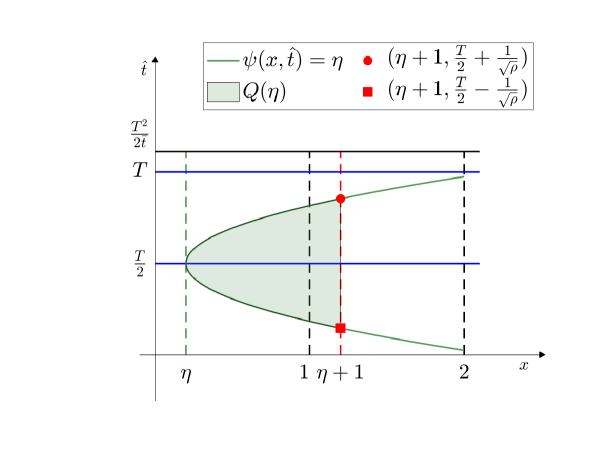
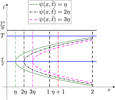
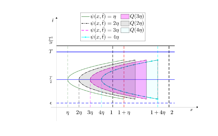
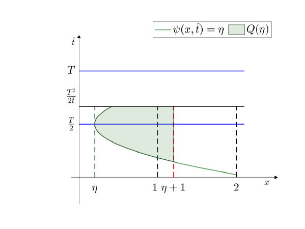
Figure 3: The sets , and .
In the sequel, we will denote by (resp. ) a generic positive constant independent of and (resp. independent of ).
Of course, both constants can change from line to line.
Taking into account the definition of (see Figure 3), we have from (16) that
(17)
for any and any .
Now, in view of (15), using the fact that in and in ,
we obtain from (17) that
and, therefore,
From the definition of and assmption (4), one has:
Thus, if we fix , we take and then rename as , we deduce that
(18)
Now, in order to get the best estimate, we minimize this quantity by choosing
and we deduce that
Then, using the classical Sobolev embedding and an interpolation inequality, for any , we obtain
whenever .
In particular, after a choice of in , one has for some independent of that
After integration with respect to and a variable change , we obtain:
Thus, using again interpolation, we see that, for any ,
where .
We note that can be taken arbitrarily close to and is independent of .
It is clear that .
Therefore, if , we have (12), which gives (9).
Case 2: .
Let us introduce again the function , given by (13).
In this case, we consider the sets
It is straightforward to see that the arguments applied in the previous case yield again (12).
Consequently, we also have (9) in this case.
Step 3: Let us establish the following lateral estimate of :
for every , there exist constants and such that
(20)
To this purpose, we first use Theorem 5.1 in [10] and deduce that
(21)
where and .
Then, we use an interpolation inequality
(22)
and we observe that (21) and (22) imply (20) when .
Finally, part b) of the lemma is straightforward:
it suffices to use (5) with , and arbitrarily small.
Remark 2.2
A similar result can be obtained when the right-hand side of the first equation in (3), is not zero.
Thus, if
and (for instance) , we can prove that, for any ,
(23)
for some and some .
Remark 2.3
A more involved argument is needed to take in (5) and (23).
The stability rate is expected to be weaker than single logarithmic.
This will be analyzed in a forthcoming paper.
3 Lateral estimates and uniqueness
This section is devoted to study the stability and uniqueness of (1) on the left part of the domain, .
Later, we will extend these results to and will obtain similar results in the whole domain .
Assume that
(24)
for .
Let us formulate an inverse problem concerning the left part of the domain:
Lateral uniqueness in :
Let , be two solutions to (24) in .
Assume that the corresponding observations coincide at the boundary , that is,
Then, do we have in and in with ?
As before, we will denote in the sequel by a generic positive constant.
We will also use , , , etc. to denote constants that can depend on .
The following proposition may be viewed as a first conditional stability result:
Proposition 3.1(Local stability for the lateral inverse problem)
Let us assume that
for some .
Also, let us assume that and
Then there exist , and such that
(25)
Proof:
For instance, let us assume that for and set .
Then, for all one has
Here, we have applied Lemma 2.1 to in combination with
the Mean Value Theorem to .
It is clear that we can get a similar estimate in the whole interval :
In addition to the assumptions in Corollary 3.3, let us assume that for some .
Then,
Corollary 3.5
In addition to the assumptions in Proposition 3.1, let us assume that for some with .
Then, for any small there exist and such that
(28)
Remark 3.6
If we do not assume that for some , then we do not have uniqueness in general.
Indeed, the following particular functions furnish a counter-example:
•
Let us set
where with and and .
Then satisfies the heat equation for and we observe that .
•
Let us take
and set for .
Then the functions and satisfy the Burgers’ equation respectively
in and and do not coincide (see for example [1, Section 2.1.2]).
However the associated and coincide.
4 Global estimates and uniqueness
In this section we will present global stability and uniqueness results for the inverse problem formulated in Section 1 in the whole domain .
Theorem 4.1(Conditional stability)
Let and be the solutions to (1) respectively corresponding
to the data , , , , , and and set and for
and all .
Assume that there exist constants and such that for all ,
Then, for every , there exist constants and such that
(29)
for all .
Proof:
We will find estimates of
in terms of , and and then we will use (25) and (26).
Let us set , for .
We introduce a change of variables to move from to .
For example, we set
Let the assumptions in Theorem 4.1 be satisfied and let us assume that in .
Then
(32)
Proof:
Given an arbitrary , we take .
For every , using Theorem 4.1 we can write that
Taking now , we see that
Finally, when , we see that
and, since , we deduce that in .
Acknowledgements
The first author was supported by the Grant PID2021-126813NB-I00 funded
by MCIN/AEI/10.1303
9/501100011033 and by “ERDF A way of making Europe” and
by the grant IT1615-22 funded the Basque Government.
The second and third authors were partially supported by MICINN, under Grant PID2020-114976GB-I00.
The fourth author was supported by Grant-in-Aid for Scientific Research (A) 20H00117 and Grant-in-Aid for Challenging Research (Pioneering) 21K18142 of the Japan Society for the Promotion of Science.
References
[1] J. Apraiz, A. Doubova, E. Fernández-Cara, M. Yamamoto, Some inverse problems for the Burgers equation and related systems, Communications in Nonlinear Science and Numerical Simulation 107 (2022), 106113.s
[2]
A.L. Bukhgeim and M.V. Klibanov, Global uniqueness of a class of
multidimensional inverse problems, Soviet. Math. Doklady 24, (1981), 244–247.
[3]
A. Doubova and E. Fernández-Cara, Some control results for simplified one-dimensional models of fluid-solid interaction, Mathematical Models & Methods in Applied Sciences 15, no. 5 (2005), 783–824.
[5]
M.V. Klibanov and A.A. Timonov, Carleman estimates for coefficient inverse
problems and numerical applications, Inverse and Ill-posed Problems Series, VSP, Utrecht, 2004.
[6]
Y. Liu, T. Takahashi, and M. Tucsnak, Single input controllability of a simplified fluid-structure interaction model, ESAIM: Control, Optimisation and Calculus of Variations 19 (2013) 20–42.
[7]
A. Munnier and E. Zuazua, Large time behavior for a simplified n-dimensional model of fluid–solid interaction, Communications in Partial Differential Equations 30, no. 3, (2005) 377–417.
[8] J.L. Vázquez and E. Zuazua, Lack of collision in a simplified 1-d model for fuid-solid interaction, Mathematical Models & Methods in Applied Sciences 16, no. 5, (2006), 637–678.
[9] J.L. Vázquez and E. Zuazua, Large time behavior for a simplified 1D model of fluid-solid interaction, Comm. Partial Differential Equations 28 (2003), no. 9–10, 1705–1738.
[10] M. Yamamoto, Carleman estimates for parabolic equations and applications, Inverse Problems 25 (2009) 123013.