Robust Performance Evaluation of
Independent and Identical Agents

Abstract

A principal provides nondiscriminatory incentives for independent and identical agents. The principal cannot observe the agents’ actions, nor does she know the entire set of actions available to them. It is shown, very generally, that any worst-case optimal contract is nonaffine in performances. In addition, each agent’s pay must depend on the performance of another. In the case of two agents and binary output, existence of a worst-case optimal contract is established and it is proven that any such contract exhibits joint performance evaluation — each agent’s pay is strictly increasing in the performance of the other. The analysis identifies a fundamentally new channel leading to the optimality of nonlinear team-based incentive pay.

“The incentive compensation scheme that is “correct” in one situation will not in general be correct in another. In principle, there could be a different incentive structure for each set of environmental variables. Such a contract would obviously be prohibitively expensive to set up; but more to the point, many of the relevant environmental variables are not costlessly observable to all parties to the contract. Thus, a single incentive structure must do in a variety of circumstances. The lack of flexibility of the piece rate system is widely viewed to be its critical shortcoming: the process of adapting the piece rate is costly and contentious.”
— NalebuffStiglitz_1983

1 Introduction

In the canonical moral hazard in teams model, a principal chooses a contract to incentivize a group of agents. Individual actions are unobservable, but stochastically affect observable individual performance. The optimal (Bayesian) contract thus exploits the statistical relationship between actions and performance indicators.

The canonical model has generated numerous economic insights relevant for policy analysis and management practice (holmstrom2017pay). However, it also has some well-known drawbacks. First, in practice, a few common forms of contracts, such as linear contracts and nonlinear bonus contracts, are used in a wide range of scenarios in which there is no compelling reason for there to be a common statistical justification. Second, managers may not possess well-defined prior beliefs over their agents’ production environment, limiting the applicability of the model’s practical guidance.

In response to these issues, an emerging literature in contract theory takes a non-Bayesian approach to the moral hazard in teams problem. In this literature, it is assumed that, while the principal may know about some actions her agents can take, she is uncertain about other actions that might be available to them. Hence, she chooses a contract that yields her maximal worst-case expected profits when considering all possible unknown actions available to the agents. A general finding is that contracts that are linear in performance indicators provide the best possible profit guarantees (see, for instance, Carroll_2015, DaiToikka_2018, and WaltonCaroll_2022).

One response to this striking and influential result is that the set of environments the principal considers is too “large” relative to the Bayesian literature. In practice, a manager may desire her contract to be robust, but also rule out certain production technologies as implausible. For instance, she may know her agents are independent and identical, but still want her contract to be robust to all possible technologies the agents may exploit within this class. The independent and identical agents setting is of particular interest not only because it is a benchmark setting in the Bayesian literature, but because existing arguments for linear contracts in the robust contracting literature rely on the ability of an agent to directly influence the performance of others.

Are robust contracts linear if a principal knows her agents are independent and identical? Do they link one agent’s pay to the performance of another? This paper shows, very generally, that any nondiscriminatory, worst-case optimal contract is nonaffine (and hence, nonlinear) and each agent’s pay depends on the performance of another. In the case of two agents and binary output, existence of a worst-case optimal contract is established and it is proven that any such contract exhibits joint performance evaluation, i.e., one agent’s pay increases in the performance of the other. This result provides novel foundations for nonlinear team-based incentive pay in the context of numerous existing results in the literature and identifies a channel leading to joint performance evaluation of potential relevance in practice.

A simple example illustrates the framework and key economic intuition.

Example 1. There is a risk-neutral residual claimant (manager) and two identical, risk-neutral agents that perform independent tasks. That is, it is common knowledge that their successes or failures are statistically independent, conditional on the actions they take, and that they cannot influence each other’s productivity. Successful completion of a task yields the manager a profit of one and failure yields her a profit of zero.

The manager knows that each agent can take one of two actions, “work” or “shirk”. She knows that “work” results in successful task completion with probability $p_{0}>0$ at effort cost $c_{0}\in(0,p_{0})$. On the other hand, she is uncertain about the effort cost of shirking, $c^{*}\in\mathbb{R}_{+}$, and the productivity of shirking, i.e., the probability $p^{*}<p_{0}$ with which it results in successful task completion.

The manager contemplates using one of two contracts, each of which is nondiscriminatory and respects agent limited liability:

1. Independent Performance Evaluation (IPE):
   Pay each agent $w\in(c_{0},1)$ for individual success and $0$ for failure.

2. Nonaffine Joint Performance Evaluation (JPE):
   Pay each agent a wage $w_{0}\in[0,w)$ for individual success and a team bonus

   $$b=\frac{w-w_{0}}{p_{0}}$$

   for joint success. Pay each agent $0$ for failure. Any such contract is calibrated to the contract-action pair $(w,\text{work})$ in the following sense: If an agent succeeds at her task, then her expected wage payment remains $w$ conditional on the other agent working. That is,

   $$w_{0}+bp_{0}=w.$$

The manager evaluates any contract according to the same criterion. First, for each value of $p^{*}$, she computes her expected payoff in her preferred Nash equilibrium in the game induced by the contract she offers. Second, she computes the infimum value of her expected payoff over all values of $c^{*}$ and $p^{*}$. The resulting payoff is called her worst-case payoff.

&   work         shirk
	work	$p_{0}w-c_{0}$ , $p_{0}w-c_{0}$	$p_{0}w-c_{0}$ , $p^{*}w-c^{*}$
	shirk	$p^{*}w-c^{*}$ , $p_{0}w-c_{0}$	$p^{*}w-c^{*}$ , $p^{*}w-c^{*}$

Figure 1: Game induced by IPE $w$ given $p^{*}$.

Can JPE yield the manager a higher worst-case payoff than IPE? The IPE contract $w$, together with an actual value of $p^{*}$, induces the game between the agents depicted in Figure 1. A naïve intuition is that the worst-case scenario for the principal occurs when $p^{*}=0$; if agents take a shirking action with this success probability, then the principal obtains an expected payoff of zero. But, this logic ignores incentives, as pointed out by Carroll_2015. In particular, each agent has a strict incentive to shirk if and only if she obtains a higher expected utility from doing so. Hence, $(\text{work},\text{work})$ is a Nash equilibrium whenever

$$p^{*}w-c^{*}\leq p_{0}w-c_{0}\iff p^{*}\leq p_{0}-\frac{(c_{0}-c^{*})}{w},$$

yielding the principal a payoff per agent of

$$p_{0}(1-w).$$

The principal’s worst-case payoff is instead obtained when $c^{*}=0$ and as $p^{*}$ approaches $p_{0}-\frac{c_{0}}{w}$ from above. Along this sequence, $(\text{shirk},\text{shirk})$ is the unique Nash equilibrium and the principal’s payoff per agent becomes arbitrarily close to

$$V_{IPE}(w)=(p_{0}-\frac{c_{0}}{w})(1-w).$$

Pay each agent $w\geq 0$ for individual success. Pay each agent $0$ for failure.

Joint Performance Evaluation (JPE): Pay each agent a wage $w_{0}\geq 0$ for individual success and a team bonus $b>0$ for joint success. Pay each agent $0$ for failure.

I prove the following result.

Theorem 3

1. If $\mu$ is sufficiently small and $p^{*}$ is sufficiently close to $p_{0}$, then the optimal IPE yields the principal strictly higher expected profits than any JPE.

2. If $\mu$ is sufficiently large, then there exists a JPE that yields the principal strictly higher expected profits than the optimal IPE.

Proof.

I make some preliminary observations about the optimal IPE. Observe that the optimal IPE that implements $a_{\emptyset}$ when the action set is $\{a_{\emptyset},a_{0}\}$ and $a^{*}$ when the action set is $\{a^{*},a_{\emptyset},a_{0}\}$ is the zero contract. The principal obtains an expected payoff per agent of

$$(1-\mu)p^{*}.$$

The optimal IPE implementing $a_{0}$ when the action set is $\{a_{\emptyset},a_{0}\}$ and $a^{*}$ when the action set is $\{a^{*},a_{\emptyset},a_{0}\}$ is

$$w^{*}=\frac{c_{0}}{p_{0}}.$$

The principal obtains an expected payoff per agent of

$$(\mu p_{0}+(1-\mu)p^{*})(1-\frac{c_{0}}{p_{0}}).$$

Finally, the optimal IPE always implementing $a_{0}$ is

$$\hat{w}=\frac{c_{0}}{p_{0}-p^{*}}.$$

The principal obtains an expected payoff per agent of

$$p_{0}(1-\frac{c_{0}}{p_{0}-p^{*}}).$$

Any other implementation is either infeasible or suboptimal. I now separately consider the cases in which $\mu$ is small and $\mu$ is large to establish the results.

1. If $\mu$ is sufficiently small and $p^{*}$ is sufficiently close to $p_{0}$, then

   $$(1-\mu)p^{*}>\max\{\left(\mu p_{0}+(1-\mu)p^{*}\right)(1-\frac{c_{0}}{p_{0}}),p_{0}(1-\frac{c_{0}}{p_{0}-p^{*}})\}.$$

   Hence, the optimal IPE puts $w^{*}=0$, yielding the principal a per-agent payoff of

   $$(1-\mu)p^{*}.$$

   On the other hand, for a given JPE, $(w_{0},b)$, the principal obtains a per-agent payoff no larger than

   $$(1-\mu)(p^{*}(1-(w_{0}+p^{*}b))),$$

   when $\mu$ is sufficiently small. Because $p^{*}b>0$, this means the principal can do no better than the optimal IPE.

2. If $\mu$ is sufficiently large, then

   $$\left(\mu p_{0}+(1-\mu)p^{*}\right)(1-\frac{c_{0}}{p_{0}})>\max\{p_{0}(1-\frac{c_{0}}{p_{0}-p^{*}}),(1-\mu)p^{*}\}.$$

   Hence, in these cases, $w^{*}=\frac{c_{0}}{p_{0}}$ is the optimal IPE. Now, consider a calibrated JPE with $w_{0}\in(0,w^{*})$ and $b=\frac{w^{*}-w_{0}}{p_{0}}>0$. The principal’s per-agent payoff from this contract is

   $$\mu\left(p_{0}(1-w^{*})\right)+(1-\mu)\left(p^{*}(1-(w_{0}+p^{*}b))\right)>$$

   $$\mu\left(p_{0}(1-w^{*})\right)+(1-\mu)\left(p^{*}(1-(w_{0}+p_{0}b))\right)=\underbrace{(\mu p_{0}+(1-\mu)p^{*})(1-\frac{c_{0}}{p_{0}})}_{\text{Payoff $w^{*}$}}.$$

   Hence, the constructed JPE strictly outperforms the optimal IPE.

∎

B.3 Discriminatory Contracts

An asymmetric (discriminatory) contract is a quadruple $w^{i}=(w^{i}_{11},w^{i}_{10},w^{i}_{01},w^{i}_{00})\in\mathbb{R}^{4}_{+}$ for each agent $i=1,2$, where the first index of each wage indicates agent $i$’s success or failure and the second indicates agent $j$’s success or failure. It is an independent performance evaluation (IPE) if $w^{i}_{y1}=w^{i}_{y0}$ for each agent $i=1,2$ and success or failure $y\in\{0,1\}$.

Recall that the analysis of the optimal symmetric contract yields

$$V(w^{*}):=\underset{w_{11}>w_{10}\geq 0}{\max}\leavevmode\nobreak\ \leavevmode\nobreak\ \min\{1-w_{11},\bar{p}\left[\bar{p}(1-w_{11})+(1-\bar{p})(1-w_{10})\right]\},$$

where $\bar{p}$ is the solution to the initial value problem in the statement of Lemma LABEL:JPE_worst. The worst-case payoff from a general IPE can be identified as the value of an appropriately defined max-min problem:

$$V^{**}_{IPE}:=\quad\underset{w_{1}\geq w_{2}\geq 0}{\max} \underset{a^{*}_{1},a^{*}_{2}}{\min}\quad\left[p(a^{*}_{1})(1-w_{1})+p(a^{*}_{2})(1-w_{2})\right]$$

subject to

$$p(a^{*}_{1})w_{1}-c(a^{*}_{1})\geq\underset{a_{0}\in A^{0}\cup\{a^{*}_{1},a^{*}_{2}\}}{\max}\left[p(a_{0})w_{1}-c(a_{0})\right]$$

$$p(a^{*}_{2})w_{2}-c(a^{*}_{2})\geq\underset{a_{0}\in A^{0}\cup\{a^{*}_{1},a^{*}_{2}\}}{\max}\left[p(a_{0})w_{2}-c(a_{0})\right],$$

where $w_{1}$ is the wage agent 1 receives conditional upon individual success and $w_{2}$ is the corresponding wage for agent 2 (it is optimal to pay each agent zero for individual failure). The constraints in the minimization problem ensure that each agent $i$ has an incentive to take a worst-case unknown action $a^{*}_{i}$. No other constraints are required since one agent’s optimal action is unaffected by the chosen action of the other.

In the running example in which there is a single known action, $a_{0}$, with $p(a_{0})=1$ and $c(a_{0})=\frac{1}{4}$, the optimal wages are $w^{*}_{11}=\frac{2}{3}$ and $w^{*}_{10}=w^{*}_{01}=w^{*}_{00}=0$ yielding the principal a worst-case payoff of $V(w^{*})=\frac{1}{3}$. Figure 9 shows that, in this case, $V^{**}_{IPE}$ lies below $\frac{1}{3}$. Figure 10 shows, however, that if $c(a_{0})$ is increased to $\frac{3}{4}$, then there exist wages $w_{1}\neq w_{2}$ that yield the principal a strictly higher worst-case payoff than under the optimal JPE, i.e. $V^{**}_{IPE}>V(w^{*})$. The optimality of discrimination thus depends on the cost of effort of each agent in the principal’s target action profile.

Figure 9: The orange surface represents the principal’s worst-case payoff on the z-axis as discriminatory individual wages $w_{1}$ and $w_{2}$ vary. The blue surface plots the principal’s worst-case payoff under the optimal nondiscriminatory JPE. Parameters: $p(a_{0})=1$ and $c(a_{0})=\frac{1}{4}$.

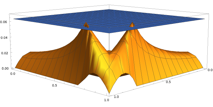
Figure 10: The orange surface represents the principal’s worst-case payoff on the z-axis as discriminatory individual wages $w_{1}$ and $w_{2}$ vary. The blue surface plots the principal’s worst-case payoff under the optimal nondiscriminatory JPE. Parameters: $p(a_{0})=1$ and $c(a_{0})=\frac{3}{4}$.

B.4 Asymmetric Unknown Actions

Let $\mathcal{E}(w,A_{1},A_{2})$ denote the set of Nash equilibria in the game induced by the contract $w$ and action sets $A_{1}$ and $A_{2}$. In addition, let

$$V(w):=\underset{a^{*}_{1},a^{*}_{2}\in\mathbb{R}_{+}\times[0,1]}{\min}\quad\underset{\sigma\in\mathcal{E}(w,\{a_{0},a^{*}_{1}\},\{a_{0},a^{*}_{2}\})}{\max}E_{\sigma}[y_{1}+y_{2}-w_{y_{1}y_{2}}-w_{y_{2}y_{1}}].$$

Then, the following result holds.

Theorem 4

Suppose there is a single known action $a_{0}$ with $p(a_{0})>c(a_{0})>0$ and each agent has at most one unknown action. Then, even if unknown actions can differ across agents, there exists a nonaffine JPE, $w$, for which $V(w)>V^{*}_{IPE}$.

Proof.

Suppose $w$ is a nonlinear JPE with $w_{00}=w_{01}=0$. Then, $V(w)$ is the minimum of

$$2-2w_{11},$$

the principal’s payoff when both agents succeed with probability one, and

$$p_{1}p_{2}(2-2w_{11})+(p_{1}(1-p_{2})+p_{2}(1-p_{1}))(1-w_{10}),$$

where

$$p_{1}:=p(a_{0})-\frac{c(a_{0})}{(p(a_{0})w_{11}+(1-p(a_{0}))w_{10})}$$

and

$$p_{2}:=p(a_{0})-\frac{c(a_{0})}{(p_{1}w_{11}+(1-p_{1})w_{10})}.$$

The second expression corresponds to the principal’s payoff in the limit of a sequence of games in which iterated elimination of strictly dominated strategies first removes $a_{0}$ for worker 1 and, second, removes $a_{0}$ for worker 2, leading to a unique Nash equilibrium in which worker 2 is even less productive than in the symmetric worst-case limit.

I establish the existence of a calibrated JPE, $w$, for which $V(w)>V^{*}_{IPE}$. Let $w^{*}=\sqrt{c(a_{0})/p(a_{0})}$ be the optimal IPE. Put $w_{10}=w^{*}-\epsilon$, for $\epsilon>0$, and

$$w_{11}=\frac{w^{*}-(1-p(a_{0}))w_{10}}{p(a_{0})}.$$

It suffices to show that the right-derivative of profits with respect to $\epsilon$ evaluated at zero is strictly positive to establish the existence of a nonlinear JPE that outperforms the best IPE. For $\epsilon>0$, the derivative of profits is well-defined and equals

$$p(a_{0})w^{*}-\frac{c(a_{0})}{(1-\epsilon)^{2}}.$$

Hence, the right-derivative evaluated at zero is strictly positive whenever

$$p(a_{0})w^{*}-c(a_{0})>0\iff p(a_{0})>c(a_{0}),$$

which always holds. ∎

B.5 Pessimistic Equilibrium Selection

Denote the set of (weakly) Pareto Efficient Nash equilibria by $\mathcal{E}_{P}(w,A)$. In contrast to the model analyzed in the main text, let the principal’s expected payoff given a contract $w$ and action set $A\supseteq A^{0}$ be given by

$$V(w,A):=\underset{\sigma\in\mathcal{E}_{P}(w,A)}{\min}E_{\sigma}[y_{1}+y_{2}-w_{y_{1}y_{2}}-w_{y_{2}y_{1}}].$$

Notice that the principal assumes the agents will play her least-preferred equilibrium. As before, the principal’s worst case payoff from a contract $w$ is

$$V(w):=\underset{A\supseteq A^{0}}{\inf}\leavevmode\nobreak\ V(w,A).$$

In analyzing the nature of the solution to the principal’s problem, I will need one additional definition. If $\Gamma(w,A)$ is a supermodular game and $U_{i}(a_{i},a_{j};w)$ is strictly increasing in $p(a_{j})$ when $p(a_{i})>0$, then $\Gamma(w,A)$ is said to exhibit strictly positive spillovers. The following result has been previously established in the literature.

Lemma 11 (Vives_1990, MilgromRoberts1990)

Suppose $\bar{a}$ ($\underline{a}$) is the limit found by iterating $\overline{BR}$ ($\underline{BR}$) starting from $a_{\max}$ ($a_{\min}$). If $\Gamma(w,A)$ is supermodular, then it has a maximal Nash equilibrium $(\bar{a},\bar{a})$ and a minimal Nash equilibrium $(\underline{a},\underline{a})$; any other equilibrium $(a_{i},a_{j})$ must satisfy $\bar{a}\succeq a_{i}\succeq\underline{a}$ and $\bar{a}\succeq a_{j}\succeq\underline{a}$. If, in addition, $\Gamma(w,A)$ exhibits strictly positive spillovers, then $(\bar{a},\bar{a})$ is the unique Pareto Efficient Nash equilibrium.

Notice that, if $w$ is a JPE for which $w_{00}=w_{01}=0$ and $A\supseteq A^{0}$, then $\Gamma(w,A)$ is a supermodular game exhibiting strictly positive spillovers. Hence, the principal assumes agents will play the maximal equilibrium in any game the agents play. I use this observation to establish the following result.

Theorem 5

Under pessimistic equilibrium selection, any worst-case optimal contract must be nonlinear and cannot be an IPE.

Proof.

I first show that, for any linear contract $w$, $V(w)<V^{*}_{IPE}$. I first argue that any eligible linear contract must have $0<\alpha<1$. Towards contradiction, suppose $\alpha=0$. Then, the assumption of costly known actions ensures that $w$ cannot guarantee the principal more than zero in the game $\Gamma(w,A^{0}\cup\{a_{\emptyset}\})$, where $p(a_{\emptyset})=c(a_{\emptyset})=0$. (In this game, each agent has a strict incentive to choose $a_{\emptyset}$ yielding the principal a payoff of zero.) If $\alpha\geq 1$, then the assumption of costly known actions ensures that $w$ cannot guarantee the principal more than zero in the game $\Gamma(w,A^{0}\cup\{a_{\delta_{1}}\})$, where $p(a_{\delta_{1}})=1$ and $c(a_{\delta_{1}})=0$. (In this game, each agent has a strict incentive to choose $a_{\delta_{1}}$, yielding the principal a payoff of $2-2\alpha\leq 0$.)

Let $\alpha\in(0,1)$ parameterize the eligible linear contract $w$. Let $a_{0}\in A^{0}$ be each agent’s maximal equilibrium action when $A=A^{0}$ (since any linear contract is a JPE, such an action exists by Lemma 11). In the game $\Gamma(w^{\prime},A^{0}\cup\{a^{*}_{\epsilon}\})$, where $p(a^{*}_{\epsilon})=p(a_{0})-\frac{c(a_{0})}{\alpha}+\epsilon$, $c(a^{*}_{\epsilon})=0$, and $\epsilon>0$ is small, $(a^{*},a^{*})$ is the maximal Nash equilibrium. As $\epsilon$ approaches $0$, the principal’s payoff in this equilibrium approaches

$$2\left[\underbrace{\left(p(a_{0})-\frac{c(a_{0})}{\alpha}\right)}_{\text{$>0$ by eligibility of $w$}}\left(\left(p(a_{0})-\frac{c(a_{0})}{\alpha}\right)(1-\alpha)+(1-\left(p(a_{0})-\frac{c(a_{0})}{\alpha}\right))(-\alpha)\right)\right]$$

$$<2\left[\left(p(a_{0})-\frac{c(a_{0})}{\alpha}\right)\left(1-\alpha\right)\right]$$

$$\leq V^{*}_{IPE}.$$

Hence,

$$V(w)\leq\quad\underset{\epsilon>0}{\inf}\quad V(w,A^{0}\cup\{a^{*}_{\epsilon}\})<V^{*}_{IPE}.$$

Now, observe that the proof of Lemma LABEL:JPE_worst in Section LABEL:JPEworst_proof holds as written under worst-case Pareto Efficient Nash equilibrium selection. Hence, there exists a JPE $w$ with $w_{00}=w_{01}=0$ for which $V(w)>V^{*}_{IPE}$. It follows that no worst-case optimal contract can be an IPE. ∎

I remark that the result and proof extend to the case in which there are $n\geq 2$ agents and the set of output levels is a compact set, $Y$, with $\min(Y)=0<\max(Y)$.