Hydrodynamic limit for a boundary-driven Facilitated Exclusion Process

Abstract.

We study the symmetric facilitated exclusion process (FEP) on the finite one-dimensional lattice $\{1,\ldots,N-1\}$ when put in contact with boundary reservoirs, whose action is subject to an additional kinetic constraint in order to enforce ergodicity. We study in details its stationary states in various settings, and use them in order to derive its hydrodynamic limit as $N\to\infty$, in the diffusive space-time scaling, when the initial density profile is supercritical. More precisely, the macroscopic density of particles evolves in the bulk according to a fast diffusion equation as in the periodic case, and besides, we show that the boundary-driven FEP exhibits a very peculiar behaviour: unlike for the classical SSEP, and due to the two-phased nature of the FEP, the reservoirs impose Dirichlet boundary conditions which do not coincide with their equilibrium densities. The proof is based on the classical entropy method, but requires significant adaptations to account for the FEP’s non-product stationary states and to deal with the non-equilibrium setting.

1. Introduction

Over the last century, there has been a rapidly growing interest in describing macroscopic features of the physical world at the microscopic level. In particular, a variety of models has been introduced to describe the evolution of a multiphased media, as for instance the joint evolution of liquid and solid phases. Such complex phenomena often feature absorbing phase transitions, which have been closely investigated by both physicists and mathematicians over the last decades.

In particular, the class of kinetically constrained stochastic lattice gases, which has been put forward in the 80’s (see e.g. [RS03] for a review), is known to accurately illustrate some microscopic mechanisms at the origin of liquid/solid interfaces. In these systems, particles are situated on the sites of a discrete lattice, and jump at random times to neighbouring sites, following microscopic rules: we consider here in particular the exclusion rule, which prevents two particles from being on the same site, and an additional kinetic constraint, which makes the jump possible or not depending locally on the configuration around. Such kinetically constrained lattice gases can be seen as the Kawasaki-type counterparts to the Glauber-type non-conservative kinetically constrained spin models (see e.g. [TB07] and [CMRT09] for a more exhaustive review), whose dynamics involves particle creation/annihilation rather than jumps.

One of these models, called facilitated exclusion process (FEP) has been proposed by physicists in [RPSV00] and further investigated by physicists and mathematicians in, for instance, [Lub01, dO05, BM09, BBCS16, BESS20, BES21]. The one-dimensional FEP on the discrete lattice $\Lambda\subset\mathbb{Z}$ is defined as follows: it is an exclusion process, meaning that each site is either empty or occupied by one particle. Besides, a particle is considered active if at least one of its two neighbouring sites is occupied. Then, active particles jump randomly at rate 1 to any empty nearest neighbour. Because of the kinetic constraint, the FEP exhibits phase separation with critical density $\rho_{c}=\frac{1}{2}$: it remains active at supercritical densities $\rho>\frac{1}{2}$ whereas it quickly reaches an absorbing state, i.e. a particle configuration with no active particle, if $\rho<\frac{1}{2}$. The FEP is cooperative, in the sense that there is no mobile cluster of particles in the system. The cooperative nature of the FEP distorts its equilibrium measures, which are no longer product, thus generating significant difficulties. Nevertheless, in the supercritical regime, the grand-canonical states $\pi_{\rho}$ are explicit, and supported by the ergodic component, namely the set of configurations where empty sites are all surrounded by particles. Those grand-canonical states $\pi_{\rho}$ are translation invariant and can be defined sequentially, through a Markovian construction, by filling an arbitrary site with probability $\rho>\frac{1}{2}$, and following each particle by another particle with probability $\mathfrak{a}(\rho)=(2\rho-1)/\rho$. This quantity $\mathfrak{a}(\rho)$ represents the density of active particles in the system at density $\rho$. To make sure empty sites are isolated, each empty site is instead followed by a particle with probability $1$.

In [BESS20, BES21], the hydrodynamic limit of the symmetric FEP with periodic boundary conditions is derived, and takes the form of a Stefan (or free boundary) problem with (non-linear) diffusion coefficient $D(\rho)=\mathfrak{a}^{\prime}(\rho)\mathds{1}\{\rho>\frac{1}{2}\}$. In other words, the diffusive supercritical phase (i.e. the macroscopic regions where $\rho_{0}(u)>\frac{1}{2}$) progressively invades the frozen subcritical phase (where $\rho_{0}(u)<\frac{1}{2}$), until one of the phases disappears (depending on the total mass $\int\rho_{0}$ of the initial density profile being super- or sub-critical). For asymmetric jump rates, the hyperbolic Stefan problem hydrodynamic limit was derived in [ESZ22]. More recently, the stationary macroscopic equilibrium fluctuations have been characterized in the symmetric, weakly asymmetric and asymmetric cases in [EZ23]. All these results rely in parts on mapping arguments which fail in dimension higher than $1$. The stationary and absorbing states for the FEP were also extensively studied both in the symmetric and asymmetric cases [GLS19, GLS21, GLS22, CZ19], and once again rely on mapping arguments.

As the effect of boundary interactions on lattice gases has been under considerable scrutiny in recent years, it is now natural to investigate the macroscopic effect of boundary dynamics on the FEP. Adding reservoir-type interactions at the extremities of microscopic systems is a classical way to induce boundary conditions at the macroscopic level (e.g. in the hydrodynamic PDE), see for instance [Gon19] for a recent review in the case of symmetric simple exclusion (SSEP). In turn, these boundary effects give access to the macroscopic non-equilibrium features of the model considered [Der07, Der11]. In the FEP, particles injected by reservoirs may become blocked by the kinetic constraint, and therefore change the effective stationary density imposed by the reservoirs, so that the effect of reservoir dynamics on the FEP is far from trivial.

In this work, we consider the boundary-driven one-dimensional symmetric FEP on the finite lattice $\Lambda_{N}:=\{1,\dots,N-1\}$, with two stochastic reservoirs at the extremities, whose dynamics is illustrated in Figure 1. To avoid degenerate behaviour, particles in contact with the reservoirs are always active, meaning that if a particle is situated at one of the two extremities $x=1$ or $x=N-1$, then it can always jump towards the bulk. Stochastic reservoirs at both ends inject particles at the extremities, if they are empty, at rate $\alpha,\;\beta\in(0,1)$. They can also remove a boundary particle, at rate $1-\alpha$, $1-\beta$, provided that the boundary particle is followed by another particle. This new kinetic constraint imposed at both reservoirs is not standard. It is made with the main purpose of preserving ergodic configurations: namely, if the particle system starts from an ergodic state $\eta(0)$ (where every empty site is surrounded by particles), then it is not difficult to see that at any time $t>0$, $\eta(t)$ remains ergodic. With another definition of the reservoirs, the ergodic component would not remain stable under the dynamics, and this would raise considerable difficulties from a hydrodynamic limit standpoint.

Remarkably, a simple argument shows that unconstrained reservoirs with density $\alpha$, i.e. the classical ones which remove particles at rate $1-\alpha$ without requiring another neighbouring particle, create unusual boundary conditions at the level of the macroscopic density: they impose at the boundary an active density $\mathfrak{a}(\rho)$ equal to $\alpha$, rather than a density $\rho$ equal to $\alpha$, as it is already well-known for the SSEP, for example. However, this framework raises significant technical difficulties, in particular very few information is available on the stationary states, thus it is left for future work.

Figure 1. Illustration of the dynamics in the bulk (above) and on the left boundary (below). Allowed jumps are denoted by $\checkmark$. Forbidden jumps are denoted by $\times$.

To focus on the most salient challenges of boundary interactions, we start our process straight from the ergodic component, in order to avoid some issues related to transience time for the FEP. Therefore, the microscopic system is assumed to be initially already one-phased, with a uniformly-supercritical density. Thus, we consider here the boundary-driven symmetric FEP in the diffusive time-scale, started from an ergodic initial configuration fitting a supercritical density profile $\rho^{\rm ini}:[0,1]\to(\frac{1}{2},1]$. Our main result states that its hydrodynamic limit $\rho(t,u)$ is the unique (very weak) solution to

$$\partial_{t}\rho=\partial_{u}^{2}\mathfrak{a}(\rho),\qquad\rho(0,\cdot)=\rho^{\rm ini}$$ (1)

with Dirichlet boundary conditions

$$\rho(\cdot,0)\equiv\overline{\rho}(\alpha),\qquad\rho(\cdot,1)\equiv\overline{\rho}(\beta),$$

for some explicit function $\alpha\longmapsto\overline{\rho}(\alpha)>\frac{1}{2}$, representing the effective density imposed on the FEP by a reservoir with density $\alpha$. The general case where the initial profile takes any values in $[0,1]$ is technically challenging, partly because mappings are not available in the presence of reservoirs since the total number of particles is no longer conserved. We fully expect, however, that the hydrodynamic limit holds in that case as well and takes the form of a Stefan problem as in the periodic case. This is also left for future work.

Let us now present briefly the strategy of the proof and its main novelties. As the hydrodynamic limit plays the role of a law of large numbers for the empirical density of particles, the detailed knowledge of the stationary states is a crucial element in the proof. As expected, this is particularly challenging for the FEP (whose equilibrium states are not product [BESS20]), and even more so in the non-equilibrium setting $\alpha\neq\beta$, which induces long-range correlations. For that reason, we start by building explicitly the one-reservoir, semi-infinite stationary state using a refined Markov construction inspired by previous work [EZ23]. We also explicitly derive the equilibrium stationary state in the presence of two reservoirs with $\alpha=\beta$, for which no Markovian construction is available, but which is uniform over ergodic configurations with a fixed number of particles. Finally, we construct an approximation of the stationary state in the non-equilibrium case $\alpha\neq\beta$, inspired by the previous ones, using the fact that the active density in the bulk should interpolate linearly between its two boundary values. This construction is not trivial, and needs to be supplemented by quantitative density and correlation estimates to derive the hydrodynamic limit. The rest of the proof then follows the entropy method, relying on the classical one-block and two-blocks estimates. However, even more so than in the periodic case, some care is required to handle the fact that the approximated stationary states are not product, thus do not lend themselves easily to conditioning to local boxes.

This article is organized as follows. In Section 2, we introduce the FEP in contact with constrained reservoirs starting from the ergodic component, and state our main result, Theorem 2.4, namely the hydrodynamic limit for the boundary-driven FEP. In Section 3, we study in great details its local stationary states. Section 4 is dedicated to building an approximate stationary state for the non-equilibrium FEP, inspired by the explicit results obtain in the previous section. Once the approximate stationary state is built, we obtain in the rest of Section 4 the associated density, correlation field and dynamical Dirichlet estimates. In Section 5, we finally exploit those Dirichlet estimates, in order to adapt the classical entropy method and complete the proof of the hydrodynamic limit. Since significant adaptations need to be made, we expose in detail the proof of the classical one and two-blocks estimates in Section 6.

2. Model and results

2.1. General notations

We gather here some general notations that will be used throughout this article.

• We let $\mathbb{N}=\{0,1,2,\ldots\}$ denote the set of non-negative integers, and $\mathbb{N}^{*}=\mathbb{N}\setminus\{0\}$. We use double brackets $\llbracket$ to denote integer segments, e.g. if $a,b\in\mathbb{N}$ are such that $a<b$, $\llbracket a,b\rrbracket=\{a,a+1,\dots,b-1,b\}$, and $\rrbracket a,b\llbracket=\{a+1,\dots,b-2,b-1\}$.

• The integer $N\in\mathbb{N}^{*}$ is a scaling parameter that shall go to infinity.

• Given two functions $f,g\in L^{2}\big{(}[0,1]\big{)}$, we denote by

  $$\langle f,g\rangle=\int_{0}^{1}f(u)g(u)\,\mathrm{d}u$$

  their $L^{2}$ scalar product. If $m$ is a finite measure on $[0,1]$ and $f\in L^{2}(m)$, we also denote by $\langle m,f\rangle$ the integral of $f$ with respect to $m$.

• For any non-negative sequence $(u_{k})_{k\in\mathbb{N}}$ possibly depending on other parameters than $k$, we will denote by $\mathcal{O}_{k}(u_{k})$ (resp. $o_{k}(u_{k})$) an arbitrary sequence $(v_{k})_{k\in\mathbb{N}}$ for which there exists a constant $C>0$ (resp. a vanishing sequence $(\varepsilon_{k})_{k\in\mathbb{N}}$) – possibly depending on other parameters – such that

  $$\forall k\in\mathbb{N},\qquad|v_{k}|\leqslant Cu_{k}\qquad(\mbox{resp. }|v_{k}|\leqslant\varepsilon_{k}u_{k}).$$

  In the absence of ambiguity in the parameters, we simply write $\mathcal{O}(u_{k})$ and $o(u_{k})$.

• A particle configuration is an element $\eta\in\{0,1\}^{\Lambda}$ for some $\Lambda\subset\mathbb{N}^{*}$. Given a function $g(\eta)$, and given a time trajectory $\eta(t),\;t\geqslant 0$, whenever convenient we will simply write $g(t)$ for $g(\eta(t)).$

• When a new notation is introduced inside of a paragraph and is going to be used throughout, we colour it in blue.

2.2. Definition of the model

Let us introduce the facilitated exclusion process with boundary dynamics which is investigated in this paper. This particle system is evolving on a finite one-dimensional lattice of size $N-1$, called its bulk ${\color[rgb]{.15,.0.35,.85}\Lambda_{N}=\llbracket 1,N-1\rrbracket}$. A particle configuration is a variable $\eta=(\eta_{x})_{x\in\Lambda_{N}}\in{\color[rgb]{.15,.0.35,.85}\Omega_{N}:=\{0,1\}^{\Lambda_{N}}}$, where, as usual for exclusion processes, $\eta_{x}=1$ (resp. $\eta_{x}=0$) means that site $x\in\Lambda_{N}$ is occupied by a particle (resp. empty). We consider here the symmetric Facilitated Exclusion Process (FEP), where particles jump at rate $1$ to each neighbouring site provided the target site is empty (exclusion rule) and that its other neighbouring site is occupied (kinetic constraint). In other words, the Markov generator $\mathcal{L}_{0}$ ruling the bulk dynamics for the FEP is defined as follows: for any $f:\Omega_{N}\to\mathbb{R}$, and any $\eta\in\Omega_{N}$,

$$\mathcal{L}_{0}f(\eta)=\sum_{x=1}^{N-2}c_{x,x+1}(\eta)\big{[}f(\eta^{x,x+1})-f(\eta)\big{]},$$ (2)

where

$$c_{x,x+1}(\eta)=\eta_{x-1}\eta_{x}\big{(}1-\eta_{x+1}\big{)}+\big{(}1-\eta_{x}\big{)}\eta_{x+1}\eta_{x+2},$$ (3)

is the jump rate encompassing both constraints, and

$$\forall z\in\Lambda_{N},\quad\eta^{x,y}_{z}=\begin{cases}\eta_{z}&\mbox{ if }z\neq x,y,\\ \eta_{y}&\mbox{ if }z=x,\\ \eta_{x}&\mbox{ if }z=y.\end{cases}$$ (4)

In other words, $\eta^{x,y}$ is the configuration where the values at sites $x$ and $y$ have been exchanged. Note that sites $0$ and $N$ do not belong to the bulk, so that when $x=1$ or $N-2$, in (3), we define by convention ${\color[rgb]{.15,.0.35,.85}\eta_{0}=\eta_{N}=1}$. Namely, a particle at one of the boundaries (i.e. $x=1$ or $x=N-1$) is always able to jump to the neighbouring site if it is empty, without being subject to any kinetic constraint.

Let us fix two parameters ${\color[rgb]{.15,.0.35,.85}\alpha,\;\beta\in(0,1)}.$ At both ends, we put the FEP in contact with stochastic reservoirs of particles with densities $\alpha$ and $\beta$, in the following way;

• if site $x=1$ (resp. $x=N-1$) is empty, then the left (resp. right) reservoir injects a particle at rate $\alpha$ (resp. $\beta$) at this site ;

• if there is a particle at site $x=1$ (resp. $x=N-1$), then the reservoir absorbs it at rate $1-\alpha$ (resp. $1-\beta$) only if site $x=2$ (resp. $x=N-2$) is also occupied. This additional constraint in case of absorption is consistent with the bulk kinetic constraint: in order to leave the system, a particle also needs an occupied neighbour.

The reservoir dynamics are therefore ruled by the following Markov generators: for any $f:\Omega_{N}\to\mathbb{R}$ and any $\eta\in\Omega_{N}$,

$$\mathcal{L}_{\ell}f(\eta)=b_{\ell}(\eta)\big{[}f(\eta^{1})-f(\eta)\big{]}\qquad\mbox{ and }\qquad\mathcal{L}_{r}f(\eta)=b_{r}(\eta)\big{[}f(\eta^{N-1})-f(\eta)\big{]}$$ (5)

with boundary rates given by

$$b_{\ell}(\eta)=\alpha\big{(}1-\eta_{1}\big{)}+(1-\alpha)\eta_{1}\eta_{2}\qquad\mbox{ and }\qquad b_{r}(\eta)=\beta\big{(}1-\eta_{N-1}\big{)}+(1-\beta)\eta_{N-1}\eta_{N-2}$$ (6)

and where $\eta^{x}$ is the configuration obtained from $\eta$ by flipping the coordinate $x$:

$$\eta^{x}_{z}=\begin{cases}\eta_{z}&\mbox{ if }z\neq x,\\ 1-\eta_{x}&\mbox{ if }z=x.\end{cases}$$ (7)

As already pointed out in [BESS20], the FEP belongs to the class of gradient models because the instantaneous density current in the bulk, namely $j_{x,x+1}(\eta)=c_{x,x+1}(\eta)\big{(}\eta_{x}-\eta_{x+1}\big{)}$, with $x\in\llbracket 1,N-2\rrbracket$, can be written under the form $j_{x,x+1}(\eta)=h_{x}(\eta)-h_{x+1}(\eta)$ where $h_{x}$ is the local function defined by

$$h_{x}(\eta)=\eta_{x-1}\eta_{x}+\eta_{x}\eta_{x+1}-\eta_{x-1}\eta_{x}\eta_{x+1}.$$ (8)

Here, the gradient decomposition is valid for any $x\in\llbracket 1,N-2\rrbracket$, and we note that, with our convention, $h_{1}(\eta)=\eta_{1}$ and $h_{N-1}(\eta)=\eta_{N-1}$. More importantly, this function can be interpreted as the indicator function that an active particle lies at site $x$, where active means that the particle has at least one occupied neighbour.

The boundary-driven symmetric FEP is therefore ruled by the total generator

$$\mathcal{L}_{N}:=\mathcal{L}_{0}+\mathcal{L}_{\ell}+\mathcal{L}_{r}.$$ (9)

Let us fix $T>0$. Given a probability measure $\mu$ on $\Omega_{N}$, we denote by ${\color[rgb]{.15,.0.35,.85}\mathbb{P}_{\mu}}$ the distribution on the Skorokhod space $\mathcal{D}([0,T],\Omega_{N})$ of the process $\{\eta(t),\;t\geqslant 0\}$ driven by the diffusively accelerated generator $N^{2}\mathcal{L}_{N}$, and with initial distribution $\mu$. We denote by ${\color[rgb]{.15,.0.35,.85}\mathbb{E}_{\mu}}$ the corresponding expectation. Note that, even though the process $\eta(t)$ strongly depends on $N$, via the time scale and the state space, this dependence does not appear in our notation, for the sake of clarity.

2.3. Frozen and ergodic configurations

In the absence of boundary interactions, the FEP exhibits a phase separated behaviour, which depends on the local particle density (see [BESS20, BES21] for a detailed study in the periodic case). More precisely, let us define its critical density ${\color[rgb]{.15,.0.35,.85}\rho_{c}:=\frac{1}{2}}$. If the process starts from a product state with subcritical density $\rho<\rho_{c}$, then, after a transience time (which has been estimated in [BESS20]), almost surely every particle has become isolated (surrounded by empty sites), i.e. the FEP has reached its frozen component ${\color[rgb]{.15,.0.35,.85}\mathcal{F}:=\{\eta:\eta_{x}\eta_{x+1}=0,\;\forall x\}}$, in which no particle is active. If instead, the process is started from a supercritical density (greater than $\rho_{c}$), then, after a transience time, it has reached its ergodic component ${\color[rgb]{.15,.0.35,.85}\mathcal{E}:=\{\eta:\eta_{x}+\eta_{x+1}\geqslant 1,\;\forall x\}}$, in which all empty sites are isolated (surrounded by occupied ones), in other words, all particles in $\mathcal{E}$ are active. In fact, it is easy to check that pairs of neighbouring empty sites can be separated by the dynamics, but not created. For this reason, once all empty sites are isolated, the configuration has reached an ergodic component which is irreducible for the Markov process. We give in Figure 2 an example (in our boundary-driven setting) of an ergodic configuration in $\Omega_{13}$ where we highlight its active particles (i.e. those which either have an occupied neighbour or are at the boundaries of the system).

Figure 2. An ergodic configuration and its active particles (in orange).

Throughout, given a set $B\subset\mathbb{Z}$, we define the ergodic component $\mathcal{E}_{B}$ as the set of configurations on $B$ where two neighbouring sites in $B$ contain at least one particle, namely

$$\mathcal{E}_{B}:=\Big{\{}\eta\in\{0,1\}^{B}:\eta_{x}+\eta_{x+1}\geqslant 1\mbox{ for any }\{x,x+1\}\subset B\Big{\}}.$$ (10)

The presence of reservoirs which can create and destroy particles on both sides prevents the system from evolving towards frozen configurations, since the reservoirs are always able to create active particles at the boundaries, even in a frozen configuration. In particular, the boundary-driven FEP almost surely ultimately reaches the ergodic component

$$\mathcal{E}_{N}:=\mathcal{E}_{\Lambda_{N}}=\Big{\{}\eta\in\Omega_{N}\;:\;\;\eta_{x}+\eta_{x+1}\geqslant 1,\;\;\;\forall x\in\llbracket 1,N-1\llbracket\Big{\}}.$$ (11)

In fact, this is why the additional constraint of the reservoirs which can absorb particles only if the neighbouring site is occupied is very important: this ensures that the ergodic component remains stable under the dynamics.

We prove in Appendix A.1 that the FEP is irreducible on $\mathcal{E}_{N}$, meaning that two ergodic configurations can be linked by a series of particle jumps/creations/annihilations. As a consequence, the generator $\mathcal{L}_{N}$ has a unique stationary measure $\overline{\mu}^{N}$ which is concentrated on the ergodic component $\mathcal{E}_{N}$. Section 3 is devoted to locally describe the stationary state for the FEP in contact with reservoirs.

2.4. Boundary densities and hydrodynamic equation

In order to state our main result, we introduce some notations and definitions. Recall that we have fixed an arbitrary time horizon $T>0$. Define the space $\mathcal{C}_{0}^{1,2}\big{(}[0,T]\times[0,1]\big{)}$ of functions $G:(t,u)\in[0,T]\times[0,1]\longmapsto G_{t}(u)\in\mathbb{R}$ which are of class $\mathcal{C}^{1}$ with respect to the time variable, of class $\mathcal{C}^{2}$ with respect to the space variable, and that satisfy $G_{t}(0)=G_{t}(1)=0$ for all $t\in[0,T]$.

We are now ready to define the notion of solution to the PDE corresponding to our forthcoming hydrodynamic equation. More precisely, we follow [Vaz07, Chapter 6] and define the notion of very weak solutions which are known to be unique. In the following we will consider the increasing function $\mathfrak{a}:[\frac{1}{2},1]\longrightarrow[0,1]$ given by

$$\mathfrak{a}(r)=\frac{2r-1}{r}.$$ (12)

As noticed in [BES21], the quantity $\mathfrak{a}(\rho)$ represents the density of active particles (or active density) in a system at equilibrium density $\rho>\frac{1}{2}$.

Definition 2.1 (Very weak solution to the hydrodynamic equation).

Let $\rho_{+},\rho_{-}\in(\frac{1}{2},1]$ be two supercritical boundary densities and take a supercritical measurable profile $\rho^{\mathrm{ini}}:[0,1]\to(\frac{1}{2},1]$.

We say that a measurable function $\rho:(t,u)\in[0,T]\times[0,1]\longmapsto\rho_{t}(u)\in[0,1]$ is a very weak solution to the following fast diffusion equation, with Dirichlet boundary conditions and initial condition $\rho^{\mathrm{ini}}$

$$\begin{cases}\partial_{t}\rho=\partial_{u}^{2}\mathfrak{a}(\rho)&\mbox{ on }[0,T]\times[0,1],\\ \rho_{0}(\cdot)=\rho^{\mathrm{ini}}(\cdot),&\\ \rho_{t}(0)=\rho_{-},\;\;\rho_{t}(1)=\rho_{+}&\mbox{ for all }t\in[0,T],\end{cases}$$ (13)

if for any test function $G\in\mathcal{C}_{0}^{1,2}\big{(}[0,T]\times[0,1]\big{)}$ and any $t\in[0,T]$, we have

$$\langle\rho_{t},G_{t}\rangle-\langle\rho^{\mathrm{ini}},G_{0}\rangle-\int_{0}^{t}\langle\rho_{s},\partial_{t}G_{s}\rangle\,\mathrm{d}s\\ =\int_{0}^{t}\big{\langle}\mathfrak{a}(\rho_{s}),\partial_{u}^{2}G_{s}\big{\rangle}\,\mathrm{d}s+\int_{0}^{t}\big{\{}\mathfrak{a}(\rho_{-})\partial_{u}G_{s}(0)-\mathfrak{a}(\rho_{+})\partial_{u}G_{s}(1)\big{\}}\,\mathrm{d}s.$$ (14)

We now state the uniqueness result taken from [Vaz07, Theorem 6.5]:

Proposition 2.1 (Uniqueness of very weak solutions).

Given $\rho_{+},\rho_{-}\in(\frac{1}{2},1]$ and a measurable profile $\rho^{\mathrm{ini}}:[0,1]\longrightarrow(\frac{1}{2},1]$, the very weak solution of (13) in the sense of Definition (2.1) is unique.

Remark 2.2.

In order to define weak solutions instead of very weak solutions, one in addition would need to show the boundary identities $\rho_{t}(0)=\rho_{-}$ and $\rho_{t}(1)=\rho_{+}$ at any time $t\geqslant 0$, as it has been done for instance in [dPBGN20] for the porous medium model in contact with reservoirs. However, as detailed in Section 3, the stationary measures for the boundary-driven FEP have a very complex behaviour close to the boundaries, and it is not straightforward to prove the boundary identities started from the microscopic scale. Nevertheless, since the very weak solution is unique, this notion is sufficient to identify the hydrodynamic behaviour of the boundary-driven FEP, and coincides with the classical smooth solution of the non-linear Dirichlet problem (13). Here, by “classical solution”, we mean a twice space-differentiable function for any positive time, for which the gradients at the boundaries diverges as $t\to 0$ in order to immediately enforce the Dirichlet boundary conditions.

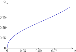
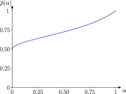
Figure 3. Graph of the function $\alpha\longmapsto\widetilde{\alpha}$ (left-hand side) and graph of the function $\alpha\longmapsto\overline{\rho}(\alpha)$ (right-hand side).

Definition 2.2 (Effective densities).

For any boundary parameter $\alpha\in(0,1)$, define, as represented in Figure 3, the effective active density

$$\widetilde{\alpha}:=\frac{\sqrt{\alpha(4-3\alpha)}-\alpha}{2(1-\alpha)}\in(0,1)$$ (15)

and the effective total particle density

$$\overline{\rho}(\alpha):=\mathfrak{a}^{-1}(\widetilde{\alpha})=\frac{1}{2-\widetilde{\alpha}}\in\big{(}\tfrac{1}{2},1\big{)}.$$ (16)

Remark 2.3.

Note that $\alpha\longmapsto\widetilde{\alpha}$ is an increasing mapping from $[0,1]$ to $[0,1]$. It is easily checked that $\widetilde{\alpha}$ is the only solution in $(0,1)$ of the following identity, which will be used later on,

$$(1-\alpha)\widetilde{\alpha}^{2}=\alpha(1-\widetilde{\alpha}).$$ (17)

We are now ready to define the parameters $\rho_{-}$ and $\rho_{+}$ which appear in the Dirichlet problem (13) in terms of the reservoir densities $\alpha$ and $\beta$.

Definition 2.3 (Dirichlet boundary conditions).

Let $\alpha,\beta\in(0,1)$. Then, the boundary conditions are defined as

$$\rho_{-}:=\overline{\rho}(\alpha)\qquad\mbox{ and }\qquad\rho_{+}:=\overline{\rho}(\beta).$$ (18)

We see that, surprisingly, and unlike for SSEP, equilibrium reservoirs are not able to enforce their own densities to the FEP, because they are not able to enforce subcritical densities, under which the system remains frozen. Rather, equilibrium reservoirs with some density (parameter) $\gamma$, in contact with the FEP, pump particles into the system until they manage to enforce an active density with value $\widetilde{\gamma}>0$. At the macroscopic level, this active density translates into a local density $\overline{\rho}(\gamma)>\frac{1}{2}$. We will explore in details this point later on in Section 3.

2.5. Initial distribution

Although we strongly conjecture that our main result holds in a fairly general setting, in order to focus on the main technical challenges we consider in this article the case of a FEP starting from a supercritical ergodic configuration $\eta$. We therefore need an initial distribution that only charges the ergodic component $\mathcal{E}_{N}$, and that matches an initial density profile. To do so, fix a supercritical continuous initial profile $\rho^{\mathrm{ini}}:[0,1]\to(\frac{1}{2},1]$. For $x\in\llbracket 2,N-1\rrbracket$, we define the associated discrete active density field

$$a_{x}:=\frac{\rho^{\mathrm{ini}}\big{(}\frac{x}{N}\big{)}+\rho^{\mathrm{ini}}\big{(}\frac{x-1}{N}\big{)}-1}{\rho^{\mathrm{ini}}(\frac{x-1}{N}\big{)}}.$$ (19)

Note that $a_{x}\simeq\mathfrak{a}(\rho^{\mathrm{ini}}(\frac{x}{N}))$ as $N\to\infty$. We then define the initial distribution ${\color[rgb]{.15,.0.35,.85}\nu_{0}^{N}}$ for our process as the law of an inhomogeneous Markov chain $(\eta_{x})_{x\in\Lambda_{N}}$ with state-space $\{0,1\}$, started from $\eta_{1}\sim\mathrm{Ber}(\rho^{\mathrm{ini}}(\frac{1}{N}))$, and with transition probabilities

$$\nu_{0}^{N}\big{(}\eta_{x+1}=1\big{|}\eta_{x}=1\big{)}=a_{x+1}\quad\mbox{ and }\quad\nu_{0}^{N}\big{(}\eta_{x+1}=1\big{|}\eta_{x}=0\big{)}=1,$$ (20)

for any $x\in\llbracket 1,N-2\rrbracket$. Note that under those transition probabilities, an empty site is followed by a particle with probability $1$, so that the support of $\nu_{0}^{N}$ is the ergodic component $\mathcal{E}_{N}$. Furthermore, by the Markov property and induction it is immediate to check that for any $x\in\Lambda_{N}$,

$$\nu_{0}^{N}(\eta_{x}=1)=\rho^{\mathrm{ini}}\Big{(}\frac{x}{N}\Big{)}.$$ (21)

We prove in Appendix A.2 that under $\nu_{0}^{N}$, spatial correlations decay exponentially (cf. (135)), therefore by the law of large numbers, $\nu_{0}^{N}$ fits the macroscopic profile $\rho^{\rm ini}$, in the sense that for any smooth function $G$ on $[0,1]$

$$\frac{1}{N}\sum_{x=1}^{N-1}G\Big{(}\frac{x}{N}\Big{)}\eta_{x}\xrightarrow[N\to+\infty]{}\int_{0}^{1}G(u)\rho^{\rm ini}(u)\,\mathrm{d}u$$ (22)

in $\nu_{0}^{N}$-probability.

2.6. Hydrodynamic limit

We are now ready to state our main result.

Theorem 2.4 (Hydrodynamic limit for the boundary-driven FEP).

Let $\alpha,\beta\in(0,1)$, and let $\rho^{\rm ini}:[0,1]\to(\frac{1}{2},1]$ be a continuous initial profile. Recall the initial distribution $\nu_{0}^{N}$ defined in Section 2.5, associated with $\rho^{\rm ini}$.

Then, for all continuous function $G:[0,1]\longrightarrow\mathbb{R}$, $\delta>0$ and $t\in[0,T]$ we have

$$\lim_{N\to+\infty}\mathbb{P}_{\nu_{0}^{N}}\left(\;\left|\;\frac{1}{N}\sum_{x\in\Lambda_{N}}G\Big{(}\frac{x}{N}\Big{)}\eta_{t}(x)-\int_{0}^{1}G(u)\rho_{t}(u)\,\mathrm{d}u\;\right|\;>\delta\right)=0$$ (23)

where $\rho:(t,u)\in[0,T]\times[0,1]\longmapsto\rho_{t}(u)$ is the unique very weak solution (in the sense of Definition 2.1) to the hydrodynamic equation

$$\partial_{t}\rho=\partial_{u}^{2}\mathfrak{a}(\rho),\qquad\rho_{0}=\rho^{\rm ini}$$ (24)

with $\mathfrak{a}$ given by (12), and Dirichlet boundary conditions given by (18), namely

$$\rho_{t}(0)=\overline{\rho}(\alpha),\qquad\rho_{t}(1)=\overline{\rho}(\beta).$$

To conclude this section we briefly explain the strategy of the proof of Theorem 2.4, which is fairly classical. Define the empirical measure

$$m_{t}^{N}(\mathrm{d}u)=\frac{1}{N}\sum_{x\in\Lambda_{N}}\eta_{x}(t)\delta_{\frac{x}{N}}(\mathrm{d}u)$$ (25)

where $\delta_{y}$ stands for the Dirac mass at $y\in[0,1]$. Endowing the space $\mathcal{M}_{+}$ of non-negative measures on $[0,1]$ with the topology of weak convergence of measures, we see that for our choice of initial distribution, $m_{0}^{N}\xrightarrow[N\to+\infty]{}\rho^{\mathrm{ini}}(u)\,\mathrm{d}u$ in probability. Proving the hydrodynamic limit amounts to showing that

$$m_{t}^{N}(\mathrm{d}u)\xrightarrow[N\to+\infty]{}\rho_{t}(u)\,\mathrm{d}u$$

in probability for all $t\in[0,T]$, where $\rho$ is given in Theorem 2.4.

See the empirical measure $m^{N}$ as a mapping from $\mathcal{D}\big{(}[0,T],\Omega_{N}\big{)}$ to $\mathcal{D}\big{(}[0,T],\mathcal{M}_{+}\big{)}$, and denote by $\mathbb{Q}^{N}=\mathbb{P}_{\nu_{0}^{N}}\circ(m^{N})^{-1}$ the pushforward distribution on $\mathcal{D}\big{(}[0,T],\mathcal{M}_{+}\big{)}$ of the empirical measure’s trajectory, corresponding to its law. The strategy of the proof is the following:

1. First, we prove that the sequence $(\mathbb{Q}^{N})_{N\geqslant 1}$ is tight so that we can consider a limit point $\mathbb{Q}$, which can be seen as the law of a random variable $m$ with values in $\mathcal{D}\big{(}[0,T],\mathcal{M}_{+}\big{)}$.

2. Then, we prove that $\mathbb{Q}$ is concentrated on trajectories of measures that are absolutely continuous with respect to the Lebesgue measure. This implies that $m$ writes $m_{t}(\mathrm{d}u)=\rho_{t}(u)\,\mathrm{d}u$ for some density profile $\rho$.

3. Ultimately, we show that this density $\rho$ is a very weak solution (in the sense of Definition 2.1) to the hydrodynamic equation (24). By the uniqueness of very weak solutions, we deduce that the sequence $(\mathbb{Q}^{N})_{N\geqslant 1}$ admits a unique limit point, which is concentrated on the trajectory $\big{(}t\longmapsto\rho_{t}(u)\big{)}$ whose density is the unique very weak solution. It proves that the random variables $(m^{N})_{N\geqslant 1}$ converge in distribution to the trajectory $\big{(}t\longmapsto\rho_{t}(u)\,\mathrm{d}u\big{)}$, and therefore in probability since this limit is deterministic.

Although points (1) and (2) in our context follow straightforwardly from classical arguments [KL99, Chapter 5, Section 1], point (3) above is very delicate in general, and is tackled here using Guo, Papanicolau and Varadhan’s entropy method [GPV88]. The latter is based on replacement lemmas to replace microscopic observables by functions of the empirical measure. Since we are not in a periodic setup, and because the FEP’s invariant states are not product (they charge the ergodic component only), using the entropy method requires understanding the local invariant measure of the process, in particular at the boundaries. This is the first major contribution of our work. The second contribution is the adapation of the entropy method to non-product, non-explicit distributions with strong local correlations.

In the next section, we describe the boundary-driven and infinite volume stationary states for the FEP.

3. Explicit equilibrium states

3.1. Grand-canonical measures on $\mathbb{Z}$

We start by recalling the grand-canonical measures for the facilitated exclusion process in the supercritical phase, that have been studied in details in [BESS20, Section 6.2]. There exists a collection of supercritical reversible probability distributions $(\pi_{\rho})_{\frac{1}{2}<\rho\leqslant 1}$ for the FEP on $\mathbb{Z}$, driven by the generator

$$\mathcal{L}_{\infty}f(\eta)=\sum_{x\in\mathbb{Z}}c_{x,x+1}(\eta)\big{[}f(\eta^{x,x+1})-f(\eta)\big{]},$$ (26)

with the same jump rates given by (3). Those measures are translation invariant, and have support on the (infinite volume) ergodic component ${{\mathcal{E}}}_{\mathbb{Z}}$ (see (10)). Let us fix, for $\ell\geqslant 1$, a box $B_{\ell}:=\llbracket 1,\ell\rrbracket$. Then, given a local configuration $\sigma\in\{0,1\}^{B_{\ell}}$, the grand-canonical states for the FEP are defined by their local marginals

$$\pi_{\rho}\big{(}\eta_{\mid B_{\ell}}=\sigma\big{)}=(1-\rho)(1-\mathfrak{a}(\rho))^{\ell-1-p}\mathfrak{a}(\rho)^{2p-\ell+1-\sigma_{1}-\sigma_{\ell}}\mathds{1}_{\{\sigma\in\mathcal{E}_{B_{\ell}}\}},$$ (27)

where $p={\color[rgb]{.15,.0.35,.85}|\sigma|:=\sum_{x=1}^{\ell}\sigma_{x}}$ is $\sigma$’s number of particles in $B_{\ell}$, and $\mathfrak{a}(\rho)$ is the active density defined in (12).

In practice, this formula is not very convenient for some applications, because it describes $\pi_{\rho}$’s distribution globally in a fixed box rather than sequentially. For this reason, we give the following interpretation of $\pi_{\rho}$: we set $\eta_{0}\sim\mathrm{Ber}(\rho)$, and we define two Markov chains started from $\eta_{0}$, with the same transition probabilities, but the first one, denoted by $(\eta_{x})_{x\geqslant 0}$, goes forward from the origin, while the second one denoted by $(\eta_{-x})_{x\geqslant 0}$, goes backward from the origin (and, once $\eta_{0}$ is chosen, they evolve independently of each other). More precisely we have, for any $x\geqslant 0$,

$$\pi_{\rho}\big{(}\eta_{x+1}=1\big{|}\eta_{x}=1\big{)}=\mathfrak{a}(\rho)\qquad\mbox{ and }\qquad\pi_{\rho}\big{(}\eta_{x+1}=1\big{|}\eta_{x}=0\big{)}=1,$$ (28)

and similarly for the backward chain. As expected, this Markovian construction, starting from an arbitrary site, only charges the ergodic component since as soon as a site is empty, the next one is occupied with probability $1$. It is then straightforward to check that the resulting chain $(\eta_{x})_{x\in\mathbb{Z}}$ has local marginals given by (27), so that its distribution is indeed $\pi_{\rho}$.

Finally, note that the function $\mathfrak{a}(\rho)$ defined in (12) is indeed the active density under $\pi_{\rho}$, since: for any $x\in\mathbb{Z}$,

$$\pi_{\rho}\big{(}h_{x}(\eta)=1\big{)}=\mathfrak{a}(\rho)$$ (29)

where $h_{x}$ was defined in (8) as the indicator function that $x$ is occupied by an active particle.

3.2. Semi-infinite line with one reservoir

Consider now the facilitated exclusion process on the semi-infinite line $\mathbb{N}^{*}$ and in contact with one reservoir of density $\alpha$ at the left boundary, namely a Markov process on $\{0,1\}^{\mathbb{N}^{*}}$ with infinitesimal generator

$$\mathcal{L}_{\ell,\infty}f(\eta)=\mathcal{L}_{\ell}+\sum_{x=1}^{+\infty}c_{x,x+1}(\eta)\big{[}f(\eta^{x,x+1})-f(\eta)\big{]},$$ (30)

where $\mathcal{L}_{\ell}$ has been defined in (5). Once again, for this process, we set $\eta_{0}=1$ so that a particle at the left boundary can always jump to its empty neighbour. It is straighforward to check (adapting Proposition A.1) that the Markov process with generator $\mathcal{L}_{\ell,\infty}$ is irreducible on $\mathcal{E}_{\mathbb{N}^{*}}$. As a consequence, it admits a unique stationary measure $\mu_{\alpha}^{\infty}$ concentrated on the ergodic component $\mathcal{E}_{\mathbb{N}^{*}}$. Given that the infinite volume, grand-canonical measures $\pi_{\rho}$ satisfy a Markovian construction, it is natural to conjecture that $\mu_{\alpha}^{\infty}$ also does. This is indeed the case, and we have the following result.

Proposition 3.1.

The unique stationary measure $\mu_{\alpha}^{\infty}$ of the generator $\mathcal{L}_{\ell,\infty}$ is the distribution of a Markov chain $(\eta_{x})_{x\geqslant 1}$ on $\{0,1\}$, started from $\eta_{1}\sim\mathrm{Ber}(\widetilde{\alpha})$, and with transition probabilities

$$\mu_{\alpha}^{\infty}\big{(}\eta_{x+1}=1\big{|}\eta_{x}=1\big{)}=\widetilde{\alpha}\qquad\mbox{ and }\qquad\mu_{\alpha}^{\infty}\big{(}\eta_{x+1}=1\big{|}\eta_{x}=0\big{)}=1,$$ (31)

where $\widetilde{\alpha}$ is the effective active density defined in (15) .

By stationarity, for any $x\geqslant 1$, $\mu_{\alpha}^{\infty}(\mathcal{L}_{\ell,\infty}\eta_{x})=0$. Therefore, one easily checks that the active density field $\mu_{\alpha}^{\infty}(h_{x}=1)$ is constant equal to $\widetilde{\alpha}$. Then, by the Markov property, the density field

$$\rho_{x}^{\alpha,\infty}:=\mu_{\alpha}^{\infty}(\eta_{x}=1),$$ (32)

represented in Figure 4, satisfies for $x\geqslant 1$ the induction relation

$$\rho^{\alpha,\infty}_{x+1}=\widetilde{\alpha}\rho^{\alpha,\infty}_{x}+1-\rho^{\alpha,\infty}_{x}.$$ (33)

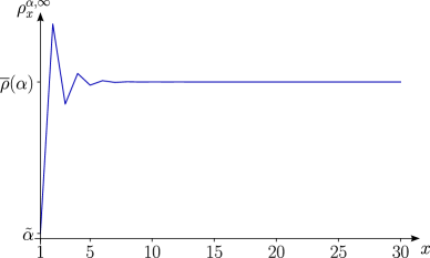
Figure 4. Representation of the profile $x\longmapsto\rho_{x}^{\alpha,\infty}$ on the first thirty sites

Since by construction $\rho^{\alpha,\infty}_{1}=\widetilde{\alpha}$, we obtain by induction the explicit formula: for any $x\geqslant 1$

$$\rho^{\alpha,\infty}_{x}=\frac{1-(\widetilde{\alpha}-1)^{x+1}}{2-\widetilde{\alpha}}=\overline{\rho}(\alpha)+\mathcal{O}(e^{-cx}),$$ (34)

where $c=\log(\widetilde{\alpha}-1)>0$ and $\overline{\rho}(\alpha)$ is given by (15). In other words, an equilibrium reservoir with parameter $\alpha$ imposes an active density $\widetilde{\alpha}$, and, away from the neighbourhood of the boundary, a macroscopic density $\overline{\rho}(\alpha)$. This explains the boundary values (18) appearing in the hydrodynamic limit.

Remark 3.2 (Backward Markov construction).

We chose in Proposition 3.1 to build $\mu_{\alpha}^{\infty}$ going forward, meaning away from the boundary. In this case, the rightwards transition probabilities

$$\overset{\rightarrow}{a}_{x+1}:=\mu_{\alpha}^{\infty}(\eta_{x+1}=1\mid\eta_{x}=1)$$ (35)

are constant equal to $\widetilde{\alpha}$. However, according to Lemma A.3 its finite size marginals can also be built in a Markovian way, going instead towards the boundary, by defining $\mu_{\alpha}^{\infty}(\eta_{1},\dots,\eta_{\ell})$ as follows:

• let $\eta_{\ell}\sim\mathrm{Ber}(\rho^{\alpha,\infty}_{\ell})$ be given by (34) ;

• then, the rest of the configuration is built by enforcing, for $x\in\llbracket 1,\ell-1\rrbracket$, the transition probabilities

  $$\mu_{\alpha}^{\infty}\big{(}\eta_{x}=1\big{|}\eta_{x+1}=1\big{)}=\overset{\leftarrow}{a}_{x}\qquad\mbox{ and }\qquad\mu_{\alpha}^{\infty}\big{(}\eta_{x}=1\big{|}\eta_{x+1}=0\big{)}=1,$$ (36)

  where

  $$\overset{\leftarrow}{a}_{x}:=\frac{\rho^{\alpha,\infty}_{x}+\rho^{\alpha,\infty}_{x+1}-1}{\rho^{\alpha,\infty}_{x+1}}=\widetilde{\alpha}+\frac{\widetilde{\alpha}^{2}-2}{(\widetilde{\alpha}-1)^{-1-x}-\widetilde{\alpha}-1}.$$ (37)

More details are given in Appendix A.3. Note in particular that in this case, the leftwards transition $1\leadsto 1$ given by $\overset{\leftarrow}{a}_{x}$, is not equal to the active density $\widetilde{\alpha}$, in order to account for the finite-size boundary effects.

Remark 3.3 (Uniform bounds on the densities).

Note that, from (34) (see also Figure 4), we have: for any $\alpha\in(0,1)$ and any $x\geqslant 1$

$$0<\widetilde{\alpha}=\rho^{\alpha,\infty}_{1}\leqslant\rho^{\alpha,\infty}_{x}\leqslant\rho^{\alpha,\infty}_{2}<1,$$ (38)

meaning that $\rho^{\alpha,\infty}_{x}$ is bounded away from $0$ and $1$. Using (33), it is easy to check that for any $x\geqslant 0$

$$\overset{\leftarrow}{a}_{x}=\widetilde{\alpha}\;\frac{\rho_{x}^{\alpha,\infty}}{\rho_{x+1}^{\alpha,\infty}},$$ (39)

so that in particular $\overset{\leftarrow}{a}_{x}$ is bounded away from $0$. Finally, since $\rho^{\alpha,\infty}_{x}$ is bounded away from $1$, $(\rho^{\alpha,\infty}_{x}-1)/\rho^{\alpha,\infty}_{x+1}$ is bounded away from $0$, and therefore $\overset{\leftarrow}{a}_{x}$ is also bounded away from $1$. In particular, there exist two constants $0<c<C<1$ such that

$$c<\overset{\leftarrow}{a}_{x}<C\qquad\forall x\geqslant 1.$$ (40)

We now prove Proposition 3.1.

Proof of Proposition 3.1.

First of all, note that by the Markovian construction, the measure defined by (31) is concentrated on the ergodic component $\mathcal{E}_{\mathbb{N}^{*}}$. We will check that this measure is reversible with respect to both the bulk dynamics, and the boundary dynamics. Consider a jump occuring inside the bulk over the edge $(x,x+1)$, this means that the local configuration $(\eta_{x-1},\eta_{x},\eta_{x+1},\eta_{x+2})$ must be either $\bullet$[1pt]$\bullet$$x$$\circ$$\bullet$ or $\bullet$[1pt]$\circ$$x$$\bullet$$\bullet$ (where $\bullet$ stands for a particle and $\circ$ for an empty site), in order for the configuration to be ergodic and to satisfy $c_{x,x+1}(\eta)=1$. The probability under $\mu_{\alpha}^{\infty}$ of observing these two local configurations is respectively $\mu_{\alpha}^{\infty}(\eta_{x-1}=1)\widetilde{\alpha}(1-\widetilde{\alpha})$ and $\mu_{\alpha}^{\infty}(\eta_{x-1}=1)(1-\widetilde{\alpha})\widetilde{\alpha}$. Therefore, since both jumps (back and forth) occur at the same rate $1$, this proves that $\mu_{\alpha}^{\infty}$ is reversible with respect to any FEP jump occuring inside $\{2,3\dots,\}$. The same is true for jumps between sites $1$ and $2$: the latter can only occur if the local configuration $(\eta_{1},\eta_{2},\eta_{3})$ is ergodic and has jump rate $c_{1,2}(\eta)=1$, so it must be given by $\mbox{\stackunder[1pt]{$\bullet$}{\tiny$1$}}\mbox{$\circ$}\mbox{$\bullet$}\cdots$ or $\mbox{\stackunder[1pt]{$\circ$}{\tiny$1$}}\mbox{$\bullet$}\mbox{$\bullet$}\cdots$. The probability of observing these two local configurations is respectively $\widetilde{\alpha}(1-\widetilde{\alpha})$ and $(1-\widetilde{\alpha})\widetilde{\alpha}$, which also proves reversibility with respect to FEP jumps over edge $(1,2)$. In other words, $\mu_{\alpha}^{\infty}$ is reversible with respect to the second part of generator $\mathcal{L}_{\ell,\infty}$ in (30), we now only need to show that it is also reversible with respect to the boundary generator $\mathcal{L}_{\ell}$.

Once again, to ensure that the boundary jump rate is not zero and the configuration is ergodic, the local configuration $(\eta_{1},\eta_{2})$ must be either [1pt]$\bullet$$1$$\bullet$ or [1pt]$\circ$$1$$\bullet$. The probability of the first one is $\widetilde{\alpha}^{2}$, and that of the second one $1-\widetilde{\alpha}$, whereas the transition rate $\mbox{\stackunder[1pt]{$\bullet$}{\tiny$1$}}\mbox{$\bullet$}\mapsto\mbox{\stackunder[1pt]{$\circ$}{\tiny$1$}}\mbox{$\bullet$}$ is $1-\alpha$, and the transition rate $\mbox{\stackunder[1pt]{$\circ$}{\tiny$1$}}\mbox{$\bullet$}\mapsto\mbox{\stackunder[1pt]{$\bullet$}{\tiny$1$}}\mbox{$\bullet$}$ is $\alpha$. Then, identity (17) proves reversibility with respect to the boundary dynamics.∎

3.3. The equilibrium case $\alpha=\beta$

We now get back to our original process in finite volume in contact with two reservoirs, but assume in this section that $\alpha=\beta$. This process has a unique stationary measure $\mu_{\alpha}^{N}$, that is also concentrated on the ergodic component $\mathcal{E}_{N}$. Unfortunately, unlike the semi-infinite case, no Markovian construction holds in the presence of two reservoirs, because the right reservoir has an influence on the left part of the system, preventing a left-right Markovian construction and vice versa. However, we still have an explicit expression analogous to (27), which is uniform over the ergodic configurations with a fixed number of particles. Note that any ergodic configuration $\eta$ on $\Lambda_{N}$ must have at most $k_{N}:=\big{\lceil}\frac{N-1}{2}\big{\rceil}$ empty sites. Denote by $|\mathbf{1}-\eta|=\sum_{x\in\Lambda_{N}}(1-\eta_{x})$ its number of empty sites, and for $0\leqslant k\leqslant k_{N}$, denote by

$$\mathcal{E}_{N}^{k}=\left\{\eta\in\Omega_{N}\;:\;|\mathbf{1}-\eta|=k\mbox{ and }\forall x\in\llbracket 1,N-2\rrbracket,\;\eta_{x}+\eta_{x+1}\geqslant 1\right\}$$

the set of ergodic configurations with $k$ empty sites. Notice that its cardinal is

$$|\mathcal{E}_{N}^{k}|={{N-k}\choose{k}}$$ (41)

because there are $N-k$ possible spots between particles to place the $k$ empty sites.

Proposition 3.4.

The unique stationary measure $\mu_{\alpha}^{N}$ of the generator $\mathcal{L}_{N}$ in the case $\alpha=\beta$ is given by

$$\mu_{\alpha}^{N}(\eta)=\frac{1}{Z_{N}}\sum_{k=0}^{k_{N}}(1-\alpha)^{k}\alpha^{k_{N}-k}\mathds{1}_{\{\eta\in\mathcal{E}_{N}^{k}\}}$$ (42)

for all $\eta\in\Omega_{N}$, where $Z_{N}$ is the renormalizing factor defined by

$$Z_{N}:=\sum_{k=0}^{k_{N}}{{N-k}\choose{k}}(1-\alpha)^{k}\alpha^{k_{N}-k}.$$ (43)

Remark 3.5.

The weight of a configuration under the measure $\mu_{\alpha}^{N}$ can be roughly interpreted as follows: in order to be ergodic, surely we must have $N-1-k_{N}$ particles with probability 1 and then the remaining $k_{N}-k$ particles are inserted with probability $\alpha$ whereas the $k$ holes are inserted with probability $1-\alpha$, no matter their position.

Proof of Proposition 3.4.

With a slight abuse of notation, we denote by $\mu_{\alpha}^{N}$ the measure defined in the statement. Because this measure only charges the ergodic component, any FEP particle jump is reversible, and occurs at rate $1$. Since this bulk dynamics is conservative, it does not change the number of empty sites in the configuration, and since $\mu_{\alpha}^{N}(\eta)$ only depends on the latter, $\mu_{\alpha}^{N}$ is clearly reversible with respect to the bulk dynamics.

We now consider the left boundary dynamics (the right boundary can be treated in the same way). Fix an ergodic configuration $\eta$ with boundary rate $b_{\ell}(\eta)\neq 0$. Then, as in the semi-infinite case the local boundary configuration $(\eta_{1},\eta_{2})$ is either [1pt]$\bullet$$1$$\bullet$ or [1pt]$\circ$$1$$\bullet$, otherwise either $\eta$ is not ergodic, or $b_{\ell}(\eta)=0$. If $(\eta_{1},\eta_{2})=\bullet\bullet$ , the boundary dynamics deletes a particle, so that by (42), $\mu_{\alpha}^{N}(\eta^{1})/\mu_{\alpha}^{N}(\eta)=(1-\alpha)/\alpha$, which is also the ratio between boundary dynamics jump rates by construction. The same applies if $(\eta_{1},\eta_{2})=\circ\bullet$ and proves reversibility. ∎

Define the stationary density profile ${\color[rgb]{.15,.0.35,.85}\rho_{x}^{\alpha,N}:=\mu_{\alpha}^{N}\big{(}\eta_{x}=1\big{)}}$ under $\mu_{\alpha}^{N}$. If we proceed in the same way as before to enumerate the ergodic configurations with $k$ empty sites, and which have a particle at site $x$, we find that

$$\big{|}\mathcal{E}_{N}^{k}\cap\{\eta_{x}=1\}\big{|}=\sum_{i=1}^{x}{{i}\choose{x-i}}{{N-k-i}\choose{k-x+i}}.$$

As a consequence, the density profile is given by

$$\rho_{x}^{\alpha,N}=\frac{1}{Z_{N}}\sum_{k=0}^{k_{N}}\left(\sum_{i=1}^{x}{{i}\choose{x-i}}{{N-k-i}\choose{k-x+i}}\right)(1-\alpha)^{k}\alpha^{k_{N}-k}.$$ (44)

This exact stationary density profile is plotted numerically in Figure 5, and we observe that at both ends it closely matches the one of the semi-infinite system (see Figure 4).

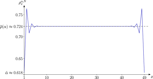
Figure 5. Graph of the profile $x\longmapsto\rho_{x}^{\alpha,N}$ when $\alpha=0.5$ and $N=50$.

We now state some asymptotic properties of this density profile. First, we claim that the equilibrium empirical density is exponentially close to $\overline{\rho}(\alpha)$.

Proposition 3.6.

For $\varepsilon>0$ small enough, there exist constants $K=K(\alpha,\varepsilon)>0$ and $C=C(\alpha,\varepsilon)>0$ such that

$$\mu_{\alpha}^{N}\left(\bigg{|}\frac{|\eta|}{N-1}-\overline{\rho}(\alpha)\bigg{|}>\varepsilon\right)\leqslant Ke^{-CN}.$$

Second, we claim that $\rho_{1}^{\alpha,N}$ and $\rho_{N-1}^{\alpha,N}$ are asymptotically equal to $\widetilde{\alpha}$. Note that this is not true for fixed $N$.

Corollary 3.7.

We have that $\rho_{1}^{\alpha,N}\xrightarrow[N\to+\infty]{}\rho_{1}^{\alpha,\infty}=\widetilde{\alpha}.$

These two results are not necessary to obtain the hydrodynamic limit, however we feel they give an interesting description of the equilibrium case’s stationary states, so that we prove them for the sake of completeness in Appendix A.4.

3.4. The non-equilibrium case $\alpha\neq\beta$

We now get back to the general case where $\alpha\neq\beta$. As in the equilibrium case, there exists a unique stationary measure $\overline{\mu}^{N}$, which cannot satisfy a Markovian construction because of the presence of two reservoirs. In fact, in this non-equilibrium case $\alpha\neq\beta$, due to the presence of long-range correlations already present in the non-equilibrium SSEP, we have no explicit expression for the stationary state. Nevertheless, for all $x\in\llbracket 2,N-2\rrbracket$, we must have

$$0=\overline{\mu}^{N}\big{(}\mathcal{L}_{N}\eta_{x}\big{)}=\overline{\mu}^{N}\big{(}j_{x-1,x}(\eta)-j_{x,x+1}(\eta)\big{)}=\overline{\mu}^{N}\big{(}h_{x-1}(\eta)-2h_{x}(\eta)+h_{x+1}(\eta)\big{)},$$ (45)

where $h_{x}(\eta)$ is defined in (8). As a result, the density of active particles under the measure $\overline{\mu}^{N}$ is affine, and interpolates between the values $\overline{\rho}_{1}^{N}$ and $\overline{\rho}_{N-1}^{N}$ where ${\color[rgb]{0,0,1}\overline{\rho}^{N}_{x}:=\overline{\mu}^{N}(\eta_{x}=1)}$ is the stationary density field, numerically simulated in Figure 6. The reservoirs locally enforce at the boundaries states that look like the semi-infinite case with boundary densities $\alpha$, $\beta$. The next section is dedicated to constructing an explicit approximation $\mu^{N}$ of the measure $\overline{\mu}^{N}$, which locally coincides with $\mu_{\alpha}^{\infty}$ at the left boundary, and with $\mu_{\beta}^{\infty}$ at the right boundary. This approximation will be crucial later on to prove the replacement lemmas in Sections 5.2 and 6.

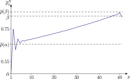
Figure 6. Numerical simulation of the density field $\overline{\rho}^{N}_{x}$ for $N=50$, $\alpha=0.3$ and $\beta=0.8$. Note that the density field is not actually linear in the middle section, but rather of the form $\overline{\rho}_{x}^{N}=1/(2-a_{x})$, where $a_{x}$ is linear.

4. Approximation of the stationary state and Dirichlet form estimates

4.1. Construction of a reference measure $\mu^{N}$

We now construct an approximation of $\overline{\mu}^{N}$ relying on two observations. First, in the transition probabilities (28) and (31) that define the Markovian construction, the probability that an occupied site follows another occupied site is the density of active particles. This is quite intuitive since if site $x$ is occupied, then a particle put at site $x+1$ will automatically be active. The second observation is that the measure $\mu_{\alpha}^{\infty}$ is described by the law of a homogeneous Markov chain that goes from left to right, however, by suitably choosing the transition probabilities as in Remark 3.2, we can also describe it by a non-homogeneous Markov chain from right to left. All that is required to do so is to build a good approximation of the density field in the stationary state, which will in turn yield a good approximation of the stationary distribution, starting from some middlepoint away from the boundaries, and applying the Markov construction forward and backward. To do so, we split the system into three boxes, namely two mesoscopic left and right boundary boxes, and a bulk box. Define ${\color[rgb]{.15,.0.35,.85}x_{N}:=\lfloor\sqrt{N}\rfloor}$, ${\color[rgb]{.15,.0.35,.85}y_{N}:=N-x_{N}}$, and

$$A_{N}:=\llbracket 1,x_{N}\rrbracket\qquad\qquad B_{N}=\rrbracket x_{N},y_{N}\llbracket,\qquad\mbox{ and }\qquad C_{N}=\llbracket y_{N},N-1\rrbracket.$$ (46)

In $A_{N}$, we are at a macroscopic distance of order $1/\sqrt{N}$ of the left boundary, so that the influence of the other reservoir, at macroscopic distance $1$, is not felt. In particular, the density distribution in $A_{N}$ should be close to the one enforced on the semi-infinite line by a reservoir with parameter $\alpha$ and analogously in $C_{N}$ with $\beta$, so we set

$$\rho_{x}^{N}:=\rho_{x}^{\alpha,\infty}\quad\mbox{ for }x\in A_{N},\qquad\mbox{ whereas }\qquad\rho_{x}^{N}:=\rho_{N-x}^{\beta,\infty}\quad\mbox{ for }x\in C_{N}$$ (47)

where $\rho_{x}^{\alpha,\infty}$ was defined in (34).

In particular, we have made sure that our local density profiles at the boundaries are the correct ones. Let us now consider the bulk where the active density should be linear according to (45). We therefore define the active field on $B_{N}$ by setting

$$\overset{\rightarrow}{a}_{x}:=\frac{\widetilde{\beta}-\widetilde{\alpha}}{N}x+\widetilde{\alpha}\qquad\mbox{ for }x\in B_{N}.$$ (48)

Recalling that at site $x_{N}$, the density $\rho_{x_{N}}^{N}=\overline{\rho}(\alpha)+{\mathcal{O}}(e^{-cx_{N}})$ has been defined by (47), we can now define the associated density field on $B_{N}$ by the induction relation

$$\rho_{x}^{N}:=\rho_{x-1}^{N}\overset{\rightarrow}{a}_{x}+1-\rho_{x-1}^{N},\qquad\Longleftrightarrow\qquad\overset{\rightarrow}{a}_{x}:=\frac{\rho^{N}_{x-1}+\rho^{N}_{x}-1}{\rho^{N}_{x-1}},$$ (49)

for $x\in B_{N}$. Equations (47) and (49) define the approximate stationary density field $\rho_{x}^{N}$ on $\Lambda_{N}.$

We now extend our construction of the active density field to $A_{N}$ and $C_{N}$, by setting

$$\overset{\leftarrow}{a}_{x}:=\frac{\rho^{N}_{x+1}+\rho^{N}_{x}-1}{\rho^{N}_{x+1}}\quad\mbox{ for }x\in A_{N}\qquad\mbox{ and }\qquad\overset{\rightarrow}{a}_{x}:=\frac{\rho^{N}_{x-1}+\rho^{N}_{x}-1}{\rho^{N}_{x-1}}\quad\mbox{ for }x\in C_{N},$$ (50)

which together with (48) define two functions $\overset{\leftarrow}{a}_{x}$ for $1\leqslant x<x_{N}$ and $\overset{\rightarrow}{a}_{x}$ for $x_{N}<x<N-1$.

Figure 7. Illustration of the construction of the measure $\mu^{N}$.

We now build our approximated stationary state $\mu^{N}$, by choosing $\eta_{x_{N}}\sim\mathrm{Ber}(\rho_{x_{N}}^{N})$ under $\mu^{N}$. As illustrated in Figure 7, we then apply independently the Markov construction backward and forward, away from $x_{N}$, meaning

$$\mu^{N}\big{(}\eta_{x}=1\big{|}\eta_{x+1}=1\big{)}=\overset{\leftarrow}{a}_{x}\qquad\mbox{ and }\qquad\mu^{N}\big{(}\eta_{x}=1\big{|}\eta_{x+1}=0\big{)}=1\qquad\mbox{ for }1\leqslant x<x_{N},$$ (51)

whereas

$$\mu^{N}\big{(}\eta_{x}=1\big{|}\eta_{x-1}=1\big{)}=\overset{\rightarrow}{a}_{x}\quad\mbox{ and }\quad\mu^{N}\big{(}\eta_{x}=1\big{|}\eta_{x-1}=0\big{)}=1\qquad\mbox{ for }x_{N}<x\leqslant N-1.$$ (52)

This procedure builds a measure $\mu^{N}$ that is concentrated on the ergodic component $\mathcal{E}_{N}$, and is a good candidate to approximate the stationary state $\overline{\mu}^{N}$ of the FEP on $\Lambda_{N}$ in contact with reservoirs with densities $\alpha$ and $\beta$. Following this construction, we obtain the explicit formula

$$\mu^{N}(\eta)=\prod_{x=1}^{x_{N}-1}\Big{(}\eta_{x+1}\overset{\leftarrow}{a}_{x}^{\eta_{x}}(1-\overset{\leftarrow}{a}_{x})^{1-\eta_{x}}+\big{(}1-\eta_{x+1}\big{)}\eta_{x}\Big{)}\\ \times(\rho_{x_{N}}^{N})^{\eta_{x_{N}}}\big{(}1-\rho_{x_{N}}^{N}\big{)}^{1-\eta_{x_{N}}}\times\prod_{x=x_{N}+1}^{N-1}\Big{(}\eta_{x-1}\overset{\rightarrow}{a}_{x}^{\eta_{x}}(1-\overset{\rightarrow}{a}_{x})^{1-\eta_{x}}+\big{(}1-\eta_{x-1}\big{)}\eta_{x}\Big{)}.$$ (53)

Because of the induction relations (49) and (50), it is straightforward to check that the occupancy probability is given by the density field $\rho^{N}$, meaning that for any $x\in\Lambda_{N}$, we have

$$\mu^{N}(\eta_{x}=1)=\rho_{x}^{N}.$$ (54)

In what follows, it will be convenient to define an active density field in the bulk, so that we simplify our notation, and set for all $x\in\Lambda_{N}$

$$a_{x}:=\begin{cases}\overset{\leftarrow}{a}_{x}&\mbox{ if }x\in A_{N}\setminus\{x_{N}\},\\ \widetilde{\alpha}&\mbox{ if }x=x_{N},\\ \overset{\rightarrow}{a}_{x}&\mbox{ if }x\in B_{N}\cup C_{N}.\end{cases}$$ (55)

Note that by construction, the marginal of $\mu^{N}$ with respect to sets $A_{N}$ and $C_{N}$ is exactly the Markov construction (away from the boundary, as described in Remark 3.2) of the semi-infinite equilibrium states $\mu_{\alpha}^{N}$ and $\mu_{\beta}^{N}$.

4.2. Technical estimates on $\mu^{N}$

The rest of this section is dedicated to proving some technical results on this approximate stationary state. We first claim that under $\mu^{N}$, the relation $\rho=1/(2-\mathfrak{a}(\rho))$ between total and active density is asymptotically satisfied in $B_{N}$.

Lemma 4.1.

There exist three constants $C_{1},C_{2}>0$ and $c\in(0,1)$, depending only on $\alpha,\beta$ such that for all $x\in B_{N}$, we have

$$\left|\rho^{N}_{x}-\frac{1}{2-a_{x}}\right|\leqslant\frac{C_{1}c^{x-x_{N}}}{\sqrt{N}}+\frac{C_{2}}{N}.$$ (56)

Proof.

Define

$$\delta_{x}:=\rho^{N}_{x}-\frac{1}{2-a_{x}}.$$ (57)

Using (49), we obtain for $x\in B_{N}$

$$\delta_{x}=1-\rho^{N}_{x-1}+a_{x}\rho^{N}_{x-1}-\frac{1}{2-a_{x}} =\rho^{N}_{x-1}(a_{x}-1)+1-\frac{1}{2-a_{x}}$$

$$=\delta_{x-1}(a_{x}-1)+\frac{a_{x}-1}{2-a_{x-1}}+1-\frac{1}{2-a_{x}}$$

$$=\delta_{x-1}(a_{x}-1)+\frac{a_{x-1}-a_{x}}{(2-a_{x-1})(2-a_{x})}+\frac{a_{x}-a_{x-1}}{2-a_{x-1}}$$

so that

$$|\delta_{x}|\leqslant|\delta_{x-1}||a_{x}-1|+2|a_{x}-a_{x-1}|\leqslant c|\delta_{x-1}|+\frac{2|\widetilde{\beta}-\widetilde{\alpha}|}{N}$$ (58)

because $|a_{x}-1|\leqslant c$ with $c=|\widetilde{\alpha}\wedge\widetilde{\beta}-1|<1$. By induction, we deduce that for $x\in B_{N}$

$$|\delta_{x}|\leqslant c^{x-x_{N}}|\delta_{x_{N}}|+\frac{2|\widetilde{\beta}-\widetilde{\alpha}|}{N}\sum_{k=0}^{x-x_{N}-1}c^{k}\leqslant c^{x-x_{N}}|\delta_{x_{N}}|+\frac{2|\widetilde{\beta}-\widetilde{\alpha}|}{(1-c)N}.$$ (59)

But note that

$$|\delta_{x_{N}}|=\left|\rho_{x_{N}}^{N}-\frac{1}{2-a_{x_{N}}}\right|\leqslant\big{|}\rho_{x_{N}}^{N}-\overline{\rho}(\alpha)\big{|}+\left|\frac{1}{2-\widetilde{\alpha}}-\frac{1}{2-a_{x_{N}}}\right|.$$

The first term on the right-hand side of this inequality is ${\mathcal{O}}(e^{-cx_{N}})$ as noticed in (34), whereas the second term is ${\mathcal{O}}\big{(}\frac{1}{\sqrt{N}}\big{)}$ by the affine expression (48). This proves the result. ∎

We now state that around the junction points $x_{N}$ and $y_{N}$, the local configuration is close to the grand-canonical states $\pi_{\overline{\rho}(\alpha)}$ and $\pi_{\overline{\rho}(\beta)}$ defined in (27), up to a factor ${\mathcal{O}}\big{(}\frac{1}{\sqrt{N}}\big{)}$.

Lemma 4.2.

Fix $\ell\geqslant 1$, there exists a constant $C=C(\alpha,\beta,\ell)>0$ such that for any local configuration $\sigma\in\{0,1\}^{2\ell+1}$,

$$\;\left|\;\mu^{N}(\eta_{|\llbracket x_{N}-\ell,x_{N}+\ell\rrbracket}=\sigma)-\pi_{\overline{\rho}(\alpha)}(\eta_{|\llbracket-\ell,\ell\rrbracket}=\sigma)\;\right|\;\leqslant\frac{C}{\sqrt{N}}$$ (60)

and

$$\;\left|\;\mu^{N}(\eta_{|\llbracket y_{N}-\ell,y_{N}+\ell\rrbracket}=\sigma)-\pi_{\overline{\rho}(\beta)}(\eta_{|\llbracket-\ell,\ell\rrbracket}=\sigma)\;\right|\;\leqslant\frac{C}{\sqrt{N}}.$$ (61)

Proof.

Both distributions can be built by a Markov construction, according to (28), with the difference that $\pi_{\overline{\rho}(\alpha)}$ is started from $\overline{\rho}(\alpha)$, and has backward and forward constant transition rates $a_{x}\equiv\widetilde{\alpha}$ (and similarly for $\pi_{\overline{\rho}(\beta)}$). Assuming that two sequences $u_{k},v_{k}\in(0,1)$ satisfy $|u_{k}-v_{k}|\leqslant\delta$ for $k=1\dots,\ell$, then the difference

$$\;\left|\;\prod_{k=1}^{\ell}u_{k}-\prod_{k=1}^{\ell}v_{k}\;\right|\;\leqslant C_{\ell}\delta$$ (62)

is also of order $\delta$. In particular, recall that $\mu^{N}$ has density $\rho_{x_{N}}^{N}$ at site $x_{N}$ and $\rho_{y_{N}-\ell}^{N}$ at site $y_{N}-\ell$. By the Markovian construction of both $\mu^{N}$ and $\pi_{\rho}$, it is enough to show that for some constant $C$ depending on $\ell$ but not on $N$,

$$|\rho_{x_{N}}^{N}-\overline{\rho}(\alpha)| \leqslant C/\sqrt{N}\qquad\mbox{and}\qquad|\rho_{y_{N}-\ell}^{N}-\overline{\rho}(\beta)|\leqslant C/\sqrt{N},$$ (63)

$$|a_{x}-\widetilde{\alpha}| \leqslant C/\sqrt{N}\qquad\forall x\in\llbracket x_{N}-\ell,x_{N}+\ell\rrbracket\setminus\{x_{N}\},$$ (64)

$$|a_{x}-\widetilde{\beta}| \leqslant C/\sqrt{N}\qquad\forall y\in\rrbracket y_{N}-\ell,y_{N}+\ell\rrbracket.$$ (65)

According to Lemma 4.1 in $B_{N}$, and to (34) in $A_{N}\cup C_{N}$,

$$|\rho_{x}^{N}-\overline{\rho}(\alpha)|\leqslant C/\sqrt{N}\qquad\mbox{and}\qquad|\rho_{y}^{N}-\overline{\rho}(\beta)|\leqslant C/\sqrt{N}$$ (66)

for $x\in\llbracket x_{N}-\ell,x_{N}+\ell\rrbracket$ and $y\in\rrbracket y_{N}-\ell,y_{N}+\ell\rrbracket$. In particular, (64) and (65) follow immediately from the induction relations (49) and (50) and the fact that for $\gamma\in(0,1)$, $\widetilde{\gamma}=(2\overline{\rho}(\gamma)-1)/\overline{\rho}(\gamma)$. ∎

We have a similar result inside the bulk box $B_{N}$, stating that the measure $\mu^{N}$ is locally close to a grand-canonical state.

Lemma 4.3.

Fix $\ell\geqslant 1$, take $u\in\big{(}\frac{x_{N}+\ell}{N},\frac{y_{N}-\ell}{N}\big{)}$ and define $x=\lfloor uN\rfloor\in B_{N}$. Then, there exists a constant $C=C(\alpha,\beta,\ell)>0$ such that for any local configuration $\sigma\in\{0,1\}^{2\ell+1}$, we have

$$\big{|}\mu^{N}(\eta_{|\llbracket x-\ell,x+\ell\rrbracket}=\sigma)-\pi_{\varrho(u)}(\eta_{|\llbracket-\ell,\ell\rrbracket}=\sigma)\big{|}\leqslant\frac{C}{\sqrt{N}}$$ (67)

where

$$\varrho(u):=\frac{1}{2-\big{(}\widetilde{\alpha}+(\widetilde{\beta}-\widetilde{\alpha})u\big{)}}$$ (68)

is the approximated local density around the point $x$ in $\mu^{N}$.

Proof.

As in Lemma 4.2, we only have to prove that

$$|\rho_{x-\ell}^{N}-\varrho(u)| \leqslant\frac{C}{\sqrt{N}},$$ (69)

$$\big{|}a_{y}-\mathfrak{a}\big{(}\varrho(u)\big{)}\big{|} \leqslant\frac{C}{\sqrt{N}}\qquad\forall y\in\rrbracket x-\ell,x+\ell\rrbracket$$ (70)

for some constant $C>0$ that depends only on $\alpha$, $\beta$ and $\ell$. Using Lemma 4.1, one can see that (69) is trivially satisfied. Using the affine expression of $a_{y}$ (see (48)) and the fact that $\mathfrak{a}\big{(}\varrho(u)\big{)}=\widetilde{\alpha}+(\widetilde{\beta}-\widetilde{\alpha})u$, we see that (70) is also satisfied. Note that both hold with constants which are independent of $x$ (thus of $u$). This proves the result. ∎

We now claim that the marginal of $\mu^{N}$ with respect to two distant boxes is roughly a product measure of the local grand-canonical state.

Corollary 4.4.

Fix $\ell\geqslant 1$, there exists a constant $C=C(\alpha,\beta,\ell)>0$ such for any local configurations $\sigma,\sigma^{\prime}\in\{0,1\}^{\ell+1}$, any $x,y\in B_{N}$ satisfying

$$x_{N}+(\log N)^{2}\leqslant x<y\leqslant y_{N}-(\log N)^{2}\qquad\mbox{ and }\qquad y-x>(\log N)^{2},$$ (71)

we have

$$\;\left|\;\mu^{N}(\eta_{|\llbracket x,x+\ell\rrbracket}=\sigma,\;\eta_{|\llbracket y,y+\ell\rrbracket}=\sigma^{\prime})-\pi_{\rho_{x}^{N}}(\eta_{|\llbracket 0,\ell\rrbracket}=\sigma)\pi_{\rho_{y}^{N}}(\eta_{|\llbracket 0,\ell\rrbracket}=\sigma^{\prime})\;\right|\;\leqslant\frac{C}{N}.$$ (72)

Proof.

Thanks to (40) and (48), we see that the density field $(a_{x})_{x\in\Lambda_{N}}$ is bounded away from 0. The proof of this corollary is then straightforward thanks to the decorrelation estimate given in Theorem A.2, which yields, since $y-x>(\log N)^{2}$, that

$$|\mu^{N}(\eta_{|\llbracket x,x+\ell\rrbracket}=\sigma,\;\eta_{|\llbracket y,y+\ell\rrbracket}=\sigma^{\prime})-\mu^{N}(\eta_{|\llbracket x,x+\ell\rrbracket}=\sigma)\mu^{N}(\eta_{|\llbracket y,y+\ell\rrbracket}=\sigma^{\prime})|\leqslant\frac{C}{N}.$$ (73)

We can then use exactly the same arguments as in Lemma 4.2 to compare the Markovian constructions of $\mu^{N}(\eta_{|\llbracket x,x+\ell\rrbracket}=\sigma)$ and $\pi_{\rho_{x}^{N}}(\eta_{|\llbracket x,x+\ell\rrbracket}=\sigma)$, and use Lemma 4.1 to obtain that for any $x^{\prime}\in\llbracket x,x+\ell\rrbracket$

$$|\rho^{N}_{x^{\prime}}-\rho_{x}^{N}|={\mathcal{O}}\Big{(}\frac{\ell}{N}\Big{)}\qquad\mbox{ and }\qquad\left|a_{x^{\prime}}-\frac{2\rho_{x}^{N}-1}{\rho_{x}^{N}}\right|={\mathcal{O}}\Big{(}\frac{\ell}{N}\Big{)},$$ (74)

uniformly in $x\geqslant x_{N}+(\log N)^{2}$. The same is true in $\llbracket y,y+\ell\rrbracket$, with $\rho_{y}^{N}$ replacing $\rho_{x}^{N}$ which yields Corollary 4.4. ∎

We finally show that our reference measure is regular enough in an entropic sense. Given two probability measures $\nu$, $\mu$ on $\Omega_{N},$ define the relative entropy

$$H(\nu|\mu)=\sum_{\eta\in\Omega_{N}}\nu(\eta)\log\left(\frac{\nu(\eta)}{\mu(\eta)}\right)=\mathbb{E}_{\mu}\left(\frac{\,\mathrm{d}\nu}{\,\mathrm{d}\mu}\log\frac{\,\mathrm{d}\nu}{\,\mathrm{d}\mu}\right).$$ (75)

We now give a crude entropy bound with respect to our approximate stationary state $\mu^{N}$.

Lemma 4.5.

There exists a constant $C_{0}=C_{0}(\alpha,\beta)>0$ such that for any probability measure $\nu$ which is concentrated on the ergodic component $\mathcal{E}_{N}$, we have

$$H(\nu|\mu^{N})\leqslant C_{0}N.$$

Proof.

According to (40) and (48), there exists two constants $0<c^{\prime}<C^{\prime}<1$ such that

$$\forall x\in\Lambda_{N},\qquad c^{\prime}\leqslant a_{x}\leqslant C^{\prime}.$$ (76)

Using these bounds in (53) yields that for any ergodic configuration $\eta\in\mathcal{E}_{N}$, we have

$$\mu^{N}(\eta) \geqslant\big{(}c^{\prime}\wedge(1-C^{\prime})\big{)}^{x_{N}-1}\times\Big{(}\overline{\rho}(\alpha)\wedge\big{(}1-\overline{\rho}(\alpha)\big{)}\Big{)}\times\big{(}c^{\prime}\wedge(1-C^{\prime})\big{)}^{N-x_{N}}$$

$$\geqslant\frac{1}{2}\big{(}c^{\prime}\wedge(1-C^{\prime})\big{)}^{N-2}.$$

In particular, since $\nu(\eta)\leqslant 1$, we have $\log\big{(}\frac{\,\mathrm{d}\nu}{\,\mathrm{d}\mu}\big{)}\leqslant C_{0}(N-2)$, thus proving the lemma. ∎

4.3. Dirichlet estimate

Fix a function $f:\Omega_{N}\rightarrow\mathbb{R}$, define the Dirichlet form with respect to $\mu^{N}$ as

$$\mathfrak{D}_{N}(f)=\underbrace{\sum_{x=1}^{N-2}\mathfrak{D}_{0}^{x}(f)}_{\displaystyle=:\mathfrak{D}_{0}(f)}+\mathfrak{D}_{\ell}(f)+\mathfrak{D}_{r}(f)$$ (77)

where

$$\mathfrak{D}_{0}^{x}(f) =\int_{\Omega_{N}}c_{x,x+1}(\eta)\big{[}\sqrt{f(\eta^{x,x+1})}-\sqrt{f(\eta)}\big{]}^{2}\,\mathrm{d}\mu^{N}(\eta)$$ (78a)

$$\mathfrak{D}_{\ell}(f) =\int_{\Omega_{N}}b_{\ell}(\eta)\big{[}\sqrt{f(\eta^{1})}-\sqrt{f(\eta)}\big{]}^{2}\,\mathrm{d}\mu^{N}(\eta)$$ (78b)

$$\mathfrak{D}_{r}(f) =\int_{\Omega_{N}}b_{r}(\eta)\big{[}\sqrt{f(\eta^{N-1})}-\sqrt{f(\eta)}\big{]}^{2}\,\mathrm{d}\mu^{N}(\eta)$$ (78c)

and the bulk and boundary rates have been defined in (3) and (6). Thanks to the technical estimates obtained in the previous section, we are in a position to estimate the spectral radius of the generator $\mathcal{L}_{N}$ with the Dirichlet form $\mathfrak{D}_{N}$.

Proposition 4.6.

There exists a constant $C=C(\alpha,\beta)>0$ such that for any density $f:\Omega_{N}\longrightarrow[0,+\infty]$ with respect to the measure $\mu^{N}$, we have

$$\mu^{N}(\sqrt{f}\mathcal{L}_{N}\sqrt{f})\leqslant-\frac{1}{4}\mathfrak{D}_{N}(f)+\frac{C}{N}.$$ (79)

To prove this estimate, we will use repeatedly the following classical estimate, whose proof can be found in [BGJO19, Lemma 5.1].

Lemma 4.7.

Let $T:\eta\mapsto T_{\eta}\in\Omega_{N}$ be a configuration transformation, and let $c:\Omega_{N}\longrightarrow[0,+\infty[$ be a non-negative local function. Let $f$ be a density with respect to a probability measure $\mu$. Then, we have that

$$\int_{\Omega_{N}}c(\eta)\big{[}\sqrt{f(T_{\eta})}-\sqrt{f(\eta)}\big{]}\sqrt{f(\eta)}\,\mathrm{d}\mu(\eta)\\ \leqslant-\frac{1}{4}\int_{\Omega_{N}}c(\eta)\big{[}\sqrt{f(T_{\eta})}-\sqrt{f(\eta)}\big{]}^{2}\,\mathrm{d}\mu(\eta)+\frac{1}{8}\int_{\Omega^{\mu c}_{N}}c(\eta)\left(1-\frac{c(T_{\eta})}{c(\eta)}\frac{\mu(T_{\eta})}{\mu(\eta)}\right)^{2}[f(T_{\eta})+f(\eta)]\,\mathrm{d}\mu(\eta),$$ (80)

where we defined $\Omega^{\mu c}_{N}:=\{\eta\in\Omega_{N}:\;\mu c(\eta)>0\}$.

Proof of Proposition 4.6.

The quantity in the left-hand side of (79) is a sum of three terms, each one coming from one of the generators $\mathcal{L}_{0}$, $\mathcal{L}_{\ell}$ and $\mathcal{L}_{r}$. Let us treat each of these terms separately, beginning with the term associated to the generator $\mathcal{L}_{0}$. By definition, it writes

$$\mu^{N}(\sqrt{f}\mathcal{L}_{0}\sqrt{f}) =\sum_{x=1}^{N-2}\int_{\Omega_{N}}c_{x,x+1}(\eta)\big{[}\sqrt{f(\eta^{x,x+1})}-\sqrt{f(\eta)}\big{]}\sqrt{f(\eta)}\,\mathrm{d}\mu^{N}(\eta)$$

$$=\sum_{x=1}^{N-2}\int_{\Omega^{x}_{N}}\big{[}\sqrt{f(\eta^{x,x+1})}-\sqrt{f(\eta)}\big{]}\sqrt{f(\eta)}\,\mathrm{d}\mu^{N}(\eta)$$

where we defined

$$\Omega_{N}^{x}=\Omega^{\mu^{N}c_{x,x+1}}_{N}:=\{\eta\in\mathcal{E}_{N}\;:\;c_{x,x+1}(\eta)=1\}.$$ (81)

We now apply Lemma 4.7 with $c\equiv 1$ and $\mu=\mu^{N}$ to each of these integrals, we obtain

$$\mu^{N}(\sqrt{f}\mathcal{L}_{0}\sqrt{f})\leqslant-\frac{1}{4}\mathfrak{D}_{0}(f)+\frac{1}{8}\sum_{x=1}^{N-2}\int_{\Omega_{N}^{x}}\left(1-\frac{\mu^{N}(\eta^{x,x+1})}{\mu^{N}(\eta)}\right)^{2}\big{[}f(\eta^{x,x+1})+f(\eta)\big{]}\,\mathrm{d}\mu^{N}(\eta).$$ (82)

Denote by $\{\mbox{$\bullet$}\mbox{\stackunder[1pt]{$\bullet$}{\tiny$x$}}\mbox{$\circ$}\mbox{$\bullet$}\}$ the event $\{\eta\in\mathcal{E}_{N},\;(\eta_{x-1},\eta_{x},\eta_{x+1},\eta_{x+2})=(1,1,0,1)\}$, and similarly we write $\{\mbox{$\bullet$}\mbox{\stackunder[1pt]{$\circ$}{\tiny$x$}}\mbox{$\bullet$}\mbox{$\bullet$}\}$ for the event $\{\eta\in\mathcal{E}_{N},\;(\eta_{x-1},\eta_{x},\eta_{x+1},\eta_{x+2})=(1,0,1,1)\}$. Then, one easily checks that $\Omega_{N}^{x}=\{\mbox{$\bullet$}\mbox{\stackunder[1pt]{$\bullet$}{\tiny$x$}}\mbox{$\circ$}\mbox{$\bullet$}\}\cup\{\mbox{$\bullet$}\mbox{\stackunder[1pt]{$\circ$}{\tiny$x$}}\mbox{$\bullet$}\mbox{$\bullet$}\}$, and clearly $\{\mbox{$\bullet$}\mbox{\stackunder[1pt]{$\bullet$}{\tiny$x$}}\mbox{$\circ$}\mbox{$\bullet$}\}=\{\eta^{x,x+1},\;\eta\in${$\bullet$[1pt]$\circ$$x$$\bullet$$\bullet$}$\}$. Furthermore, because of the Markovian construction, we have

$$\mu^{N}\big{(}\eta_{y},y\notin\llbracket x-1,x+2\rrbracket\;\big{|}\;\mbox{$\bullet$}\mbox{\stackunder[1pt]{$\bullet$}{\tiny$x$}}\mbox{$\circ$}\mbox{$\bullet$}\big{)}=\mu^{N}\big{(}\eta_{y},y\notin\llbracket x-1,x+2\rrbracket\;\big{|}\;\mbox{$\bullet$}\mbox{\stackunder[1pt]{$\circ$}{\tiny$x$}}\mbox{$\bullet$}\mbox{$\bullet$}\big{)},$$ (83)

because the only influence of the configuration in $\llbracket x-1,x+2\rrbracket$ on the configuration outside is through the extremities $x-1$ and $x+2$, which are both occupied in $\{\mbox{$\bullet$}\mbox{\stackunder[1pt]{$\bullet$}{\tiny$x$}}\mbox{$\circ$}\mbox{$\bullet$}\}$ and $\{\mbox{$\bullet$}\mbox{\stackunder[1pt]{$\circ$}{\tiny$x$}}\mbox{$\bullet$}\mbox{$\bullet$}\}$. This allows us to obtain from (82) the bound

$$\mu^{N}(\sqrt{f}\mathcal{L}_{0}\sqrt{f})\leqslant-\frac{1}{4}\mathfrak{D}_{0}(f)+\frac{1}{8\gamma^{2}}\sum_{x=1}^{N-2}\int_{\Omega_{N}^{x}}\Big{(}\mu^{N}(\mbox{$\bullet$}\mbox{\stackunder[1pt]{$\bullet$}{\tiny$x$}}\mbox{$\circ$}\mbox{$\bullet$})-\mu^{N}(\mbox{$\bullet$}\mbox{\stackunder[1pt]{$\circ$}{\tiny$x$}}\mbox{$\bullet$}\mbox{$\bullet$})\Big{)}^{2}\big{[}f(\eta^{x,x+1})+f(\eta)\big{]}\,\mathrm{d}\mu^{N}(\eta).$$ (84)

since by (38) and (40) both $\mu^{N}(\mbox{$\bullet$}\mbox{\stackunder[1pt]{$\bullet$}{\tiny$x$}}\mbox{$\circ$}\mbox{$\bullet$})$ and $\mu^{N}(\mbox{$\bullet$}\mbox{\stackunder[1pt]{$\circ$}{\tiny$x$}}\mbox{$\bullet$}\mbox{$\bullet$})$ are bounded from below by a positive constant $\gamma>0$ uniformly in $x$ and $N$.

We now only have to estimate, for all $x\in\llbracket 1,N-2\rrbracket$, the difference

$$\delta_{x}:=\big{|}\mu^{N}(\mbox{$\bullet$}\mbox{\stackunder[1pt]{$\bullet$}{\tiny$x$}}\mbox{$\circ$}\mbox{$\bullet$})-\mu^{N}(\bullet\mbox{\stackunder[1pt]{$\circ$}{\tiny$x$}}\mbox{$\bullet$}\mbox{$\bullet$})\big{|}.$$ (85)

For $x\leqslant x_{N}-3$ or $x\geqslant y_{N}+3$, we have $\delta_{x}=0$ because the marginal of $\mu^{N}$ with respect to $(\eta_{x-1},\eta_{x},\eta_{x+1},\eta_{x+2})$ is exactly the semi-infinite stationnary state (either $\mu_{\alpha}^{\infty}$ or $\mu_{\beta}^{\infty}$), which is reversible with respect to any particle jump (cf. Proposition 3.1). For $x\in\llbracket x_{N}+1,y_{N}-2\rrbracket$, we are far enough from the junction points in the bulk, so that

$$\delta_{x}=\big{|}\rho^{N}_{x-1}a_{x}(1-a_{x+1})-\rho^{N}_{x-1}(1-a_{x})a_{x+2}\big{|}=\rho^{N}_{x-1}\left|\frac{(2-a_{x})(\widetilde{\beta}-\widetilde{\alpha})}{N}\right|={\mathcal{O}}\Big{(}\frac{1}{N}\Big{)}$$

thanks to the affine expression (48) for $a_{y}$. Finally, for $x\in\llbracket x_{N}-2,x_{N}\rrbracket$ (resp. $x\in\llbracket y_{N}-1,y_{N}+2\rrbracket$) according to Lemma 4.2 with $\ell=2$, up to an error term of order $1/\sqrt{N}$, both probabilities are equal to

$$\pi_{\overline{\rho}(\alpha)}(\mbox{$\bullet$}\mbox{\stackunder[1pt]{$\bullet$}{\tiny$x$}}\mbox{$\circ$}\mbox{$\bullet$})=\pi_{\overline{\rho}(\alpha)}(\mbox{$\bullet$}\mbox{\stackunder[1pt]{$\circ$}{\tiny$x$}}\mbox{$\bullet$}\mbox{$\bullet$})=\overline{\rho}(\alpha)(1-\widetilde{\alpha})\widetilde{\alpha}$$ (86)

(resp. $\overline{\rho}(\beta)(1-\widetilde{\beta})\widetilde{\beta}$), therefore in those cases $\delta_{x}={\mathcal{O}}(1/\sqrt{N})$.

Since $f$ is a density with respect to $\mu^{N}$, and since $\mu^{N}(\eta^{x,x+1})/\mu^{N}(\eta)$ is bounded by construction, the integral $\int_{\Omega_{N}^{x}}f(\eta^{x,x+1})\,\mathrm{d}\mu^{N}(\eta)$ is bounded uniformly in $x$ as well. Injecting the previous estimates of $\delta_{x}$ in (84) then yields as wanted that for some constant $C$ depending only on $\alpha$ and $\beta$

$$\mu^{N}(\sqrt{f}\mathcal{L}_{0}\sqrt{f})\leqslant-\frac{1}{4}\mathfrak{D}_{0}(f)+\frac{C}{N}.$$ (87)

Let us now deal with the term coming from the generator ${\mathcal{L}}_{\ell}$ of the left boundary. A similar application of Lemma 4.7 yields that

$$\mu^{N}(\sqrt{f}{\mathcal{L}}_{\ell}\sqrt{f})\leqslant-\frac{1}{4}\mathfrak{D}_{\ell}(f)+\frac{1}{8}\int_{\Omega_{N}^{0}}b_{\ell}(\eta)\left(1-\frac{b_{\ell}(\eta^{1})}{b_{\ell}(\eta)}\frac{\mu^{N}(\eta^{1})}{\mu^{N}(\eta)}\right)^{2}\big{[}f(\eta^{1})+f(\eta)\big{]}\,\mathrm{d}\mu^{N}(\eta)$$ (88)

where $\Omega_{N}^{0}:=\Omega_{N}^{\mu^{N}b_{\ell}}$. In $\Omega_{N}^{0}$, there are only two possible configurations on $\{1,2\}$, namely [1pt]$\bullet$$1$$\bullet$ and [1pt]$\circ$$1$$\bullet$ and we go from one to the other by the transformation $\eta\longmapsto\eta^{1}$. But note that

$$b_{\ell}(\mbox{\stackunder[1pt]{$\circ$}{\tiny$1$}}\mbox{$\bullet$})\mu^{N}(\mbox{\stackunder[1pt]{$\circ$}{\tiny$1$}}\mbox{$\bullet$})-b_{\ell}(\mbox{\stackunder[1pt]{$\bullet$}{\tiny$1$}}\mbox{$\bullet$})\mu^{N}(\mbox{\stackunder[1pt]{$\bullet$}{\tiny$1$}}\mbox{$\bullet$})=\alpha(1-\widetilde{\alpha})-(1-\alpha)\widetilde{\alpha}^{2}=0$$

since $\mu^{N}$ coincides with the measure $\mu_{\alpha}^{N}$ on left boundary, and using the relation (17). As a consequence, the integral on the right-hand side of (88) vanishes and

$$\mu^{N}(\sqrt{f}{\mathcal{L}}_{\ell}\sqrt{f})\leqslant-\frac{1}{4}\mathfrak{D}_{\ell}(f).$$ (89)

The term coming from the generator ${\mathcal{L}}_{r}$ of the right boundary can be treated in the exact same way to get that

$$\mu^{N}(\sqrt{f}{\mathcal{L}}_{r}\sqrt{f})\leqslant-\frac{1}{4}\mathfrak{D}_{r}(f).$$ (90)

Putting (87), (89) and (90) together, we deduce the result. ∎

5. Proof of Theorem 2.4

5.1. Dynkin’s martingale and replacement lemmas

We now have the main ingredients needed to carry on with the proof of the hydrodynamic limit. Recall that we defined in Section 2.6 the distribution $\mathbb{Q}^{N}=\mathbb{P}_{\nu_{0}^{N}}\circ(m^{N})^{-1}$ of the boundary-driven FEP empirical measure’s trajectory. The proof of the tightness of $(\mathbb{Q}^{N})_{N\geqslant 1}$ is very standard and relies on Aldous criterion which gives a necessary and sufficient condition for a sequence of measures to be tight in the Skorokhod topology, we omit it and we refer the reader to [KL99, Section 4.2]. Since we are dealing with an exclusion process, following classical arguments (see e.g. [KL99, page 57]), it is straightforward to show that any limit point of $(\mathbb{Q}^{N})_{N\geqslant 1}$ is concentrated on trajectories $(m_{t})_{t\geqslant 0}$ which are absolutely continuous with respect to the Lebesgue measure and write $m_{t}(\mathrm{d}u)=\rho_{t}(u)\mathrm{d}u$, where the profile $\rho_{t}(\cdot)$ takes its values in $[0,1]$.

We now prove that the density $\rho$ of the limiting measure $m$ is a weak solution to the hydrodynamic equation (24). This part of the proof is also classical, we sketch it for completeness, before turning to the replacement lemmas that require more attention. By construction, as detailed in Section 2.5 at time $t=0$, this density coincides with the chosen initial profile, meaning that any limit point $\mathbb{Q}$ of $(\mathbb{Q}^{N})_{N\geqslant 1}$ satisfies that for all $\delta>0$, and all continuous function $G:[0,1]\longrightarrow\mathbb{R}$,

$$\mathbb{Q}\left(\left|\langle m_{0},G\rangle-\int_{0}^{1}\rho^{\mathrm{ini}}(u)G(u)\,\mathrm{d}u\right|>\delta\right)=0$$ (91)

by (22). Fix a test function $G\in\mathcal{C}_{0}^{1,2}\big{(}[0,T]\times[0,1]\big{)}$, it is well-known (see [KL99, Lemma 5.1, Appendix 1.5]) that

$${\mathbb{M}}_{t}^{N}(G):=\langle m_{t}^{N},G_{t}\rangle-\langle m_{0}^{N},G_{0}\rangle-\int_{0}^{t}\langle m_{s}^{N},\partial_{t}G_{s}\rangle\,\mathrm{d}s-\int_{0}^{t}N^{2}\mathcal{L}_{N}\langle m_{s}^{N},G_{s}\rangle\,\mathrm{d}s$$ (92)

is a mean-zero martingale with quadratic variation bounded by ${\mathcal{O}}\big{(}\frac{1}{N}\big{)}$, and therefore vanishes in $L^{2}$ as $N$ goes to infinity.

Recall that we defined the instantaneous current through the bond $\{x,x+1\}\subset\Lambda_{N}$ in the configuration $\eta$ by

$$j_{x,x+1}(\eta)=c_{x,x+1}(\eta)\big{(}\eta_{x}-\eta_{x+1}\big{)}=h_{x}(\eta)-h_{x+1}(\eta)$$ (93)

where $c_{x,x+1}$ has been defined in (3) and $h_{x}$ in (8). We further define the instantaneous current through the “reservoir bonds” $\{0,1\}$ and $\{N-1,N\}$ respectively by

$$j_{0,1}(\eta)=b_{\ell}(\eta)\big{(}1-2\eta_{1}\big{)}\qquad\mbox{ and }\qquad j_{N-1,N}(\eta)=b_{r}(\eta)\big{(}2\eta_{N-1}-1\big{)},$$ (94)

where $b_{\ell}$ and $b_{r}$ are the boundary rates defined in (6). With these definitions, if we apply the generator $\mathcal{L}_{N}$ to the local function $\eta\longmapsto\eta_{x}$ we have that

$$\mathcal{L}_{N}\eta_{x}=j_{x-1,x}(\eta)-j_{x,x+1}(\eta)$$

for all $x\in\Lambda_{N}$. Recall that for a function $g(\eta)$, we simply write $g(s):=g(\eta(s))$. As a consequence, after two successive summations by parts, the term inside the second integral of (92) writes

$$N^{2}\mathcal{L}_{N}\langle m_{s}^{N},G_{s}\rangle=NG_{s}\Big{(}\frac{1}{N}\Big{)}j_{0,1}(s)-NG_{s}\Big{(}\frac{N-1}{N}\Big{)}j_{N-1,N}(s)\\ +\nabla_{N}^{+}G_{s}(0)h_{1}(s)-\nabla_{N}^{-}G_{s}(1)h_{N-1}(s)+\frac{1}{N}\sum_{x\in\Lambda_{N}}\Delta_{N}G_{s}\Big{(}\frac{x}{N}\Big{)}h_{x}(s)$$

where we defined the discrete gradients by

$$\nabla_{N}^{+}G\Big{(}\frac{x}{N}\Big{)}=N\left(G\Big{(}\frac{x+1}{N}\Big{)}-G\Big{(}\frac{x}{N}\Big{)}\right)\quad\mbox{ and }\quad\nabla_{N}^{-}G\Big{(}\frac{x}{N}\Big{)}=N\left(G_{s}\Big{(}\frac{x}{N}\Big{)}-G\Big{(}\frac{x-1}{N}\Big{)}\right),$$

and the discrete Laplacian by

$$\Delta_{N}G\Big{(}\frac{x}{N}\Big{)}=N^{2}\left(G\Big{(}\frac{x+1}{N}\Big{)}+G\Big{(}\frac{x-1}{N}\Big{)}-2G\Big{(}\frac{x}{N}\Big{)}\right).$$

Since we set $\eta_{0}=\eta_{N}\equiv 1$, $h_{1}(\eta)=\eta_{1}$ and $h_{N-1}(\eta)=\eta_{N-1}$. This, together with the fact that $G$ vanishes at the boundaries for all time, allows to rewrite Dynkin’s martingale under the form

$${\mathbb{M}}_{t}^{N}(G)=\langle m_{t}^{N},G_{t}\rangle-\langle m_{0}^{N},G_{0}\rangle-\int_{0}^{t}\langle m_{s}^{N},\partial_{t}G_{s}\rangle\,\mathrm{d}s-\int_{0}^{t}\frac{1}{N}\sum_{x\in\Lambda_{N}}\Delta_{N}G_{s}\Big{(}\frac{x}{N}\Big{)}h_{x}(s)\,\mathrm{d}s\\ -\int_{0}^{t}\Big{\{}\nabla_{N}^{+}G_{s}(0)\big{(}\eta_{1}(s)+j_{0,1}(s)\big{)}-\nabla_{N}^{-}G_{s}(1)\big{(}\eta_{N-1}(s)-j_{N-1,N}(s)\big{)}\Big{\}}\,\mathrm{d}s.$$ (95)

To obtain the weak formulation (14), we need to replace local functions of the configuration by functions of the empirical measure. Our first replacement lemma states that, as $N\to+\infty$, the terms $\eta_{1}(s)$ and $\eta_{N-1}(s)$ appearing in (95) can be replaced by their limiting expected value under the stationary state, namely $\widetilde{\alpha}$ or $\widetilde{\beta}$ (cf. Corollary 3.7).

Lemma 5.1.

For all $t\in[0,T]$, and for all $\mathcal{C}^{1}$ function $\varphi:[0,T]\longrightarrow\mathbb{R}$, we have

$$\lim_{N\to+\infty}\mathbb{E}_{\nu_{0}^{N}}\left[\bigg{|}\int_{0}^{t}\varphi(s)\big{(}\eta_{1}(s)-\widetilde{\alpha}\big{)}\,\mathrm{d}s\bigg{|}\right]=0$$ (96)

where $\widetilde{\alpha}$ has been defined by (15). The same holds true if we replace $\eta_{1}(s)$ by $\eta_{N-1}(s)$ and $\widetilde{\alpha}$ by $\widetilde{\beta}$ in this expression.

The second replacement lemma says that the instantaneous currents $j_{0,1}$ and $j_{N-1,N}$ appearing in (95) vanish in the limit $N\to+\infty$.

Lemma 5.2.

For all $t\in[0,T]$, and for all $\mathcal{C}^{1}$ function $\varphi:[0,T]\longrightarrow\mathbb{R}$, we have

$$\lim_{N\to+\infty}\mathbb{E}_{\nu_{0}^{N}}\left[\bigg{|}\int_{0}^{t}\varphi(s)j_{0,1}(s)\,\mathrm{d}s\bigg{|}\right]=0.$$ (97)

The same holds true if we replace $j_{0,1}$ by $j_{N-1,N}$ in this expression.

We prove these two lemmas in Section 5.2. To close (95) with respect to the empirical measure, we need a last replacement lemma. Take $\varepsilon>0$ and recall the definition of the active density $\mathfrak{a}(\rho)$ at density $\rho$ given in (12). This last lemma asserts that we can replace each $h_{x}(s)$ in (95) by $\mathfrak{a}\big{(}\eta_{x}^{\varepsilon N}(s)\big{)}$, wherever

$$\eta_{x}^{\varepsilon N}(s):=\frac{1}{2\varepsilon N}\sum_{|y|\leqslant\varepsilon N}\eta_{x+y}(s)$$ (98)

is well-defined, that is for all $x\in{\color[rgb]{.15,.0.35,.85}\Sigma_{N}^{\varepsilon}:=\llbracket 1+\varepsilon N,(1-\varepsilon)N-1\rrbracket}$. More precisely, Lemma 5.3 below says that the error that we make when we do this replacement vanishes when we let $N$ go to $+\infty$, and then $\varepsilon$ to 0:

Lemma 5.3.

For any $t\in[0,T]$, and for any continuous function $\varphi:[0,T]\times[0,1]\longrightarrow\mathbb{R}$ we have that

$$\limsup_{\varepsilon\to 0}\limsup_{N\to+\infty}\mathbb{E}_{\nu_{0}^{N}}\left[\bigg{|}\int_{0}^{t}\frac{1}{N}\sum_{x\in\Sigma_{N}^{\varepsilon}}\varphi_{s}\Big{(}\frac{x}{N}\Big{)}\big{(}h_{x}(s)-\mathfrak{a}\big{(}\eta_{x}^{\varepsilon N}(s)\big{)}\big{)}\,\mathrm{d}s\bigg{|}\right]=0.$$ (99)

Note that we only prove the replacement for $x\in\Sigma_{N}^{\varepsilon}$, because for any smooth $G$

$$\int_{0}^{t}\frac{1}{N}\sum_{x\in\Lambda_{N}\setminus\Sigma_{N}^{\varepsilon}}\Delta_{N}G_{s}\Big{(}\frac{x}{N}\Big{)}h_{x}(\eta_{s})\,\mathrm{d}s\underset{\varepsilon\to 0}{=}\mathcal{O}(\varepsilon).$$ (100)

The proof of Lemma 5.3 has to be carefully adapted from the proof of [BESS20, Lemma 5.4] because the addition of boundary dynamics and the nature of the FEP’s stationary states breaks down some translation invariance-based arguments. We postpone it to Section 6, and now complete the proof of the hydrodynamic limit. Note that $\eta_{x}^{\varepsilon N}(s)=m_{s}^{N}*\iota_{\varepsilon}\big{(}\frac{x}{N}\big{)}$, where $\iota_{\varepsilon}=\frac{1}{2\varepsilon}\mathds{1}_{[-\varepsilon,\varepsilon]}$ is an approximation of the unit, and $*$ denotes the usual convolution operation. As the function $G$ is of class $\mathcal{C}^{2}$ with respect to the space variable, (95) and (100) together with Lemmas 5.1 and 5.2 yield that the Dynkin martingale rewrites

$${\mathbb{M}}_{t}^{N}(G):=\langle m_{t}^{N},G_{t}^{N}\rangle-\langle m_{0}^{N},G_{0}\rangle-\int_{0}^{t}\langle m_{s}^{N},\partial_{t}G_{s}\rangle\,\mathrm{d}s-\int_{0}^{t}\big{\{}\partial_{u}G_{s}(0)\widetilde{\alpha}-\partial_{u}G_{s}(1)\widetilde{\beta}\big{\}}\,\mathrm{d}s\\ -\int_{0}^{t}\frac{1}{N}\sum_{x\in\Sigma_{N}^{\varepsilon}}\partial_{u}^{2}G_{s}\Big{(}\frac{x}{N}\Big{)}\mathfrak{a}\Big{(}m_{s}^{N}*\iota_{\varepsilon}\Big{(}\frac{x}{N}\Big{)}\Big{)}\,\mathrm{d}s+o_{N,\varepsilon}(1)$$ (101)

where $o_{N,\varepsilon}(1)$ is a (random) error term that vanishes in probability as $N$ goes $+\infty$, and $\varepsilon$ goes to 0. Since ${\mathbb{M}}_{t}^{N}(G)$ vanishes in $L^{2}$ as $N$ goes to infinity, by Markov’s and Doob’s $L^{2}$ inequalities we obtain that

$$\limsup_{\varepsilon\to 0}\limsup_{N\to+\infty}\mathbb{P}_{\nu_{0}^{N}}\bigg{(}\sup_{t\in[0,T]}\bigg{|}\langle m_{t}^{N},G_{t}\rangle-\langle m_{0}^{N},G_{0}\rangle-\int_{0}^{t}\langle m_{s}^{N},\partial_{t}G_{s}\rangle\,\mathrm{d}s\\ -\int_{0}^{t}\big{\{}\partial_{u}G_{s}(0)\widetilde{\alpha}-\partial_{u}G_{s}(1)\widetilde{\beta}\big{\}}\,\mathrm{d}s-\int_{0}^{t}\frac{1}{N}\sum_{x\in\Sigma_{N}^{\varepsilon}}\partial_{u}^{2}G_{s}\Big{(}\frac{x}{N}\Big{)}\mathfrak{a}\Big{(}m_{s}^{N}*\iota_{\varepsilon}\Big{(}\frac{x}{N}\Big{)}\Big{)}\,\mathrm{d}s\bigg{|}>\delta\bigg{)}=0$$ (102)

for any $\delta>0$. Now that everything is expressed in terms of the empirical measure $m^{N}$, we obtain that any limit point $\mathbb{Q}$ of $(\mathbb{Q}^{N})_{N}$ is concentrated on trajectories of measures $m$ with density $\rho$ with respect to the Lebesgue measure such that

$$\limsup_{\varepsilon\to 0}\mathbb{Q}\bigg{(}\sup_{t\in[0,T]}\bigg{|}\langle\rho_{t},G_{t}\rangle-\langle\rho_{0},G_{0}\rangle-\int_{0}^{t}\langle\rho_{s},\partial_{t}G_{s}\rangle\,\mathrm{d}s\\ -\int_{0}^{t}\big{\{}\partial_{u}G_{s}(0)\widetilde{\alpha}-\partial_{u}G_{s}(1)\widetilde{\beta}\big{\}}\,\mathrm{d}s-\int_{0}^{t}\int_{\varepsilon}^{1-\varepsilon}\partial_{u}^{2}G_{s}(u)\mathfrak{a}\big{(}\rho_{s}*\iota_{\varepsilon}(u)\big{)}\,\mathrm{d}s\bigg{|}>\delta\bigg{)}=0.$$

Letting $\varepsilon$ go to 0, we get that $\mathbb{Q}$-almost-surely

$$\langle\rho_{t},G_{t}\rangle-\langle\rho_{0},G_{0}\rangle-\int_{0}^{t}\langle\rho_{s},\partial_{t}G_{s}\rangle\,\mathrm{d}s\\ -\int_{0}^{t}\big{\{}\partial_{u}G_{s}(0)\widetilde{\alpha}-\partial_{u}G_{s}(1)\widetilde{\beta}\big{\}}\,\mathrm{d}s-\int_{0}^{t}\big{\langle}\mathfrak{a}(\rho_{s}),\partial_{u}^{2}G_{s}\big{\rangle}\,\mathrm{d}s=0$$

for all $t\in[0,T]$ and all $G\in\mathcal{C}_{0}^{1,2}\big{(}[0,T]\times[0,1]\big{)}$. As mentionned in (91), we have that $\rho_{0}=\rho^{\mathrm{ini}}$ $\mathbb{Q}$-almost-surely, so we recognize exactly the weak formulation (14) where

$$\left\{\begin{array}[]{l}\mathfrak{a}(\rho_{-})=\widetilde{\alpha},\\ \mathfrak{a}(\rho_{+})=\widetilde{\beta},\end{array}\right.\qquad\Longleftrightarrow\qquad\left\{\begin{array}[]{l}\rho_{-}=\overline{\rho}(\alpha)\\ \rho_{+}=\overline{\rho}(\beta)\end{array}\right.$$

and $\overline{\rho}$ has been defined in (15). As a consequence, $\mathbb{Q}$ is concentrated on trajectories whose density is a weak solution of the hydrodynamic equation (24), and we can conclude by the uniqueness of such solutions (see Proposition 2.1). ∎

5.2. Fixing the profile at the boundary: Proof of Lemmas 5.1 and 5.2

In both Lemmas 5.1 and 5.2, we want to prove that

$$\lim_{N\to+\infty}\mathbb{E}_{\nu_{0}^{N}}\left[\bigg{|}\int_{0}^{t}\varphi(s)X(\eta_{s})\,\mathrm{d}s\bigg{|}\right]$$

where $\varphi:[0,T]\longrightarrow\mathbb{R}$ is a $\mathcal{C}^{1}$ function, and $X:\Omega_{N}\longrightarrow\mathbb{R}$ is a local function which is either $\eta_{1}-\widetilde{\alpha}$ or $j_{0,1}$, we will prove them simultaneously. For this, write

$$\mathbb{E}_{\nu_{0}^{N}}\left[\bigg{|}\int_{0}^{t}\varphi(s)X(\eta_{s})\,\mathrm{d}s\bigg{|}\right]=\int_{\Omega_{N}}\mathbb{E}_{\eta}\left[\bigg{|}\int_{0}^{t}\varphi(s)X(\eta_{s})\,\mathrm{d}s\bigg{|}\right]\,\mathrm{d}\nu_{0}^{N}(\eta)$$

where $\mathbb{E}_{\eta}$ denotes the expectation under the law of the process starting in the configuration $\eta$. Recall the definition of our approximated stationary state $\mu^{N}$, then the entropy inequality [KL99, Appendix A.1.8] and Jensen’s inequality allow us to bound it by

$$\frac{H(\nu_{0}^{N}|\mu^{N})}{\gamma N}+\frac{1}{\gamma N}\log\mathbb{E}_{\mu^{N}}\left[\exp\left(\gamma N\bigg{|}\int_{0}^{t}\varphi(s)X(\eta_{s})\,\mathrm{d}s\bigg{|}\right)\right].$$

Thanks to Lemma 4.5, the first term is of order $\frac{1}{\gamma}$, and will vanish as $\gamma\to+\infty$. It remains only to estimate the second term. By the inequality $e^{|x|}\leqslant e^{x}+e^{-x}$ together with the inequality

$$\limsup_{N\to+\infty}\frac{1}{N}\log(u_{N}+v_{N})\leqslant\max\left\{\limsup_{N\to+\infty}\frac{1}{N}\log u_{N},\limsup_{N\to+\infty}\frac{1}{N}\log v_{N}\right\},$$

it is sufficient to consider this term without the absolute value. The Feynman-Kac formula permits to bound it by

$$\frac{1}{\gamma N}\int_{0}^{t}\sup_{f}\left\{\gamma N\varphi(s)\mu^{N}(Xf)+N^{2}\mu^{N}(\sqrt{f}\mathcal{L}_{N}\sqrt{f})\right\}\,\mathrm{d}s$$

where the supremum is taken over all density functions $f$ with respect to the measure $\mu^{N}$, and this expression is in turn bounded by

$$t\sup_{f}\left\{\|\varphi\|_{\infty}\big{|}\mu^{N}(Xf)\big{|}+\frac{N}{\gamma}\mu^{N}(\sqrt{f}\mathcal{L}_{N}\sqrt{f})\right\}.$$ (103)

The second term inside this supremum can be estimated by Proposition 4.6, we therefore focus on $\mu^{N}(Xf)$. Elementary computations and (17) yield that

$$j_{0,1}(\eta)=\alpha(1-\eta_{1})-(1-\alpha)\eta_{1}\eta_{2}$$ (104)

has mean $0$ under $\mu^{N}$, and so does $\eta_{1}-\widetilde{\alpha}$, therefore both lemmas are proved in the same way. Denote by $\mathfrak{f}$ the conditional expectation of $f$ under $\mu^{N}$ with respect to the coordinates $\big{(}\eta_{1},\eta_{2}\big{)}$. It is a function on $\{0,1\}^{2}$. Since in both cases $X$ is $\big{(}\eta_{1},\eta_{2}\big{)}$-measurable and has mean $0$ under $\mu^{N}$

$$\mu^{N}(Xf)=\mu^{N}(X\mathfrak{f}) =\int_{\eta^{\prime}\in\{0,1\}^{2}}X(\eta^{\prime})\mathfrak{f}(\eta^{\prime})\,\mathrm{d}\mu^{N}(\eta^{\prime})$$

$$=\int_{\eta^{\prime}\in\{0,1\}^{2}}X(\eta^{\prime})\big{[}\mathfrak{f}(\eta^{\prime})-\mathfrak{f}(\mbox{$\bullet$}\mbox{$\bullet$})\big{]}\,\mathrm{d}\mu^{N}(\eta^{\prime})+\mathfrak{f}(\mbox{$\bullet$}\mbox{$\bullet$})\int_{\eta^{\prime}\in\{0,1\}^{2}}X(\eta^{\prime})\,\mathrm{d}\mu^{N}(\eta^{\prime})$$

$$=\int_{\eta^{\prime}\in\{0,1\}^{2}}X(\eta^{\prime})\big{[}\mathfrak{f}(\eta^{\prime})-\mathfrak{f}(\mbox{$\bullet$}\mbox{$\bullet$})\big{]}\,\mathrm{d}\mu^{N}(\eta^{\prime}).$$

As $\mu^{N}$ is concentrated on the ergodic component, this integral is in fact a sum of two terms:

$$\mu^{N}(Xf)=X(\mbox{$\circ$}\mbox{$\bullet$})\big{[}\mathfrak{f}(\mbox{$\circ$}\mbox{$\bullet$})-\mathfrak{f}(\mbox{$\bullet$}\mbox{$\bullet$})\big{]}\mu^{N}(\mbox{$\circ$}\mbox{$\bullet$})+X(\bullet\circ)\big{[}\mathfrak{f}(\bullet\circ)-\mathfrak{f}(\mbox{$\bullet$}\mbox{$\bullet$})\big{]}\mu^{N}(\bullet\circ)$$

Use now twice Young’s inequality

$$a-b=\sqrt{A}(\sqrt{a}+\sqrt{b})\times\frac{\sqrt{a}-\sqrt{b}}{\sqrt{A}}\leqslant\frac{A}{2}(\sqrt{a}+\sqrt{b})^{2}+\frac{(\sqrt{a}-\sqrt{b})^{2}}{2A}$$ (105)

which is valid for any $a,b,A>0$, and the inequality $X(\eta^{\prime})\leqslant 2$ to get that

$$\mu^{N}(Xf) \leqslant A\big{[}\sqrt{\mathfrak{f}(\mbox{$\circ$}\mbox{$\bullet$})}+\sqrt{\mathfrak{f}(\mbox{$\bullet$}\mbox{$\bullet$})}\big{]}^{2}\mu^{N}(\mbox{$\circ$}\mbox{$\bullet$})+A\big{[}\sqrt{\mathfrak{f}(\bullet\circ)}+\sqrt{\mathfrak{f}(\mbox{$\bullet$}\mbox{$\bullet$})}\big{]}^{2}\mu^{N}(\bullet\circ)$$ (106)

$$\quad+\frac{1}{A}\big{[}\sqrt{\mathfrak{f}(\mbox{$\circ$}\mbox{$\bullet$})}-\sqrt{\mathfrak{f}(\mbox{$\bullet$}\mbox{$\bullet$})}\big{]}^{2}\mu^{N}(\mbox{$\circ$}\mbox{$\bullet$})$$ (107)

$$\quad+\frac{1}{A}\big{[}\sqrt{\mathfrak{f}(\bullet\circ)}-\sqrt{\mathfrak{f}(\mbox{$\bullet$}\mbox{$\bullet$})}\big{]}^{2}\mu^{N}(\bullet\circ).$$ (108)

Using the inequality $(a+b)^{2}\leqslant 2(a^{2}+b^{2})$, the fact that $f$ is a density with respect to $\mu^{N}$, and the relations

$$\mu^{N}(\mbox{$\circ$}\mbox{$\bullet$})=\frac{1-\widetilde{\alpha}}{\widetilde{\alpha}^{2}}\mu^{N}(\mbox{$\bullet$}\mbox{$\bullet$}),\qquad\mu^{N}(\bullet\circ)=\frac{1-\widetilde{\alpha}}{\widetilde{\alpha}}\mu^{N}(\mbox{$\bullet$}\mbox{$\bullet$}),$$ (109)

one can see that the right-hand side of (106) is bounded by $8A/\widetilde{\alpha}^{2}$. Now, notice that (107) is equal to

$$\frac{1}{A}\frac{1}{\widetilde{\alpha}}b_{\ell}(\mbox{$\circ$}\mbox{$\bullet$})\big{[}\sqrt{\mathfrak{f}(\mbox{$\circ$}\mbox{$\bullet$})}-\sqrt{\mathfrak{f}(\mbox{$\bullet$}\mbox{$\bullet$})}\big{]}^{2}\mu^{N}(\mbox{$\circ$}\mbox{$\bullet$}).$$ (110)

Identifying $\mathfrak{f}$ as a function on $\Omega_{N}$ by $\mathfrak{f}(\eta):=\mathfrak{f}(\eta_{1},\eta_{2})$, (110) can be bounded by $\mathfrak{D}_{\ell}(\mathfrak{f})/A\widetilde{\alpha}$ where $\mathfrak{D}_{\ell}$ has been defined in (78b). Lastly, bound (108) by

$$\frac{2}{A}\big{[}\sqrt{\mathfrak{f}(\bullet\circ)} -\sqrt{\mathfrak{f}(\mbox{$\circ$}\mbox{$\bullet$})}\big{]}^{2}\mu^{N}(\bullet\circ)+\frac{2}{A}\big{[}\sqrt{\mathfrak{f}(\mbox{$\circ$}\mbox{$\bullet$})}-\sqrt{\mathfrak{f}(\mbox{$\bullet$}\mbox{$\bullet$})}\big{]}^{2}\mu^{N}(\bullet\circ)$$

$$=\frac{2}{A}c_{1,2}(\bullet\circ)\big{[}\sqrt{\mathfrak{f}(\bullet\circ)}-\sqrt{\mathfrak{f}(\mbox{$\circ$}\mbox{$\bullet$})}\big{]}^{2}\mu^{N}(\bullet\circ)+\frac{2}{A}\frac{1}{\widetilde{\alpha}}b_{\ell}(\mbox{$\circ$}\mbox{$\bullet$})\big{[}\sqrt{\mathfrak{f}(\mbox{$\circ$}\mbox{$\bullet$})}-\sqrt{\mathfrak{f}(\mbox{$\bullet$}\mbox{$\bullet$})}\big{]}^{2}\widetilde{\alpha}\mu^{N}(\mbox{$\circ$}\mbox{$\bullet$})$$

$$\leqslant\frac{2}{A}\big{(}\mathfrak{D}_{0}^{1}(\mathfrak{f})+\mathfrak{D}_{\ell}(\mathfrak{f})\big{)}$$

where $\mathfrak{D}_{0}^{1}$ has been defined in (78a). Putting all these estimates together proves

$$\mu^{N}(Xf)\leqslant\frac{2A}{\widetilde{\alpha}^{2}}+\frac{1}{A\widetilde{\alpha}}\mathfrak{D}_{\ell}(\mathfrak{f})+\frac{2}{A}\big{(}\mathfrak{D}_{0}^{1}(\mathfrak{f})+\mathfrak{D}_{\ell}(\mathfrak{f})\big{)}\leqslant\frac{2A}{\widetilde{\alpha}^{2}}+\frac{1}{A}\left(\frac{1}{\widetilde{\alpha}}+2\right)\mathfrak{D}_{N}(\mathfrak{f})$$ (111)

where $\mathfrak{D}_{N}(\mathfrak{f})$ has been defined in (77). Since the conditional expectation $\mathfrak{f}$ is an average and the Dirichlet form $\mathfrak{D}_{N}$ is convex, $\mathfrak{D}_{N}(\mathfrak{f})\leqslant\mathfrak{D}_{N}(f)$. Putting inequality (111) together with the result of Proposition 4.6 in (103) yields that the supremum bounded by

$$\sup_{f}\left\{\frac{2\|\varphi\|_{\infty}}{\widetilde{\alpha}^{2}}A+\left(\frac{\|\varphi\|_{\infty}}{A}\frac{2\widetilde{\alpha}+1}{\widetilde{\alpha}}-\frac{N}{4\gamma}\right)\mathfrak{D}_{N}(f)+\frac{C}{\gamma}\right\}.$$

Choosing

$$A=\frac{2\widetilde{\alpha}+1}{\widetilde{\alpha}}\frac{4\gamma\|\varphi\|_{\infty}}{N}$$

removes the dependence with respect to $f$ and we deduce that (103) is bounded from above by

$$\frac{8(2\widetilde{\alpha}+1)\|\varphi\|_{\infty}^{2}}{\widetilde{\alpha}^{3}}\frac{\gamma}{N}+\frac{C}{\gamma}.$$

It suffices to make $N$ go to $+\infty$ before $\gamma$ to deduce the results. The proof for the replacements on the right boundary follows the exact same steps, and proves Lemmas 5.1 and 5.2.∎

6. Replacement lemma in the bulk: Proof of Lemma 5.3

Now that the replacements at the boundaries are justified, we turn to the bulk. Although the replacement lemma in the bulk follows the classical one-block and two-blocks estimates, the lack of translation invariance in the system and the fact that the stationary state is not product induce some technical challenges. In order to handle this problem, we repeatedly make use of Lemma 4.3 stating that our reference measure is locally close to a grand-canonical state, which this time is translation invariant. This allows us to reduce the present one-block estimate to the one of [BESS20], and together with the decorrelation estimate of Corollary 4.4, we are also able to prove a two-blocks estimate.

Let us introduce another scaling parameter $\ell$ which will act as an intermediary between the microscopic and the macroscopic scales, it has to be seen as a parameter smaller than $\varepsilon N$. If we add and subtract the quantity

$$\int_{0}^{t}\frac{1}{N}\sum_{x\in\Sigma_{N}^{\varepsilon}}\varphi_{s}\Big{(}\frac{x}{N}\Big{)}\big{(}h_{x}^{\ell}(s)-\mathfrak{a}\big{(}\eta_{x}^{\ell}(s)\big{)}\big{)}\,\mathrm{d}s,$$

where

$$h_{x}^{\ell}(\eta):=\frac{1}{2\ell}\sum_{|y|\leqslant\ell-1}h_{x+y}(\eta)\qquad\mbox{ and }\qquad\eta_{x}^{\ell}=\frac{1}{2\ell}\sum_{|y|\leqslant\ell}\eta_{x+y}$$ (112)

inside the absolute value of (99), then the triangle inequality allows us to reduce the proof of the replacement Lemma 5.3 to three steps, each one consisting in proving that one of the following expressions vanishes:

$$\mathbb{E}_{\nu_{0}^{N}}\left[\bigg{|}\int_{0}^{t}\frac{1}{N}\sum_{x\in\Sigma_{N}^{\varepsilon}}\varphi_{s}\Big{(}\frac{x}{N}\Big{)}\big{(}h_{x}(s)-h_{x}^{\ell}(s)\big{)}\,\mathrm{d}s\bigg{|}\right],$$ (113)

$$\mathbb{E}_{\nu_{0}^{N}}\left[\bigg{|}\int_{0}^{t}\frac{1}{N}\sum_{x\in\Sigma_{N}^{\varepsilon}}\varphi_{s}\Big{(}\frac{x}{N}\Big{)}\big{(}h_{x}^{\ell}(s)-\mathfrak{a}\big{(}\eta_{x}^{\ell}(s)\big{)}\big{)}\,\mathrm{d}s\bigg{|}\right],$$ (114)

$$\mathbb{E}_{\nu_{0}^{N}}\left[\bigg{|}\int_{0}^{t}\frac{1}{N}\sum_{x\in\Sigma_{N}^{\varepsilon}}\varphi_{s}\Big{(}\frac{x}{N}\Big{)}\Big{(}\mathfrak{a}\big{(}\eta_{x}^{\ell}(s)\big{)}-\mathfrak{a}\big{(}\eta_{x}^{\varepsilon N}(s)\big{)}\Big{)}\,\mathrm{d}s\bigg{|}\right].$$ (115)

The first step consists in showing that we can replace each $h_{x}$ by its average $h_{x}^{\ell}$ over a box of size $2\ell-1$ centered around $x$. This can be done easily because

$$\frac{1}{N}\sum_{x\in\Sigma_{N}^{\varepsilon}}\varphi_{s}\Big{(}\frac{x}{N}\Big{)}\big{(}h_{x}(\eta)-h_{x}^{\ell}(\eta)\big{)}=\mathcal{O}\Big{(}\frac{\ell}{N}\Big{)}$$

(where $\Sigma_{N}^{\varepsilon}$ has beed defined below (98)), by Lipschitz continuity of $\varphi_{s}$, therefore (113) vanishes as $N\to+\infty$ and then $\ell\to+\infty$.

The second step consists in proving that we can replace the empirical average $h_{x}^{\ell}$ over a large microscopic box, that is of size $\ell$ independent of $N$, by the expected value of $h_{x}$ under the grand-canonical measure with density $\eta_{x}^{\ell}$, namely $\mathfrak{a}(\eta_{x}^{\ell})$. This is the content of the one-block estimate given in Lemma 6.1 below.

The third and last step consists in replacing $\mathfrak{a}(\eta_{x}^{\ell})$ by $\mathfrak{a}(\eta_{x}^{\varepsilon N})$. Using once again the fact that the function $\mathfrak{a}$ is 4-Lipschitz on $\big{[}\frac{1}{2},1\big{]}$, it is enough to show that we can replace $\eta_{x}^{\ell}$ by $\eta_{x}^{\varepsilon N}$. In other words, prove that the density of particles over large microscopic boxes (of size $\ell$) is close to the density of particles over small macroscopic boxes (of size $\varepsilon N$). This is the aim of the two-blocks estimate given in Lemma 6.2 below.

6.1. One-block estimate

Recall the definition of the box $B_{N}=\rrbracket x_{N},y_{N}\llbracket$ and the construction of the reference measure $\mu^{N}$ on it. Now, we shrink it by defining $B_{N}^{\ell}=\rrbracket x_{N}+\ell,y_{N}-\ell\llbracket$. If $N$ is chosen large enough, we have that $\Sigma_{N}^{\varepsilon}\subset B_{N}^{\ell}$ so it is sufficient to consider (114) when the sum is carried over $x$ in $B_{N}^{\ell}$ instead of $\Sigma_{N}^{\varepsilon}$. Using the triangle inequality and the fact that the function $\varphi$ is bounded, if we want to prove that (114) vanishes as $N$ and $\ell$ go to $+\infty$, it is sufficient to prove the following result.

Lemma 6.1 (One-block estimate).

For any $t\in[0,T]$, we have that

$$\limsup_{\ell\to+\infty}\limsup_{N\to+\infty}\mathbb{E}_{\nu_{0}^{N}}\left[\int_{0}^{t}\frac{1}{N}\sum_{x\in B_{N}^{\ell}}\big{|}V_{x}^{\ell}(s)\big{|}\,\mathrm{d}s\right]=0,$$

where $V_{x}^{\ell}$ is defined by

$$V_{x}^{\ell}(\eta)=h_{x}^{\ell}(\eta)-\mathfrak{a}(\eta_{x}^{\ell}).$$

Proof.

Making use of the Feynman-Kac formula like in Section 5.2, and using Lemma 4.5 and Proposition 4.6 we can bound the expectation of the statement by

$$\frac{C_{0}}{\gamma}+t\sup_{f}\left\{\frac{1}{N}\sum_{x\in B_{N}^{\ell}}\mu^{N}\big{(}|V_{x}^{\ell}|f\big{)}-\frac{N}{4\gamma}\mathfrak{D}_{N}(f)\right\}+\frac{C}{\gamma}$$ (116)

where the supremum is taken over all density functions $f$ with respect to the probability measure $\mu^{N}$. Note that for $x\in B_{N}^{\ell}$, both quantities $h_{x}^{\ell}$ and $\eta_{x}^{\ell}$ defined in (112) depend only on the coordinates in the box $\Lambda_{x}^{\ell}:=\llbracket x-\ell,x+\ell\rrbracket$ which is included in $B_{N}$. Let us introduce two additional notations:

• We denote by $\widehat{\mu}_{x}^{\ell}$ the restriction of the measure $\mu^{N}$ to the box $\Lambda_{x}^{\ell}$:

  $$\forall\sigma\in\{0,1\}^{2\ell+1},\qquad\widehat{\mu}_{x}^{\ell}(\sigma)=\mu^{N}\big{(}\eta_{|\Lambda_{x}^{\ell}}=\sigma\big{)}.$$

• If $g:\{0,1\}^{\Lambda_{x}^{\ell}}\longrightarrow[0,+\infty]$ is a density with respect to $\widehat{\mu}_{x}^{\ell}$, then we define the Dirichlet form on the box $\Lambda_{x}^{\ell}$ by

  $$\mathfrak{D}_{x}^{\ell}(g)=\sum_{\{y,y+1\}\subset\Lambda_{x}^{\ell}}I_{y}^{\ell}(g)$$ (117)

  where

  $$I_{y}^{\ell}(g)=\int_{\{0,1\}^{\Lambda_{x}^{\ell}}}c_{y,y+1}(\sigma)\big{[}\sqrt{g(\sigma^{y,y+1})}-\sqrt{g(\sigma)}\big{]}^{2}\,\mathrm{d}\widehat{\mu}_{x}^{\ell}(\sigma).$$ (118)

Note in particular that if $f:\Omega_{N}\longrightarrow[0,+\infty]$ is a density with respect to $\mu^{N}$, and $f_{x}^{\ell}=\mu^{N}(f|\Lambda_{x}^{\ell})$ denotes its conditionnal expectation with respect to the coordinates in $\Lambda_{x}^{\ell}$, then we have that

$$I_{y}^{\ell}(f_{x}^{\ell})=\mathfrak{D}_{0}^{y}(f_{x}^{\ell})$$

where $\mathfrak{D}_{0}^{y}$ has been defined in (78a), because $f_{x}^{\ell}$ can be seen either as a function on $\{0,1\}^{\Lambda_{x}^{\ell}}$, or on $\Omega_{N}$. As a consequence, we can notice that

$$\frac{1}{N}\sum_{x\in B_{N}^{\ell}}\mathfrak{D}_{x}^{\ell}(f_{x}^{\ell})=\frac{1}{N}\sum_{x\in B_{N}^{\ell}}{\sum_{y=x-\ell}^{x+\ell-1}}I_{y}^{\ell}(f_{x}^{\ell})=\frac{1}{N}\sum_{x\in B_{N}^{\ell}}{\sum_{y=x-\ell}^{x+\ell-1}}\mathfrak{D}_{0}^{y}(f_{x}^{\ell})\leqslant\frac{1}{N}\sum_{x\in B_{N}^{\ell}}{\sum_{y=x-\ell}^{x+\ell-1}}\mathfrak{D}_{0}^{y}(f)$$

using the convexity of each $\mathfrak{D}_{0}^{y}$ and the fact that $f_{x}^{\ell}$ is a conditional expectation. In the right-hand side of this inequality, the sum over $y$ is a piece of the total Dirichlet form, so we can bound it above by $\mathfrak{D}_{N}(f)$ to obtain that

$$\frac{1}{N}\sum_{x\in B_{N}^{\ell}}\mathfrak{D}_{x}^{\ell}(f_{x}^{\ell})\leqslant\frac{1}{N}\sum_{x\in B_{N}^{\ell}}\mathfrak{D}_{N}(f)\leqslant\mathfrak{D}_{N}(f).$$ (119)

Note that this bound is extremely crude, since we are bounding $\mathcal{O}(\ell)$ pieces of the Dirichlet form by the total ($N$ pieces) Dirichlet form. Nevertheless, this is sufficient for our purpose here, and is much more convenient in a non translation invariant setting. Each function $V_{x}^{\ell}$ depends only on the coordinates in $\Lambda_{x}^{\ell}$, so we have that

$$\mu^{N}\big{(}|V_{x}^{\ell}|f\big{)}=\mu^{N}\big{(}|V_{x}^{\ell}|f_{x}^{\ell}\big{)}=\widehat{\mu}_{x}^{\ell}\big{(}|V_{x}^{\ell}|f_{x}^{\ell}\big{)}.$$

Using this together with (119), we can bound the supremum in (116) by

$$\sup_{f}\left\{\frac{1}{N}\sum_{x\in B_{N}^{\ell}}\left(\widehat{\mu}_{x}^{\ell}\big{(}|V_{x}^{\ell}|f_{x}^{\ell}\big{)}-\frac{N}{4\gamma}\mathfrak{D}_{x}^{\ell}(f_{x}^{\ell})\right)\right\}.$$ (120)

Inside this supremum, we have an empirical average of some terms depending on $x$, so we can bound it by the largest of these terms, and obtain that it is bounded by

$$\sup_{f}\sup_{x\in B_{N}^{\ell}}\left\{\widehat{\mu}_{x}^{\ell}\big{(}|V_{x}^{\ell}|f_{x}^{\ell}\big{)}-\frac{N}{4\gamma}\mathfrak{D}_{x}^{\ell}(f_{x}^{\ell})\right\}\leqslant\sup_{x\in B_{N}^{\ell}}\sup_{g}\left\{\widehat{\mu}_{x}^{\ell}\big{(}|V_{x}^{\ell}|g\big{)}-\frac{N}{4\gamma}\mathfrak{D}_{x}^{\ell}(g)\right\}$$

where this time, the supremum is taken over all density functions $g:\{0,1\}^{\Lambda_{x}^{\ell}}\longrightarrow[0,+\infty]$ with respect to the measure $\widehat{\mu}_{x}^{\ell}$. As the left-hand term inside the supremum is non-negative and bounded uniformly in $x$, say by some constant $K>0$, the regime where $\mathfrak{D}_{x}^{\ell}(g)$ is larger than $\frac{4K\gamma}{N}$ does not contribute to the supremum and we can restrict it to densities $g$ such that $\mathfrak{D}_{x}^{\ell}(g)\leqslant\frac{4K\gamma}{N}$. We are thus left to estimate

$$\sup_{x\in B_{N}^{\ell}}\sup_{g:\;\mathfrak{D}_{x}^{\ell}(g)\leqslant\frac{4K\gamma}{N}}\widehat{\mu}_{x}^{\ell}\big{(}|V_{x}^{\ell}|g\big{)}$$ (121)

since the Dirichlet form is non-negative. If $x\in B_{N}^{\ell}$ is written $x=\lfloor uN\rfloor$ for some $u\in\big{(}\frac{x_{N}+\ell}{N},\frac{y_{N}-\ell}{N}\big{)}$, using Lemma 4.3 we have that

$$\forall\sigma\in\{0,1\}^{2\ell+1},\qquad\big{|}\widehat{\mu}_{x}^{\ell}(\sigma)-\widehat{\pi}_{\varrho(u)}^{\ell}(\sigma)\big{|}={\mathcal{O}}\Big{(}\frac{1}{\sqrt{N}}\Big{)}$$ (122)

where $\varrho(u)$ has been defined in (68) and $\widehat{\pi}_{\varrho(u)}^{\ell}$ is the restriction to $\pi_{\varrho(u)}$ to any box of size $2\ell+1$. If we define a new Dirichlet form with respect to $\widehat{\pi}^{\ell}_{\varrho(u)}$ by

$$\widetilde{\mathfrak{D}}_{u}^{\ell}(g)=\sum_{\{y,y+1\}\subset\llbracket-\ell,\ell\rrbracket}\int_{\{0,1\}^{2\ell+1}}c_{y,y+1}(\sigma)\big{[}\sqrt{g(\sigma^{y,y+1})}-\sqrt{g(\sigma)}\big{]}^{2}\,\mathrm{d}\widehat{\pi}_{\varrho(u)}^{\ell}(\sigma)$$

then (122) together with the fact that $\mathfrak{D}_{x}^{\ell}(g)\leqslant\frac{4K\gamma}{N}$ implies that $\widetilde{\mathfrak{D}}_{u}^{\ell}(g)\leqslant\frac{K^{\prime}}{\sqrt{N}}$ for some constant $K^{\prime}>0$ that depends only on $\alpha$, $\beta$, $\gamma$ and $\ell$. As a consequence, if we want to estimate (121), it suffices to estimate

$$\sup_{u\in[0,1]}\sup_{g:\;\widetilde{\mathfrak{D}}_{u}^{\ell}(g)\leqslant\frac{K^{\prime}}{\sqrt{N}}}\widehat{\pi}^{\ell}_{\varrho(u)}\big{(}|\widetilde{V}_{0}^{\ell}|g\big{)}$$ (123)

where $\widetilde{V}_{0}^{\ell}:\{0,1\}^{2\ell+1}\longrightarrow\mathbb{R}$ is the function defined by $\widetilde{V}_{0}^{\ell}(\eta)=h_{0}^{\ell}(\eta)-\mathfrak{a}(\eta_{0}^{\ell})$. As $\varrho(u)$ is bounded away from $\frac{1}{2}$ and $1$, we can at this stage follow the steps of the proof of [BESS20, Lemma 7.1] to conclude the proof. ∎

6.2. Two-blocks estimate

The two-blocks estimate hereafter states that the density of particles over large microscopic boxes and small macroscopic boxes are close. The strategy to prove this result is to show that the density of particles over any two large microscopic boxes, at small macroscopic distance, are close to each other. To do so, we choose those microscopic boxes far enough to be uncorrelated by Corollary 4.4, and use the fact that they are macroscopically close to ensure, by Lemma 4.3, that the reference measure on them is close to one single grand-canonical state. Thus, the density of particles over these two boxes should not differ much.

Lemma 6.2 (Two-blocks estimate).

For any $t\in[0,T]$, we have that

$$\limsup_{\ell\to+\infty}\limsup_{\varepsilon\to 0}\limsup_{N\to+\infty}\mathbb{E}_{\nu_{0}^{N}}\left[\int_{0}^{t}\frac{1}{N}\sum_{x\in\Sigma_{N}^{\varepsilon}}\big{|}\eta_{x}^{\ell}(s)-\eta_{x}^{\varepsilon N}(s)\big{|}\,\mathrm{d}s\right]=0.$$

Proof.

The ideas in the proof of the two-blocks estimate are similar to the ones we used in the proof of the one-block estimate so we solely sketch some classical ones, and detail more some others. Using once again the Feynman-Kac formula together with Lemma 4.5 and Proposition 4.6, we can bound the expectation of the statement by

$$\frac{C_{0}}{\gamma}+t\sup_{f}\left\{\frac{1}{N}\sum_{x\in\Sigma_{N}^{\varepsilon}}\mu^{N}\big{(}|\eta_{x}^{\ell}-\eta_{x}^{\varepsilon N}|f\big{)}-\frac{N}{4\gamma}\mathfrak{D}_{N}(f)\right\}+\frac{C}{\gamma}$$ (124)

where the supremum is taken over all density functions $f$ with respect to $\mu^{N}$. Let us divide the box of size $2\varepsilon N+1$ relative to $\eta_{x}^{\varepsilon N}$ into $p=\big{\lfloor}\frac{2\varepsilon N+1}{2\ell+1}\big{\rfloor}$ boxes of size $2\ell+1$, plus possibly two leftover blocks whose size is strictly less than $2\ell+1$. It permits to write that

$$\eta_{x}^{\ell}-\eta_{x}^{\varepsilon N}=\frac{1}{p}\sum_{j=-p/2}^{p/2}(\eta_{x}^{\ell}-\eta^{\ell}_{x+j(2\ell+1)})$$

plus potentially an error term that we omit since it will vanish as $N$ goes to $+\infty$. We can remove the terms for $|j|<\frac{\log(N)^{2}}{2\ell+1}$ because they have a contribution of order ${\mathcal{O}}\big{(}\frac{\log(N)^{2}}{\varepsilon N}\big{)}$ which vanishes with $N$. Doing this truncation, if we choose $N$ large enough we are in the conditions of validity of Corollary 4.4 and this will be useful later on. Instead of the supremum of (124) we are left to estimate

$$\sup_{f}\left\{\frac{1}{pN}\sum_{x\in\Sigma_{N}^{\varepsilon}}{\sum_{j\in\mathfrak{T}}}\mu^{N}\big{(}|\eta_{x}^{\ell}-\eta_{x+j(2\ell+1)}^{\ell}|f\big{)}-\frac{N}{4\gamma}\mathfrak{D}_{N}(f)\right\}$$ (125)

where

$$\mathfrak{T}=\mathfrak{T}(N,\varepsilon,\ell):=\left\{j\in\mathbb{Z}\;:\;\frac{\log(N)^{2}}{2\ell+1}\leqslant|j|\leqslant\frac{p}{2}\right\}.$$

For the sake of simplicity, we define $y_{j}=x+j(2\ell+1)$. The map $\eta\longmapsto|\eta_{x}^{\ell}-\eta_{y_{j}}^{\ell}|$ depends only on the coordinates in ${\color[rgb]{.15,.0.35,.85}\Lambda_{x,j}^{\ell}:=\Lambda_{x}^{\ell}\cup\Lambda_{y_{j}}^{\ell}}$. If $f$ is a density function with respect to $\mu^{N}$, we denote by $f_{x,j}^{\ell}:=\mu^{N}(f|\Lambda_{x,j}^{\ell})$ its conditional expectation with respect to the coordinates in $\Lambda_{x,j}^{\ell}$. The objective will be, as before, to define a Dirichlet form on $\Lambda_{x,j}^{\ell}$ and to estimate it by the total Dirichlet form $\mathfrak{D}_{N}(f)$. We introduce the following notations:

• $\widehat{\mu}_{x,j}^{\ell}$ is the restriction of the measure $\mu^{N}$ to the box $\Lambda_{x,j}^{\ell}$;

• If $g:\{0,1\}^{\Lambda_{x,j}^{\ell}}$ is a density with respect to $\widehat{\mu}_{x,j}^{\ell}$, then we define the Dirichlet form on $\Lambda_{x,j}^{\ell}$ by:

  $$\mathfrak{D}_{x,j}^{\ell}(g):=J_{x,y_{j}}(g)+\sum_{\{z,z+1\}\subset\Lambda_{x,j}^{\ell}}I_{z}^{\ell}(g)$$ (126)

  where $I_{z}^{\ell}$ has been defined in (118) and $J_{x,y}$ is a term that permits to connect the two boxes by allowing a jump from one to the other, while being sure that one never leaves the ergodic component:

  $$J_{x,y}(g)=\int_{\{0,1\}^{\Lambda_{x}^{\ell}\cup\Lambda_{y}^{\ell}}}\big{(}\sigma_{x-1}\sigma_{x}\sigma_{x+1}+\sigma_{y-1}\sigma_{y}\sigma_{y+1})\big{[}\sqrt{g(\sigma^{x,y})}-\sqrt{g(\sigma)}\big{]}^{2}\,\mathrm{d}\widehat{\mu}_{x,j}^{\ell}(\sigma).$$ (127)

When $f$ is a density with respect to $\mu^{N}$, our first goal is to estimate

$$\frac{1}{pN}\sum_{x\in\Sigma_{N}^{\varepsilon}}\sum_{j\in\mathfrak{T}}\mathfrak{D}_{x,j}^{\ell}(f_{x,j}^{\ell})$$

by the total Dirichlet form $\mathfrak{D}_{N}(f)$. If we perform the same proof as in the one-block estimate, we can see that

$$\frac{1}{pN}\sum_{x\in\Sigma_{N}^{\varepsilon}}{\sum_{j\in\mathfrak{T}}}\sum_{\{z,z+1\}\subset\Lambda_{x,j}^{\ell}}I_{z}^{\ell}(f_{x,j}^{\ell})\leqslant\mathfrak{D}_{N}(f)$$ (128)

so we only have to estimate

$$\frac{1}{pN}\sum_{x\in\Sigma_{N}^{\varepsilon}}{\sum_{j\in\mathfrak{T}}}J_{x,y_{j}}(f_{x,j}^{\ell}).$$

We can extend $J_{x,y}$ to a term $\overline{J}_{x,y}$ on the whole space by the formula

$$\overline{J}_{x,y}(f)=\int_{\Omega_{N}}(\eta_{x-1}\eta_{x}\eta_{x+1}+\eta_{y-1}\eta_{y}\eta_{y+1})\big{[}\sqrt{f(\eta^{x,y})}-\sqrt{f(\eta)}\big{]}^{2}\,\mathrm{d}\mu^{N}(\eta)$$

so that, if we see $f_{x,j}^{\ell}$ either as a function on $\{0,1\}^{\Lambda_{x,j}^{\ell}}$ or as a function on $\Omega_{N}$, we have the equality $J_{x,y_{j}}(f_{x,j}^{\ell})=\overline{J}_{x,y_{j}}(f_{x,j}^{\ell})$ and the convexity of $\overline{J}_{x,y}$ yields the bound

$$J_{x,y_{j}}(f_{x,j}^{\ell})\leqslant\overline{J}_{x,y_{j}}(f).$$

Note that in the expression of $\overline{J}_{x,y_{j}}$, we integrate only over configurations that are not alternate, and for which the occupation variables at $x$ and $y_{j}$ are distinct. As a consequence, it is possible to make a particle lying at $x$ go to $y_{j}$ (or the converse) with jumps authorized by the FEP dynamics. More precisely, we can find an integer $n(j)\leqslant|j|(2\ell+1)$ and a sequence of neighbouring sites $(z_{k})_{0\leqslant k\leqslant n(j)}$ in $\llbracket x,y_{j}\rrbracket$ such that

$$\eta^{(0)}=\eta,\qquad\eta^{(k+1)}=(\eta^{(k)})^{z_{k},z_{k+1}},\qquad\eta^{(n(j))}=\eta^{x,y_{j}}\qquad\mbox{ and }\qquad c_{z_{k},z_{k}+1}(\eta^{(k)})=1\;\;\forall k.$$

It allows us to write that

$$\big{[}\sqrt{f(\eta^{x,y_{j}})}-\sqrt{f(\eta)}\big{]}^{2} =\left(\sum_{k=0}^{n(j)-1}\big{[}\sqrt{f(\eta^{(k+1)})}-\sqrt{f(\eta^{(k)})}\big{]}\right)^{2}$$

$$\leqslant n(j)\sum_{j=0}^{n(j)-1}\Big{[}\sqrt{f(\eta^{(k+1)})}-\sqrt{f(\eta^{(k)})}\Big{]}^{2}$$

using Cauchy-Schwarz inequality. In particular, we get the bound

$$\overline{J}_{x,y_{j}}(f)\leqslant|j|(2\ell+1)\mathfrak{D}_{N}(f)\leqslant\frac{p}{2}(2\ell+1)\mathfrak{D}_{N}(f)\leqslant(\varepsilon N+\ell+1)\mathfrak{D}_{N}(f).$$ (129)

If we inject (128) and (129) in the definition (126) of $\mathfrak{D}_{x,j}^{\ell}(f_{x,j}^{\ell})$, we get that

$$\frac{1}{pN}\sum_{x\in\Sigma_{N}^{\varepsilon}}{\sum_{j\in\mathfrak{T}}}\mathfrak{D}_{x,j}^{\ell}(f_{x,j}^{\ell})\leqslant(\varepsilon N+\ell+2)\mathfrak{D}_{N}(f)\leqslant c_{\ell}\varepsilon N\mathfrak{D}_{N}(f)$$ (130)

for some constant $c_{\ell}>0$ that depends only on $\ell$. Therefore, the supremum (125) can be bounded by

$$\sup_{f}\left\{\frac{1}{pN}\sum_{x\in\Sigma_{N}^{\varepsilon}}{\sum_{j\in\mathfrak{T}}}\Big{(}\widehat{\mu}_{x,j}^{\ell}\big{(}|\eta_{x}^{\ell}-\eta_{y_{j}}^{\ell}|f_{x,j}^{\ell}\big{)}-\frac{1}{4\gamma c_{\ell}\varepsilon}\mathfrak{D}_{x,j}^{\ell}(f_{x,j}^{\ell})\Big{)}\right\}.$$

If we bound the empirical averages by their biggest term, we can bound it from above by

$$\sup_{x\in\Sigma_{N}^{\varepsilon}}\sup_{{j\in\mathfrak{T}}}\sup_{g}\left\{\widehat{\mu}_{x,j}^{\ell}\big{(}|\eta_{x}^{\ell}-\eta_{y_{j}}^{\ell}|g\big{)}-\frac{1}{4\gamma c_{\ell}\varepsilon}\mathfrak{D}_{x,j}^{\ell}(g)\right\}$$

where this time the supremum is taken over density functions $g:\{0,1\}^{\Lambda_{x,j}^{\ell}}\longrightarrow[0,+\infty]$ with respect to the measure $\widehat{\mu}_{x,j}^{\ell}$. As before, since the left-hand term inside this supremum is bounded above, say by some constant $K>0$, we can truncate the supremum to functions $g$ that satisfy $\mathfrak{D}_{x,j}^{\ell}(g)\leqslant 4K\gamma c_{\ell}\varepsilon$ which is a correct order as it will vanish when we will make $\varepsilon$ go to 0. Since $|y_{j}-x|>\log(N)^{2}$ we are in position to apply Corollary 4.4 which allows to replace the measure $\widehat{\mu}_{x,j}^{\ell}$ above by the measure $\widehat{\pi}_{\rho_{x}^{N}}^{\ell}\otimes\widehat{\pi}_{\rho_{y_{j}}^{N}}^{\ell}$ defined by

$$\forall(\sigma,\sigma^{\prime})\in\{0,1\}^{\Lambda_{x,j}^{\ell}},\qquad\widehat{\pi}_{\rho_{x}^{N}}^{\ell}\otimes\widehat{\pi}_{\rho_{y_{j}}^{N}}^{\ell}(\sigma,\sigma^{\prime})=\pi_{\rho_{x}^{N}}\big{(}\eta_{|\Lambda_{x}^{\ell}}=\sigma\big{)}\pi_{\rho_{y_{j}}^{N}}\big{(}\eta_{|\Lambda_{y_{j}}^{\ell}}=\sigma^{\prime}\big{)}$$

up to an error of order ${\mathcal{O}}\big{(}\frac{1}{N}\big{)}$. Using a proof similar to the one of Lemma 4.2, together with the fact that $|y_{j}-x|\leqslant\varepsilon N+\ell+1$, one can see that the measure $\widehat{\pi}_{\rho_{y_{j}}^{N}}^{\ell}$ is close to the measure $\widehat{\pi}_{\rho_{x}^{N}}^{\ell}$ with an error of order ${\mathcal{O}}\big{(}\varepsilon+\frac{\ell}{N}\big{)}$. Recall the definition of $\varrho$ in (68). Writing $x=\lfloor uN\rfloor$ as before, a proof similar to the one of Lemma 4.3 implies that we can replace the measure $\widehat{\pi}_{\rho_{x}^{N}}^{\ell}$ by $\widehat{\pi}_{\varrho(u)}^{\ell}$ up to an error of order ${\mathcal{O}}\big{(}\frac{1}{N}\big{)}$. Putting all these statements together, we have a constant $C=C(\alpha,\beta,\ell)>0$ such that

$$\forall(\sigma,\sigma^{\prime})\in\{0,1\}^{\Lambda_{x,j}^{\ell}},\qquad\big{|}\widehat{\mu}_{x,j}^{\ell}(\sigma,\sigma^{\prime})-\widehat{\pi}_{\varrho(u)}^{\ell}\otimes\widehat{\pi}_{\varrho(u)}^{\ell}(\sigma,\sigma^{\prime})\big{|}\leqslant C\left(\varepsilon+\frac{\ell}{N}\right).$$ (131)

As in the proof of the One-block estimate, we can now define a new Dirichlet form $\widetilde{\mathfrak{D}}_{u,2}^{\ell}(g)$ with respect to the measure $\widehat{\pi}_{\varrho(u)}^{\ell}\otimes\widehat{\pi}_{\varrho(u)}^{\ell}$, and if $\mathfrak{D}_{x,j}^{\ell}(g)\leqslant 4K\gamma c_{\ell}\varepsilon$, inequality (131) implies that $\widetilde{\mathfrak{D}}_{u,2}^{\ell}(g)\leqslant K\big{(}\varepsilon+\frac{1}{N}\big{)}$ for some constant $K>0$ that depends only on $\alpha$, $\beta$, $\gamma$ and $\ell$. Now that we have expressed everything in terms of a measure that no longer depends on $N$ and $\varepsilon$, we can take the limits to be left to prove that

$$\limsup_{\ell\to+\infty}\sup_{u\in[0,1]}\sup_{g\;:\;\widetilde{\mathfrak{D}}_{u,2}^{\ell}(g)=0}\frac{1}{\ell}\widehat{\pi}_{\varrho(u)}^{\ell}\otimes\widehat{\pi}_{\varrho(u)}^{\ell}\big{(}\big{|}|\sigma|-|\sigma^{\prime}|\big{|}g\big{)}=0.$$

Decomposing now along the hyperplanes with a fixed number of particles, this amounts to proving that

$$\frac{1}{\ell}\sum_{i=0}^{k}|2i-k|\nu_{u,k}^{\ell}(i)\xrightarrow[\ell\to+\infty]{}0$$ (132)

for all $u\in[0,1]$ and all $k\geqslant 2\ell+1$, where $\nu_{u,k}^{\ell}$ is the measure defined by

$$\nu_{u,k}^{\ell}(i):=\widehat{\pi}_{\varrho(u)}^{\ell}\otimes\widehat{\pi}_{\varrho(u)}^{\ell}\big{(}|\sigma|=i\;\big{|}\;|\sigma|+|\sigma^{\prime}|=k\big{)}.$$

Conditionning with respect to the possible values at the borders of the configurations $\sigma$ and $\sigma^{\prime}$, it is straightforward to prove that $\nu_{u,k}^{\ell}$ is concentrated around $i\approx k/2$, so (132) can be easily deduced. This concludes the proof of Lemma 6.2. ∎

Appendix A Technical results

A.1. Irreducibility of the ergodic component

Proposition A.1.

The ergodic component $\mathcal{E}_{N}$ is an irreducible component for the Markov process with generator $\mathcal{L}_{N}$.

Proof.

First, note that if we take an ergodic configuration – that is with isolated holes – then, performing jumps authorized by the dynamics of the generator $\mathcal{L}_{N}$, we go to another configuration with isolated holes. Therefore, $\mathcal{E}_{N}$ is stable under the dynamics. Indeed, if we perform a jump between two sites $x\in\Lambda_{N}$ and $x+1\in\Lambda_{N}$, then we go from a configuration of the form $\bullet$$\bullet$$\circ$$\bullet$ to one of the form $\bullet\mbox{$\circ$}\mbox{$\bullet$}\mbox{$\bullet$}$ on $\llbracket x-1,x+2\rrbracket$ and we do not create two consecutive holes. If an exchange with a reservoir takes place, we cannot create two consecutive holes either because we chose reservoirs that can absorb a particle only if it is followed by another particle.

In order to show that $\mathcal{E}_{N}$ is an irreducible component, the strategy is to show that any configuration $\eta\in\mathcal{E}_{N}$ can be connected to the full configuration ${\boldsymbol{1}}$ ($\forall x\in\Lambda_{N},\;{\boldsymbol{1}}_{x}=1$) with jumps authorized by the generator $\mathcal{L}_{N}$. To go from a configuration $\eta\in\mathcal{E}_{N}$ to ${\boldsymbol{1}}$, the idea is to take all the particles from left to right, creating a particle at site 1 as soon as it is possible. For this, at each step we choose the first empty site $x$ in $\eta$ starting from the left. If this site is in contact with the left reservoir, then we create a particle. Otherwise, we let the particle at $x-1$ jump to $x$, which is indeed possible since $\eta_{x-2}=1$ by minimality of $x$. Repeating it several times, we end up in the full configuration ${\boldsymbol{1}}$.

When we consider ergodic configurations, all the jumps are reversible so if we want to go from the full configuration ${\boldsymbol{1}}$ to any configuration $\eta\in\mathcal{E}_{N}$, it is enough to follow backward the path described above. ∎

A.2. Exponential decay of spatial correlations under the Markovian construction

In this Appendix, we aim to prove the following result.

Theorem A.2 (Decorrelation estimate).

Let $\rho:[0,1]\longrightarrow(\frac{1}{2},1]$ be any continuous profile taking values strictly over $\frac{1}{2}$. For $x\in\llbracket 2,N-1\rrbracket$, define

$$a_{x}:=\frac{\rho\big{(}\frac{x}{N}\big{)}+\rho\big{(}\frac{x-1}{N}\big{)}-1}{\rho\big{(}\frac{x-1}{N}\big{)}},$$ (133)

and define a measure $\nu_{\rho}^{N}$ to be the distribution of an inhomogeneous Markov chain on $\{0,1\}$ started from $\eta_{1}\sim\mathrm{Ber}\big{(}\rho(\frac{1}{N})\big{)}$, and with transition probabilities

$$\nu_{\rho}^{N}(\eta_{x+1}=1|\eta_{x}=1)=a_{x+1}\qquad\mbox{ and }\qquad\nu_{\rho}^{N}(\eta_{x+1}=1|\eta_{x}=0)=1$$ (134)

for $x\in\llbracket 1,N-2\rrbracket$. Then, under the measure $\nu_{\rho}^{N}$, spatial correlations decay exponentially fast, meaning that there exist constants $C>0$ and $\theta\in]0,1[$ depending only on the profile $\rho$, such that

$$\forall x<y\in\Lambda_{N},\qquad\big{|}\nu_{\rho}^{N}(\eta_{x}=1,\eta_{y}=1)-\nu_{\rho}^{N}(\eta_{x}=1)\nu_{\rho}^{N}(\eta_{y}=1)\big{|}\leqslant C\theta^{y-x}.$$ (135)

To do so, we will use some general results about inhomogeneous Markov chains given in [DO23]. The first thing to do is to show that our Markov chain $(\eta_{x})_{1\leqslant x\leqslant N-1}$ with law $\nu_{\rho}^{N}$ is uniformly elliptic according to the following definition.

Definition A.1 (Uniform ellipticity).

An inhomogeneous Markov chain $X=(X_{x})_{x\geqslant 1}$ evolving in a state-space $\mathfrak{S}$ with transition kernels $(\pi_{x,x+1})_{x\geqslant 1}$ is said to be uniformly elliptic if there exists a probability measure $\mu_{x}$ on $\mathfrak{S}$, a measurable function $p_{x}:\mathfrak{S}^{2}\longrightarrow[0,+\infty[$ and a constant $\varepsilon_{0}\in(0,1)$ called ellipticity constant such that for all $x\geqslant 1$,

1. $\pi_{x,x+1}(u,v)=p_{x}(u,v)\mu_{x+1}(v)$;

2. $0\leqslant p_{x}\leqslant\dfrac{1}{\varepsilon_{0}}$;

3. $\displaystyle\int_{\mathfrak{S}}p_{x}(u,v)p_{x+1}(v,w)\,\mathrm{d}\mu_{x+1}(v)>\varepsilon_{0}.$

The transition kernels of our Markov chain $(\eta_{x})_{1\leqslant x\leqslant N-1}$ write

$$\pi_{x,x+1}=\begin{pmatrix}0&1\\ 1-a_{x+1}&a_{x+1}\end{pmatrix}.$$

We will show that it is uniformly elliptic with $\mu_{x}$ being the law of $\eta_{x}$, that is the law of a Bernoulli random variable with parameter $\rho\big{(}\frac{x}{N}\big{)}$, and with $p_{x}$ being the function (written in matrix form)

$$p_{x}=\begin{pmatrix}0&\dfrac{1}{\rho\big{(}\frac{x+1}{N}\big{)}}\vphantom{\Bigg{(}}\\ \dfrac{1}{\rho\big{(}\frac{x}{N}\big{)}}&\dfrac{a_{x+1}}{\rho\big{(}\frac{x+1}{N}\big{)}}\vphantom{\Bigg{(}}\end{pmatrix}.$$

With these definitions, one can see that condition (i) is immediately satisfied. By the hypothesis that $\rho$ is continuous and takes values in $\big{(}\frac{1}{2},1\big{]}$, we can find $\varepsilon>0$ so that it takes values in $\big{[}\frac{1}{2}+\varepsilon,1\big{]}$. It is not difficult to deduce from it that the active density field $(a_{x})_{2\leqslant x\leqslant N-1}$ defined in (133) takes values in $[2\varepsilon,1]$. We clearly have that $0\leqslant p_{x}\leqslant 2$ so condition (ii) holds. It remains only to prove condition (iii), and for that define

$$\varphi_{x}(u,w)=\int_{\{0,1\}}p_{x}(u,v)p_{x+1}(v,w)\,\mathrm{d}\mu_{x+1}(v).$$

Let us compute the four possible values of this function :

• $\varphi_{x}(0,0)=p_{x}(0,0)p_{x+1}(0,0)\Big{(}1-\rho\big{(}\frac{x+1}{N}\big{)}\Big{)}+p_{x}(0,1)p_{x+1}(1,0)\rho\big{(}\frac{x+1}{N}\big{)}=\dfrac{1}{\rho\big{(}\frac{x+1}{N}\big{)}}\geqslant 1\vphantom{\Bigg{(}}$.

• $\varphi_{x}(1,0)=p_{x}(1,0)p_{x+1}(0,0)\Big{(}1-\rho\big{(}\frac{x+1}{N}\big{)}\Big{)}+p_{x}(1,1)p_{x+1}(1,0)\rho\big{(}\frac{x+1}{N}\big{)}=\dfrac{a_{x+1}}{\rho\big{(}\frac{x+1}{N}\big{)}}\geqslant 2\varepsilon\vphantom{\Bigg{(}}$.

• $\varphi_{x}(0,1)=p_{x}(0,0)p_{x+1}(0,1)\Big{(}1-\rho\big{(}\frac{x+1}{N}\big{)}\Big{)}+p_{x}(0,1)p_{x+1}(1,1)\rho\big{(}\frac{x+1}{N}\big{)}=\dfrac{a_{x+2}}{\rho\big{(}\frac{x+2}{N}\big{)}}\geqslant 2\varepsilon\vphantom{\Bigg{(}}$.

• $\varphi_{x}(1,1)=p_{x}(1,0)p_{x+1}(0,1)\Big{(}1-\rho\big{(}\frac{x+1}{N}\big{)}\Big{)}+p_{x}(1,1)p_{x+1}(1,1)\rho\big{(}\frac{x+1}{N}\big{)}\geqslant(2\varepsilon)^{2}\vphantom{\Bigg{(}}$.

As a consequence, we can choose a suitable ellipticity constant $\varepsilon_{0}$ for which our chain $(\eta_{x})_{1\leqslant x\leqslant N-1}$ is uniformly elliptic.

Now, define the $\sigma$-algebras $\mathcal{F}_{1}^{x}=\sigma\big{(}\eta_{y},\;y\leqslant x\big{)}$ and $\mathcal{F}_{x}^{\infty}=\sigma\big{(}\eta_{y},\;y\geqslant x\big{)}$. Define also

$$\omega(\ell)=\sup_{x}\sup\Big{\{}\big{|}\nu_{\rho}^{N}(A\cap B)-\nu_{\rho}^{N}(A)\nu_{\rho}^{N}(B)\big{|}\;:A\in\mathcal{F}_{1}^{x},\;B\in\mathcal{F}_{x+\ell}^{\infty}\Big{\}}.$$

By [DO23, Proposition 1.22], since the chain is uniformly elliptic, then $\omega(\ell)$ is exponentially small with $\ell$. More precisely, there exist constants $C>0$ and $\theta\in]0,1[$ depending only on the profile $\rho$, such that

$$\omega(\ell)\leqslant C\theta^{\ell}.$$

This proves Theorem A.2. ∎

A.3. Time inversion of a time-inhomogeneous Markov chain

Let $\overset{\rightarrow}{\mu}$, $\overset{\leftarrow}{\mu}$ be distributions of two Markov chains on $\{0,1\}$, operating over $\ell$ time steps, and driven by the transition probabilities

$$\overset{\rightarrow}{\mu}\big{(}\eta_{x+1}=1\big{|}\eta_{x}=1\big{)}=\overset{\rightarrow}{a}_{x+1} \quad\mbox{ and }\quad\overset{\rightarrow}{\mu}\big{(}\eta_{x+1}=1\big{|}\eta_{x}=0\big{)}=1,$$ (136)

$$\overset{\leftarrow}{\mu}\big{(}\eta_{x}=1\big{|}\eta_{x+1}=1\big{)}=\overset{\leftarrow}{a}_{x} \quad\mbox{ and }\quad\overset{\leftarrow}{\mu}\big{(}\eta_{x}=1\big{|}\eta_{x+1}=0\big{)}=1,$$ (137)

for some families $(\overset{\leftarrow}{a}_{x})$, $(\overset{\rightarrow}{a}_{x})$. We assume that there exists $(\rho_{x})_{1\leqslant x\leqslant\ell}\in(\frac{1}{2},1)^{\ell}$ such that

$$\overset{\rightarrow}{a}_{x+1}=\frac{\rho_{x+1}+\rho_{x}-1}{\rho_{x}},\qquad\mbox{ and }\qquad\overset{\leftarrow}{a}_{x}=\frac{\rho_{x+1}+\rho_{x}-1}{\rho_{x+1}}.$$ (138)

We assume that the initial state for both distributions for those two measures is given by $\overset{\rightarrow}{\mu}(\eta_{1}=1)=\rho_{1}$ and $\overset{\leftarrow}{\mu}(\eta_{\ell}=1)=\rho_{\ell}$. We denote by $\overset{\rightarrow}{\mu}_{\ell}$ the rightwards Markov construction on $\{0,1\}^{\ell}$ started from $\eta_{1}\sim\mathrm{Ber}(\rho_{1})$, and $\overset{\leftarrow}{\mu}_{\ell}$ the leftwards Markov construction on $\{0,1\}^{\ell}$ started from $\eta_{\ell}\sim\mathrm{Ber}(\rho_{\ell})$ with respective rates given by (138), one can check that for any $1\leqslant k\leqslant\ell$, (138) yields

$$\overset{\rightarrow}{\mu}(\eta_{k}=1)=\overset{\leftarrow}{\mu}(\eta_{k}=1)=\rho_{k}.$$ (139)

We now state the following result.

Lemma A.3.

Assuming (138), for any $\ell\geqslant 1$, any local configuration $\eta\in\{0,1\}^{\ell}$, any $\rho_{1},\dots,\rho_{\ell}\in(\frac{1}{2},1)$

$$\overset{\rightarrow}{\mu}_{\ell}(\eta)=\overset{\leftarrow}{\mu}_{\ell}(\eta).$$ (140)

In particular, leftwards and rightwards Markov constructions for the FEP’s stationary distributions are equivalent.

Proof.

Assume that (140) holds for $\ell\geqslant 1$, we prove it holds for $\ell+1$. Fix $\rho_{1},\dots,\rho_{\ell+1}\in(\frac{1}{2},1)$, and define $\eta^{\prime}:=(\eta_{1},\dots,\eta_{\ell+1})$, $\eta:=(\eta_{1},\dots,\eta_{\ell})$, we decompose depending on the value of $(\eta_{\ell},\eta_{\ell+1})$.

If $(\eta_{\ell},\eta_{\ell+1})=(1,0)$, then

$$\overset{\rightarrow}{\mu}_{\ell+1}(\eta^{\prime})=\overset{\rightarrow}{\mu}_{\ell}(\eta)(1-\overset{\rightarrow}{a}_{\ell+1})=\frac{(1-\rho_{\ell+1})}{\rho_{\ell}}\overset{\rightarrow}{\mu}_{\ell}(\eta)$$

according to (138), whereas

$$\overset{\leftarrow}{\mu}_{\ell+1}(\eta^{\prime})=\frac{(1-\rho_{\ell+1})}{\rho_{\ell}}\overset{\leftarrow}{\mu}_{\ell}(\eta),$$

so that by induction hypothesis $\overset{\rightarrow}{\mu}_{\ell+1}(\eta^{\prime})=\overset{\leftarrow}{\mu}_{\ell+1}(\eta^{\prime})$.

If $(\eta_{\ell},\eta_{\ell+1})=(0,1)$, then

$$\overset{\rightarrow}{\mu}_{\ell+1}(\eta^{\prime})=\overset{\rightarrow}{\mu}_{\ell}(\eta)\qquad\mbox{ and }\qquad\overset{\leftarrow}{\mu}_{\ell+1}(\eta^{\prime})=\frac{\rho_{\ell+1}(1-\overset{\leftarrow}{a}_{\ell})}{(1-\rho_{\ell})}\overset{\leftarrow}{\mu}_{\ell}(\eta),$$

so that $\overset{\rightarrow}{\mu}_{\ell+1}(\eta^{\prime})=\overset{\leftarrow}{\mu}_{\ell+1}(\eta^{\prime})$.

Finally, if $(\eta_{\ell},\eta_{\ell+1})=(1,1)$

$$\overset{\rightarrow}{\mu}_{\ell+1}(\eta^{\prime})=\overset{\rightarrow}{\mu}_{\ell}(\eta)\overset{\rightarrow}{a}_{\ell+1}\qquad\mbox{ and }\qquad\overset{\leftarrow}{\mu}_{\ell+1}(\eta^{\prime})=\frac{\rho_{\ell+1}\overset{\leftarrow}{a}_{\ell}}{\rho_{\ell}}\overset{\leftarrow}{\mu}_{\ell}(\eta),$$

and once again $\overset{\rightarrow}{\mu}_{\ell+1}(\eta^{\prime})=\overset{\leftarrow}{\mu}_{\ell+1}(\eta^{\prime})$. ∎

A.4. Estimation of the bulk and boundary densities in the equilibrium case $\alpha=\beta$.

Proof of Proposition 3.6.

Define $\rho_{\star}=1-\overline{\rho}(\alpha)$. The probability that we want to estimate writes

$$\mu_{\alpha}^{N}\left(\bigg{|}\frac{|\eta|}{N-1}-\overline{\rho}(\alpha)\bigg{|}>\varepsilon\right) =\mu_{\alpha}^{N}\left(\bigg{|}\frac{|\mathbf{1}-\eta|}{N-1}-\rho_{\star}\bigg{|}>\varepsilon\right)$$

$$=\frac{1}{Z_{N}}\sum_{|\frac{k}{N-1}-\rho_{\star}|>\varepsilon}{{N-k}\choose{k}}(1-\alpha)^{k}\alpha^{k_{N}-k}$$

so we need to be able to estimate terms of the form

$$p_{k}:={{N-k}\choose{k}}(1-\alpha)^{k}\alpha^{k_{N}-k}.$$

For this, we use an extension of Stirling’s formula for binomial coefficients due to Sondow (cf. [Son05]), which in our case writes

$$\frac{1}{4\max(k,N-2k)}\frac{(N-k)^{N-k}}{k^{k}(N-2k)^{N-2k}}\leqslant{{N-k}\choose{k}}\leqslant\frac{(N-k)^{N-k}}{k^{k}(N-2k)^{N-2k}}.$$ (141)

We also have that

$$\alpha^{\frac{N+1}{2}-k}\leqslant\alpha^{k_{N}-k}\leqslant\alpha^{\frac{N-1}{2}-k}$$

so this, together with the fact that $\max(k,N-2k)\leqslant N$ in (141), immediately yields that

$$\frac{\sqrt{\alpha}}{4N}\frac{(N-k)^{N-k}}{k^{k}(N-2k)^{N-2k}}(1-\alpha)^{k}\alpha^{\frac{N}{2}-k}\leqslant p_{k}\leqslant\frac{1}{\sqrt{\alpha}}\frac{(N-k)^{N-k}}{k^{k}(N-2k)^{N-2k}}(1-\alpha)^{k}\alpha^{\frac{N}{2}-k}.$$

Introducing the entropy functional

$$H_{\alpha}(r)=(1-2r)\log\left(\frac{1-2r}{(1-r)\sqrt{\alpha}}\right)+r\log\left(\frac{r}{(1-r)(1-\alpha)}\right),$$ (142)

the previous bound rewrites exactly

$$\frac{\sqrt{\alpha}}{4N}e^{-NH_{\alpha}(\frac{k}{N})}\leqslant p_{k}\leqslant\frac{1}{\sqrt{\alpha}}e^{-NH_{\alpha}(\frac{k}{N})}.$$ (143)

If one studies $H_{\alpha}$ and its derivatives, one can see that it is convex on $\big{(}0,\frac{1}{2}\big{)}$ and that it admits a minimum at the value $\rho_{\star}$. As a consequence, the probability we are interested in can be estimated by

$$\mu_{\alpha}^{N}\left(\bigg{|}\frac{|\eta|}{N-1}-\overline{\rho}(\alpha)\bigg{|}>\varepsilon\right)=\frac{\displaystyle\sum_{|\frac{k}{N-1}-\rho_{\star}|>\varepsilon}p_{k}}{\displaystyle\sum_{0\leqslant k\leqslant k_{N}}p_{k}}\leqslant\frac{4N}{\alpha}\frac{\displaystyle\sum_{|\frac{k}{N-1}-\rho_{\star}|>\varepsilon}e^{-NH_{\alpha}(\frac{k}{N})}}{\displaystyle\sum_{0\leqslant k\leqslant k_{N}}e^{-NH_{\alpha}(\frac{k}{N})}}.$$

The sum in the denominator of this expression can be bounded below by the same sum involving only the indices $k$ such that $\big{|}\frac{k}{N-1}-\rho_{\star}\big{|}\leqslant\frac{\varepsilon}{2}$. The exponential in the numerator can be bounded above by

$$e^{-NC_{1}(\varepsilon)}\quad\mbox{ with }\quad C_{1}(\varepsilon)=:\min\Big{\{}H_{\alpha}\big{(}\rho_{\star}-\varepsilon\big{)},H_{\alpha}\big{(}\rho_{\star}+\varepsilon\big{)}\Big{\}},$$

whereas the exponential in the denominator can be bounded below by

$$e^{-NC_{2}(\frac{\varepsilon}{2})}\quad\mbox{ with }\quad C_{2}\big{(}\tfrac{\varepsilon}{2}\big{)}=:\max\Big{\{}H_{\alpha}\big{(}\rho_{\star}-\tfrac{\varepsilon}{2}\big{)},H_{\alpha}\big{(}\rho_{\star}+\tfrac{\varepsilon}{2}\big{)}\Big{\}}.$$

Therefore,

$$\mu_{\alpha}^{N}\left(\bigg{|}\frac{|\eta|}{N-1}-\overline{\rho}(\alpha)\bigg{|}>\varepsilon\right)\leqslant\frac{4N}{\alpha}\frac{1-2\varepsilon}{\varepsilon}e^{-N(C_{1}(\varepsilon)-C_{2}(\frac{\varepsilon}{2}))}.$$ (144)

Studying the entropy function $H_{\alpha}$, one can see that $C_{1}(\varepsilon)>C_{2}\big{(}\frac{\varepsilon}{2}\big{)}$ if $\varepsilon$ is chosen small enough, so we have a decreasing exponential on the right-hand side of (144). This is sufficient to deduce the result. ∎

Proof of Corollary 3.7.

Let $\varepsilon>0$ be small enough so that the conditions of Proposition 3.6 are satisfied. Recall the definition of function $\mathfrak{a}$ in (12), and the definition of the profile $\rho^{\alpha,\infty}$ in (34) to notice that

$$\rho_{1}^{\alpha,\infty}=\widetilde{\alpha}=\mathfrak{a}\big{(}\overline{\rho}(\alpha)\big{)}.$$

Splitting the probability defining $\rho_{1}^{\alpha,N}$ according to the value of the density, and using the triangle inequality we can make the bound

$$\Big{|}\mu_{\alpha}^{N}\big{(}\eta_{1}=1\big{)} -\mathfrak{a}\big{(}\overline{\rho}(\alpha)\big{)}\Big{|}$$

$$\leqslant\left|\mu_{\alpha}^{N}\left(\eta_{1}=1,\Big{|}\frac{|\eta|}{N-1}-\overline{\rho}(\alpha)\Big{|}\leqslant\varepsilon\right)-\mathfrak{a}\big{(}\overline{\rho}(\alpha)\big{)}\mu_{\alpha}^{N}\left(\Big{|}\frac{|\eta|}{N-1}-\overline{\rho}(\alpha)\Big{|}\leqslant\varepsilon\right)\right|$$ (145)

$$\quad+\left|\mathfrak{a}\big{(}\overline{\rho}(\alpha)\big{)}\mu_{\alpha}^{N}\left(\Big{|}\frac{|\eta|}{N-1}-\overline{\rho}(\alpha)\Big{|}>\varepsilon\right)\right|+\left|\mu_{\alpha}^{N}\left(\eta_{1}=1,\Big{|}\frac{|\eta|}{N-1}-\overline{\rho}(\alpha)\Big{|}>\varepsilon\right)\right|.$$ (146)

Using Proposition 3.6, both terms in (146) will vanish as $N$ goes to $+\infty$, so we just have to work with term (145). Using the expression (44) of the profile $\rho^{\alpha,N}$, we have that

$$\mu_{\alpha}^{N}\left(\eta_{1}=1,\Big{|}\frac{|\eta|}{N-1}-\overline{\rho}(\alpha)\Big{|}\leqslant\varepsilon\right) =\mu_{\alpha}^{N}\left(\eta_{1}=1,\Big{|}\frac{|\mathbf{1}-\eta|}{N-1}-\rho_{\star}\Big{|}\leqslant\varepsilon\right)$$

$$=\frac{1}{Z_{N}}\sum_{|\frac{k}{N-1}-\rho_{\star}|\leqslant\varepsilon}{{N-k-1}\choose{k}}(1-\alpha)^{k}\alpha^{k_{N}-k}.$$

where we recall that we set $\rho_{\star}=1-\overline{\rho}(\alpha)$. As a consequence, using the fact that

$${{N-k-1}\choose{k}}=\frac{N-2k}{N-k}{{N-k}\choose{k}},$$

and the triangle inequality, we can bound (145) by

$$\frac{1}{Z_{N}}\sum_{|\frac{k}{N-1}-\rho_{\star}|\leqslant\varepsilon} \left|\frac{N-2k}{N-k}-\mathfrak{a}\big{(}\overline{\rho}(\alpha)\big{)}\right|{{N-k}\choose{k}}(1-\alpha)^{k}\alpha^{k_{N}-k}$$

$$\leqslant\frac{1}{Z_{N}}\sum_{|\frac{k}{N-1}-\rho_{\star}|\leqslant\varepsilon}\left|\frac{N-2k}{N-k}-\mathfrak{a}\Big{(}1-\frac{k}{N-1}\Big{)}\right|{{N-k}\choose{k}}(1-\alpha)^{k}\alpha^{k_{N}-k}$$ (147)

$$\quad+\frac{1}{Z_{N}}\sum_{|\frac{k}{N-1}-\rho_{\star}|\leqslant\varepsilon}\left|\mathfrak{a}\Big{(}1-\frac{k}{N-1}\Big{)}-\mathfrak{a}\big{(}1-\rho_{\star}\big{)}\right|{{N-k}\choose{k}}(1-\alpha)^{k}\alpha^{k_{N}-k}.$$ (148)

Using the inequality

$$\left|\frac{N-2k}{N-k}-\mathfrak{a}\Big{(}1-\frac{k}{N-1}\Big{)}\right|\leqslant\frac{2}{N-1}$$

to bound (147), and the fact that $\mathfrak{a}$ is $4$-Lipschitz on $\big{[}\frac{1}{2},1\big{]}$ to bound (148), we get that (145) is bounded by

$$\left(\frac{2}{N-1}+4\varepsilon\right)\mu_{\alpha}^{N}\left(\Big{|}\frac{|\mathbf{1}-\eta|}{N-1}-\rho_{\star}\Big{|}\leqslant\varepsilon\right)\leqslant\frac{2}{N-1}+4\varepsilon.$$

Therefore, if we let $N$ go to $+\infty$ we have that

$$\lim_{N\to+\infty}\Big{|}\mu_{\alpha}^{N}\big{(}\eta_{1}=1\big{)}-\mathfrak{a}\big{(}\overline{\rho}(\alpha)\big{)}\Big{|}\leqslant 4\varepsilon,$$

and this holds for any $\varepsilon>0$ (small enough for Proposition 3.6 to be valid). Letting $\varepsilon$ go to 0, we obtain the result. ∎

References

- [BBCS16] J. Baik, G. Barraquand, I. Corwin, and T. Suidan. Facilitated exclusion process. In The Abel Symposium, pages 1–35. Springer, 2016. https://doi.org/10.1007/978-3-030-01593-0_1.
- [BES21] O. Blondel, C. Erignoux, and M. Simon. Stefan problem for a nonergodic facilitated exclusion process. Probability and Mathematical Physics, 2(1):127–178, 2021. https://doi.org/10.2140/pmp.2021.2.127.
- [BESS20] O. Blondel, C. Erignoux, M. Sasada, and M. Simon. Hydrodynamic limit for a facilitated exclusion process. In Annales de l’Institut Henri Poincaré, Probabilités et Statistiques, volume 56, pages 667–714. Institut Henri Poincaré, 2020. https://doi.org/10.1214/19-AIHP977.
- [BGJO19] C. Bernardin, P. Gonçalves, and B. Jiménez-Oviedo. Slow to fast infinitely extended reservoirs for the symmetric exclusion process with long jumps. Markov Processes Relat. Fields, 25:217–274, 2019. https://doi.org/10.48550/arXiv.1702.07216.
- [BM09] U. Basu and P. K. Mohanty. Active-absorbing-state phase transition beyond directed percolation: A class of exactly solvable models. Physical Review E, 79(4):041143, 2009. https://doi.org/10.1103/PhysRevE.79.041143.
- [CMRT09] N. Cancrini, F. Martinelli, C. Roberto, and C. Toninelli. Kinetically constrained models. In V. Sidoravičius, editor, New Trends in Mathematical Physics, pages 741–752, Dordrecht, 2009. Springer Netherlands. https://doi.org/10.1007/978-90-481-2810-5_47.
- [CZ19] D. Chen and L. Zhao. The invariant measures and the limiting behaviors of the facilitated TASEP. Statistics Probability Letters, 154:108557, 2019. https://doi.org/10.1016/j.spl.2019.108557.
- [Der07] Bernard Derrida. Non-equilibrium steady states: fluctuations and large deviations of the density and of the current. Journal of Statistical Mechanics: Theory and Experiment, 2007(07):P07023–P07023, July 2007. http://dx.doi.org/10.1088/1742-5468/2007/07/P07023.
- [Der11] Bernard Derrida. Microscopic versus macroscopic approaches to non-equilibrium systems. Journal of Statistical Mechanics: Theory and Experiment, 2011(01):P01030, January 2011. http://dx.doi.org/10.1088/1742-5468/2011/01/P01030.
- [dO05] M. de Oliveira. Conserved lattice gas model with infinitely many absorbing states in one dimension. Phys. Rev. E, 71:016112, 01 2005. https://doi.org/10.1103/PhysRevE.71.016112.
- [DO23] D. Dolgopyat and O. Sarig. Local Limit Theorems for Inhomogeneous Markov Chains, volume 2331 of Lecture Notes in Mathematics. Springer, 1 edition, August 2023. https://doi.org/10.1007/978-3-031-32601-1.
- [dPBGN20] R. de Paula, L. Bonorino, P. Gonçalves, and A. Neumann. Hydrodynamics of porous medium model with slow reservoirs. Journal of Statistical Physics, 179, 05 2020. https://doi.org/10.1007/s10955-020-02550-y.
- [ESZ22] C. Erignoux, M. Simon, and L. Zhao. Mapping hydrodynamics for the facilitated exclusion and zero-range processes. arXiv preprint arXiv:2202.04469, 2022.
- [EZ23] C. Erignoux and L. Zhao. Stationary fluctuations for the facilitated exclusion process. arXiv preprint arXiv:2305.13853, 2023.
- [GLS19] S. Goldstein, J. L. Lebowitz, and E. R. Speer. Exact solution of the facilitated totally asymmetric simple exclusion process. Journal of Statistical Mechanics: Theory and Experiment, 12(12):123202, December 2019. https://doi.org/10.1088/1742-5468/ab363f.
- [GLS21] S. Goldstein, J. L. Lebowitz, and E. R. Speer. The discrete-time facilitated totally asymmetric simple exclusion process. Pure and Applied Functional Analysis, 6(1):177–203, 2021. https://doi.org/10.48550/arXiv.2003.04995.
- [GLS22] S. Goldstein, J. L. Lebowitz, and E. R. Speer. Stationary states of the one-dimensional discrete-time facilitated symmetric exclusion process. Journal of Mathematical Physics, 63(8):083301, 2022. https://doi.org/10.1063/5.0085528.
- [Gon19] P. Gonçalves. Hydrodynamics for symmetric exclusion in contact with reservoirs. In Stochastic Dynamics Out of Equilibrium, Springer Proceedings in Mathematics & Statistics, pages 137–205. Springer Cham, 07 2019. https://doi.org/10.1007/978-3-030-15096-9_4.
- [GPV88] M. Z. Guo, G. C. Papanicolaou, and S. R. S. Varadhan. Nonlinear diffusion limit for a system with nearest neighbor interactions. Communications in Mathematical Physics, 118(1):31–59, 1988. https://doi.org/10.1007/BF01218476.
- [KL99] C. Kipnis and C. Landim. Scaling limits of interacting particle systems. Grundlehren der mathematischen Wissenschaften. Springer, 1 edition, 1999. https://doi.org/10.1007/978-3-662-03752-2.
- [Lub01] S. Lubeck. Scaling behavior of the absorbing phase transition in a conserved lattice gas around the upper critical dimension. Physical review. E, Statistical physics, plasmas, fluids, and related interdisciplinary topics, 64, 04 2001. https://doi.org/10.1103/PhysRevE.64.016123.
- [RPSV00] M. Rossi, R. Pastor-Satorras, and A. Vespignani. Universality class of absorbing phase transitions with a conserved field. Physical review letters, 85(9):1803, 2000. https://doi.org/10.1103/PhysRevLett.85.1803.
- [RS03] F. Ritort and P. Sollich. Glassy dynamics of kinetically constrained models. Advances in Physics, 52(4):219–342, 2003. https://doi.org/10.1080/0001873031000093582.
- [Son05] J. Sondow. Problem 11132. Am. Math. Mon., 112(2):180, 2005. http://www.jstor.org/stable/30037419.
- [TB07] C. Toninelli and G. Biroli. Jamming percolation and glassy dynamics. J Stat Phys, 126:731–763, 2007. https://doi.org/10.1007/s10955-006-9177-9.
- [Vaz07] J.L. Vazquez. The Porous Medium Equation: Mathematical Theory. Oxford Mathematical Monographs. Clarendon Press, 2007. https://doi.org/10.1093/acprof:oso/9780198569039.001.0001.