ContextFormer: Stitching via Latent Conditioned Sequence Modeling

Abstract

Offline reinforcement learning (RL) algorithms can improve the decision making via stitching sub-optimal trajectories to obtain more optimal ones. This capability is a crucial factor in enabling RL to learn policies that are superior to the behavioral policy. On the other hand, Decision Transformer (DT) abstracts the RL as sequence modeling, showcasing competitive performance on offline RL benchmarks. However, recent studies demonstrate that DT lacks of stitching capability, thus exploiting stitching capability for DT is vital to further improve its performance. In order to endow stitching capability to DT, we abstract trajectory stitching as expert matching and introduce our approach, ContextFormer, which integrates contextual information-based imitation learning (IL) and sequence modeling to stitch sub-optimal trajectory fragments by emulating the representations of a limited number of expert trajectories. To validate our claim, we conduct experiments from two perspectives: 1) We conduct extensive experiments on D4RL benchmarks under the settings of IL, and experimental results demonstrate ContextFormer can achieve competitive performance in multi-IL settings. 2) More importantly, we conduct a comparison of ContextFormer with diverse competitive DT variants using identical training datasets. The experimental results unveiled ContextFormer’s superiority, as it outperformed all other variants, showcasing its remarkable performance. Our code will be available on the project website: https://sites.google.com/view/context-former.

* *

1 Introduction

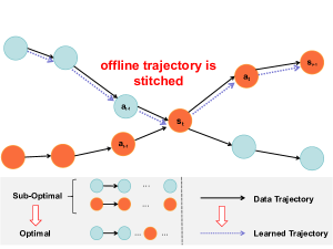
Figure 1: Offline stitching involves creating an optimal trajectory by stitching together sub-optimal trajectory fragments. In this figure, the learned purple path represents the optimal trajectory. ContextFormer demonstrates optimal performance in domains that necessitate stitching, as highlighted in Table 1. Demonstration of ContextFormer’s architecture is shown in Appendix B.1.

Task	QDT	DT	ContextFormer
sum	291.7	237.9	363.4

Table 1: Comparison among ContextFormer, Q-learning DT (QDT) (Yamagata et al., 2023), DT (Chen et al., 2021) on maze2d domains (Fu et al., 2020) (Averaged results in table 6.).

Depending on whether direct interaction with the online environment for acquiring new training samples, reinforcement learning (RL) can be categorized into offline RL (Kumar et al., 2020; Kostrikov et al., 2021) and online RL (Haarnoja et al., 2018; Schulman et al., 2017). Among that, offline RL aims to learn the optimal policy from a set of static trajectories collected by behavior policies without the need to interact with the online environment (Levine et al., 2020). One notable advantage of offline RL is its capacity to learn a more optimal behavior from a dataset consisting solely of sub-optimal trials (Levine et al., 2020). This feature renders it an efficient approach for applications where data acquisition is prohibitively expensive or poses potential risks, such as in the case of autonomous vehicles, and pipelines, etc.The success (obtain the optimal policy by learning on the sub-optimal trails) of these paradigms is attributed to its stitching capability (As illustrated in Figure 1, the stitching process involves exploiting and stitching candidate optimal trajectory fragments.) to fully leverage sub-optimal trails and seamlessly stitch them into an optimal trajectory, which has been discussed by (Fu et al., 2019, 2020; Hong et al., 2023)

Different from the majority of offline RL algorithms, Decision Transformer (DT) (Chen et al., 2021) abstracts the offline RL problems as sequence modeling process. Such paradigm achieved commendable performance across various offline benchmarks, including d4rl (Fu et al., 2021). Despite its success, recent studies suggest a limitation in DT concerning a crucial aspect of offline RL agents, namely, stitching (Yamagata et al., 2023). Specifically, DT appears to fall short in achieving the ability to construct an optimal policy by stitching together sub-optimal trajectories. Consequently, DT inherently lacks the capability to obtain the optimal policy through the stitching of sub-optimal trials. To address this limitation, investigating and enhancing the stitching capability of DT, or introducing additional stitching capabilities, holds the theoretical promise of further elevating its performance in offline tasks.

In order to endow the stitiching capability to transformer for decision making. QDT (Yamagata et al., 2023) proposed using Q-networks to relabel RTG, thereby endowing the stitching capability to DT. While experimental results suggest that relabeling the RTG through a pre-trained conservative Q network can enhance DT’s performance, this relabeling approach with a conservative critic tends to make the learned policy excessively conservative. Consequently, the policy’s ability to generalize is diminished. To further address this limitation, we approach it from the perspective of supervised and latent-based imitation learning (IL), $\textit{i}.\textit{e}.$ expert matching , and propose our method ContextFormer. In our approach, we employ the representations of a limited number of expert trajectories as demonstrations to stitch sub-optimal trajectories in latent space. This approach involves the joint and supervised training of a latent-conditioned transformer while optimizing contextual information. Stitching the sub-optimal trajectory from the perspective of expert matching serves as a remedy for the common issues present in both return conditioned DT and QDT. As shown in table 1 where ContextFormer achieves the best results on the tasks necessitating stitching capability.

Notably, our research is not confined to the offline RL setting. Rather, our study is centered around endowing the stitching capability to a transformer for decision-making. Importantly, there is currently no study demonstrating that a transformer can naturally stitch sub-optimal trajectory fragments without the assistance of RL. Thus, our approach can be considered as a novel and unique method to endow the stitching capability to transformer for decision-making within the realm of supervised learning. Furthermore, our approach has multiple advantages. Specifically, on the experimental aspect, our method can help to solve the limitation of a scalar reward function (information bottleneck (Vamplew et al., 2021)). On the theoretical aspect, our ContextFormer can be regarded as a novel approach to endow stitching capability to transformer from the perspective of expert matching. To validate the effectiveness of our approach, we primarily conducted comparisons and tests from two perspectives: 1) We compared ContextFormer with multiple competitive IL baselines under learning-from-observation (LfO) and learning-from-demonstration (LfD) settings. ContextFormer achieves competitive performance. 2) To demonstrate the advantages of ContextFormer over variants of DT, we compared the performance of ContextFormer with various DT variants on the same dataset, including return conditioned DT, Generalized DT (GDT) (Furuta et al., 2022), Prompt-DT(Xu et al., 2022), and PTDT-offline (Hu et al., 2023). Note that, despite our approach being an IL-based approach, our focus is on endowing the stitching capability to transformer for decision-making. Therefore, when conducting a comparison, we only focus on the DT variants’ performance on the same offline dataset, and the experimental results indicate that ContextFormer outperforms the aforementioned baselines. To summarize, our contributions can be outlined as follows:

• We imply expert matching as a complementary approach endowing stitching capability to transformer for decision making (we conduct mathematical derivation to support this claim), and correspondingly propose our algorithm ContextFormer.

• Extensive experimental results demonstrate ContextFormer can achieve competitive performance on multi-IL settings, and surpass multi-DT variants on the same offline datasets.

2 Related Work

Offline RL.

Offline RL learns policy from a static offline dataset and lacks the capability to interact with environment to collect new samples for training. Therefore, compared to online RL, offline RL is more susceptible to out-of-distribution (OOD) issues. Furthermore, OOD issues in offline RL have been extensively discussed. The majority competitive methods includes adding regularized terms to the objective function of offline RL to learn a conservative policy (Peng et al., 2019; Hong et al., 2023; Wu et al., 2022; Chen et al., 2022) or a conservative value network (Kumar et al., 2020; Kostrikov et al., 2021; An et al., 2021). By employing such methods, offline algorithms can effectively reduce the overestimation of OOD state actions. On the other hand, despite the existence of OOD issues in offline RL, its advantage lies in fully utilizing sub-optimal offline datasets to stitch offline trajectory fragments and obtain a better policy (Fu et al., 2019, 2021). This capability to improve the performance of policy by stitching sub-optimal trajectory fragments is known as policy improvement. However, previous researches indicate that DT lacks of stitching capabilities. Therefore, endowing stitching capabilities to DT could potentially enhance its sample efficiency in offline problem setting. In the context of offline DT, the baseline most relevant to our study is Q-learning DT (Yamagata et al., 2023) (QDT). Specifically, QDT proposes a method that utilizes a value network trained offline to relabel the RTG in the offline dataset, approximating the capability to stitch trajectories for DT. Unlike QDT, we endow stitching capabilities to DT from the perspective of expert matching.

IL.

Previous researches have extensively discussed various IL problem settings and mainly includes LfD(Argall et al., 2009; Judah et al., 2014; Ho & Ermon, 2016; Brown et al., 2020; Ravichandar et al., 2020; Boborzi et al., 2022), LfO (Ross et al., 2011; Liu et al., 2018; Torabi et al., 2019; Boborzi et al., 2022), offline IL (Chang et al., 2021; DeMoss et al., 2023; Zhang et al., 2023) and online IL (Ross et al., 2011; Brantley et al., 2020; Sasaki & Yamashina, 2021). The most related IL methods to our studies are Hindsight Information Matching (HIM) based methods (Furuta et al., 2022; Paster et al., 2022; Kang et al., 2023; Liu et al., 2023a; Gu et al., 2023), in particular, CEIL (Liu et al., 2023a) is the novel expert matching approach considering abstract various IL problem setting as a generalized and supervised HIM problem setting. Although both ContextFormer and CEIL share a commonality in calibrating the expert performance via expert matching, different from CEIL that our study focuses on endowing the stitching capabilities to transformer. Thus, the core objective of our study is distinct to offline IL that we don’t aim to enhance the IL domain but rather to endow stitching capability to transformer for decision making.

3 Preliminary

Before formally introducing our theory, we first introduce the basic concepts, which include RL, IL, HIM, and In-Context Learning (ICL).

RL.

We consider RL as a Markov Decision Processing (MDP) tuple,i.e.$\mathcal{M}=(\mathcal{S},\mathcal{A},\mathcal{R},T,r,\gamma,p(\mathbf{s}_{0}))$, where $\mathcal{S}$ denotes observation space, $\mathcal{A}$ denotes action space, and $T:\mathcal{S}\times\mathcal{A}\times\mathcal{S}\to\mathbb{R}^{+}$ is the transition (dynamics) probability, $r:\mathcal{S}\times\mathcal{A}\to\mathbb{R}$ is the reward function, $\gamma\in(0,1)$ is the discount factor, and $\mathbf{s}_{0}\sim p(\mathbf{s}_{0})$ is the initial observation, $p(\mathbf{s}_{0})$ is the initial state distribution. The goal of RL is to find the optimal policy $\pi^{*}(\cdot|\mathbf{s})$ to maximize the accumulated return $R(\tau)$, $\textit{i}.\textit{e}.$ $\pi^{*}\leftarrow\operatorname*{arg\,max}_{\pi}{\sum_{t=0}^{t=T}}_{(\mathbf{s}_{t},\mathbf{a}_{t})\sim\pi(\tau)}\gamma^{t}r(\mathbf{s}_{t},\mathbf{a}_{t})$, where $\tau=\{\mathbf{s}_{0},\mathbf{a}_{0},r(\mathbf{s}_{0},\mathbf{a}_{0}),\cdots,\mathbf{s}_{t},\mathbf{a}_{t},r(\mathbf{s}_{t},\mathbf{a}_{t})\}\sim\pi(\tau)$ is the rollout trajectory. In order to obtain the optimal policy, typically, we have to learn a Q network to estimate the expected return $R(\tau)=\sum_{t=0}^{t=T}\gamma^{t}r(\mathbf{s}_{t},\mathbf{a}_{t})$ for any given state action pairs $(\mathbf{s}_{t},\mathbf{a}_{t})\sim\tau_{\mathbf{z}}$,i.e.$Q(\mathbf{s}_{t},\mathbf{a}_{t})=\mathbb{E}[R(\tau)|\mathbf{s}=\mathbf{s}_{t},\mathbf{a}=\mathbf{a}_{t}]$, and optimize such Q network by Bellman backup: $\mathcal{J}(Q)={\mathrm{min}}\,{\mathbb{E}_{(\mathbf{s},\mathbf{a},r,\mathbf{s}^{\prime})\sim\tau}\big{[}Q(\mathbf{s},\mathbf{a})-\mathcal{T}_{\mathcal{M}}^{\pi}Q(\mathbf{s},\mathbf{a})\big{]}},$ where $\mathcal{T}_{\mathcal{M}}^{\pi}Q(\mathbf{s},\mathbf{a})=r(\mathbf{s},\mathbf{a})+\gamma Q(\mathbf{s}^{\prime},\pi(\cdot|\mathbf{s}^{\prime}))$. Correspondingly, update the policy $\pi$ by maximizing Q $\textit{i}.\textit{e}.$ $\mathcal{J}{(\pi)}={\mathrm{max}}_{\pi}\,Q(\pi(\cdot|\mathbf{s}),\mathbf{s})$ or actor critic (a2c) or etc. Different from the predominate offline RL approaches, DT abstracts offline RL as sequence modeling $\textit{i}.\textit{e}.$ $\mathbf{a}_{t}\leftarrow\pi(\cdot|\hat{R}_{0},\mathbf{s}_{0},\mathbf{a}_{0},\cdots,\hat{R}_{t},\mathbf{s}_{t})$, where $\hat{R}_{t^{\prime}}=\sum_{t=t^{\prime}}^{t=T}\gamma^{t-t^{\prime}}r(\mathbf{s}_{t},\mathbf{a}_{t})$ denotes Return-to-Go (RTG).

IL.

In the IL problem setting, the reward function $r(\mathbf{s}_{t},\mathbf{a}_{t})$ cannot be accessed, but the demonstrations $\mathcal{D}_{\rm demo}=\{\tau_{\rm demo}=\{\mathbf{s}_{0},\mathbf{a}_{0},\cdots,\mathbf{s}_{t},\mathbf{a}_{t}\}|\tau_{\rm demo}\sim\pi^{*}(\tau)\}$ or observations $\mathcal{D}_{\rm obs}=\{\ \tau_{\rm obs}=\{\mathbf{s}_{0},\cdots,\mathbf{s}_{t}\}|\tau_{\rm obs}\sim\pi^{*}(\tau)\}$ are available, where $\pi^{*}$ denotes the expert policy. Accordingly, the goal of IL is to recover the performance of expert policy by utilizing extensive sub-optimal trajectories $\hat{\tau}\sim\hat{\pi}(\tau)$ imitating expert demonstrations or observations, where $\hat{\pi}(\cdot|\tau)$ is the sub-optimal policy. Furthermore, according to the objective of imitation, it has two general settings: 1) In the setting of LfD, we imitate from demonstration. 2) In the setting of LfO, we imitate from observation.

Hindsight Information Matching (HIM).

Furuta et al. defined the HIM as training conditioned policy with hindsight information $\textit{i}.\textit{e}.$ learning a contextual policy $\pi(\cdot|\mathbf{z},\mathbf{s})$ by Equation 1.

$$\pi(\cdot|\mathbf{z},\mathbf{s})\leftarrow{\operatorname*{arg\,min}}_{\pi}\mathbb{E}_{\mathbf{z}\sim p(\mathbf{z}),\tau_{\mathbf{z}}\sim\pi_{\mathbf{z}}}[D(\mathbf{z},I_{\phi}(\tau_{\mathbf{z}}))],$$ (1)

where $I_{\phi}(\tau_{\mathbf{z}}):\mathcal{S}\oplus\mathcal{A}\rightarrow\mathcal{Z}$ denotes the statistical function that can extract representation (or HI from the offline trajectories $\tau$, $\textit{i}.\textit{e}.$ $\mathbf{z}_{\tau}=I_{\phi}{(\tau_{\mathbf{z}})}$ (when utilizing $\tau_{\mathbf{z}}$ to compute $\mathbf{z}_{\tau}$, we derive $\mathbf{z}$ from $\tau$) and $D$ denotes the metric used to estimate the divergence between the initialized latent representation $\forall\mathbf{z}\in\mathcal{Z},\mathbf{z}\sim p(\mathbf{z})$ and the trajectory HI $\textit{i}.\textit{e}.$ $I_{\phi}(\tau_{\mathbf{z}})$, $\oplus$ denotes concatenation. In particular, $\tau_{\mathbf{z}}$ will be optimal if we set $\mathbf{z}=\mathbf{z}^{*}$, we regard the expert trajectory as $\tau^{*}$ and it satisfy: $D(I_{\phi}(\tau^{*}),\mathbf{z}^{*})=0$, therefore, we can condition on $\mathbf{z}^{*}$ to rollout expert trajectory $\tau_{\mathbf{z}^{*}}$.

In-Context Learning (ICL).

Recent studies demonstrate that DT can be prompted with offline trajectory fragments to conduct fine-tuning and adaptation on new similar tasks (Xu et al., 2022). $\textit{i}.\textit{e}.$ $\mathbf{a}_{t}\leftarrow\pi(\cdot|\tau_{\rm prompt}\oplus\{\mathbf{s}_{0},\mathbf{a}_{0},\cdots,\mathbf{s}_{t}\})$, where the prompt is: $\tau_{\rm prompt}=\{\mathbf{s}_{0},\mathbf{a}_{0},\cdots,\mathbf{s}_{k},\mathbf{a}_{k}\}$. Despite that ContextFormer also utilizes the contextual information. However, it is different from DT that ContextFormer condition on the offline trajectory’s latent representation rather prompt to inference, which enables the long horizontal information being embedded into the contextual embedding, and such contextual embedding contains richer information than prompt-based algorithm, therefore, contextual embedding is possible to consider selecting useful samples with longer-term future information during the training process, making it more likely to assist in stitching sub-optimal trajectories.

4 Can expert matching endow stitching to transformer for decision making?

In this section, we conduct mathematical derivations and employ theoretical analysis to indicate how expert matching can endow aforementioned stitching capability to transformer for decision making. Although our mathematical derivations are in the realm of a tabular setting, our experimental results suggest that our approach can be extended to a continuous control setting. (We also provide an intuitive and concise explanation in Appendix D.) We first define the basic concepts we need. Specifically, we define latent conditioned sequence modeling as definition 4.1, expert matching based IL as definition 4.2.

definition 4.1 (latent conditioned sequence modeling).

Given the latent conditioned sequence model $\pi_{\mathbf{z}}(\cdot|\tau_{\mathbf{z}})$, the latent conditioned sequence modeling process can be formulated as $\mathbf{a}_{t}\leftarrow\pi_{\mathbf{z}}(\cdot|\mathbf{z},\mathbf{s}_{0},\mathbf{a}_{0},\cdots,\mathbf{z},\mathbf{s}_{t})$, where $D(\mathbf{z}||I_{\phi}(\tau))\leq\epsilon$, $D$ is divergence, the input of $\pi_{\mathbf{z}}$ is $\tau_{\mathbf{z}}=\{\mathbf{z},\mathbf{s}_{0},\mathbf{a}_{0},\cdots,\mathbf{z},\mathbf{s}_{t},\mathbf{a}_{t}\}$, where $\tau=\{\mathbf{s}_{0},\mathbf{a}_{0},\cdots,\mathbf{s}_{t},\mathbf{a}_{t}\}$, $t\in[0,T]$ and $\mathbf{z}\in\mathcal{Z}$, $\mathbf{z}\ll T\cdot\mathcal{S}$. (Additionally, we define $\pi_{I_{\phi}(\tau)}$ as $\pi_{\mathbf{z}}$ when conditioning on $I_{\phi}(\tau)$, this process is formulated as Equation 4)

Liu et al. advocates that optimizing a contextual objective to achieve expert matching, based on this exploration and the concept of latent conditioned sequence modeling (definition 4.1), we define the expert matching objective of sequence modeling in definition 4.2.

definition 4.2 (expert matching).

Given the HI extractor $I_{\phi}(\cdot|\tau)$, based on definition 4.1, the process of expert matching can be defined as: jointly optimizing the contextual information (or HI) $\mathbf{z}^{*}$ and contextual policy $\pi_{\mathbf{z}}(\cdot|\tau)$ to approach expert policy $\textit{i}.\textit{e}.$ $\pi_{\mathbf{z}^{*}}\leftarrow\operatorname*{arg\,min}_{\pi_{\mathbf{z}^{*}}}D(I_{\phi}(\tau^{*})||\mathbf{z}^{*})-D(I_{\phi}(\hat{\tau})||\mathbf{z}^{*})+D_{\rm KL}(\pi_{I_{\phi(\tau)}}(\cdot|\tau_{I_{\phi}(\tau)})||\pi^{*}(\cdot|\tau))$, where $\hat{\tau}\sim\hat{\pi}(\tau)$ denotes the sub-optimal trajectory, $\tau^{*}\sim\pi^{*}(\tau)$ denotes the optimal trajectory, and $\pi^{*}(\cdot|\tau)$ denotes the expert policy, and $\tau$ denotes $\tau^{*}$/$\hat{\tau}$ $\textit{i}.\textit{e}.$ $\tau\sim\pi^{*}(\tau)$ or $\hat{\pi}(\tau)$.

As mentioned in definition 4.2, the optimal contextual embedding $\mathbf{z}^{*}$ should have to be calibrated with the the expert trajectory’s HI and away from the sub-optimal trajectory’s HI :

$$\small\begin{split}\mathcal{J}_{\mathbf{z}^{*}}=\min_{\mathbf{z}^{*},I_{\phi}}\mathbb{E}_{\tau^{*}\sim\pi^{*}(\tau)}[||\mathbf{z}^{*}-I_{\phi}(\tau^{*})||]\\ -\mathbb{E}_{\hat{\tau}\sim\hat{\pi}}[||\mathbf{z}^{*}-I_{\phi}(\hat{\tau})||],\end{split}$$ (2)

based on the aforementioned intuitive objective and the conceptions of latent conditioned sequence modeling (definition 4.1), expert matching (definition 4.2). We begin by further driving the objective of contextual optimization in expert matching:

Theorem 4.3.

Given the optimal sequence model $\pi^{*}(\cdot|\tau)$, the sub-optimal sequence model $\hat{\pi}(\cdot|\tau)$, the HI extractor $I_{\phi}(\cdot|\tau)$, contextual embedding $\mathbf{z}^{*}$. Minimizing $\mathcal{J}_{I_{\phi},\mathbf{z}^{*}}=\mathbb{E}_{\tau^{*}\sim\pi^{*}(\tau)}[||\mathbf{z}^{*}-I_{\phi}(\cdot|\tau^{*})||]-\mathbb{E}_{\hat{\tau}\sim\hat{\pi}(\tau)}[||\mathbf{z}^{*}-I_{\phi}(\cdot|\hat{\tau})||]$ is equivalent to:

$$\small\begin{split}\min_{\mathbf{z}^{*},I_{\phi}}\int_{\tau\sim\mathcal{S}\oplus\mathcal{A}}\mathbb{I}(\pi^{*}(\tau)\geq\hat{\pi}(\tau))(\pi^{*}(\tau)-\hat{\pi}(\tau))||\mathbf{z}^{*}-I_{\phi}(\tau)||d\tau\\ +\int_{\tau\sim\mathcal{S}\oplus\mathcal{A}}\mathbb{I}(\pi^{*}(\tau)\leq\hat{\pi}(\tau))(\pi^{*}(\tau)-\hat{\pi}(\tau))||\mathbf{z}^{*}-I_{\phi}(\tau)||d\tau\end{split}$$

, where $\mathbb{I}$ denotes indicator.

Proof of Theorem 4.3 see Appendix A.4.

The result is formalized in Theorem 4.3, illustrating that optimizing Equation 2 serves as an approach to extract information from sub-optimal trajectories that aligns with expert trajectories for training $\mathbf{z}^{*}$. Simultaneously, it also serves as a filter for non-expert HI, ensuring that $\mathbf{z}^{*}$ diverges from such non-expert information as much as possible. Building on the analysis in Theorem 4.3, we further highlight the implication that Equation 2 can proficiently filter out non-expert information from sub-optimal trajectories. By leveraging expert information as complementary data for training $\mathbf{z}^{*}$, we thereby enhance the diversity of rolled out trajectories when conditioning on $\mathbf{z}^{*}$, as outlined in Proposition 4.4.

Proposition 4.4.

Continuing from Theorem 4.3, optimizing Equation 2 is tantamount to filtering out non-expert HI from sub-optimal trajectories.

Proof of Proposition 4.4, see Appendix A.5.

To begin with establishing the link between latent conditioned sequence modeling, expert matching, and contextual optimization, we initiate by modeling the disparity that arises when the sub-optimal policy $\hat{\pi}(\cdot|\tau)$ and optimal policy $\pi^{*}(\cdot|\tau)$ evaluate the same time steps simultaneously. This modeling is formally articulated in Theorem 4.5.

Theorem 4.5.

Given sequence model $\mathbf{a}_{t}\leftarrow\pi^{*}_{\theta^{*}}(\cdot|\tau_{t+k-1}\oplus\mathbf{s}_{t})$, which is L-smoothed $\textit{i}.\textit{e}.$ $||\pi^{*}_{\theta^{*}}(\cdot|\tau_{t+k-1}\oplus\mathbf{s}_{t})-\hat{\pi}_{\hat{\theta}}(\cdot|\tau_{t+k-1}\oplus\mathbf{s}_{t})||\leq L||\theta^{*}-\hat{\theta}||$, and given the optimal trajectory $\tau^{*}\sim\pi^{*}(\tau)$ and the sub-optimal trajectory $\hat{\tau}\sim\hat{\pi}(\tau)$. If we evaluate the contextual policy infinite times, then the performance difference between $\pi^{*}_{\theta^{*}}(\cdot|\tau^{*})$ and $\hat{\pi}_{\hat{\theta}}(\cdot|\hat{\tau})$ is:

$$\mathcal{L}(\pi^{*}_{\theta^{*}},\hat{\pi}_{\hat{\theta}})\geq 1-\mathbb{E}_{\hat{\tau}\sim\hat{\pi}}[||\pi^{*}_{\theta^{*}}(\hat{\mathbf{a}}_{t}|\hat{\tau}_{t:t+k-1}\oplus\hat{\mathbf{s}}_{t})||]$$

$$+L||\theta^{*}-\hat{\theta}||$$

Proof of Theorem 4.5 see Appendix A.6.

In Theorem 4.5, we illustrate that the disparity in performance between optimal and sub-optimal sequential models is associated with:

$$\begin{split}\max\mathbb{E}_{\hat{\tau}\sim\hat{\pi}(\tau)}[||\pi^{*}_{\theta^{*}}(\hat{\mathbf{a}}_{t}|\hat{\tau}_{t:t+k-1}\oplus\hat{\mathbf{s}}_{t})||]\end{split}$$ (3)

Observing from the mathematical expression of Equation 3, we observe that it inherently seeks to maximize the probability of trajectories generated by the sub-optimal policy being also sampled from the expert policy. This formulation aligns with our intuitive understanding that approaching the training policy to expert ones involves driving the training policy’s decisions to align entirely with the expert model. Consequently, we continue the derivation in Theorem 4.5 and Proposition 4.4 to demonstrate that joint optimization of Equations 2 and 4 increase $\mathbb{E}_{\hat{\tau}\sim\hat{\pi}(\tau)}[||\pi^{*}_{\theta^{*}}(\hat{\mathbf{a}}_{t}|\hat{\tau}_{t:t+k-1}\oplus\hat{\mathbf{s}}_{t})||]$, thereby minimizing $\mathcal{L}(\pi_{\mathbf{z}^{*}},\pi^{*})$ as presented in Theorem 4.3. Furthermore, Equations 2 and 4 also aid in stitching sub-optimal trajectories to approximate the expert policy, as formalized in Lemma 4.6.

Lemma 4.6.

Jointly optimizing the latent conditioned sequence policy defined as definition 4.1 and the objective of expert matching $\textit{i}.\textit{e}.$ definition 4.2 can help to stitch the sub-optimal trajectory fragments and to minimize the performance difference between the contextual policy $\pi_{\mathbf{z}^{*}}(\cdot|\tau_{\mathbf{z}^{*}})$ and optimal policy $\pi^{*}(\cdot|\tau)$.

Proof of Lemma 4.6 see Appendix A.7.

5 Context Transformer (ContextFormer)

We have mentioned the limitations of previous DT variants in In the section of introduction: 1) DT methods lack the stitching capability that is the crucial factor for policy improvement. 2) these methods are imitated by the information bottleneck because of the scalar Return condition. 3) Despite QDT stitches the sub-optimal trajectories by relabeling the sub-optimal dataset with conservative Q network, the conservative critic may diminish the exploratory of DT. In order to address these limitations, we propose ContextFormer which is based on expert matching and utilizing the representation of expert trajectories to stitch sub-optimal trajectory fragments, training transformer with supervised objective, thereby approaching expert policy, while getting rid of the limitations of conservative offline objective.

Algorithm 1  ContextFormer

Require: HI extractor $I_{\phi}(\cdot|\tau)$, Contextual policy $\pi_{\mathbf{z}}(\cdot|\tau)$, sub-optimal offline datasets $D_{\hat{\tau}}\sim\hat{\pi}$, randomly initialized contextual embedding $\mathbf{z}^{*}$, and demonstrations (expert trajectories) $D_{\rm\tau^{*}}\sim\pi^{*}$   Training:

1:  Sample sub-optimal trajectory $\hat{\tau}$ from $\mathcal{D}_{\hat{\tau}}$, and sampling batch expert trajectory $\tau^{*}$ from $D_{\rm\tau^{*}}$.

2:  update $I_{\phi}$ by Equation 4 and Equation 5 and VQ-loss (Appendix B, Equation 21). Update $\mathbf{z}^{*}$ by Equation 5.

3:  update $\pi_{\mathbf{z}}$ by Equation 4.

Evaluation:

1:  Initialize $t=0$; $\mathbf{s}_{t}\leftarrow\rm env.reset()$; $\tau_{\mathbf{z}^{*}}=\{\mathbf{z}^{*},\mathbf{s}_{0}\}$; ${\rm done}=\rm False$, $R=0$, $N=0$.

2:  while $t\leq N$ or not done do

3:    $\mathbf{a}_{t}\leftarrow\pi_{\mathbf{z}*}(\cdot|\tau_{\mathbf{z}^{*}})$;

4:    $\mathbf{s}_{t+1},{\rm done},r_{t}\leftarrow\rm env.step(\mathbf{a}_{t})$;

5:    $\tau_{\mathbf{z}^{*}}.{\rm append}(\mathbf{a}_{t},\mathbf{z}^{*},\mathbf{s}_{t+1})$; t+=1

6:    $R+=r_{t}$

7:  end while

8:  Return $R$

5.1 Method

Training Procedure.

Given the HI extractor $I_{\phi}$ (in our Practical implementation we utilize BERT (Devlin et al., 2019) as HI extractor), contextual embedding $\mathbf{z}^{*}$ and contextual policy (in our Practical implementation we utilize DT (Chen et al., 2021) model as our backbone) $\pi_{\mathbf{z}}(\cdot|\tau_{t-k:t})$, where $\tau_{t-k:t}=\{\mathbf{s}_{t-k},\mathbf{a}_{t-k}\cdots,\mathbf{s}_{t},\mathbf{a}_{t}\}$ means the sampled trajectory with window size $k$. We model the contextual sequence model by the aforementioned latent conditioned sequence modeling defined in definition 4.1, training the contextual sequence model with the expert matching objective defined in definition 4.2 and, we optimize the contextual policy by optimizing Equation 4:

$$\small\begin{split}\mathcal{J}_{\pi_{\mathbf{z}},I_{\phi}}=\mathbb{E}_{\tau\sim(\pi^{*},\hat{\pi})}[||\pi_{\mathbf{z}}(\cdot|I_{\phi}(\tau),\mathbf{s}_{0},\mathbf{a}_{0},\cdots,I_{\phi}(\tau),\mathbf{s}_{t})\\ -\mathbf{a}_{t}||],\end{split}$$ (4)

where $\tau=\big{\{}\mathbf{s}_{0},\mathbf{a}_{0},\cdots,\mathbf{s}_{t},\mathbf{a}_{t}\big{\}}$ is the rollout trajectory, while $\hat{\pi}$ and $\pi^{*}$ are separated to the sub-optimal and optimal policies. Meanwhile, we also optimize the HI extractor $I_{\phi}$ and contextual embedding $\mathbf{z}^{*}$ via Equations 4 and 5:

$$\small\begin{split}\mathcal{J}_{\mathbf{z}^{*},I_{\phi}}=\min\limits_{\mathbf{z}^{*},I_{\phi}}\mathbb{E}_{\hat{\tau}\sim\hat{\pi}(\tau),\tau^{*}\sim\pi^{*}(\tau)}[||\mathbf{z}^{*}-I_{\phi}(\tau^{*})||\\ -||\mathbf{z}^{*}-I_{\phi}(\hat{\tau})||]\end{split}$$ (5)

Evaluation Procedure.

Based on the modeling approach defined in definition 4.1, we utilize the contextual embedding $\mathbf{z}^{*}$ learned through Equation 6 as the goal for each inference moment of our latent conditioned sequence model, thereby auto-regressively rolling out trajectory in the environment to complete the testing. The evaluation process has been detailed in Algorithm 1.

Table 2: Normalized scores (averaged over 10 trails for each task) when we vary the number of the expert demonstrations (#5, #10, and #20). Scores within two points of the maximum score are highlighted.

Offline IL settings		Hopper-v2			Halfcheetah-v2			Walker2d-v2			Ant-v2			sum
		m	mr	me	m	mr	me	m	mr	me	m	mr	me
LfD #5	ORIL (TD3+BC)	42.1	26.7	51.2	45.1	2.7	79.6	44.1	22.9	38.3	25.6	24.5	6.0	408.8
	SQIL (TD3+BC)	45.2	27.4	5.9	14.5	15.7	11.8	12.2	7.2	13.6	20.6	23.6	-5.7	192.0
	IQ-Learn	17.2	15.4	21.7	6.4	4.8	6.2	13.1	10.6	5.1	22.8	27.2	18.7	169.2
	ValueDICE	59.8	80.1	72.6	2.0	0.9	1.2	2.8	0.0	7.4	27.3	32.7	30.2	316.9
	DemoDICE	50.2	26.5	63.7	41.9	38.7	59.5	66.3	38.8	101.6	82.8	68.8	112.4	751.2
	SMODICE	54.1	34.9	64.7	42.6	38.4	63.8	62.2	40.6	55.4	86.0	69.7	112.4	724.7
	CEIL	94.5	45.1	80.8	45.1	43.3	33.9	103.1	81.1	99.4	99.8	101.4	85.0	912.5
	ContextFormer	74.9	77.8	103.0	43.1	39.6	46.6	80.9	78.6	102.7	103.1	91.5	123.8	965.6
LfD #10	ORIL (TD3+BC)	42.0	21.6	53.4	45.0	2.1	82.1	44.1	27.4	80.4	47.3	24.0	44.9	514.1
	SQIL (TD3+BC)	50.0	34.2	7.4	8.8	10.9	8.2	20.0	15.2	9.7	35.3	36.2	11.9	247.6
	IQ-Learn	11.3	18.6	20.1	4.1	6.5	6.6	18.3	12.8	12.2	30.7	53.9	23.7	218.7
	ValueDICE	56.0	64.1	54.2	-0.2	2.6	2.4	4.7	4.0	0.9	31.4	72.3	49.5	341.8
	DemoDICE	53.6	25.8	64.9	42.1	36.9	60.6	64.7	36.1	100.2	87.4	67.1	114.3	753.5
	SMODICE	55.6	30.3	66.6	42.6	38.0	66.0	64.5	44.6	53.8	86.9	69.5	113.4	731.8
	CEIL	113.2	53.0	96.3	64.0	43.6	44.0	120.4	82.3	104.2	119.3	70.0	90.1	1000.4
	ContextFormer	75.4	76.2	102.1	42.8	39.1	44.6	81.2	78.8	99.9	102.7	90.6	122.2	955.6
LfO #20	ORIL (TD3+BC)	55.5	18.2	55.5	40.6	2.9	73.0	26.9	19.4	22.7	11.2	21.3	10.8	358.0
	SMODICE	53.7	18.3	64.2	42.6	38.0	63.0	68.9	37.5	60.7	87.5	75.1	115.0	724.4
	CEIL	44.7	44.2	48.2	42.4	36.5	46.9	76.2	31.7	77.0	95.9	71.0	112.7	727.3
	ContextFormer	67.9	77.4	97.1	43.1	38.8	55.4	79.8	79.9	109.4	102.4	86.7	132.2	970.1

5.2 Practical Implementation of ContextFormer

Our approach is summarized in Algorithm 1. Specifically, when optimizing $I_{\phi}$, we selected the BERT model as the HI extractor $I_{\phi}$. The optimization of $I_{\phi}$ involves a joint utilization of: 1) Vector Quantization Variational Autoencoder (VQ-VAE) (van den Oord et al., 2018) loss (Appendix B, Equation 21), and 2) latent conditioned supervised training loss (Equation 4). Concerning the VQ-VAE training objective, we employ $I_{\phi}$ as the encoder and a multi-layer perceptron (MLP) as the decoder to construct the VQ-VAE. We input the trajectory (includes expert and sub-optimal) to BERT to extract trajectory representations (latent or contextual information) and then use an MLP-based retroactive inference approach to reconstruct the input trajectory, calculating the VQ-VAE loss to optimize $I_{\phi}$. For detailed information on our specific deployment scheme, please refer to (Appendix B). On the other hand, when optimizing $\pi_{\mathbf{z}}(\cdot|\tau)$, we directly employ a supervised training objective to optimize $\pi_{\mathbf{z}}$, i.e., using Equation 4. In the following section, we conduct experiments to validate the effectiveness of ContextFormer. On one hand, we verify ContextFormer’s capability to leverage the expert dataset to aid in learning from sub-optimal datasets (section 6.4). On the other hand, we compare the performance difference between ContextFormer and DT variants in section 6.5.

6 Evaluation

Our approach utilizes expert matching to endow stitching to transformer for decision making. We validate ContextFormer from two majority aspects. On the on hand, we validate the capability that utilizing expert trajectory to assist in learning on sub-optimal trajectories by testing on IL tasks. On the other hand, we compare ContextFormer and multiple DT variants on the same datasets.

6.1 Experimental settings

IL.

In the majority of our IL experiments, we utilize 5 to 20 expert trajectories and conduct evaluations under various settings, including both LfO and LfD settings. The objective of these tasks is to emulate $\pi^{*}(\cdot|\tau)$ by leveraging a substantial amount of sub-optimal offline dataset $\hat{\tau}\sim\hat{\pi}(\tau)$, aiming to achieve performance that equals or even surpasses that of the expert policy $\pi^{*}(\cdot|\tau)$. In particular, when conduct LfO setting, we imitate from $\tau_{\rm obs}$, when conduct LfD setting we imitate from $\tau_{\rm demo}$ (both $\tau_{\rm demo}$ and $\tau_{\rm obs}$ are mentioned in section Preliminary). And we utilize $\tau_{\rm demo}$/$\tau_{\rm obs}$ as $\tau^{*}$ (contextual optimization) in LfD/LfO setting to optimize $\mathbf{z}^{*}$ by Equation 5 and Equation 4. We optimize $\pi_{\mathbf{z}}(\cdot|\tau_{\mathbf{z}})$ by Equation 4 (policy optimization).

DT comparisons.

Note that, we are disregarding variations in experimental settings such as IL, RL, etc. Our focus is on controlling factors (data composition, model architecture, etc.), with a specific emphasis on comparing model performance. In particular, ContextFormer is trained under the same settings as IL, while DT variants underwent evaluation using the original settings.

6.2 Training datasets

IL.

Our experiments are conducted on four Gym-Mujoco (Brockman et al., 2016) environments, including Hopper-v2, Walker2d-v2, Ant-v2, and HalfCheetah-v2. These tasks are constructed utilizing D4RL (Fu et al., 2021) datasets including medium-replay (mr), medium (m), medium-expert (me), and expert (exp).

DT comparisons.

When comparing ContextFormer with DT, GDT, and Prompt-DT, we utilize the datasets discussed in IL. Additionally, we compare QDT and ContextFormer on the maze2d domain, specifically designed to assess their stitching abilities (Yamagata et al., 2023). In terms of the dataset we utilize for training baselines, we ensure consistency in our comparisons by using identical datasets. For instance, when comparing ContextFormer (LfD #5) on Ant-medium, we train DT variants with the same datasets (5 expert trajectories and the entire medium dataset).

6.3 Baselines

IL. Our IL baselines include ORIL (Zolna et al., 2020), SQIL (Reddy et al., 2019), IQ-Learn (Garg et al., 2022), ValueDICE (Kostrikov et al., 2019), DemoDICE (Kim et al., 2022), SMODICE (Ma et al., 2022), and CEIL (Liu et al., 2023a). The results of these baselines are directly referenced from Liu et al., which are utilized to be compared with ContextFormer in both the LfO and LfD settings, intuitively showcasing the transformer’s capability to better leverage sub-optimal trajectories with the assistance of expert trajectories (hindsight information).

DT comparisons. To further substantiate our theoretical claims (Theorem 4.5 and Lemma 4.6), we carry out comparisons between ContextFormer and DT, DT variants (Prompt-DT, PTDT-offline, and QDT), utilizing the same dataset. This involves comparing the training performance of various transformers.

6.4 Comparison with multiple IL baselines

We conduct various IL task settings including LfO and LfD to assess the performance of ContextFormer. As illustrated in table 2, ContextFormer outperforms selected baselines, achieving the highest performance in LfD #5 and LfO #20, showcasing respective improvements of 5.8% and 33.4% compared to the best baselines (CEIL). Additionally, ContextFormer closely approach CEIL under the LfO #20 setting. These results demonstrate the effectiveness of our approach in utilizing expert information to assist in learning the sub-optimal policy, which is cooperated with our analysis (Theorem 4.5 and Lemma 4.6). However, the core of our study is to indicate that our method can endow stitching capability to transformer for policy improvement, therefore, we also have to compare ContextFormer with DT and efficient DT variants to further valid our claim.

6.5 Comparison with various DT variants

ContextFormer vs. Return Conditioned DT.

ContextFormer leverages contextual information as condition, getting riding of limitations such as the information bottleneck associated with scalar return. Additionally, we highlighted that expert matching aids the transformer in stitching sub-optimal trajectories. Consequently, the performance of ContextFormer is expected to surpass that of DT when using the same training dataset. To conduct this comparison, we tested DT and ContextFormer on medium-replay, medium, and medium-expert offline RL datasets. Notably, we ensured consistency in the quality of training datasets between ContextFormer and DT variants by adding an equal or larger number of expert trajectories. As shown in table 3, ContextFormer (LfD #5) demonstrated approximately a 4.4% improvement compared to DT+5 expert trajectories (exp traj) and a 1.7% improvement compared to DT+10 exp traj.

ContextFormer vs. GDT.

Furuta et al. proposed utilizing HI to accelerate offline RL training and introduced GDT. However, it is essential to distinguish between ContextFormer and GDT. The key distinction lies in that ContextFormer conditions on long-horizon and task-level trajectory representations (rather local representations). This enables ContextFormer to consider global information and extract efficient examples from sub-optimal datasets, making it more likely to stitch sub-optimal fragments and approach the expert policy (Because an optimal decision requires considering global information, conditions that incorporate more information from future moments are more conducive to making better decisions.). We conduct a performance comparison between ContextFormer (LfD #5) and GDT using the same offline datasets. As shown in Table 5, our ContextFormer achieves the best performance across various GDT settings, including GDT+5 demonstration (demo) and GDT+5 best expert (best  traj) trajectories. Notably, ContextFormer demonstrates a remarkable 25.7% improvement compared to the best GDT (experimental results are shown in table LABEL:vsgdt).

Table 3: Comparison of performance between DT and ContextFormer (LfD #5).

Dataset	Task	DT+5 exp traj	DT+10 exp traj	ContextFormer (LfD #5)
Medium	hopper	69.5$\pm$ 2.3	72.0$\pm$ 2.6	74.9$\pm$ 9.5
	walker2d	75.0$\pm$ 0.7	75.7$\pm$ 0.4	80.9$\pm$ 1.3
	halfcheetah	42.5$\pm$ 0.1	42.6$\pm$ 0.1	43.1$\pm$ 0.2
medium-replay	hopper	78.9$\pm$ 4.7	82.2$\pm$ 0.5	77.8$\pm$ 13.3
	walker2d	74.9$\pm$ 0.3	78.3$\pm$ 5.6	78.6$\pm$ 4.0
	halfcheetah	37.3$\pm$ 0.4	37.6$\pm$ 0.8	39.6$\pm$ 0.4
sum		378.1	388.4	394.9

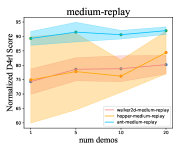
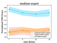
Figure 2: The model performance varies with the number of demonstrations. In this graph, we gradually increase the descriptions of expert trajectories and further observe the performance of ContextFormer in the LfD setting. We find that as the number of demonstrations increases, the performance of ContextFormer gradually improves.

Table 4: Comparison of performance between GDT (multiple settings) and ContextFormer (LfD #5). Specifically, we Compare the ContextFormer and GDT with 5 expert and GDT with 5 best trajectories, ContextFormer performs the best.

Task	Offline IL settings	GDT+5 demo	GDT+5 best  traj	ContextFormer (LfD #5)
hopper	medium	44.2$\pm$ 0.9	55.8$\pm$ 7.7	74.9$\pm$ 9.5
	medium-replay	25.6$\pm$ 4.2	18.3$\pm$ 12.9	77.8$\pm$ 13.3
	medium-expert	43.5$\pm$ 1.3	89.5$\pm$ 14.3	103.0$\pm$ 2.5
walker2d	medium	56.9$\pm$ 22.6	58.4$\pm$ 7.3	80.9$\pm$ 1.3
	medium-replay	19.4$\pm$ 11.6	21.3$\pm$ 12.3	78.6$\pm$ 4.0
	medium-expert	83.4$\pm$ 34.1	104.8$\pm$ 3.4	102.7$\pm$ 4.5
halfcheetah	medium	43.1$\pm$ 0.1	42.5$\pm$ 0.2	43.1$\pm$ 0.2
	medium-replay	39.6$\pm$ 0.4	37.0$\pm$ 0.6	39.6$\pm$ 0.4
	medium-expert	43.5$\pm$ 1.3	86.5$\pm$ 1.1	46.6$\pm$ 3.7
sum		399.2	514.1	644.9

Table 5: Comparison of performance between Prompt-DT, PTDT-offline and ContextFormer (LfD #1), ContextFormer performs the best. Notably, the experimental results of Prompt-DT and PTDT-offline are directly quated from (Hu et al., 2023).

Dataset	Task	Prompt-DT	PTDT-offline	ContextFormer (LfD #1)
medium	hopper	68.9$\pm$ 0.6	71.1$\pm$ 1.7	67.8$\pm$ 6.7
	walker2d	74.0$\pm$ 1.4	74.6$\pm$ 2.7	80.7$\pm$ 1.6
	halfcheetah	42.5$\pm$ 0.0	42.7$\pm$ 0.1	43.0$\pm$ 0.2
sum		185.4	188.4	191.5

ContextFormer vs Prompt-DT.

Prompt learning is an extensively discussed paradigm in natural language processing (NLP) (Liu et al., 2021). A shared characteristic between Prompt-DT and ContextFormer is the utilization of contextual information. However, the significant differences in contextual information between prompt learning and contextual information is that prompts can only provide a limited number of examples. In contrast, ContextFormer’s contextual embedding integrates all information from expert trajectories, encompassing all the details of expert trajectories. To validate those analysis, we compare ContextFormer (LfD #1) with Prompt-DT and PTDT-offline. The experimental results demonstrate that ContextFormer outperforms PTDT-offline by 1.6$\%$, Prompt-DT by 3.3$\%$ (in table 5).

ContextFormer vs. QDT.

The final baseline we selected for comparison is QDT. QDT highlights the lack of stitching capabilities in DT and addresses this limitation by utilizing a pre-trained conservative Q network to relabel the offline dataset, thereby providing DT with stitching capabilities. Our approach differs from QDT in that we leverage representations of expert trajectories to stitch sub-optimal trajectories, enabling achieving better performance than behavioral policy. The advantages of ContextFormer line in two aspects. On one hand, our method can overcome the information bottleneck associated with scalar reward. On the other hand, our method adopts a supervised learning approach, thereby eliminating the constraints of a conservative policy. Moreover, as demonstrated in table 6, we evaluate ContextFormer on multiple tasks in the maze2d domain, utilizing the top 10 trials ranked by return as demonstrations. Our algorithm achieves a score of 364.3, surpassing all DTs.

Table 6: Comparison of the performance difference between QDT and ContextFormer (LfD #10). ContextFormer (LfD #10) performs the best. Notably, the experimental results of QDT, DT and CQL are directly quated from (Yamagata et al., 2023).

Task	QDT	DT	CQL	ContextFormer (LfD #top 10 $\tau$)
maze2d-open-v0	190.1$\pm$37.8	196.4$\pm$39.6	216.7$\pm$ 80.7	204.2$\pm$13.3
maze2d-medium-v1	13.3$\pm$5.6	8.2$\pm$ 4.4	41.8$\pm$ 13.6	63.6$\pm$25.6
maze2d-large-v1	31.0$\pm$19.8	2.3$\pm$0.9	49.6$\pm$8.4	33.8$\pm$12.9
maze2d-umaze-v1	57.3$\pm$8.2	31.0$\pm$21.3	94.7$\pm$23.1	61.8$\pm$0.1
sum	291.7	237.9	402.8	363.4

7 Ablations

We vary the number of $\tau_{\rm demo}$ and testing its performance in the LfD setting. As illustrated in Figure 2, ContextFormer’s performance on medium-replay tasks generally improves with an increasing number of demonstrations. However, for medium and medium-expert datasets, there is only a partial improvement trend with an increasing number of $\tau_{\rm demo}$. In some medium-expert tasks, there is even a decreasing trend. This can be attributed to the presence of extensive diverse trajectory fragments in medium-replay, enabling ContextFormer to effectively utilize expert information for stitching sub-optimal trajectory fragments, resulting in improved performance on medium-replay tasks. However, in medium and medium-expert tasks, the included trajectory fragments may not be diverse enough, and expert trajectories in the medium-expert dataset might not be conducive to effective learning. As a result, ContextFormer exhibits less improvement on medium datasets and even a decrease in performance on medium-expert tasks.

8 Conclusions

We empower the transformer with stitching capabilities for decision-making by leveraging expert matching and latent conditioned sequence modeling. Our approach achieves competitive performance on IL tasks, surpassing all selected DT variants on the same dataset, thus demonstrating its feasibility. Furthermore, from a theoretical standpoint, we provide mathematical derivations illustrating that stitching sub-optimal trajectory fragments in the latent space enables the transformer to infer necessary decision-making aspects that might be missing in sub-optimal trajectories.

Ethical Claim and Social Impact

Transformer has revolutionized various domains, including sequential decision-making. However, previous studies have highlighted the absence of typical stitching capabilities in classical offline RL algorithms for transformers. Therefore, endowing the stitching capability to transformers is crucial to enhancing their ability to leverage sub-optimal trajectories for policy improvement.

In this research, we propose the incorporation of expert matching to empower transformers with the capacity to stitch sub-optimal trajectory fragments. This extension of stitching capability to transformers within the realm of supervised learning removes constraints related to scalar return. We believe that our approach enhances transformers by endowing them with stitching capability through expert matching, thereby contributing to improved sequential decision-making.

Appendix A Mathematics Proof.

In the main context, we have provided the Theorems 4.3 and 4.5, proposition 4.4 and Lemma 4.6 we utilized. Subsequently, in the following sections, we first give our assumptions, the in-equations we utilized, finally we will provide the mathematical proof of our Theorems and Lemma:

A.1 Symbol definitions

• $\pi^{*}(\cdot|\tau):$ optimal policy; $\hat{\pi}(\cdot|\tau):$ sub optimal policy; $\pi_{\mathbf{z}}(\cdot|\tau)$ contextual policy

• $\tau^{*}:$ optimal trajectory $\tau^{*}\sim\pi^{*}_{\theta^{*}}$; $\hat{\tau}:$ sub optimal trajectory $\hat{\tau}\sim\hat{\pi}_{\hat{\theta}}$.

• $P^{\theta}(\tau)$: Sample probability, it is utilized to estimate the probability of $\tau$ be sampled from policy $\pi^{*}_{\theta^{*}}$.

• $\oplus$ means concatenation utilized to represent the fragment concatenation process, $\textit{i}.\textit{e}.$ $\{\mathbf{s}_{0},\mathbf{a}_{0},\cdots,\mathbf{s}_{t}\}\oplus\mathbf{a}_{t}=\{\mathbf{s}_{0},\mathbf{a}_{0},\cdots,\mathbf{s}_{t},\mathbf{a}_{t}\}$

A.2 Assumptions

Assumption A.1.

There is a constant L such that for any $\mathbf{a}_{t+k}$, $\tau_{t:t+k}$, the None Markov Decision Process (Non-MDP) policy $\pi_{\theta}(\mathbf{a}_{t+k}|\tau^{*}_{t:t+k-1}\oplus\mathbf{s}_{t})$ is L-smooth regarding $\bigg{|}\bigg{|}\pi_{\theta_{1}}(\mathbf{a}_{t}|\tau^{*}_{t:t+k-1}\oplus\mathbf{s}_{t})-\pi_{\theta_{2}}(\mathbf{a}_{t}|\tau^{*}_{t:t+k-1}\oplus\mathbf{s}_{t})\bigg{|}\bigg{|}\leq L\bigg{|}\bigg{|}\theta_{1}-\theta_{2}\bigg{|}\bigg{|}$, $\forall\theta_{1}$ and $\theta_{2}$.

A.3 In-equality we utilized

• In-equality 1: Based on Assumption A.1, we have can immediately obtain the common In-equality: $\bigg{|}\bigg{|}\pi_{\theta_{1}}(\mathbf{a}_{t}|\tau^{*}_{t:t+k-1}\oplus\mathbf{s}_{t})-\pi_{\theta_{2}}(\mathbf{a}_{t}|\tau^{*}_{t:t+k-1}\oplus\mathbf{s}_{t})\bigg{|}\bigg{|}\leq L\bigg{|}\bigg{|}\theta_{1}-\theta_{2}\bigg{|}\bigg{|}$, $\forall\theta_{1}$ and $\theta_{2}$.

• In-equality 2: We also utilize multiple in-equations, including $|a|-|b|\leq||a\pm b||\leq|a|+|b|$

• In-equality 3: Minkowski in-equality, $[\mathbb{E}[|X+Y|^{p}]]^{\frac{1}{p}}\leq\mathbb{E}[|X|^{p}]^{\frac{1}{p}}+\mathbb{E}[|Y|^{p}]^{\frac{1}{p}}$, s.t. $0\leq p\leq\infty$.

• In-equality 4: Assume $P^{\theta^{*}}(\tau)$ is the sampling probability of $\tau$ when roll out the policy $\pi^{*}_{\theta^{*}}$. Subsequently, given another trajectory $\hat{\tau}$ that roll out by a different policy $\hat{\pi}_{\hat{\theta}}$, the sampling probability of $\hat{\tau}$ is lower than $\tau$, $\textit{i}.\textit{e}.$ $P^{\theta^{*}}(\tau^{*})\leq P^{\theta^{*}}(\hat{\tau})$

A.4 Proof of Theorem 4.3

Given our contextual optimization objective:

$$\begin{split}\mathcal{J}_{I_{\phi},\mathbf{z}^{*}}&=\min_{\mathbf{z}^{*},I_{\phi}}\mathbb{E}_{\hat{\tau}\sim\hat{\pi}_{\mathbf{z}^{*}},\tau^{*}\sim\pi^{*}}\Bigg{[}\bigg{|}\bigg{|}\mathbf{z}^{*}-I_{\phi}(\tau^{*})\bigg{|}\bigg{|}-\bigg{|}\bigg{|}\mathbf{z}^{*}-I_{\phi}(\hat{\tau})\bigg{|}\bigg{|}\Bigg{]}\end{split}$$ (6)

we regard $\pi^{*}(\tau)$ or $\hat{\pi}(\tau)$ as density function, separately estimating the probability of $\tau$ being sampled from policies $\pi^{*}(\cdot|\tau)$ and $\hat{\pi}(\cdot|\tau)$.

Then we first introduce importance sampling $\textit{i}.\textit{e}.$ $\int_{\tau^{*}\sim\pi^{*}(\tau)}f(\tau^{*})d\tau^{*}=\int_{\hat{\tau}\sim\hat{\pi}}\frac{\pi^{*}(\tau)}{\hat{\pi}(\tau)}f(\hat{\tau})d\hat{\tau}$.

And, we introduce: the transformation of sampling process from local domain to global domain $\textit{i}.\textit{e}.$ $\int_{\tau^{*}\sim\pi^{*}}f(\tau^{*})=\int_{\tau\sim\mathcal{S}\oplus\mathcal{A}}\pi^{*}(\tau)\cdot f(\tau)d\tau$, where $f(\tau)$ denotes the objective function.

we derivative:

$$\begin{split}\mathcal{J}_{I_{\phi},\mathbf{z}^{*}}&=\min_{\mathbf{z}^{*},I_{\phi}}\mathbb{E}_{\tau^{*}\sim\pi^{*}(\tau)}[||\mathbf{z}^{*}-I_{\phi}(\tau^{*})||]-\mathbb{E}_{\hat{\tau}\sim\hat{\pi}(\tau)}[||\mathbf{z}^{*}-I_{\phi}(\hat{\tau})||]\\ &=\min_{\mathbf{z}^{*},I_{\phi}}\mathbb{E}_{\hat{\tau}\sim\hat{\pi}(\tau)}[\frac{\pi^{*}(\tau)}{\hat{\pi}(\tau)}||\mathbf{z}^{*}-I_{\phi}(\hat{\tau})||]-\mathbb{E}_{\hat{\tau}\sim\hat{\pi}(\tau)}[||\mathbf{z}^{*}-I_{\phi}(\hat{\tau})||]\\ &=\min_{\mathbf{z}^{*},I_{\phi}}\mathbb{E}_{\hat{\tau}\sim\hat{\pi}(\tau)}[(\frac{\pi^{*}(\tau)}{\hat{\pi}(\tau)}-1)||\mathbf{z}^{*}-I_{\phi}(\hat{\tau})||]\\ &=\min_{\mathbf{z}^{*},I_{\phi}}\int_{\tau\sim\mathcal{S}\oplus\mathcal{A}}\hat{\pi}(\tau)\bigg{(}\frac{\pi^{*}(\tau)}{\hat{\pi}(\tau)}-1\bigg{)}||\mathbf{z}^{*}-I_{\phi}(\tau)||d\tau\\ &=\min_{\mathbf{z}^{*},I_{\phi}}\int_{\tau\sim\mathcal{S}\oplus\mathcal{A}}\bigg{(}\pi^{*}(\tau)-\hat{\pi}(\tau)\bigg{)}||\mathbf{z}^{*}-I_{\phi}(\tau)||d\tau\\ &=\min_{\mathbf{z}^{*},I_{\phi}}\underbrace{\int_{\tau\sim\mathcal{S}\oplus\mathcal{A}}\mathbb{I}(\pi^{*}\geq\hat{\pi})\bigg{(}\pi^{*}(\tau)-\hat{\pi}(\tau)\bigg{)}||\mathbf{z}^{*}-I_{\phi}(\tau)||d\tau}_{\rm term1}\\ &+\underbrace{\int_{\tau\sim\mathcal{S}\oplus\mathcal{A}}\mathbb{I}(\pi^{*}(\tau)\leq\hat{\pi}(\tau))\bigg{(}\pi^{*}(\tau)-\hat{\pi}(\tau)\bigg{)}||\mathbf{z}^{*}-I_{\phi}(\tau)||d\tau}_{\rm term2}\end{split}$$ (7)

where $\mathbb{I}$ means the indicator.

A.5 Proof of Equation 4.4.

Building upon Theorem 7, we can deduce that when the sampled trajectory ($\tau\sim\mathcal{S}\oplus\mathcal{A}$) is more likely to be sampled from $\pi^{*}(\tau)$ rather than $\hat{\pi}(\tau)$, optimizing $\min\mathcal{J}_{I_{\phi},\mathbf{z}^{*}}$ is tantamount to minimizing $\rm term1$ with respect to these trajectories identified by $\mathbb{I}(\pi^{*}(\tau)\leq\hat{\pi}(\tau))$ as expert HI, and minimizing $\rm term2$ with respect to trajectories identified by $\mathbb{I}(\pi^{*}(\tau)\geq\hat{\pi}(\tau))$ as non-expert information. This derivation results in $\mathbf{z}^{*}$ extracting HI that approaches $\tau^{*}$ from diverse datasets. Proof of term1. Given that $\mathbb{I}(\pi^{*}(\tau)\geq\hat{\pi}(\tau))$ we can derive that $\pi^{*}(\tau)-\hat{\pi}(\tau)\geq 0$, minimizing $\rm term1$ is consequently synonymous with minimizing $||\mathbf{z}^{*}-I_{\phi}(\tau)||$. Proof of term2. Given that $\mathbb{I}(\pi^{*}(\tau)\leq\hat{\pi}(\tau))$ we can derive that $\pi^{*}(\tau)-\hat{\pi}(\tau)\leq 0$, minimizing $\rm term2$ is consequently synonymous with maximizing $||\mathbf{z}^{*}-I_{\phi}(\tau)||$.

A.6 Proof of Theorem 4.5.

$$\small\begin{split}\bigg{|}\bigg{|}\pi^{*}_{\theta^{*}}(\mathbf{a}_{t}|\tau^{*}_{t:t+k-1}\oplus\mathbf{s}_{t})-\hat{\pi}_{\hat{\theta}}(\hat{\mathbf{a}}_{t}|\hat{\tau}_{t:t+k-1}\oplus\hat{\mathbf{s}}_{t})\bigg{|}\bigg{|}&=\bigg{|}\bigg{|}\pi^{*}_{\theta^{*}}(\mathbf{a}_{t}|\tau^{*}_{t:t+k-1}\oplus\mathbf{s}_{t})-\pi^{*}_{\theta^{*}}(\hat{\mathbf{a}}_{t}|\hat{\tau}_{t:t+k-1}\oplus\hat{\mathbf{s}}_{t})+\pi^{*}_{\theta^{*}}(\hat{\mathbf{a}}_{t}|\hat{\tau}_{t:t+k-1}\oplus\hat{\mathbf{s}}_{t})\\ &-\hat{\pi}_{\hat{\theta}}(\hat{\mathbf{a}}_{t}|\hat{\tau}_{t:t+k-1}\oplus\hat{\mathbf{s}}_{t})\bigg{|}\bigg{|}\\ &\leq\bigg{|}\bigg{|}\pi^{*}_{\theta^{*}}(\mathbf{a}_{t}|\tau^{*}_{t:t+k-1}\oplus\mathbf{s}_{t})-\pi^{*}_{\theta^{*}}(\hat{\mathbf{a}}_{t}|\hat{\tau}_{t:t+k-1}\oplus\hat{\mathbf{s}}_{t})\bigg{|}\bigg{|}+\bigg{|}\bigg{|}\pi^{*}_{\theta^{*}}(\hat{\mathbf{a}}_{t}|\hat{\tau}_{t:t+k-1}\oplus\hat{\mathbf{s}}_{t})\\ &-\hat{\pi}_{\hat{\theta}}(\hat{\mathbf{a}}_{t}|\hat{\tau}_{t:t+k-1}\oplus\hat{\mathbf{s}}_{t})\bigg{|}\bigg{|}\\ &\leq\bigg{|}\bigg{|}\pi^{*}_{\theta^{*}}(\mathbf{a}_{t}|\tau^{*}_{t:t+k-1}\oplus\mathbf{s}_{t})-\pi^{*}_{\theta^{*}}(\hat{\mathbf{a}}_{t}|\hat{\tau}_{t:t+k-1}\oplus\hat{\mathbf{s}}_{t})\bigg{|}\bigg{|}+L\bigg{|}\bigg{|}\theta^{*}-\hat{\theta}\bigg{|}\bigg{|}\\ &=\bigg{|}\bigg{|}\frac{P^{\theta^{*}}(\mathbf{a}_{t},\tau^{*}_{t:t+k-1}\oplus\mathbf{s}_{t})}{P^{\theta^{*}}(\tau^{*}_{t:t+k-1}\oplus\mathbf{s}_{t})}-\frac{P^{\theta^{*}}(\hat{\mathbf{a}}_{t},\hat{\tau}_{t:t+k-1}\oplus\hat{\mathbf{s}}_{t})}{P^{\theta^{*}}(\hat{\tau}_{t:t+k-1}\oplus\hat{\mathbf{s}}_{t})}\bigg{|}\bigg{|}+L\bigg{|}\bigg{|}\theta^{*}-\hat{\theta}\bigg{|}\bigg{|}\\ &=\bigg{|}\bigg{|}\frac{P^{\theta^{*}}(\mathbf{a}_{t},\tau^{*}_{t:t+k-1}\oplus\mathbf{s}_{t})P^{\theta^{*}}(\hat{\tau}_{t:t+k-1}\oplus\hat{\mathbf{s}}_{t})-P^{\theta^{*}}(\hat{\mathbf{a}}_{t},\hat{\tau}_{t:t+k-1}\oplus\hat{\mathbf{s}}_{t})P^{\theta^{*}}(\tau^{*}_{t:t+k-1}\oplus\mathbf{s}_{t})}{P^{\theta^{*}}(\hat{\tau}_{t:t+k-1}\oplus\hat{\mathbf{s}}_{t})P^{\theta^{*}}(\tau^{*}_{t:t+k-1}\oplus\mathbf{s}_{t})}\bigg{|}\bigg{|}\\ &+L\bigg{|}\bigg{|}\theta^{*}-\hat{\theta}^{*}\bigg{|}\bigg{|}\\ \end{split}$$ (8)

Since $\tau\sim\pi$ and $\hat{\tau}\sim\hat{\pi}$, therefore, $P^{\theta^{*}}(\tau^{*})>P^{\theta^{*}}(\hat{\tau})$, accordingly we have $P^{\hat{\theta}}(\tau^{*})<P^{\hat{\theta}}(\hat{\tau})$:

$$\begin{split}=&\bigg{|}\bigg{|}\frac{P^{\theta^{*}}(\mathbf{a}_{t},\tau^{*}_{t:t+k-1}\oplus\mathbf{s}_{t})P^{\theta^{*}}(\hat{\tau}_{t:t+k-1}\oplus\hat{\mathbf{s}}_{t})-P^{\theta^{*}}(\hat{\mathbf{a}}_{t},\hat{\tau}_{t:t+k-1}\oplus\hat{\mathbf{s}}_{t})P^{\theta^{*}}(\tau^{*}_{t:t+k-1}\oplus\mathbf{s}_{t})}{P^{\theta^{*}}(\hat{\tau}_{t:t+k-1}\oplus\hat{\mathbf{s}}_{t})P^{\theta^{*}}(\tau^{*}_{t:t+k-1}\oplus\mathbf{s}_{t})}\bigg{|}\bigg{|}+L\bigg{|}\bigg{|}\theta^{*}-\hat{\theta}\bigg{|}\bigg{|}\\ \geq&\bigg{|}\bigg{|}\frac{P^{\theta^{*}}(\mathbf{a}_{t},\tau^{*}_{t:t+k-1}\oplus\mathbf{s}_{t})P^{\theta^{*}}(\hat{\tau}_{t:t+k-1}\oplus\hat{\mathbf{s}}_{t})-P^{\theta^{*}}(\hat{\mathbf{a}}_{t},\hat{\tau}_{t:t+k-1}\oplus\hat{\mathbf{s}}_{t})P^{\theta^{*}}(\hat{\tau}_{t:t+k-1}\oplus\hat{\mathbf{s}}_{t})}{P^{\theta^{*}}(\hat{\tau}_{t:t+k-1}\oplus\hat{\mathbf{s}}_{t})P^{\theta^{*}}(\tau^{*}_{t:t+k-1}\oplus\mathbf{s}_{t})}\bigg{|}\bigg{|}+L\bigg{|}\bigg{|}\theta^{*}-\hat{\theta}\bigg{|}\bigg{|}\\ =&\bigg{|}\bigg{|}\frac{P^{\theta^{*}}(\mathbf{a}_{t},\tau^{*}_{t:t+k-1}\oplus\mathbf{s}_{t})-P^{\theta^{*}}(\hat{\mathbf{a}}_{t},\hat{\tau}_{t:t+k-1}\oplus\hat{\mathbf{s}}_{t})}{P^{\theta^{*}}(\tau^{*}_{t:t+k-1}\oplus\mathbf{s}_{t})}\bigg{|}\bigg{|}+L\bigg{|}\bigg{|}\theta^{*}-\hat{\theta}\bigg{|}\bigg{|}\\ =&\bigg{|}\bigg{|}\frac{P^{\theta^{*}}(\mathbf{a}_{t}|\tau^{*}_{t:t+k-1}\oplus\mathbf{s}_{t})P^{\theta^{*}}(\tau^{*}_{t:t+k-1}\oplus\mathbf{s}_{t})-P^{\theta^{*}}(\hat{\mathbf{a}}_{t}|\hat{\tau}_{t:t+k-1}\oplus\hat{\mathbf{s}}_{t})P^{\theta^{*}}(\hat{\tau}_{t:t+k-1}\oplus\hat{\mathbf{s}}_{t})}{P^{\theta^{*}}(\tau^{*}_{t:t+k-1}\oplus\mathbf{s}_{t})}\bigg{|}\bigg{|}+L\bigg{|}\bigg{|}\theta^{*}-\hat{\theta}\bigg{|}\bigg{|}\\ =&\bigg{|}\bigg{|}P^{\theta^{*}}(\mathbf{a}_{t}|\tau^{*}_{t:t+k-1}\oplus\mathbf{s}_{t})-\frac{P^{\theta^{*}}(\hat{\mathbf{a}}_{t}|\hat{\tau}_{t:t+k-1}\oplus\hat{\mathbf{s}}_{t})P^{\theta^{*}}(\hat{\tau}_{t:t+k-1}\oplus\hat{\mathbf{s}}_{t})}{P^{\theta^{*}}(\tau^{*}_{t:t+k-1}\oplus\mathbf{s}_{t})}\bigg{|}\bigg{|}+L\bigg{|}\bigg{|}\theta^{*}-\hat{\theta}\bigg{|}\bigg{|}\\ =&\bigg{|}\bigg{|}\pi^{*}_{\theta^{*}}(\mathbf{a}_{t}|\tau^{*}_{t:t+k-1}\oplus\mathbf{s}_{t})-\frac{P^{\theta^{*}}(\hat{\tau}_{t:t+k-1}\oplus\hat{\mathbf{s}}_{t})}{P^{\theta^{*}}(\tau^{*}_{t:t+k-1}\oplus\mathbf{s}_{t})}\pi^{*}_{\theta^{*}}(\hat{\mathbf{a}}_{t}|\hat{\tau}_{t:t+k-1}\oplus\hat{\mathbf{s}}_{t})\bigg{|}\bigg{|}+L\bigg{|}\bigg{|}\theta^{*}-\hat{\theta}\bigg{|}\bigg{|}\\ \geq&\bigg{|}\bigg{|}\pi^{*}_{\theta^{*}}(\mathbf{a}_{t}|\tau^{*}_{t:t+k-1}\oplus\mathbf{s}_{t})-\pi^{*}_{\theta^{*}}(\hat{\mathbf{a}}_{t}|\hat{\tau}_{t:t+k-1}\oplus\hat{\mathbf{s}}_{t})\bigg{|}\bigg{|}+L\bigg{|}\bigg{|}\theta^{*}-\hat{\theta}\bigg{|}\bigg{|}\\ =&\bigg{|}\bigg{|}\pi^{*}_{\theta^{*}}(\mathbf{a}_{t}|\tau^{*}_{t:t+k-1}\oplus\mathbf{s}_{t})-\pi^{*}_{\theta^{*}}(\mathbf{a}_{t}|\hat{\tau}_{t:t+k-1}\oplus\hat{\mathbf{s}}_{t})+\pi^{*}_{\theta^{*}}(\mathbf{a}_{t}|\hat{\tau}_{t:t+k-1}\oplus\hat{\mathbf{s}}_{t})-\pi^{*}_{\theta^{*}}(\hat{\mathbf{a}}_{t}|\hat{\tau}_{t:t+k-1}\oplus\hat{\mathbf{s}}_{t})\bigg{|}\bigg{|}+L\bigg{|}\bigg{|}\theta^{*}-\hat{\theta}\bigg{|}\bigg{|}\\ \geq&\bigg{|}\bigg{|}\pi^{*}_{\theta^{*}}(\mathbf{a}_{t}|\tau^{*}_{t:t+k-1}\oplus\mathbf{s}_{t})-\pi^{*}_{\theta^{*}}(\mathbf{a}_{t}|\hat{\tau}_{t:t+k-1}\oplus\hat{\mathbf{s}}_{t})\bigg{|}\bigg{|}+\bigg{|}\bigg{|}\pi^{*}_{\theta^{*}}(\mathbf{a}_{t}|\hat{\tau}_{t:t+k-1}\oplus\hat{\mathbf{s}}_{t})-\pi^{*}_{\theta^{*}}(\hat{\mathbf{a}}_{t}|\hat{\tau}_{t:t+k-1}\oplus\hat{\mathbf{s}}_{t})\bigg{|}\bigg{|}+L\bigg{|}\bigg{|}\theta^{*}-\hat{\theta}\bigg{|}\bigg{|}\\ \end{split}$$ (9)

And then we evaluate multiple times, and sample multiple trajectories to compute $\mathbb{E}_{\tau\sim\pi^{*},\hat{\tau}\sim\hat{\pi}}\bigg{[}\bigg{|}\bigg{|}\pi^{*}_{\theta^{*}}(\mathbf{a}_{t}|\tau^{*}_{t:t+k-1}\oplus\mathbf{s}_{t})-\hat{\pi}_{\hat{\theta}}(\hat{\mathbf{a}}_{t}|\hat{\tau}_{t:t+k-1}\oplus\hat{\mathbf{s}}_{t})\bigg{|}\bigg{|}\bigg{]}$:

$$\begin{split}\mathbb{E}_{\tau^{*}\sim\pi,\hat{\tau}\sim\hat{\pi}}\bigg{[}\bigg{|}\bigg{|}\pi^{*}_{\theta^{*}}(\mathbf{a}_{t}|\tau)-\hat{\pi}_{\hat{\theta}}(\hat{\mathbf{a}}_{t}|\hat{\tau}_{t:t+k-1}\oplus\hat{\mathbf{s}}_{t})\bigg{|}\bigg{|}\bigg{]}&\geq\underbrace{\mathbb{E}_{\tau\sim\pi^{*},\hat{\tau}\sim\hat{\pi}}\bigg{[}\bigg{|}\bigg{|}\pi^{*}_{\theta^{*}}(\mathbf{a}_{t}|\tau^{*}_{t:t+k-1}\oplus\mathbf{s}_{t})-\pi^{*}_{\theta^{*}}(\mathbf{a}_{t}|\hat{\tau}_{t:t+k-1}\oplus\hat{\mathbf{s}}_{t})\bigg{|}\bigg{|}]}_{\rm term_{1}}\\ +&\underbrace{\mathbb{E}_{\tau\sim\pi^{*},\hat{\tau}\sim\hat{\pi}}\bigg{[}\bigg{|}\bigg{|}\pi^{*}_{\theta^{*}}(\mathbf{a}_{t}|\hat{\tau}_{t:t+k-1}\oplus\hat{\mathbf{s}}_{t})-\pi^{*}_{\theta^{*}}(\hat{\mathbf{a}}_{t}|\hat{\tau}_{t:t+k-1}\oplus\hat{\mathbf{s}}_{t})\bigg{|}\bigg{|}]}_{\rm term_{2}}\\ +&\underbrace{\mathbb{E}_{\tau\sim\pi^{*},\hat{\tau}\sim\hat{\pi}}\bigg{[}L\bigg{|}\bigg{|}\theta^{*}-\hat{\theta}\bigg{|}\bigg{|}\bigg{]}}_{\rm term_{3}}\\ \end{split}$$ (10)

Then we bounded $\rm term_{1}$, $\rm term_{2}$, $\rm term_{3}$ in turn.

Term 1.

We first bound term 1:

$$\begin{split}\mathbb{E}_{\tau\sim\pi^{*},\hat{\tau}\sim\hat{\pi}}\bigg{[}\bigg{|}\bigg{|}\pi^{*}_{\theta^{*}}(\mathbf{a}_{t}|\tau^{*}_{t:t+k-1}\oplus\mathbf{s}_{t})-\pi^{*}_{\theta^{*}}(\mathbf{a}_{t}|\hat{\tau}_{t:t+k-1}\oplus\hat{\mathbf{s}}_{t})\bigg{|}\bigg{|}\bigg{]}\\ \geq\mathbb{E}_{\tau\sim\pi^{*},\hat{\tau}\sim\hat{\pi}}\bigg{[}\bigg{|}\bigg{|}\pi^{*}_{\theta^{*}}(\mathbf{a}_{t}|\tau^{*}_{t:t+k-1}\oplus\mathbf{s}_{t})\bigg{|}\bigg{|}-\bigg{|}\bigg{|}\pi^{*}_{\theta^{*}}(\mathbf{a}_{t}|\hat{\tau}_{t:t+k-1}\oplus\hat{\mathbf{s}}_{t})\bigg{|}\bigg{|}\bigg{]}\\ \geq 1-\mathbb{E}_{\tau\sim\pi^{*},\hat{\tau}\sim\hat{\pi}}\bigg{[}\bigg{|}\bigg{|}\pi^{*}_{\theta^{*}}(\mathbf{a}_{t}|\hat{\tau}_{t:t+k-1}\oplus\hat{\mathbf{s}}_{t})\bigg{|}\bigg{|}\bigg{]}\end{split}$$ (11)

Term 2.

Then we bound term 2:

$$\begin{split}\mathbb{E}_{\tau\sim\pi^{*},\hat{\tau}\sim\hat{\pi}}\bigg{[}\bigg{|}\bigg{|}\pi^{*}_{\theta^{*}}(\mathbf{a}_{t}|\hat{\tau}_{t:t+k-1}\oplus\hat{\mathbf{s}}_{t})-\pi^{*}_{\theta^{*}}(\hat{\mathbf{a}}_{t}|\hat{\tau}_{t:t+k-1}\oplus\hat{\mathbf{s}}_{t})\bigg{|}\bigg{|}\bigg{]}\\ \geq\mathbb{E}_{\tau\sim\pi^{*},\hat{\tau}\sim\hat{\pi}}\bigg{[}\bigg{|}\bigg{|}\pi^{*}_{\theta^{*}}(\mathbf{a}_{t}|\hat{\tau}_{t:t+k-1}\oplus\hat{\mathbf{s}}_{t})-\pi^{*}_{\theta^{*}}(\hat{\mathbf{a}}_{t}|\hat{\tau}_{t:t+k-1}\oplus\hat{\mathbf{s}}_{t})\bigg{|}\bigg{|}\bigg{]}\\ \geq\mathbb{E}_{\tau\sim\pi^{*},\hat{\tau}\sim\hat{\pi}}\bigg{[}\bigg{|}\bigg{|}\pi^{*}_{\theta^{*}}(\mathbf{a}_{t}|\hat{\tau}_{t:t+k-1}\oplus\hat{\mathbf{s}}_{t})\bigg{|}\bigg{|}\bigg{]}-\mathbb{E}_{\tau\sim\pi^{*},\hat{\tau}\sim\hat{\pi}}\bigg{[}\bigg{|}\bigg{|}\pi^{*}_{\theta^{*}}(\hat{\mathbf{a}}_{t}|\hat{\tau}_{t:t+k-1}\oplus\hat{\mathbf{s}}_{t})\bigg{|}\bigg{|}\bigg{]}\end{split}$$ (12)

Term 3.

Finally, we bound term3:

$$\begin{split}\mathbb{E}_{\tau\sim\pi^{*},\hat{\tau}\sim\hat{\pi}}\bigg{[}L\bigg{|}\bigg{|}\theta^{*}-\hat{\theta}\bigg{|}\bigg{|}\bigg{]}=L\bigg{|}\bigg{|}\theta^{*}-\hat{\theta}\bigg{|}\bigg{|}\end{split}$$ (13)

thereby, the lower bound of evaluation performance difference is: $\mathcal{L}(\pi^{*}_{\theta^{*}},\hat{\pi}_{\hat{\theta}})={\rm term1}+{\rm term2}+{\rm term3}\geq 1-\mathbb{E}_{\tau\sim\pi^{*},\hat{\tau}\sim\hat{\pi}}\bigg{[}\bigg{|}\bigg{|}\pi^{*}_{\theta^{*}}(\hat{\mathbf{a}}_{t}|\hat{\tau}_{t:t+k-1}\oplus\hat{\mathbf{s}}_{t})\bigg{|}\bigg{|}\bigg{]}+L\bigg{|}\bigg{|}\theta^{*}-\hat{\theta}\bigg{|}\bigg{|}$.

A.7 Proof of Lemma 4.6.

We have derived the condition for minimizing $\mathcal{L}(\pi^{*}_{\theta^{*}},\hat{\pi}_{\hat{\theta}})\geq 1-\mathbb{E}_{\tau\sim\pi^{*},\hat{\tau}\sim\hat{\pi}}\bigg{[}\bigg{|}\bigg{|}\pi^{*}_{\theta^{*}}(\hat{\mathbf{a}}_{t}|\hat{\tau}_{t:t+k-1}\oplus\hat{\mathbf{s}}_{t})\bigg{|}\bigg{|}\bigg{]}+L\bigg{|}\bigg{|}\theta^{*}-\hat{\theta}\bigg{|}\bigg{|}$.

we can get that $\min\mathcal{L}(\pi^{*}_{\theta^{*}},\hat{\pi}_{\hat{\theta}})$ is equivalent to maximizing $\mathbb{E}_{\tau\sim\pi^{*},\hat{\tau}\sim\hat{\pi}}\bigg{[}\bigg{|}\bigg{|}\pi^{*}_{\theta^{*}}(\hat{\mathbf{a}}_{t}|\hat{\tau}_{t:t+k-1}\oplus\hat{\mathbf{s}}_{t})\bigg{|}\bigg{|}\bigg{]}$.

therefore, $\min\mathcal{L}(\pi^{*}_{\theta^{*}},\hat{\pi}_{\hat{\theta}})$ is equivalent to maximizing $\bigg{|}\bigg{|}\mathbb{E}_{\tau\sim\pi^{*},\hat{\tau}\sim\hat{\pi}}\bigg{[}\pi^{*}_{\theta^{*}}(\hat{\mathbf{a}}_{t}|\hat{\tau}_{t:t+k-1}\oplus\hat{\mathbf{s}}_{t})\bigg{]}\bigg{|}\bigg{|}$.

furthermore, let’s assume that the conclusion of Theorem 4.5 can be extended to latent conditioned sequence modeling, taking into account the following conditions:

(cond 1) We regarded $\pi^{*}_{\theta^{*}}(\hat{\mathbf{a}}_{t}|\hat{\tau}_{t:t+k-1}\oplus\hat{\mathbf{s}}_{t})$ as the probability of predicting $\hat{\mathbf{a}}_{t}$ when conditioning on $\hat{\tau}_{t:t+k-1}\oplus\hat{\mathbf{s}}_{t}$.

(cond 2) On the other hand, our goal is to approach the expert policy, thus $\pi^{*}_{\theta^{*}}$ is fixed.

(cond 3) So called sub-optimal policy is our training contextual sequence model $\pi_{\mathbf{z}}$, we jointly optimize $\pi_{\mathbf{z}}$ and $\mathbf{z}^{*}$ by Equation 4 and Equation 5.

Based on (cond 1, 2, 3) we derivative:

$$\begin{split}\max\mathbb{E}_{\tau\sim\pi^{*},\hat{\tau}\sim\hat{\pi}}\bigg{[}\bigg{|}\bigg{|}\pi^{*}_{\theta^{*}}(\hat{\mathbf{a}}_{t}|\hat{\tau}_{t:t+k-1}\oplus\hat{\mathbf{s}}_{t})\bigg{|}\bigg{|}\bigg{]}&=\max\mathbb{E}_{\tau\sim\pi^{*},\hat{\tau}\sim\hat{\pi}}\bigg{[}\bigg{|}\bigg{|}\pi^{*}_{\theta^{*}}(\pi_{\mathbf{z}}(\cdot|\hat{\tau}_{\mathbf{z}})|\hat{\tau}_{\mathbf{z}})\bigg{|}\bigg{|}\bigg{]}\\ &=\max\mathbb{E}_{\tau\sim\pi^{*},\hat{\tau}\sim\hat{\pi}}\bigg{[}\bigg{|}\bigg{|}\frac{P^{\theta^{*}}(\pi_{\mathbf{z}}(\cdot|\hat{\tau}_{\mathbf{z}}),\hat{\tau}_{\mathbf{z}})}{P^{\theta^{*}}(\hat{\tau}_{\mathbf{z}})}\bigg{|}\bigg{|}\bigg{]}\\ &\geq\max\mathbb{E}_{\tau\sim\pi^{*},\hat{\tau}\sim\hat{\pi}}\bigg{[}\bigg{|}\bigg{|}\frac{P^{\theta^{*}}(\pi_{\mathbf{z}}(\cdot|\hat{\tau}_{\mathbf{z}}),\hat{\tau}_{\mathbf{z}})}{P^{\theta^{*}}(\tau^{*})}\bigg{|}\bigg{|}\bigg{]}\\ &\equiv\max\mathbb{E}_{\tau\sim\pi^{*},\hat{\tau}\sim\hat{\pi}}\bigg{[}\bigg{|}\bigg{|}P^{\theta^{*}}(\pi_{\mathbf{z}}(\cdot|\hat{\tau}_{\mathbf{z}}),\hat{\tau}_{\mathbf{z}})\bigg{|}\bigg{|}\bigg{]}\end{split}$$ (14)

therefore, if we want to maximize $\mathbb{E}_{\tau\sim\pi^{*},\hat{\tau}\sim\hat{\pi}}\bigg{[}\bigg{|}\bigg{|}\pi^{*}_{\theta^{*}}(\hat{\mathbf{a}}_{t}|\hat{\tau}_{t:t+k-1}\oplus\hat{\mathbf{s}}_{t})\bigg{|}\bigg{|}\bigg{]}$, we just have to maximize $\mathbb{E}_{\tau\sim\pi^{*},\hat{\tau}\sim\hat{\pi}}\bigg{[}\bigg{|}\bigg{|}P^{\theta^{*}}(\pi_{\mathbf{z}}(\cdot|\hat{\tau}_{\mathbf{z}}),\hat{\tau}_{\mathbf{z}})\bigg{|}\bigg{|}\bigg{]}$, which means that we have to maximize the probability of that 1) $\tau_{\mathbf{z}}$ being sampled by $\pi^{*}_{\theta^{*}}$, and 2) $\tau_{\mathbf{z}}\oplus\pi_{\mathbf{z}}(\cdot|\tau_{\mathbf{z}})$ being sampled by $\pi^{*}_{\theta^{*}}$ (stitching).

subsequently, we further derivative that:

A.7.1 Why Equation 5 can minimize $\mathcal{L}(\pi_{\mathbf{z}*},\pi^{*})$.

We have formalized in Theorem 4.5 that optimizing Equation 5 is equivalent to $\min_{\mathbf{z}^{*},I_{\phi}}\underbrace{\int_{\tau\sim\mathcal{S}\oplus\mathcal{A}}\mathbb{I}(\pi^{*}\geq\hat{\pi})\bigg{(}\pi^{*}-\hat{\pi}\bigg{)}||\mathbf{z}^{*}-I_{\phi}(\tau)||d\tau}_{\rm term1}+\underbrace{\int_{\tau\sim\mathcal{S}\oplus\mathcal{A}}\mathbb{I}(\pi^{*}\leq\hat{\pi})\bigg{(}\pi^{*}-\hat{\pi}\bigg{)}||\mathbf{z}^{*}-I_{\phi}(\tau)||d\tau}_{\rm term2}$, we also further formalized in Lemma 4.6 that such formulation can help to gather expert HI from sub-optimal trajectories.

on the other hand, we know that $D(\mathbf{z}|I_{\phi}(\tau_{\mathbf{z}}))\leq\epsilon$ (HIM), once we set up $\mathbf{z}=\mathbf{z}^{*}$ we can guarantee $\tau_{\mathbf{z}^{*}}\sim\{\tau*\}\cup\{\hat{\tau}|\hat{\tau}\sim\hat{\pi},\mathbb{I}(\pi^{*}(\hat{\tau})\geq\hat{\pi}(\hat{\tau}))\}$, thereby guaranteeing: 1) sampling expert trajectory from $\pi_{\mathbf{z}^{*}}$ 2) obtaining more diverse expert trajectories (more than $N(\tau^{*})$).

Subsequently we Proof:

Why Equation 5 and 4 can stitch trajectories.

As showing in Equation 14, maximizing $\mathbb{E}_{\tau\sim\pi^{*},\hat{\tau}\sim\hat{\pi}}\bigg{[}\bigg{|}\bigg{|}\pi^{*}_{\theta^{*}}(\hat{\mathbf{a}}_{t}|\hat{\tau}_{t:t+k-1}\oplus\hat{\mathbf{s}}_{t})\bigg{|}\bigg{|}\bigg{]}$ means that 1) $\tau_{\mathbf{z}}$ should have to be expert trajectory. 2) $\tau_{\mathbf{z}}\oplus\pi_{\mathbf{z}}(\cdot|\tau_{\mathbf{z}})$ should also be expert trajectory, and we clarify such meanings:

Our training condition entails training on extensive sub-optimal trajectories with a small amount of expert data. This implies that $\hat{\tau}$ itself is predominantly sub-optimal, yet it contains numerous candidate optimal fragments. Suppose $\hat{\tau}_{t:t+k}$ is a potential optimal candidate, but $\hat{\mathbf{a}}_{t}$ represents a sub-optimal action, rendering the trajectory non-expert. Despite this, we employ $\pi_{\mathbf{z}*}(\cdot|\hat{\tau}_{t:t+k})$, which elevates the likelihood of selecting a good action. This is due to the condition $D(I_{\phi}(\hat{\tau}_{t:t+k})|\mathbf{z}^{*})\leq\epsilon$, signifying that during training, $\hat{\tau}_{t:t+k}$ is considered an optimal trajectory. Consequently, $\pi_{\mathbf{z}}(\cdot|\hat{\tau}_{t:t+k})$ is equivalent to $\pi_{\mathbf{z}^{*}}(\cdot|\tau^{*}_{t^{\prime}:t^{\prime}+k})$, thus enhancing the probability of $\pi{\mathbf{z}}(\cdot|\hat{\tau}_{t:t+k})$ being a good action. This, in turn, increases the likelihood of $\tau_{\mathbf{z}}\oplus\pi_{\mathbf{z}}(\cdot|\tau_{\mathbf{z}})$ being sampled from $\pi^{*}_{\theta^{*}}$.

In summary, both ’1) $\tau_{\mathbf{z}}$ must be an expert trajectory’ and ’2) $\tau_{\mathbf{z}}\oplus\pi_{\mathbf{z}}(\cdot|\tau_{\mathbf{z}})$ must also be an expert trajectory’ are ensured. Consequently, we can optimize Equation 5 and Equation 4 to maximize $\mathbb{E}_{\tau\sim\pi^{*},\hat{\tau}\sim\hat{\pi}}[||P^{\theta^{*}}(\pi_{\mathbf{z}}(\cdot|\hat{\tau}_{\mathbf{z}}),\hat{\tau}_{\mathbf{z}})||]$, thereby reducing $\mathcal{L}(\pi_{\mathbf{z}^{*}}||\pi^{*})$.

Appendix B Experimental Setup

B.1 Model Architecture.

B.1.1 Hindsight Information Extractor

In the primary context, we outlined our training objective, comprising VQ-VAE (van den Oord et al., 2018) loss and contextual policy loss. The training process involves two key models: the HIM Encoder and the ContextFormer. The Encoder functions to update the ContextFormer and contextual embedding $\mathbf{z}^{*}$ but doesn’t participate in the evaluation. Specifically, during HI extractor updating, we employ the VQ-VAE training objective. The HI extractor $I_{\phi}(\cdot|\tau)$ is trained using VQ-VAE training loss. When updating the ContextFormer, we solely utilize the trained Encoder $I_{\phi}(\cdot|\tau)$ to extract trajectory contextual information. Our training objective is based on Equation 5. Subsequently, we provide details about the Encoder and other modules within the Encoder updating framework in the following sections. Additionally, we present the additional objective function (VQ-VAE) during Encoder training:

Figure 3: Architecture of Offline RL VQ-VAE. We utilize the architecture of VQ-VAE in CV domain as our HI extractor training objective, and the mainly difference lies in our and common VQ-VAE is that our decoding process can be regarded as a prediction process of conditioned policy.

The training framework we used for training the Encoder consists of two parts: BERT and a decoder. Specifically, in the encoding process, we refer to BERT as $I_{\phi}$. In terms of decoder, it is not explicitly mentioned in the main text, and it is used to reconstruct actions, thereby being utilized to calculate the reconstruction loss. This becomes one part of the training objective to update BERT.

Such inference process is as follows: Given the candidate embedded table $[Z_{0},Z_{1},\cdots,Z_{t}]$, where $Z_{i}=\{\mathbf{z}^{i}_{0},\mathbf{z}^{i}_{1},\cdots,\mathbf{z}^{i}_{t}\}$. Firstly, we input the trajectory into $I_{\phi}$ $\textit{i}.\textit{e}.$:

$$\begin{split}\{\mathbf{z}_{0},\mathbf{z}_{1},\cdots,\mathbf{z}_{t}\}\leftarrow I_{\phi}(\tau)\end{split}$$ (15)

And then the inferred contextual embedding $\{\mathbf{z}_{0},\cdots,\mathbf{z}_{t}\}$ will be utilized to retrieval the most similar one from the given candidate embedding $[Z_{0},Z_{1},\cdots,Z_{t}]$,i.e.:

$$\begin{split}\hat{Z}=\operatorname*{arg\,min}_{Z_{i}}\{{\rm cosine}(Z_{0},\{\mathbf{z}_{0},\cdots,\mathbf{z}_{t}\}),\cdots,{\rm cosine}(Z_{i},\{\mathbf{z}_{0},\cdots,\mathbf{z}_{t}\})\}\end{split}$$ (16)

Then, we utilize the $i_{th}$ obtained contextual embedding as residual conditions $\textit{i}.\textit{e}.$ $\hat{Z}=\{\hat{\mathbf{z}}_{0},\cdots,\hat{\mathbf{z}}_{t}\}=\{{\rm StopGrad}(\mathbf{z}^{i}_{0}-\mathbf{z}_{0})+\mathbf{z}_{0},\cdots,{\rm StopGrad}(\mathbf{z}^{i}_{t}-\mathbf{z}_{t})+\mathbf{z}_{t}\}$, and reconstruct the actions, $\textit{i}.\textit{e}.$:

$$\begin{split}\{\mathbf{a}^{\prime}_{0},\mathbf{a}^{\prime}_{1},\cdots,\mathbf{a}^{\prime}_{t}\}\leftarrow{\rm MLP}(\{[\hat{\mathbf{z}}_{0},\mathbf{s}_{0}],[\hat{\mathbf{z}}_{1},\mathbf{s}_{1}],\cdots,[\hat{\mathbf{z}}_{t},\mathbf{s}_{t}]\})\end{split}$$ (17)

Subsequently, the MLP-predicted actions and the actions in the trajectory are used to calculate the reconstruction loss, $\textit{i}.\textit{e}.$:

$$\begin{split}\mathcal{J}_{\rm recons}=\mathbb{E}_{\tau\sim\pi^{*}(\tau),\hat{\pi}(\tau)}[||\mathbf{a}^{\prime}_{i}-\mathbf{a}_{i}||_{2}]\end{split}$$ (18)

Besides, according to Liu et al., we assume that there exibit a kind of invariant knowledge of expert demonstration, therefore we jointly optimizing the contextual information via the calibrated loss function ,i.e.

$$\mathcal{J}_{\rm cal}=\mathbb{E}_{\tau\sim\pi^{*}(\tau)}[||\mathbf{z}_{t}-{\rm mean}({\mathbf{z}_{0},\cdots,\mathbf{z}_{t}})||_{2}]$$ (19)

Furthermore, we also have optimize the contextual information via VQ loss

$$\begin{split}\mathcal{J}_{\rm vq}=\mathbb{E}_{\tau^{*}\sim\pi^{*}(\tau),\hat{\tau}\sim\hat{\pi}(\tau)}[||\mathbf{z}^{*}-\hat{\mathbf{z}}_{t}(\tau^{*})||-||\mathbf{z}^{*}-\hat{\mathbf{z}}_{t}(\hat{\tau})||]\end{split}$$ (20)

thereby, the training objective of our VQ-VAE can be described as:

$$\begin{split}\mathcal{J}_{vqvae}=\mathcal{J}_{\rm recons}+\mathcal{J}_{\rm cal}+\mathcal{J}_{\rm vq}\end{split}$$ (21)

B.1.2 Contextual Policy

We have introduced the out VQ-VAE training objective. And then, we will present our trained policy ContextFormer in the subsquence sections. Specifically, our ContextFormer can be regarded as a kind of conditional sequence model. Addtionally, unlike the Return conditioned DT, our ContextFormer utilize latent representative information as the condition, allowing ContextFormer to match expert policies. Additionally, we have emphasized in the main text that our ContextFormer differs from the Return conditioned DT. One notable distinction is that our ContextFormer can effectively utilize expert information to stitch sub-optimal trajectories.

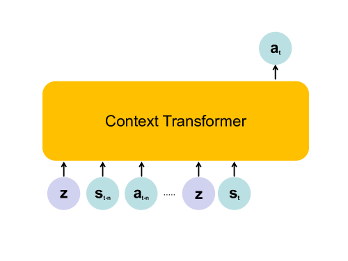
Figure 4: Our policy is a latent condtioned Decision Transformer, that is we utilize the contextual information as our goal to inference the sequence model.

And then, we detail the architecture of Contextual transformer we utilized, in our main context, we optimize the contextual policy, the contextual information is learned be Equation 22.

Given the HI extractor $I_{\phi}$, contextual embedding $\mathbf{z}^{*}$ and contextual policy $\pi_{\mathbf{z}}(\cdot|\tau^{\mathbf{z}}_{t-k:t})$, where $\tau^{\mathbf{z}}=\{\mathbf{z},\mathbf{s}_{0},\mathbf{a}_{0}\cdots,\mathbf{s}_{t},\mathbf{a}_{t}\}$ means the latent conditioned trajectory. We model the contextual policy based the aforementioned definition 4.1, definition 4.2 and we optimize the contextual policy using Equation 22 and Equation 23.

$$\small\begin{split}\mathcal{J}_{\mathbf{z}^{*}}=\min_{\mathbf{z}^{*},I_{\phi}}\mathbb{E}_{\tau^{*}\sim\pi^{*}(\tau)}[||\mathbf{z}^{*}-I_{\phi}(\tau^{*})||]-\mathbb{E}_{\hat{\tau}\sim\hat{\pi}}[||\mathbf{z}^{*}-I_{\phi}(\hat{\tau})||],\end{split}$$ (22)

where $\tau=\big{\{}\mathbf{s}_{0},\mathbf{a}_{0},\cdots,\mathbf{s}_{t},\mathbf{a}_{t}\big{\}}$ is the rollout trajectory, while $\hat{\pi}(\cdot|\tau)$ and $\pi^{*}(\cdot|\tau)$ are separated to the sub-optimal and optimal policies. Meanwhile, we also optimize the HI extractor $I_{\phi}(\cdot|\tau)$ via Equation 23.

$$\small\begin{split}\mathcal{J}_{\mathbf{z}^{*},I_{\phi}}=\min\limits_{\mathbf{z}^{*},I_{\phi}}\mathbb{E}_{\hat{\tau}\sim\hat{\pi}(\tau),\tau^{*}\sim\pi^{*}(\tau)}[||\mathbf{z}^{*}-I_{\phi}(\tau^{*})||-||\mathbf{z}^{*}-I_{\phi}(\hat{\tau})||]\end{split}$$ (23)

Appendix C Experimental Setup

C.1 Model Hyperarameters

The hyperparameter settings of our customed Decision Transformer is shown in Table 7. And the hyperparameters of our Encoder is shown in Table 8.

Hyparameter	$\rm Value$
DT
num layers	3
num heads	2
learning rate	1.2e-4
weight decay	1e-4
warmup steps	10000
activation	relu
z dim	16
value dim	64
dropout	0.1

Table 7: Hyparameters of our DT.

Hyparameter	$\rm Value$
Encoder (BERT)
num layers	3
num heads	8
learning rate	1.2e-4
weight decay	1e-4
warmup steps	10000
activation	relu
num embeddings	4096
z dim	16
value dim	64
dropout	0.1
d model	512
Decoder (MLP)
num layers	3
hidden dim	32
input (output) dim	1024

Table 8: Hyparameters of our VQ-VAE.

C.2 Computing Resources

Our experiments are conducted on a a computational cluster with multi-NVIDIA-A100 GPU (40GB), and NVIDIA-V100 GPU (80GB) cards for about 20 days.

C.3 Codebase

For more details about our approach, it can be refereed to Algorithm 2. Our source code is complished with the following projects: OPPO  , Decision Transformer . Additionally, our source code will be released at: .

Algorithm 2  

Require: HI extractor $I_{\phi}(\cdot|\tau)$, Contextual policy $\pi_{\mathbf{z}}(\cdot|\tau)$, sub-optimal offline datasets $D_{\hat{\tau}}\sim\hat{\pi}$, randomly initialized contextual embedding $\mathbf{z}^{*}$, and demonstrations (expert trajectories) $D_{\rm\tau^{*}}\sim\pi^{*}$

Training:

1:  Sample sub-optimal trajectory $\hat{\tau}$ from $\mathcal{D}_{\hat{\tau}}$, and sampling batch expert trajectory $\tau^{*}$ from $D_{\rm\pi^{*}}$.

2:  update $I_{\phi}$ by Equation 4 and Equation 5 and vq-loss (Appendix B, Equation 21). Update $\mathbf{z}^{*}$ by Equation 5.

3:  update $\pi_{\mathbf{z}}$ by Equation 4.

Evaluation:

1:  Initialize $t=0$; $\mathbf{s}_{t}\leftarrow\rm env.reset()$; $\tau_{\mathbf{z}^{*}}=\{\mathbf{z}^{*},\mathbf{s}_{0}\}$; ${\rm done}=\rm False$, $R=0$, $N=0$.

2:  while $t\leq N$ or not done do

3:    $\mathbf{a}_{t}\leftarrow\pi_{\mathbf{z}^{*}}(\cdot|\tau_{\mathbf{z}^{*}})$;

4:    $\mathbf{s}_{t+1},{\rm done},r_{t}\leftarrow\rm env.step(\mathbf{a}_{t})$;

5:    $\tau_{\mathbf{z}^{*}}.{\rm append}(\mathbf{a}_{t},\mathbf{z}^{*},\mathbf{s}_{t+1})$; t+=1

6:    $R+=r_{t}$

7:  end while

8:  Return $R$

C.4 Datasets

Gym Mujoco domain.

D4RL tasks in Gym mojoco domain are demonstrated in Figure 5, and the concrete information of these offline tasks are shown in table 9:

Dataset Name	Domain	Policy
hopper-expert-v2	Gym-Mujoco	SAC
walker2d-expert-v2	Gym-Mujoco	SAC
halfcheetah-expert-v2	Gym-Mujoco	SAC
ant-expert-v2	Gym-Mujoco	SAC
hopper-medium-expert-v2	Gym-Mujoco	SAC
walker2d-medium-expert-v2	Gym-Mujoco	SAC
halfcheetah-medium-expert-v2	Gym-Mujoco	SAC
ant-medium-expert-v2	Gym-Mujoco	SAC
hopper-medium-v2	Gym-Mujoco	SAC
walker2d-medium-v2	Gym-Mujoco	SAC
halfcheetah-medium-v2	Gym-Mujoco	SAC
ant-medium-v2	Gym-Mujoco	SAC
hopper-medium-replay-v2	Gym-Mujoco	SAC
walker2d-medium-replay-v2	Gym-Mujoco	SAC
halfcheetah-medium-replay-v2	Gym-Mujoco	SAC
ant-medium-replay-v2	Gym-Mujoco	SAC

Table 9: Our offline RL datasets from D4RL.

• expert dataset is collected by the interaction of expert policy with the environment. Typically, this level datasets have a capacity of around 1000K.

• medium-replay dataset includes all samples in the replay buffer during the training process of a policy till it reaches the Medium level (”Medium” means first training a soft-actor-critic (SAC) (Haarnoja et al., 2018) agent with early stopping at half performance of its upper bound.) and then use its replay buffer as the offline RL datasets. In particualr, replay buffer is kind of a container used for saving experience, and have to push $\{s,a,s^{\prime}\}$ at every interaction step. Typically, this level datasets have a capacity of around 10K.

• medium dataset is collected by rolling out medium SAC policy about 1e6 samples.

• medium-expert dataset is collected by mixture the datasets collected by medium and expert policy, the scale of medium-expert dataset is around 2e6 samples.

Figure 5: Demonstrations of Gym Mujoco tasks. From left to right, these agents are: Ant, HalfCheetah, Hopper respectively.

Maze2d Domain

The Maze2d domain (demonstrated in Figure 6) include a serious of navigation tasks in which a 2D agent is tasked with reaching a goal. This task is designed to offer a straightforward yet insightful evaluation of a policy’s capability to stitch sub-optimal trajectory fragments. Accordingly, a well-trained a policy equipped with stitching capability should be adept at finding the shortest path to the evaluation goal. Addtionally, The offline datasets for this task are generated by randomly selecting goal locations and using a planner to generate a sequence of waypoints. These waypoints are then followed using a PD controller. For more details of maze2d tasks, it can be refered to table 10.

Figure 6: Demonstrations of Gym Mujoco tasks. From left to right, these tasks are: maze2d-large-v1, maze2d-medium-v1, maze2d-umaze-v1, and maze2d-open-v0, respectively.

Dataset Name	Domain	Policy	Samples
maze2d-open-v0	Maze2d	Planner	$88592$
maze2d-medium-v1	Maze2d	Planner	$2*10^{6}$
maze2d-large-v1	Maze2d	Planner	$4*10^{6}$
maze2d-umaze-v1	Maze2d	Planner	$4*10^{6}$

Table 10: Our offline RL datasets from D4RL.

Appendix D A concise explanation of ContextFormer

In section 4, we conduct the mathematical derivation to indicate the necessary of endowing stitching to transformer by utilizing expert matching. Here we will provide a more concise explanation to illustrate why expert matching can assist in endowing the stitching capability to transformer for decision making.

we optimize the contextual policy by optimizing Equation 24.

$$\small\begin{split}\mathcal{J}_{\pi_{\mathbf{z}},I_{\phi}}=\mathbb{E}_{\tau\sim(\pi^{*},\hat{\pi})}[||\pi_{\mathbf{z}}(\cdot|I_{\phi}(\tau),\mathbf{s}_{0},\mathbf{a}_{0},\cdots,I_{\phi}(\tau),\mathbf{s}_{t})-\mathbf{a}_{t}||],\end{split}$$ (24)

where $\tau=\big{\{}\mathbf{s}_{0},\mathbf{a}_{0},\cdots,\mathbf{s}_{t},\mathbf{a}_{t}\big{\}}$ is the rollout trajectory, while $\hat{\pi}$ and $\pi^{*}$ are separated to the sub-optimal and optimal policies. Meanwhile, we also optimize the HI extractor $I_{\phi}$ and contextual embedding $\mathbf{z}^{*}$ via Equation 24 and 25.

$$\small\begin{split}\mathcal{J}_{\mathbf{z}^{*},I_{\phi}}=\min\limits_{\mathbf{z}^{*},I_{\phi}}\mathbb{E}_{\hat{\tau}\sim\hat{\pi}(\tau),\tau^{*}\sim\pi^{*}(\tau)}[||\mathbf{z}^{*}-I_{\phi}(\tau^{*})||-||\mathbf{z}^{*}-I_{\phi}(\hat{\tau})||]\end{split}$$ (25)

D.1 Perspective 1

The objective of Equation 25 aims to filter out the non-expert information in sub-optimal trajectories. And the extracted expert information will assist in the learning of expert HI, which is equivalent to augmenting expert trajectories, thereby helping to learn diverse expert skills, and showcase the enhancement of evaluation performance.

Explanation: When optimizing ContextFormer, we have two training objectives, namely Equations 24 and 25. Among that, Equation 24 ensures that $D(\mathbf{z}||I_{\phi}(\tau_{\mathbf{z}}))<\epsilon$, and Equation 25 ensures that $\mathbf{z}^{*}$ approaches the expert hindsight information (HI) $\textit{i}.\textit{e}.$ $I_{\phi}(\tau^{*})$ while moving away from the non-expert HI $\textit{i}.\textit{e}.$ $I_{\phi}(\hat{\tau})$. If $I_{\phi}(\hat{\tau})$ approaches $I_{\phi}(\tau^{*})$, it indicates that $||I_{\phi}(\hat{\tau})-\mathbf{z}^{*}||$ will yield a lower gradient, and such HI won’t be driven away from $\mathbf{z}^{*}$ so much. However, Equation 25 can drive $\mathbf{z}^{*}$ away from $I_{\phi}(\hat{\tau})$ where there is a distinct difference between $I_{\phi}(\hat{\tau})$ and $I_{\phi}(\tau^{*})$ (since $||I_{\phi}(\hat{\tau})-\mathbf{z}^{*}||$ will obtain a large gradient and $\min\mathcal{J}_{\mathbf{z}^{*},I_{\phi}}$ is equivalent to maximizing $||\mathbf{z}^{*}-I_{\phi}(\hat{\tau})||$). To summarize, $\mathbf{z}^{*}$ only deviate from HI where a significant difference exists between $I_{\phi}(\hat{\tau})$ and $I_{\phi}(\tau^{*})$, this approach helps exclude non-expert HI from $\hat{\tau}$.

On the other hand, we know that $D(\mathbf{z}||I_{\phi}(\tau_{\mathbf{z}}))<\epsilon$ implies that if we want to roll out $\tau_{\mathbf{z}}$, we simply need to provide $\mathbf{z}$ and the well-trained contextual policy $\pi_{\mathbf{z}}(\cdot|\tau)$. Given that $\mathbf{z}^{*}$ incorporates the HI of expert trajectories and $\hat{\tau}$ with expert HI, which indicates approximating $I_{\phi}(\tau^{*})$, $\mathbf{z}^{*}$ is associated with such capability that rolling out more diverse expert trajectories. This set includes $\{\tau^{*}\}$ and $\{\hat{\tau}|D(I_{\phi}(\hat{\tau})||\mathbf{z}^{*})<\epsilon\}$.

Connection with stitching:

Based on the preceding analysis, we can generate a variety of expert trajectories by jointly optimizing Equations 24 and 25. Intuitively, the newly generated trajectories include three conditional types: 1) expert+non-expert. 2) expert+expert. 3) non-expert+non-expert. If this contextual policy can effectively roll out optimal trajectories by stitching non-expert fragments, then the stitching process can be realized.

Appendix E Extended Experiments

E.1 Aggregated metrics with ContextFormer.

In order to demonstrate the significance of improvement brought by our approach, we conduct the statistical analysis via method mentioned by (Agarwal et al., 2022). As shown in Figure 7, our method can achieve competitive performance on both LfD and LfO settings.

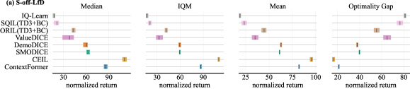
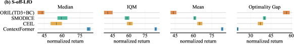
Figure 7: Aggregate metrics on D4RL with 95% CIs based on 12 benchmarks. In this experiment, we refer to the evaluation metric of (Agarwal et al., 2022) to report the performance of ContextFormer. Higher median, higher IQM, and higher mean and lower optimality gap are better. In particular, (a) Single domain LfD IL setting with 20 demos. (b) Single domain LfO IL setting with 20 demos.

References

- Agarwal et al. (2022) Agarwal, R., Schwarzer, M., Castro, P. S., Courville, A., and Bellemare, M. G. Deep reinforcement learning at the edge of the statistical precipice, 2022.
- An et al. (2021) An, G., Moon, S., Kim, J.-H., and Song, H. O. Uncertainty-based offline reinforcement learning with diversified q-ensemble, 2021.
- Argall et al. (2009) Argall, B. D., Chernova, S., Veloso, M., and Browning, B. A survey of robot learning from demonstration. Robotics and Autonomous Systems, 57(5):469–483, 2009. ISSN 0921-8890. doi: https://doi.org/10.1016/j.robot.2008.10.024. URL https://www.sciencedirect.com/science/article/pii/S0921889008001772.
- Boborzi et al. (2022) Boborzi, D., Straehle, C.-N., Buchner, J. S., and Mikelsons, L. Imitation learning by state-only distribution matching, 2022.
- Brantley et al. (2020) Brantley, K., Sun, W., and Henaff, M. Disagreement-regularized imitation learning. In International Conference on Learning Representations, 2020. URL https://openreview.net/forum?id=rkgbYyHtwB.
- Brockman et al. (2016) Brockman, G., Cheung, V., Pettersson, L., Schneider, J., Schulman, J., Tang, J., and Zaremba, W. Openai gym, 2016.
- Brown et al. (2020) Brown, D. S., Goo, W., and Niekum, S. Better-than-demonstrator imitation learning via automatically-ranked demonstrations. In Kaelbling, L. P., Kragic, D., and Sugiura, K. (eds.), Proceedings of the Conference on Robot Learning, volume 100 of Proceedings of Machine Learning Research, pp. 330–359. PMLR, 30 Oct–01 Nov 2020. URL https://proceedings.mlr.press/v100/brown20a.html.
- Chang et al. (2021) Chang, J., Uehara, M., Sreenivas, D., Kidambi, R., and Sun, W. Mitigating covariate shift in imitation learning via offline data with partial coverage. In Ranzato, M., Beygelzimer, A., Dauphin, Y., Liang, P., and Vaughan, J. W. (eds.), Advances in Neural Information Processing Systems, volume 34, pp. 965–979. Curran Associates, Inc., 2021. URL https://proceedings.neurips.cc/paper_files/paper/2021/file/07d5938693cc3903b261e1a3844590ed-Paper.pdf.
- Chen et al. (2021) Chen, L., Lu, K., Rajeswaran, A., Lee, K., Grover, A., Laskin, M., Abbeel, P., Srinivas, A., and Mordatch, I. Decision transformer: Reinforcement learning via sequence modeling, 2021.
- Chen et al. (2022) Chen, X., Ghadirzadeh, A., Yu, T., Gao, Y., Wang, J., Li, W., Liang, B., Finn, C., and Zhang, C. Latent-variable advantage-weighted policy optimization for offline rl, 2022.
- DeMoss et al. (2023) DeMoss, B., Duckworth, P., Hawes, N., and Posner, I. Ditto: Offline imitation learning with world models, 2023.
- Devlin et al. (2019) Devlin, J., Chang, M.-W., Lee, K., and Toutanova, K. Bert: Pre-training of deep bidirectional transformers for language understanding, 2019.
- Fu et al. (2019) Fu, J., Kumar, A., Soh, M., and Levine, S. Diagnosing bottlenecks in deep q-learning algorithms, 2019.
- Fu et al. (2020) Fu, J., Kumar, A., Nachum, O., Tucker, G., and Levine, S. D4rl: Datasets for deep data-driven reinforcement learning. ArXiv, abs/2004.07219, 2020. URL https://api.semanticscholar.org/CorpusID:215827910.
- Fu et al. (2021) Fu, J., Kumar, A., Nachum, O., Tucker, G., and Levine, S. D4rl: Datasets for deep data-driven reinforcement learning, 2021.
- Furuta et al. (2022) Furuta, H., Matsuo, Y., and Gu, S. S. Generalized decision transformer for offline hindsight information matching, 2022.
- Garg et al. (2022) Garg, D., Chakraborty, S., Cundy, C., Song, J., Geist, M., and Ermon, S. Iq-learn: Inverse soft-q learning for imitation, 2022.
- Gu et al. (2023) Gu, Y., Dong, L., Wei, F., and Huang, M. Pre-training to learn in context, 2023.
- Haarnoja et al. (2018) Haarnoja, T., Zhou, A., Abbeel, P., and Levine, S. Soft actor-critic: Off-policy maximum entropy deep reinforcement learning with a stochastic actor, 2018.
- Ho & Ermon (2016) Ho, J. and Ermon, S. Generative adversarial imitation learning. In Lee, D., Sugiyama, M., Luxburg, U., Guyon, I., and Garnett, R. (eds.), Advances in Neural Information Processing Systems, volume 29. Curran Associates, Inc., 2016. URL https://proceedings.neurips.cc/paper_files/paper/2016/file/cc7e2b878868cbae992d1fb743995d8f-Paper.pdf.
- Hong et al. (2023) Hong, J., Dragan, A., and Levine, S. Offline rl with observation histories: Analyzing and improving sample complexity, 2023.
- Hu et al. (2023) Hu, S., Shen, L., Zhang, Y., and Tao, D. Prompt-tuning decision transformer with preference ranking, 2023.
- Judah et al. (2014) Judah, K., Fern, A., Tadepalli, P., and Goetschalckx, R. Imitation learning with demonstrations and shaping rewards. Proceedings of the AAAI Conference on Artificial Intelligence, 28(1), Jun. 2014. doi: 10.1609/aaai.v28i1.9024. URL https://ojs.aaai.org/index.php/AAAI/article/view/9024.
- Kang et al. (2023) Kang, Y., Shi, D., Liu, J., He, L., and Wang, D. Beyond reward: Offline preference-guided policy optimization, 2023.
- Kim et al. (2022) Kim, G.-H., Seo, S., Lee, J., Jeon, W., Hwang, H., Yang, H., and Kim, K.-E. DemoDICE: Offline imitation learning with supplementary imperfect demonstrations. In International Conference on Learning Representations, 2022. URL https://openreview.net/forum?id=BrPdX1bDZkQ.
- Kostrikov et al. (2019) Kostrikov, I., Nachum, O., and Tompson, J. Imitation learning via off-policy distribution matching, 2019.
- Kostrikov et al. (2021) Kostrikov, I., Nair, A., and Levine, S. Offline reinforcement learning with implicit q-learning, 2021.
- Kumar et al. (2020) Kumar, A., Zhou, A., Tucker, G., and Levine, S. Conservative q-learning for offline reinforcement learning, 2020.
- Levine et al. (2020) Levine, S., Kumar, A., Tucker, G., and Fu, J. Offline reinforcement learning: Tutorial, review, and perspectives on open problems, 2020.
- Liu et al. (2023a) Liu, J., He, L., Kang, Y., Zhuang, Z., Wang, D., and Xu, H. Ceil: Generalized contextual imitation learning, 2023a.
- Liu et al. (2023b) Liu, J., Zu, L., He, L., and Wang, D. Clue: Calibrated latent guidance for offline reinforcement learning, 2023b.
- Liu et al. (2021) Liu, P., Yuan, W., Fu, J., Jiang, Z., Hayashi, H., and Neubig, G. Pre-train, prompt, and predict: A systematic survey of prompting methods in natural language processing, 2021.
- Liu et al. (2018) Liu, Y., Gupta, A., Abbeel, P., and Levine, S. Imitation from observation: Learning to imitate behaviors from raw video via context translation. In 2018 IEEE International Conference on Robotics and Automation (ICRA), pp. 1118–1125, 2018. doi: 10.1109/ICRA.2018.8462901.
- Ma et al. (2022) Ma, Y. J., Shen, A., Jayaraman, D., and Bastani, O. Versatile offline imitation from observations and examples via regularized state-occupancy matching, 2022.
- Paster et al. (2022) Paster, K., McIlraith, S., and Ba, J. You can’t count on luck: Why decision transformers and rvs fail in stochastic environments, 2022.
- Peng et al. (2019) Peng, X. B., Kumar, A., Zhang, G., and Levine, S. Advantage-weighted regression: Simple and scalable off-policy reinforcement learning, 2019.
- Ravichandar et al. (2020) Ravichandar, H., Polydoros, A. S., Chernova, S., and Billard, A. Recent advances in robot learning from demonstration. Annual Review of Control, Robotics, and Autonomous Systems, 3(1):297–330, 2020. doi: 10.1146/annurev-control-100819-063206. URL https://doi.org/10.1146/annurev-control-100819-063206.
- Reddy et al. (2019) Reddy, S., Dragan, A. D., and Levine, S. Sqil: Imitation learning via reinforcement learning with sparse rewards, 2019.
- Ross et al. (2011) Ross, S., Gordon, G., and Bagnell, D. A reduction of imitation learning and structured prediction to no-regret online learning. In Gordon, G., Dunson, D., and Dudík, M. (eds.), Proceedings of the Fourteenth International Conference on Artificial Intelligence and Statistics, volume 15 of Proceedings of Machine Learning Research, pp. 627–635, Fort Lauderdale, FL, USA, 11–13 Apr 2011. PMLR. URL https://proceedings.mlr.press/v15/ross11a.html.
- Sasaki & Yamashina (2021) Sasaki, F. and Yamashina, R. Behavioral cloning from noisy demonstrations. In International Conference on Learning Representations, 2021. URL https://openreview.net/forum?id=zrT3HcsWSAt.
- Schulman et al. (2017) Schulman, J., Wolski, F., Dhariwal, P., Radford, A., and Klimov, O. Proximal policy optimization algorithms, 2017.
- Torabi et al. (2019) Torabi, F., Warnell, G., and Stone, P. Recent advances in imitation learning from observation, 2019.
- Vamplew et al. (2021) Vamplew, P., Smith, B. J., Kallstrom, J., Ramos, G., Radulescu, R., Roijers, D. M., Hayes, C. F., Heintz, F., Mannion, P., Libin, P. J. K., Dazeley, R., and Foale, C. Scalar reward is not enough: A response to silver, singh, precup and sutton (2021), 2021.
- van den Oord et al. (2018) van den Oord, A., Vinyals, O., and Kavukcuoglu, K. Neural discrete representation learning, 2018.
- Wu et al. (2022) Wu, J., Wu, H., Qiu, Z., Wang, J., and Long, M. Supported policy optimization for offline reinforcement learning, 2022.
- Xu et al. (2022) Xu, M., Shen, Y., Zhang, S., Lu, Y., Zhao, D., Tenenbaum, J. B., and Gan, C. Prompting decision transformer for few-shot policy generalization, 2022.
- Yamagata et al. (2023) Yamagata, T., Khalil, A., and Santos-Rodriguez, R. Q-learning decision transformer: Leveraging dynamic programming for conditional sequence modelling in offline rl, 2023.
- Zhang et al. (2023) Zhang, W., Xu, H., Niu, H., Cheng, P., Li, M., Zhang, H., Zhou, G., and Zhan, X. Discriminator-guided model-based offline imitation learning. In Liu, K., Kulic, D., and Ichnowski, J. (eds.), Proceedings of The 6th Conference on Robot Learning, volume 205 of Proceedings of Machine Learning Research, pp. 1266–1276. PMLR, 14–18 Dec 2023. URL https://proceedings.mlr.press/v205/zhang23c.html.
- Zolna et al. (2020) Zolna, K., Novikov, A., Konyushkova, K., Gulcehre, C., Wang, Z., Aytar, Y., Denil, M., de Freitas, N., and Reed, S. Offline learning from demonstrations and unlabeled experience, 2020.