A Causal Model for Quantifying Multipartite Classical and Quantum Correlations

Abstract

We give an operational definition of information-theoretic resources within a given multipartite classical or quantum correlation. We present our causal model that serves as the source coding side of this correlation and introduce a novel concept of resource rate. We argue that, beyond classical secrecy, additional resources exist that are useful for the security of distributed computing problems, which can be captured by the resource rate. Furthermore, we establish a relationship between resource rate and an extension of Shannon’s logarithmic information measure, namely, total correlation. Subsequently, we present a novel quantum secrecy monotone and investigate a quantum hybrid key distribution system as an extension of our causal model. Finally, we discuss some connections to optimal transport (OT) problem.

I Introduction

Quantum entanglement and its connections to classical information have been the subject of continuous research, finding applications in diverse fields such as quantum key distribution (QKD), superdense coding, and distributed computing [1, 2, 3, 4, 5, 6, 7, 8, 9, 10, 11, 12]. One approach within QKD is entanglement-based QKD [13], where quantum entanglement is harnessed to achieve non-local effects and replace classical information. Especially in cryptographic tasks involving more than two parties, such as multipartite key distribution or conference key agreement, multipartite entanglement is utilized in different protocols [14, 15, 16, 17] and leads to a higher secret key rate than bipartite protocol [18]. Recent advances in fully connected quantum networks [19, 20] further facilitate the realization of these protocols.

The quantification of secrecy in multipartite cryptography poses a persistent challenge. Classical information quantification of a given probability, pioneered by Shannon in his seminal work [21], is inherently linked to logarithmic measures such as entropy and relative entropy. To measure how much secrecy can be provided by a classical or quantum correlation, Cerf et al. introduce the concept of secrecy monotone in [22]. Total correlation, an extension of Shannon’s logarithmic measures introduced by Watanabe [23], serves as one of these secrecy monotones. Its operational significance extends to various aspects, including the variational form of the optimal broadcast rate of the omniscient coordination problem [24] and the multivariate covering lemmas [25, 26]. Recent developments in device-independent QKD provide quantum versions of total correlation, offering an upper bound on the rate of conference key agreement [27, 28, 29].

Meanwhile, the discovery of causal-effect relations with a given correlation has been an important task in causality [30]. The problem of finding the minimal amount of resources to replicate a given effect, known as model preference and minimality in the context of causality, has also been extensively studied. This includes the study of the coordination problem in classical information theory [31, 32, 33, 26, 24] and the simulation of quantum measurements and quantum channels in quantum information theory [34, 35, 36, 37]. Notably, a concept called “the source coding side of problem” was introduced in [26], which relates a source coding problem to a given problem in classical information theory, such as channel coding and network information theory problems. Additionally, an intriguing causal perspective of quantum mechanics called indefinite causal order has been studied in [38, 39, 40, 41, 42, 43]. The equivalence between positive secrecy content and quantum correlation has been established in [12, 11, 10].

In this paper, the classical and quantum correlations we study refer to joint probabilities and entangled states, respectively. Our main focus is on understanding the information-theoretic resources offered by a given multipartite classical or quantum correlation, and we provide its lexical and formal definitions later in the paper. Following Reichenbach’s Common Cause Principle [44], we introduce a causal model where the correlation can be replicated by a set of common causes. These common causes are considered as mediums through which messages can be transmitted securely, allowing us to discover the information-theoretic resources that cannot measured by the classical secrecy measure. The minimal amount of the common causes is obtained following the same random binning techniques in [26] and defined as resource rate. Therefore, we call our model the source coding side of a given correlation.

Following the theoretical results, we further study a quantum hybrid network, where quantum resources are restricted to a set of quantum servers following bipartite protocols such as BB84 or E91. The motivation for this problem is that the current practical deployment of QKD links is still mainly limited to point-to-point connections, which does not allow the implementation of multipartite entanglement-based QKD schemes. As highlighted in previous research such as [45], the integration of bipartite keys into multipartite keys has been an ongoing challenge in both classical and quantum cryptography. We demonstrate that, when there are enough bipartite quantum keys buffered in each user, we can achieve multipartite key distribution by unicasting classical information with the rate of total correlation. Furthermore, in large-scale long-distance networks with distributed or decentralized topologies, the adoption of multi-hop communication and relay nodes becomes important to solve scalability issues [46]. The results also extend to scenarios involving multi-hop communications.

I-A Notations

Let $\mathcal{S}$ be a set, then $\mathcal{S}\backslash x$ denotes the set $\{s\in\mathcal{S}|s\neq x\}$. $\mathbb{R}_{+}$ denotes the set of positive real numbers. $\mathbb{N}_{+}$ denotes the set of positive natural numbers. $\mathbb{F}_{2}$ is the finite field with two elements. Let $\mathcal{X}$ be a discrete finite set. $\mathcal{X}^{n}$ denotes the $n$-ary Cartesian power set of $\mathcal{X}$. We write an element $x\in\mathcal{X}$ in lower-case letters and a random variable $X$ on $\mathcal{X}$ in capital letters. $X_{1:m}$ and $X^{n}_{1:m}$ denote sequences of random variables with the sizes of $m$ and $m\times n$. $X^{\otimes n}$ denotes a $n$-length sequence of i.i.d. random variables whose probability measure is given by the tensor product $\bigotimes^{n}_{i=1}P_{X_{i}}$. We define $X_{-j}$ as $X_{1:m}$ to remove the $j$-th element, i.e. $X_{-j}:=(X_{1},\cdots,X_{j-1},X_{j+1},\cdots,X_{m}),\forall j\in\mathcal{M}:=\{1,2,\cdots,m\}$. We denote $\Pi(\{P_{X_{j}}\}_{j=1}^{m})$ as the set of all probability measures supported on $\mathcal{X}_{1}\times\mathcal{X}_{2}\times\cdots\times\mathcal{X}_{m}$ with the marginal measures $\{P_{X_{j}}\}_{j=1}^{m}$. $\Pi_{j}P$ denotes the $j$-th marginal of a joint measure $P$. $H(\cdot)$, $I(\cdot;\cdot)$ and $\operatorname{TV}(\cdot,\cdot)$ denote entropy, mutual information, and total variation, respectively. $\delta_{x}$ is a Dirac measure at $x$. $\operatorname{epi}f$ is the epigraph of a function $f$. $a_{n}\doteq b_{n}$ means that $\lim_{n\rightarrow\infty}\frac{1}{n}\log\frac{a_{n}}{b_{n}}=0$. The occurrence of a sequence of events $A_{n}$ almost surely means that the probability $\lim_{n\rightarrow\infty}P(A_{n})=1$. $\delta>0$ denotes an infinitesimal term converging to zero when $\epsilon\rightarrow 0$ or $n\rightarrow\infty$. Let $\mathcal{H}$ be a Hilbert space. $\mathcal{S}(\mathcal{H})$ denotes the set of the density operators over $\mathcal{H}$.

II Preliminaries

This section gives an overview of multipartite quantum cryptography and secrecy monotone as well as a special case that supports our argument. Current studies on multipartite quantum cryptography primarily focus on Greenberger-Horne-Zeilinger (GHZ) state [47], which is a fundamental multipartite entangled state. The $m$-qubit GHZ state is written as

$$|\psi_{1}\rangle:=\frac{1}{\sqrt{2}}(|0\rangle^{\otimes m}+|1\rangle^{\otimes m}).$$ (1)

The corresponding quantum circuit is shown in Fig. 1. A $m$-qubit GHZ state exhibits instantaneous identical outcomes in $m$ subsystems when measured on computational bases. The outcome is written as a uniform probability on two vectors $\boldsymbol{0}$ and $\boldsymbol{1}$ with all entries of $0$ and $1$ respectively, i.e., $P^{(1)}_{X_{1:m}}:=\frac{1}{2}(\delta_{\boldsymbol{0}}+\delta_{\boldsymbol{1}})$. It allows a user in the system to broadcast one perfect secure bit with the remaining $m-1$ users [14]. The key with layered structure discussed in [15] is a tensor product of different GHZ states among different subsets of the whole set of users.

0 & H 1 [3]$\frac{|{000}\rangle+|{111}\rangle}{\sqrt{2}}$
0 1
0

Figure 1: Quantum circuit of 3-qubit GHZ state.

Next, we consider a quantum state mentioned in [22],

$$|\psi_{2}\rangle:=\frac{1}{2}(|000\rangle+|011\rangle+|101\rangle+|110\rangle).$$ (2)

Its corresponding quantum circuit is illustrated in Fig. 2. The measurement outcome on computational bases, i.e. $P^{(2)}_{X_{1:3}}:=\frac{1}{4}(\delta_{(000)}+\delta_{(011)}+\delta_{(101)}+\delta_{(110)})$, yields $X_{1},X_{2}\sim\mathrm{Bernoulli}(\frac{1}{2})$ as two independent random variables, while deterministic relationship $X_{3}=X_{1}\oplus X_{2}$ holds when all three are observed. Notably, these keys can be useful in a problem of distributed coding for computing [25], as shown in Fig.  3. The objective is to securely compute $Y_{3}=Y_{1}\oplus Y_{2}$ at the receiver, where $Y_{1}$ and $Y_{2}$ are distributed binary sources available at two different senders. $Y_{3}$ can be recovered from two encrypted bits $Y_{3}=M_{1}\oplus M_{2}\oplus X_{3}$, while the original sources $Y_{1}$ and $Y_{2}$ remain private. We can generalize (2) into higher dimension with $m\geq 3$. Let

$$|\psi_{3}\rangle:=2^{-\frac{m-1}{2}}\sum_{x_{1:m}\in\mathcal{X}_{1:m}}|x_{1:m}\rangle,$$ (3)

where $\mathcal{X}_{1:m}=\{x_{1:m}\in\mathbb{F}^{m}_{2}|\sum^{m}_{i=1}x_{i}=0\}$. This allows $m-1$ communications devices to securely transmit $m-1$ bits $Y_{1},\cdots,Y_{m-1}$ and compute a parity bit $Y_{m}=Y_{1}\oplus\cdots\oplus Y_{m-1}$. Such a computation has practical uses in error correction [48].

0 & H 2 [3]$\frac{|000\rangle+|011\rangle+|101\rangle+|110\rangle}{2}$
0 H 1
0

Figure 2: Quantum circuit of (2).

Figure 3: A problem of distributed coding for computing.

To measure the amount of secrecy in these joint probabilities, a secrecy monotone obeys (1) semi-positivity, (2) vanishing on product probability distributions, (3) monotonicity under local operations, (4) monotonicity under public communication, (5) additivity, and (6) continuity; see the formal definition in [22]. As one of the secrecy monotones, the total correlation of a given random variable $X_{1:m}$ is written as

$$C(X_{1:m}):=\int\log\frac{dP_{X_{1:m}}}{\prod_{i=1}^{m}dP_{X_{i}}}\,dP_{X_{1:m}},$$ (4)

where $X_{i}$ is the observed variables for subsystem $i\in\mathcal{M}:=\{1,2,\cdots,m\},m\in\mathbb{N}_{+}$. When $m=1$, we have $C=0$. When $m=2$, total correlation recovers mutual information $I(X_{1};X_{2})$. Cerf et al. also provide a quantum generalization of secrecy monotone for a quantum state $\rho$, written as

$$C_{\text{er}}(\rho):=\sum_{i=1}^{m}S(A_{i})-S(A_{1}\cdots A_{m}),$$ (5)

where $S(A_{i})$ is the von Neumann entropy of subsystem $A_{i},i\in\mathcal{M}$, and the whole quantum system is written as $A_{1}\cdots A_{m}$. Groisman et al. claim in [49] that $C_{\text{er}}$ measures the total amount of correlations, which includes the amount of quantum and classical correlations and equals the amount of randomness to decorrelate the state.

By considering the classical and quantum secrecy monotones of the above classical and quantum correlations, we observe that there are resources useful for an information-theoretic task that can be captured by $C_{\text{er}}$, but not by $C$. For $P^{(1)}_{X_{1:m}}$ and $|\psi_{1}\rangle$, $C=m-1$ and $C_{\text{er}}=m$. The total correlation corresponds to the $m-1$ received bits. The extra bit in $C_{\text{er}}$ is considered as the amount of quantum entanglement in [49], which is used to realize quantum phenomena such as non-locality and is therefore not considered as an information-theoretic resource. Let $P^{(3)}_{X_{1:m}}$ be the measurement outcome of $|\psi_{3}\rangle$ on computational bases. We have $C=1$ and $C_{\text{er}}=m$ for $P^{(3)}_{X_{1:m}}$ and $|\psi_{3}\rangle$. The total correlation still corresponds to the received bit for the distributed computing problem in Fig. 3. To give an interpretation of the extra $m-1$ bits in $C_{\text{er}}$, we perform the decorrelation process in [49] to $|\psi_{2}\rangle$, which can be easily extended to $|\psi_{3}\rangle$. We apply one of two unitary transformations $\mathbbm{1}$ or $\sigma_{z}$ with equal probability on the first qubit and obtain

$$\rho=\frac{1}{2}|\phi_{1}\rangle\langle\phi_{1}|+\frac{1}{2}|\psi_{2}\rangle\langle\psi_{2}|,$$ (6)

where

$$|\phi_{1}\rangle:=\frac{1}{2}(|000\rangle+|011\rangle-|101\rangle-|110\rangle).$$

We can write (6) as

$$\rho= \frac{1}{4}|0\rangle\langle 0|\otimes(|00\rangle+|11\rangle)(\langle 00|+\langle 11|)$$

$$+\frac{1}{4}|1\rangle\langle 1|\otimes(|01\rangle+|10\rangle)(\langle 01|+\langle 10|),$$

We further apply $\mathbbm{1}$ or $\sigma_{x}$ with equal probability on the first qubit and obtain

$$\frac{1}{2}\mathbbm{1}\otimes\frac{1}{4}[(|00\rangle+|11\rangle)(\langle 00|+\langle 11|)+(|01\rangle+|10\rangle)(\langle 01|+\langle 10|)].$$

Now the first qubit is disentangled with the last two qubits. We observe that the state of the last two qubits is a mixture of two maximally entangled states, i.e.,

$$\frac{1}{4}[(|00\rangle+|11\rangle)(\langle 00|+\langle 11|)+(|01\rangle+|10\rangle)(\langle 01|+\langle 10|)].$$ (7)

By applying $\mathbbm{1}$ or $\sigma_{z}$ with equal probability on the second qubit, we get the following disentangled three qubits,

$$\frac{1}{2}\mathbbm{1}\otimes\frac{1}{2}\mathbbm{1}\otimes\frac{1}{2}\mathbbm{1}.$$

In this process, we used three bits of randomness to disentangle $|\psi_{2}\rangle$. The amount of randomness is equal to $C_{\text{er}}(|\psi_{2}\rangle\langle\psi_{2}|)$. We note that (7) is the reduced density operator on $A_{2}A_{3}$. One bit of randomness is used in (7) to pair quantum states $|00\rangle$ with $|11\rangle$, and $|01\rangle$ with $|10\rangle$ in two subsystems. Consequently, $A_{1}$ can further employ one bit of randomness to establish the deterministic relationship $X_{3}=X_{1}\oplus X_{2}$ with the other two subsystems. However, any measurement outcomes on $A_{2}A_{3}$ are independent and $C(P^{(2)}_{X_{2:3}})=0$. We consider that most of the resources in $|\psi_{3}\rangle$ are used to coordinate the measurement outcomes on different marginals, in a form similar to 7, which cannot be measured by total correlation. This leads to the application in the distributed computing problem, where the goal is to coordinate between $m-1$ devices, and all the transmitted $m-1$ bits are necessary, even though the recovered information is only one bit. To quantify the additional resources that a multipartite entangled state can potentially provide, we introduce a causal model in the next section.

III A causal model for quantifying resources

In this section, we present our causal model as the source coding side of a multipartite correlation.

Definition 1 (Causal model of multipartite systems).

A causal model of a multipartite system is defined as a directed bipartite graph $G^{(n)}=(\Gamma,V,E)$, where $\Gamma$ and $V$ are two sets of vertices, $E$ is the set of edges and $n\in\mathbb{N}_{+}$. $\Gamma:=\{X_{1}^{n},X^{n}_{2},\cdots,X^{n}_{m}\}$ is the set of the observed variables, where each $X_{i}^{n}\in\mathcal{X}^{n}_{i}$ for $i\in\mathcal{M}$. $V:=\{\omega_{i,j}\}_{\forall i,j\in\mathcal{M},i\neq j}$ is the set of the latent variables, where each $\omega_{i,j}$ is a random variable supported on $\Omega_{i,j}$. Note that $\omega_{i,j}$ and $\omega_{j,i}$ refer to the same vertex. $E$ is the set of the edges joining only from $\omega_{i,j}$ to the corresponding $X_{i}^{n}$ and $X_{j}^{n}$. We denote $\omega_{i}:=\{\omega_{i,j}\}_{j\in\mathcal{M},j\neq i}$ as the set of the neighbors of $X_{i}^{n}$, which is supported on $\Omega_{i}\subset\Omega_{1,i}\times\cdots\times\Omega_{i-1,i}\times\Omega_{i,i+1}\times\cdots\times\Omega_{i,m}$.

For every node $X^{n}_{i}$, a structural equation $X^{n}_{i}=f_{i}:\Omega_{i}\times\mathcal{U}_{i}\rightarrow\mathcal{X}^{n}_{i}$ holds, where $u_{i}\in\mathcal{U}_{i}$. $\Theta^{(n)}:=\{f_{i}(\omega_{i},u_{i})\}_{i\in\mathcal{M}}$ is the set of the structural equations. We define $R_{i,j}(G^{(n)},\Theta^{(n)}):=\log|\Omega_{i,j}|/n$ and $R(G^{(n)},\Theta^{(n)}):=\sum_{i,j}\log|\Omega_{i,j}|/n$ as the rate of the model.

Figure 4: A causal model with four observed variables and six latent variables.

The causal model and structural equation in Definition 1 were introduced in the general topic of causality (see, e.g., [30]). $\omega_{i,j}$ is the common cause of the two subsystems $i,j$, and $u_{i}$ is a local term at subsystem $i$. To discuss its interpretation, we provide an example that has been realized in [20, 17].

Example 1.

Consider four entangled photons that are sent to different locations and subsequently measured. The entangled photons display correlations between different locations, and this phenomenon can be described by the causal model in Fig. 4, where $\Gamma:=\{X^{n}_{1},X^{n}_{2},X^{n}_{3},X^{n}_{4}\}$ and $V:=\{\omega_{1,2},\omega_{1,3},\omega_{2,3},\omega_{1,4},\omega_{2,4},\omega_{3,4}\}$. Assume that the measurements are performed on the marginals in their natural order. Following the measurement outcomes $X_{1}^{n}$ and $X_{2}^{n}$, quantum non-locality is represented as the latent variable $\omega_{1,2}$ shared between marginals 1 and 2. Following $X_{3}^{n}$, we obtain $\omega_{1,3}$ and $\omega_{2,3}$. Following $X_{4}^{n}$, we obtain $\omega_{1,4},\omega_{2,4}$ and $\omega_{3,4}$.

In the above example, for each step $i+1$, $\omega_{1:i,i+1}$ is determined once the quantum measurements $\{E_{x_{1:i}}\}$ and $\{E_{x_{i+1}}\}$ are given. Because $\omega_{i+1,i+2:m}$ is determined by both $E_{x_{1:i+1}}$ and the future measurements, from the no-signaling principle, we know that the existing correlation between $X^{n}_{1:i}$ and $X^{n}_{i+1}$ is independent with the further measurements given $\{E_{x_{1:i}}\}$ and $\{E_{x_{i+1}}\}$. Therefore, we introduce a condition to characterize the no-signaling condition, i.e. $I(\omega_{1:i};\omega_{i+1,i+2:m}|\omega_{1:i,i+1})=0,i\in\{1,\cdots,m-1\}$; see also similar conditions in [29]. Then,

$$I(\omega_{1:i};\omega_{i+1}|\omega_{1:i,i+1})= I(\omega_{1:i};\omega_{i+1})-I(\omega_{1:i};\omega_{1:i,i+1})$$ (8)

$$= I(\omega_{1:i};\omega_{i+1})-H(\omega_{1:i,i+1})$$ (9)

$$= 0,$$ (10)

where (8) is from chain rule, and (9) is from the fact that the common elements between $\omega_{1:i-1}$ and $\omega_{1:i-1,i}$ are just $\omega_{1:i-1,i}$. We further allow the relationship (10) to tolerate a permutation, written as $\iota:\mathcal{M}\rightarrow\mathcal{M}$, which represents the possible order that the photons are measured. To define the amount of randomness with the above-mentioned properties, we give the next definition.

Definition 2 (Compatibility of a causal model).

We say a sequence of models $\{(G^{(n)},\Theta^{(n)})\}_{n}$ is compatible with $X_{1:m}$, if it satisfies the following conditions,
(Condition 1)   $\mathbb{E}_{\Theta^{(n)}}[\operatorname{TV}(P_{X^{n}_{1:m}},P_{X_{1:m}}^{\otimes n})]<\epsilon_{n}$, where $\lim_{n\rightarrow\infty}\epsilon_{n}=0$.
(Condition 2)   There exists a permutation $\iota:\mathcal{M}\rightarrow\mathcal{M}$ such that $I(\omega_{\iota(i+1)};\omega_{\iota(1):\iota(i)})=H(\omega_{\iota(i+1),\iota(1):\iota(i)}),i\in\{1,\cdots,m-1\}$. $I(\{\omega_{i,j}\}_{i,j};\{u_{i}\}_{i})=0,I(u_{i};u_{j})=0,\forall i,j$.

Note that there always exists a $\{(G^{(n)},\Theta^{(n)})\}$ that is compatible with an arbitrary $P_{X_{1:m}}$, as we can simply let $\omega_{i,j}=X^{\otimes n}_{1:m}$, $\forall i,j$ and the structural equation as the mapping from $X^{\otimes n}_{1:m}$ to $X^{\otimes n}_{i}$. Condition 1 characterizes the output statistics associated with a given correlation and is defined in the same way as in previous existing literature [31, 32, 33, 26, 24]. Conditions 2 can be considered as an information-theoretic extension of the causal order given in [40, 41, 42], where the amount of randomness between different marginals is further taken into account. Based on this definition, we further define resource rate.

Definition 3 (Resource rate for a classical correlation).

Given a sequence $\{(G^{(n)},\Theta^{(n)})\}$, we define $R(\{(G^{(n)},\Theta^{(n)})\}):=\limsup_{n\rightarrow\infty}R(G^{(n)},\Theta^{(n)})$ as its rate. We define $R^{*}(X_{1:m}):=\inf R(\{(G^{(n)},\Theta^{(n)})\})$ as the resource rate for $P_{X_{1:m}}$, where the infimum is among the sequences compatible with $P_{X_{1:m}}$. A sequence of models $\{(G^{(n)},\Theta^{(n)})\}$ compatible with $P_{X_{1:m}}$ is said to be optimal if $\lim_{n\rightarrow\infty}R(G^{(n)},\Theta^{(n)})=R^{*}(X_{1:m})$.

To simplify notation, we will use $(G,\Theta)$ and $\epsilon$ to refer to the sequences $\{(G^{(n)},\Theta^{(n)})\}$ and $\epsilon_{n}$, respectively, in the following text. We also use the term “step” as a synonym for the classical causal order.

IV Overview of main results

In Section II, we show the existence of the additional resources that cannot be measured by the classical measure through specific examples. In Section III, we motivate the causal model from a quantum perspective. In this section, we discuss how the causal model quantifies the resource in a general correlation. Now, let us provide a lexical definition for the information-theoretic resource under consideration in this paper. The information-theoretic resource in a given correlation is the amount of randomness at one location that has an effect at another location. Formally, the amount of resources is defined as the resource rate in Definition 2. The “one to another” condition in the lexical definition corresponds to Condition 2 in Definition 2. To ensure that the randomness has a real effect, we use infimum in Definition 2 to make sure it is necessary. To further look into this definition, we show that the proposed causal model characterizes the following three phenomena:

(a)

(b)

(c)

(d)

(e)

(f)

(g)

Figure 5: Consider the optimal compatible models of a 4-qubit GHZ state with a natural order. Replace the causal forks $X^{n}_{i}\leftarrow\omega_{i,j}\rightarrow X^{n}_{j}$ with an undirected edge if there is identical randomness in the latent variables and remove other forks. The resulting graph forms a spanning tree as shown in LABEL:sub@fig:g1 to LABEL:sub@fig:g6. For a sub-optimal model, there exist redundant latent variables, forming a circle when added to the spanning tree, as illustrated in LABEL:sub@fig:g7.

1. Identical randomness in different steps: Consider the example of a 4-qubit GHZ state in (1) where there is identical randomness shared by multiple marginals for broadcast traffic. In a group of users expected to share the same broadcast message, identical randomness of secrecy should cover them with a connected graph, and each pair of users within the group can be connected with a path. As illustrated in Fig. 5, this is represented as the latent variables with identical randomness. Only one marginal shares the randomness with another at each step in the optimal models. Each spanning tree corresponds to an optimal model.

2. Identical randomness in one step: In some cases, redundancy can exist in the latent variables. For example, consider the scenario shown in Fig. 5g, where marginals 2 and 3 share the same randomness with marginal 4 within one step. Compared to the other cases in Fig. 5, this case results in an extra edge being added to the spanning tree, thus forming a circle. This redundancy can be eliminated by the Slepian-Wolf coding technique, which forms a tree-like structure for identical randomness.

3. Vanishing randomness in one step: Consider the distributed computing problem in Fig. 3, where two bits of information can be securely transmitted, while only one bit can be recovered from the receiver. This arises from the algebraic property given by the binary addition, and we consider the difference between the sent information and the received information as the vanishing information. Similar to the distributed computing problem, two bits of latent variables need to be non-local, while the structural equation recovers only one bit of randomness at each marginal in the optimal causal model compatible with $P^{(2)}_{X_{1:3}}$, which we considered as vanishing randomness. The vanishing randomness also corresponds to the resource used to coordinate the measurement outcomes on different marginals in the form of (7).

We claim that the vanishing randomness is exactly the reason that a certain amount of resources cannot be measured by (4). We observe that (4) is well-defined as long as a $\sigma$-algebra on its support set can be specified. However, more mathematical structures are required on the support set when considering the linear algebraic formulation of quantum mechanics and the group operation in the distributed computing problem. We refer to these general properties as algebraic properties. Because of these additional mathematical structures, the quantification of multipartite entanglement remains a consistently challenging problem, and the explicit form of the optimal rate is unknown in general distributed coding of computing problems [25]. We show that our causal model can capture some of these algebraic properties and represent them as latent variables. We now provide an informal overview of our main results. We define $R_{\text{rec}}$ as the classical secrecy rate that can recover the same rate of classical message in Subsection V-B. Then, we have the next theorem:

Theorem.

For a given joint probability $P_{X_{1:m}}$, we have

$$R_{\text{rec}}(X_{1:m})\stackrel{{\scriptstyle\textnormal{(a)}}}{{\mathstrut{\leq}}}C(X_{1:m})\stackrel{{\scriptstyle\textnormal{(b)}}}{{\mathstrut{\leq}}}R^{*}(X_{1:m}).$$

The results related to this theorem are presented in Section V. In particular, the resource rates for $P^{(1)}_{X_{1:m}}$ and $P^{(3)}_{X_{1:m}}$ are both $m-1$, representing the amount of information that can be securely transmitted.

The condition to determine whether there is vanishing randomness in a model compatible with $P_{X_{1:m}}$ can be written as an expression in Theorem 2, i.e., $H(\omega_{i}|X^{n}_{i})\leq n\delta,\exists\delta,\forall i$. This means that if this expression holds, the observed variable can almost surely recover the latent variable inversely at each marginal. In this case, the resource rate becomes the total correlation. The amount of vanishing randomness is represented as the gap in the inequality (Theorem); see also Theorem 3. Therefore, the operational meaning of total correlation becomes the amount of information-theoretic resources removing the amount of vanishing randomness. Moreover, when we “use” the latent variables to transmit messages, the message that is carried by the amount of vanishing randomness cannot be recovered at the receiver, which gives the inequality (Theorem).

Next, we consider the amount of resources that can be provided by a quantum state. We define quantum total correlation $C_{Q}(\rho)$ and quantum rate $R^{*}_{Q}(\rho)$ in Section VI as the supremum of $C$ and $R^{*}$ that can be provided by a given state $\rho$ among all possible POVMs, respectively. Following the argument in [49] that $C_{\text{er}}$ is the total amount of the correlations, we obtain the second expression as follows:

Theorem.

For a given pure state $\rho$, and for all $i\in\mathcal{M}$, we have

$$C_{Q}(\rho)\leq R^{*}_{Q}(\rho)\leq C_{\text{er}}(\rho)-S(A_{i}).$$

The results related to this theorem are presented in Section VI. Inherited from the classical results, the quantum resource rates for $|\psi_{1}\rangle$ and $|\psi_{3}\rangle$ are also $m-1$, quantifying the amount of information that can be securely transmitted. Additionally, we show that $C_{Q}(\rho)$ is a quantum secrecy monotone. We demonstrate that these two quantities are consistent with the von Neumann entropy of bipartite pure state in Proposition 2, and their monotonicity in Proposition 3. We prove in Theorem 5 that quantum total correlation lower bounds the number of controlled gates in a quantum circuit.

As an extension of the causal model, Section VII introduces a variant of the omniscient coordination problem [24] with unicast traffic in a quantum hybrid system, as illustrated in Fig. 6. We show that its optimal rate is exactly the total correlation. Section VIII provides two slightly different rate-distortion settings of the hybrid system, with their optimal coding schemes corresponding to the two multivariate covering lemmas in [25, 26], respectively. In Section VIII-C, we review a linear programming problem and motivate it in a cryptanalysis problem. We show in Proposition 10 that total correlation characterizes the condition of the extremal points.

Figure 6: A centralized quantum hybrid key distribution system with $\alpha_{1}$ as the quantum server. $\alpha_{1}$ possesses independent bipartite keys with users indexed as $\{1,\cdots,m\}$. We show that $\alpha_{1}$ can securely and efficiently establish a multipartite key with secrecy equivalent to a classical correlation $P_{X_{1:m}}$ by unicasting classical information to the users with the rate of total correlation.

Finally, Sections IX and X contain some experimental results, discussion, and conclusions.

V Analysis of causal models

In this section, we study the properties of the optimal rate and its connections to total correlation. Additionally, we demonstrate that total correlation serves as an upper bound of the classical secrecy rate. We first show in Lemma 1 that total correlation can be decomposed into a sum of mutual information when $m\geq 3$.

Lemma 1.

$$C(X_{1:m})=\sum_{i=1}^{m-1}I(X_{i+1};X_{1:i}).$$ (11)

Proof.

We can decompose $C(X_{1:m})$ as follows,

$$C(X_{1:m})$$

$$= \int\log\frac{dP_{X_{1:m}}}{dP_{X_{m}}\,dP_{X_{1:m-1}}}+\log\frac{dP_{X_{1:m-1}}}{\prod_{i=1}^{m-1}dP_{X_{i}}}\,dP_{X_{1:m}}$$

$$= I(X_{m};X_{1:m-1})+C(X_{1:m-1})$$ (12)

$$= \sum_{i=1}^{m-1}I(X_{i+1};X_{1:i}),$$ (13)

where (13) is obtained by repeating (12) successively. ∎

The total variation in Condition 1 characterizes the weak convergence of probability measures. Therefore, we can state the following lemma.

Lemma 2.

[50] Suppose $P$ and $Q$ are two probability measures on discrete finite support $\mathcal{X}$ such that $\operatorname{TV}(P,Q)<\epsilon$ with $\epsilon<\frac{1}{2}$. Then

$$|H(P)-H(Q)|<\epsilon\log|\mathcal{X}|+\epsilon\log\epsilon.$$ (14)

Lemma 2 gives that the logarithmic information measures for these two nearly identical measures will also be nearly identical. Furthermore, the nearly identical relationship, $\operatorname{TV}(P,Q)<\epsilon$, will hold under the same transition matrix on these two measures [26].

In the next theorem, we show the first connection between total correlation and the resource rate.

Theorem 1 (Total correlation lower bounds the optimal rate).

$$R^{*}(X_{1:m})\geq C(X_{1:m}).$$ (15)

Proof.

For a given $(G,\Theta)$, we have

$$nR(G,\Theta):= n\sum_{i,j}R_{i,j}$$

$$\geq \sum_{i=1}^{m-1}H(\omega_{\iota(i+1),\iota(1):\iota(i)})$$ (16)

$$= \sum_{i=1}^{m-1}I(\omega_{\iota(i+1)};\omega_{\iota(1):\iota(i)})$$ (17)

$$\geq \sum_{i=1}^{m-1}I(X^{n}_{i+1};X^{n}_{1:i})$$ (18)

$$= C(X^{n}_{1:m})$$ (19)

$$\geq n(C(X_{1:m})-\delta),$$ (20)

where (16) is from the fact that the range of $\omega_{\iota(i+1),\iota(1):\iota(i)}$ is at most $\sum_{j=1}^{i}R_{i+1,j}$, (17) is from Condition 2, (18) is from data processing inequality, (19) is from Lemma 1, and (20) is from Condition 1 and Lemma 2. Because $\delta$ is an infinitesimal converging to zero and $R(G,\Theta)$ is defined by limit supremum, we know that $R(G,\Theta)\geq C(X_{1:m})$. From the definition of infimum, we further obtain (15). ∎

Using Theorem 1, we can conclude that the optimal rate for GHZ state measurement outcomes in (1) aligns with its total correlation, i.e. $m-1$. However, as exemplified in (2), we observe that the optimal rate may exceed the total correlation. To address this issue, we provide the following definition of the typical set and state a theorem.

Definition 4 (Typical set [25]).

Let $x^{n}\in\mathcal{X}^{n}$ be a sequence with length $n$, where $\mathcal{X}$ is a finite alphabet. The typical set $\mathcal{T}^{(n)}_{\epsilon}(X)$ of a given pmf $P_{X}$ and $\epsilon\in(0,1)$ is defined as follows:

$$\mathcal{T}^{(n)}_{\epsilon}(X):=\{x^{n}\in\mathcal{X}^{n}:|\pi(x|x^{n})-P_{X}(x)|\leq\epsilon\cdot P_{X}(x)\},$$ (21)

where the empirical pmf $\pi(\cdot|x^{n}):\mathcal{X}\rightarrow\mathbb{R}_{+}$ of a given sequence $x^{n}$ is defined as

$$\pi(x|x^{n}):=\frac{|\{i:x_{i}=x\}|}{n}.$$ (22)

By applying the law of large numbers, it can be observed that $P(X^{\otimes n}\in\mathcal{T}^{(n)}_{\epsilon}(X))\rightarrow 1$ and $P(x^{n})\doteq 2^{-nH(X)},\forall x^{n}\in\mathcal{T}^{(n)}_{\epsilon}(X)$ when $X\sim P_{X}$ and $n\rightarrow\infty$. We can now provide intuition on random binning, which will be used in Theorem 2 and Proposition 6. Given finite alphabets $\mathcal{X}_{1:m}$ and a pmf $P_{X_{1:m}}$, let $\iota_{i}:\mathcal{X}^{n}_{i}\rightarrow\Omega_{i}:=\{1,\cdots,2^{nR_{i}}\},i\in\mathcal{M}$ be a set of independent randomly selected mappings. According to Slepian-Wolf theorem [51], $\iota_{1:m}$ is one-to-one almost surely, i.e., $P\big{(}x^{n}_{1:m}=x^{\prime n}_{1:m}|\iota_{1:m}(x^{n}_{1:m})=\iota_{1:m}(x^{\prime n}_{1:m})\big{)}\rightarrow 1$ for almost all $x^{n}_{1:m},x^{\prime n}_{1:m}\in\mathcal{T}^{(n)}_{\epsilon}(X_{1:m})$, when $n\rightarrow\infty$ and

$$\sum_{i\in\Gamma}R_{i}\geq H(X_{\Gamma}|X_{\mathcal{M}\backslash\Gamma})+\delta,\forall\Gamma\subset\mathcal{M}.$$ (23)

Particularly, when $\sum_{i\in\mathcal{M}}R_{i}=H(X_{1:m})+\delta$, the extracted random variables $\omega_{1:m}$ are nearly independent, i.e., $I(\omega_{i};\omega_{j})\leq n\delta,\forall i\neq j$; see also [52, Lemma 13.13].

We next provide a necessary and sufficient condition for the bound (15) to be tight in the following theorem.

Theorem 2.

If there exists a $(G,\Theta)$ that is compatible with $P_{X_{1:m}}$ and satisfies $H(\omega_{i}|X^{n}_{i})\leq n\delta,\exists\delta,\forall i$, then the following equation holds necessarily and sufficiently:

$$R^{*}(X_{1:m})=C(X_{1:m}).$$ (24)

Proof.

We first show the sufficiency. Without loss of generality, we assume that $\iota$ in Condition 2 is an identity map. Let $\omega_{i,j}$ be the latent variable from the existing model $(G,\Theta)$ that is compatible with $P_{X_{1:m}}$ and satisfies $H(\omega_{i}|X^{n}_{i})\leq n\delta$. From Condition 2, we have Markov chain $\omega_{1:i-1}-\omega_{1:i-1,i}-\omega_{i}$. Moreover, for $i<j$, we have

$$H(\omega_{i,j}|\omega_{1:i-1,j})\geq H(\omega_{i,j}|\omega_{1:i-1})$$

$$= H(\omega_{i,j}|\omega_{1:i-1,i}),$$ (25)

where (25) is from the Markov property. Let $\omega^{\prime}_{i,j}$ be the set of Slepian-Wolf code for the sequences of the latent variables $\omega^{n}_{i,j}\sim P^{\otimes n}_{\omega_{i,j}}\in\mathcal{T}^{(n)}_{\epsilon}(\omega_{i,j})$ as illustrated in Fig. 7, whose rates $R_{i,j}:=H(\omega_{i,j}|\omega_{1:i-1,j})+\delta$, for $i<j$, and can be written as follows,

$$R_{1,2}-\delta=H(\omega_{1,2}),$$

$$R_{1:2,3}-\delta=H(\omega_{1,3}),H(\omega_{2,3}|\omega_{1,3}),$$

$$R_{1:3,4}-\delta=H(\omega_{1,4}),H(\omega_{2,4}|\omega_{1,4}),H(\omega_{3,4}|\omega_{1:2,4}),$$

$$\cdots$$

$$R_{1:m-1,m}-\delta=H(\omega_{1,m}),\cdots,H(\omega_{m-1,m}|\omega_{1:m-2,m}).$$

Each $\omega^{\prime}_{i,j}$ is obtained from the following process.
Step 1: Generate $\omega^{n}_{1}\sim P^{\otimes n}_{\omega_{1}}$. Randomly bin $\omega^{n}_{1,j}\in\mathcal{T}^{(n)}_{\epsilon}(\omega_{1,j})$ to $\omega^{\prime}_{1,j}$ at marginal 1, for $j=2,\cdots,m$.
Step 2: Recover $\omega^{n}_{1,2}$ from $\omega^{\prime}_{1,2}$ at marginal 2. If the mapping is not one-to-one, assign $\omega^{\prime}_{1,2}$ to a random value. Generate $\omega^{n}_{2}$ from the recovered $\omega^{n}_{1,2}$ according to the Markov property from (10). Randomly bin $\omega^{n}_{2,j}\in\mathcal{T}^{(n)}_{\epsilon}(\omega_{2,j})$ to $\omega^{\prime}_{2,j}$, for $j=3,\cdots,m$. We then apply this process sequentially.
Step $i$: Recover $\omega^{n}_{1:i-1,i}$ from $\omega^{\prime}_{1:i-1,i}$ at marginal $i$. If the mapping is not one-to-one, assign $\omega^{\prime}_{1:i-1,i}$ to a random value. Generate $\omega^{n}_{i}$ from the recovered $\omega^{n}_{1:i-1,i}$ according to the Markov property from (10). Randomly bin $\omega^{n}_{i,j}$ to $\omega^{\prime}_{i,j}$, $j=i+1,\cdots,m$.

(a) Step 1

(b) Step 2

(c) Step 3

Figure 7: Sequential Slepian-Wolf coding for redundancy elimination. Randomly selected mappings extract nearly independent $\omega^{\prime}_{1,3}$ and $\omega^{\prime}_{2,3}$ from correlated $\omega^{n}_{1,3}$ and $\omega^{n}_{2,3}$, respectively, at step 2, and extract nearly independent $\omega^{\prime}_{1,4}$, $\omega^{\prime}_{2,4}$ and $\omega^{\prime}_{3,4}$ from correlated $\omega^{n}_{1,4}$, $\omega^{n}_{2,4}$ and $\omega^{n}_{3,4}$, respectively, at step 3.

This process gives that $I(\omega^{\prime}_{i+1};\omega^{\prime}_{1:i})=H(\omega^{\prime}_{1:i,i+1})$. Additionally, we have that

$$\sum_{j\in\mathcal{M}\backslash i}R_{i,j}-(m-1)\delta$$

$$= \sum_{j=1}^{i-1}H(\omega_{j,i}|\omega_{1:j-1,i})+\sum_{j=i+1}^{m}H(\omega_{i,j}|\omega_{1:i-1,j})$$

$$= H(\omega_{1:i-1,i})+\sum_{j=i+1}^{m}H(\omega_{i,j}|\omega_{1:i-1,j})$$ (26)

$$\geq H(\omega_{1:i-1,i})+\sum_{j=i+1}^{m}H(\omega_{i,j}|\omega_{1:i-1,i})$$ (27)

$$\geq H(\omega_{i}),$$ (28)

where (26) and (28) are from chain rule, and (27) is from (25). With small modifications, we can further observe that the above-constructed rates satisfy (23) for each $\{R_{i,j}\}_{j\in\mathcal{M}\backslash i}$. By Slepian-Wolf theorem, $\omega^{\prime}_{i,j}$ recovers $\omega_{1:m}^{n}\in\mathcal{T}^{(n)}_{\epsilon}(\omega_{1:m})$ almost surely with the same probability, and let $\iota_{i}$ be the one-to-one mapping between most elements between $\omega^{\prime}_{i}$ and $\omega^{n}_{i}$. Assign the remaining infinitesimal probability mass to $\{\omega^{\prime}_{i,j}\}$ following Condition 2. Let $\{\omega^{\prime}_{i,j}\}$ and $\{f_{i}\circ\iota_{i}\}$ be the latent variables and structural equations of a new model. We know that the new model is still compatible with $P_{X_{1:m}}$. According to the assumption $H(\omega_{i}|X^{n}_{i})\leq n\delta$, we have

$$I(X^{n}_{i+1};\omega_{1:i}|X^{n}_{1:i})\leq\sum_{i=1}^{m}H(\omega_{i}|X^{n}_{i})\leq m\cdot n\delta,$$ (29)

and

$$I(\omega_{1:i};\omega_{i+1}|X^{n}_{i+1})\leq H(\omega_{i+1}|X^{n}_{i+1})\leq n\delta.$$ (30)

We can then obtain

$$I(X^{n}_{i+1};X^{n}_{1:i})+(m+1)\cdot n\delta$$

$$\geq I(X^{n}_{i+1};X^{n}_{1:i})+I(X^{n}_{i+1};\omega_{1:i}|X^{n}_{1:i})+n\delta$$ (31)

$$= I(X^{n}_{i+1};\omega_{1:i})+n\delta$$ (32)

$$\geq I(X^{n}_{i+1};\omega_{1:i})+I(\omega_{1:i};\omega_{i+1}|X^{n}_{i+1})$$ (33)

$$= I(\omega_{i+1};\omega_{1:i}),$$ (34)

where (31) is from (29), (33) is from (30), (32) and (34) are from the chain rule. Consequently, we have

$$R(G^{\prime},\Theta^{\prime})= \frac{1}{n}\sum_{i,j}R_{i,j}$$

$$= \frac{1}{n}(C(\omega_{1:m})+\delta^{\prime})$$

$$\leq \frac{1}{n}(C(X^{n}_{1:m})+n\delta^{\prime\prime})$$ (35)

$$\leq C(X_{1:m})+\delta^{\prime\prime\prime},$$ (36)

where (35) is from (34) and (36) is from Condition 1. Therefore, the bound in Theorem 1 is tight. If $\exists i,\forall\delta,H(\omega_{i}|X^{n}_{i})>n\delta$, we have

$$C(\omega_{1:m})$$

$$= C(\omega_{-i})+I(\omega_{i};\omega_{-i})$$

$$= C(\omega_{-i})+I(X^{n}_{i};\omega_{-i})+I(\omega_{i};\omega_{-i}|X^{n}_{i})$$

$$= C(\omega_{-i})+I(X^{n}_{i};\omega_{-i})+H(\omega_{i}|X^{n}_{i})$$ (37)

$$> C(X^{n}_{-i})+I(X^{n}_{i};X^{n}_{1:m-1})+n\delta$$ (38)

$$\geq n(C(X_{1:m})+\delta),$$ (39)

where (37) is from the fact that the common element between $\omega_{i}$ and $\omega_{-i}$ is just $\omega_{i}$ itself, (38) is from data processing inequality and (39) is from the fact that the condition $H(\omega_{i}|X^{n}_{i})>n\delta$ holds for all infinitesimal $\delta$. Therefore, (18) in Theorem 1 is not tight, and the rate would be strictly larger than $C(X_{1:m})$. The necessity is shown. ∎

Remark 1.

To discuss the interpretation of sequential Slepian-Wolf coding, we note that for the $i$-th step, $\omega^{\prime}_{1:i-1,i}$ represents the randomness that already exists and has been received by the $i$-th marginal, while $\omega^{\prime}_{i,i+1:m}$ represents the newly generated randomness sent by the $i$-th marginal to others. Hence, the resource rate also coincides with the rate of classical information needed to be sequentially transmitted between different marginals to recover the nearly identical effect as the joint probability $P_{X_{1:m}}$.

We notice from the proof that, once the latent variables $\omega_{i,j}$ of a sub-optimal model with an arbitrary causal order are given, the Slepian-Wolf code always achieves the rate $C(\omega_{1:m})+\delta$, whose expression is independent with the causal order. The marginal condition $H(\omega_{i}|X^{n}_{i})\leq n\delta$ further ensures that $C(\omega_{1:m})$ approaches $nC(X_{1:m})$. The condition $H(\omega_{i}|X^{n}_{i})\leq n\delta$ guarantees that the latent variable does not vanish when it is observed. This condition may not hold in the optimal compatible model for general probabilities, such as the one stipulated by (2). Thus, we define $R^{*}-C(X_{1:m})$ as the resource rate that vanishes on the marginals of the optimal model. Since $R^{*}$ is the rate of the latent variables in our model, we can always find another $\Theta^{\prime}$ whose structural equations are all bijective, allowing us to observe all the latent variables on the marginals. We formally prove this statement in Theorem 3.

Theorem 3.

Let $(G,\Theta)$ be an optimal model that is compatible with $P_{X_{1:m}}$ and approaches the rate $R^{*}$. Let $\Theta^{\prime}=\{f_{i}^{\prime}\}_{i=1}^{m}:\Omega_{i}\times\mathcal{U}_{i}\rightarrow\mathcal{X}^{\prime n}_{i}$ be a set of structural equations that are bijective with respect to $\omega_{i}$ and satisfy $H(X_{i}^{n}|\omega_{i})=H(X^{\prime n}_{i}|\omega_{i})$, where $X^{\prime n}_{i}:=f_{i}^{\prime}(\omega_{i},u_{i})$. Then the following relationship always holds:

$$R^{*}-C(X_{1:m})=\lim_{n\rightarrow\infty}\frac{1}{n}\sum_{i=1}^{m}H(X^{\prime n}_{i})-\sum_{i=1}^{m}H(X_{i}).$$ (40)

Proof.

We have

$$H(X^{\prime n}_{1:m})= H(X^{\prime n}_{1:m},\omega_{1:m})$$ (41)

$$= H(\omega_{1:m})+H(X^{\prime n}_{1:m}|\omega_{1:m})$$

$$= H(\omega_{1:m})+\sum_{i}H(X^{\prime n}_{i}|\omega_{i})$$ (42)

$$= H(\omega_{1:m})+\sum_{i}H(X^{n}_{i}|\omega_{i})$$ (43)

$$= H(\omega_{1:m})+H(X^{n}_{1:m}|\omega_{1:m})$$ (44)

$$= H(X^{n}_{1:m},\omega_{1:m}),$$ (45)

where (41) is from the bijection, (42) and (44) are because $u_{i}$ is local, and (43) is from the assumption. According to the fact that the model is optimal, there is no redundancy in the randomness of $\omega_{1:m}$. Thus, from (45) we have

$$|H(X^{n}_{1:m},\omega_{1:m})-H(X^{n}_{1:m})|= |H(X^{\prime n}_{1:m})-H(X^{n}_{1:m})|$$

$$\leq n\delta.$$ (46)

Given the optimal $\omega_{i,j}$, we know that the inequality (16) is tight according to Theorem 2. Thus,

$$n(R^{*}+\delta)= \sum_{i=1}^{m-1}I(\omega_{\iota(i+1)};\omega_{\iota(1):\iota(i)})$$

$$= C(\omega_{\iota(1):\iota(m)})$$

$$= \sum_{i=1}^{m}H(X^{\prime n}_{i})-H(X^{\prime n}_{1:m}),$$ (47)

where (47) is from (4) and the fact that $f^{\prime}_{i}$ is bijective. Furthermore, we have

$$2^{n\sum_{i=1}^{m}H(X_{i})-nC(X_{1:m})}\doteq 2^{H(X^{n}_{1:m})}$$ (48)

$$\doteq 2^{H(X^{\prime n}_{1:m})}$$ (49)

$$\doteq 2^{-nR^{*}+\sum_{i=1}^{m}H(X^{\prime n}_{i})},$$ (50)

where (48) is from (4) and Lemma 2, (49) is from (46), and (50) is from (47). (50) leads to

$$|R^{*}-C(X_{1:m})-\frac{1}{n}\sum_{i=1}^{m}H(X^{\prime n}_{i})+\sum_{i=1}^{m}H(X_{i})|\leq\delta.$$ (51)

Because $\delta$ is infinitesimal, the limit of $\frac{1}{n}\sum_{i=1}^{m}H(X^{\prime n}_{i})$ exists. ∎

We note that the assumption $H(X_{i}^{n}|\omega_{i})=H(X^{\prime n}_{i}|\omega_{i})$ implies that the amount of local randomness in the two models is identical. Such models can always be constructed.

V-A A special case: distributed computing

Next, we consider a special case of the causal model and recover the distributed coding for the computing problem in Fig. 3. We can give a proposition in this case.

Proposition 1.

Given independent $X_{1:m-1}$ such that $X_{m}=f(X_{1:m-1})$ and $H(X_{i}|X_{-i})=0,\forall i$, we have $R^{*}(X_{1:m})=\sum_{i=1}^{m-1}H(X_{i})$.

Proof.

According to Condition 2 and $H(X_{i}|X_{-i})=0$, we have $H(X^{n}_{i}|X^{n}_{-i})=H(X^{n}_{i}|\omega_{i})\leq n\delta$ and $H(X^{n}_{1:m-1}|\omega_{1:m})\leq\sum_{i=1}^{m-1}H(X^{n}_{i}|\omega_{i})\leq n\delta^{\prime}$ for a model compatible with $X_{1:m}$. Then, we have $H(\omega_{1:m})\geq n(H(X_{1:m-1})-\delta^{\prime})=n\sum_{i=1}^{m-1}H(X_{i})-n\delta^{\prime}$. This gives the converse. For the achievability, simply let $\omega_{i,m}$ be the source code of $X^{n}_{i},\forall i$, which leads to $R^{*}=\sum_{i=1}^{m-1}H(X_{i})$. ∎

We note that the conditions given in Proposition 1 encompass general distributed computing problems with a linear function on additive groups. In this case, the independent $X_{1:m-1}$ serves as the key for the transmitted messages. Then, there always exists a function $f$ letting $X^{n}_{m}$ be the key that is sufficient to decode the computing result according to the commutativity of the groups.

V-B Secret key problem

This subsection is motivated by the fact that not all resources can be effectively used as a key for recovering classical messages. We show that the rate of recovered messages is no larger than the total correlation, and therefore our results do not contradict previous results on classical information theory. We first formalize the secret key problem. Assume that $\mathcal{I}\subset\mathcal{M}$ is the set of the senders and $\mathcal{I}^{c}:=\mathcal{M}\backslash\mathcal{I}$ is the set of the receivers. For $i\in\mathcal{I}$ and $j\in\mathcal{I}^{c}$, we denote $M_{i,j}$ as the message that $i$ sends to $j$. The receiver recovers its information $Y^{n}_{j}=g_{j}(M_{\mathcal{I},j},X^{n}_{j})\in\mathcal{Y}^{n}_{j}$ for all the possible distributions on $\mathcal{Y}^{n}_{j}$, where $X^{n}_{j}$ is the $j$-th marginal of a joint key $X^{n}_{1:m}$ satisfying $\operatorname{TV}(P_{X^{n}_{1:m}},P_{X^{\otimes n}_{1:m}})<\epsilon$ with a given $X_{1:m}$. We assume $I(Y^{n}_{j};M_{\mathcal{I},\mathcal{I}^{c}})\leq n\delta$ and $H(X_{j}|X_{\mathcal{I}})=0$, which means that the information leakage when the message is wiretapped is almost zero, and the randomness of decryption is determined by the randomness of encryption. Let $R(\mathcal{Y}^{n}_{\mathcal{I}^{c}}):=\liminf_{n\rightarrow\infty}\frac{1}{n}\sum_{j\in\mathcal{I}^{c}}\log|\mathcal{Y}^{n}_{j}|$ be the rate of a sequence of alphabets. We define $R_{\text{rec}}(X_{1:m}):=\sup R(\mathcal{Y}^{n}_{\mathcal{I}^{c}})$ be the classical secrecy rate, where the supremum is among all the sequences of the alphabets and all $\mathcal{I}$ satisfying the given conditions of secure communication. Then we have the next theorem.

Theorem 4.

$$C(X_{1:m})\geq R_{\text{rec}}(X_{1:m}).$$ (52)

Proof.

Let $Y^{n}_{j}$ be uniform on $\mathcal{Y}^{n}_{j}$. The assumption $I(Y^{n}_{j};M_{\mathcal{I},\mathcal{I}^{c}})\leq n\delta$ implies $H(Y^{n}_{j})-H(Y^{n}_{j}|M_{\mathcal{I},\mathcal{I}^{c}})\leq n\delta$. Thus

$$\log|\mathcal{Y}^{n}_{j}|= H(Y^{n}_{j})$$

$$\leq H(Y^{n}_{j}|M_{\mathcal{I},\mathcal{I}^{c}})+n\delta$$

$$\leq H(X^{n}_{j})+n\delta,$$ (53)

where (53) is from data processing inequality. Then

$$\sum_{j\in\mathcal{I}^{c}}\log|\mathcal{Y}^{n}_{j}|\leq \sum_{j\in\mathcal{I}^{c}}H(X^{n}_{j})+n\delta^{\prime}$$ (54)

$$= \sum_{j\in\mathcal{I}^{c}}I(X^{n}_{j};X^{n}_{\mathcal{I}})+n\delta^{\prime\prime}$$ (55)

$$\leq nC(X_{1:m})+n\delta^{\prime\prime\prime},$$ (56)

where (54) is from (53), (55) is from $H(X^{n}_{j}|X^{n}_{\mathcal{I}})=0$, and (56) is from Lemma 1. ∎

Here we consider the security of the received message to encompass the distributed computing problems mentioned in Fig. 3, thus generalizing the bound of conference key agreement in [53, Theorem 4]. Theorem 4 states that total correlation of a system must not be smaller than the rate of the received messages. Similar statements can be made for systems in which the user acts as both sender and receiver through time division, and for systems with eavesdroppers; see the formal statement and proof in Appendix A. The bound (52) is tight in the cases of (1) and (3). This bound still holds when there are further local operations and classical public communications (LOPC). This is known as the monotonicity of secrecy monotone [22]. Let $m=2$ and $\mathcal{I}=\{1\}$. In this case, our problem recovers the secret key agreement problem in [26] and the key rate achieves $I(X_{1};X_{2})$ using random binning.

VI Quantifying multipartite entanglement

An immediate observation is that the joint keys $X^{n}_{1:m}$ compatible with $P_{X_{1:m}}$ can be equivalently achieved using a set of independent and identical multipartite quantum states with the same measurement outcome. This allows us to establish a mapping from the quantum state to the classical correlation. In this context, we quantify the entanglement by considering the largest amount of total correlation or resource rate obtained from all possible measurements of the quantum state. The quantum version of total correlation can be further shown to follow the properties of quantum secrecy monotones in [22]. We give our definition of quantum total correlation as follows.

Definition 5 (Quantum total correlation).

Given a density operator $\rho\in\mathcal{S}(\mathcal{H}_{1}\times\cdots\times\mathcal{H}_{m})$, its quantum total correlation is defined as

$$C_{Q}(\rho):=\max_{\{E_{x_{j}}\}_{x_{j},j\in\mathcal{M}}}C(X_{1:m}),$$ (57)

where $\{E_{x_{j}}\}_{x_{j},j\in\mathcal{M}}$ is a set of POVMs on the $j$-th marginal and $P_{X_{1:m}}$ is given by

$$P_{X_{1:m}}(x_{1:m})=\operatorname{tr}(\rho E_{x_{1}}\otimes E_{x_{2}}\otimes\cdots\otimes E_{x_{m}}).$$ (58)

The set of all possible POVMs forms a compact set because it is a Hilbert space with linear constraints. The objective function of (57) is continuous from the chain rule and the continuity of entropy. Thus, the maximum exists according to Weierstrass’ extreme value theorem. According to Theorem 4 and the monotonicity of total correlation in [22], we know that the quantum total correlation must be not smaller than the classical secrecy rate that can be extracted.

We can define the quantum resource rate as follows.

Definition 6 (Quantum resource rate).

Let $P_{X_{1:m}}$ be the measurement outcome of $\rho$ given in Definition 5. We denote the quantum resource rate as

$$R^{*}_{Q}(\rho):=\sup_{\{E_{x_{j}}\}_{x_{j},j\in\mathcal{M}}}R^{*}(X_{1:m}).$$ (59)

$R^{*}_{Q}$ preserves several properties of $R^{*}$. Notably, the same effect as that achieved by the measurement outcome of $\rho$ can be achieved by transmitting classical information if and only if the rate of the classical information is not smaller than $R^{*}_{Q}$, as discussed in Remark 1.

Next, we show that, similar to Theorem 1, the quantum total correlation lower bounds the quantum rate.

Corollary 1.

$$C_{Q}(\rho)\leq R^{*}_{Q}(\rho).$$ (60)

Proof.

Following Theorem 1, we have $C_{Q}(\rho)\leq R^{*}(X_{1:m})$ for the corresponding $P_{X_{1:m}}$ of $C_{Q}(\rho)$. Because $R^{*}_{Q}(\rho)$ is the supremum, we have $R^{*}(X_{1:m})\leq R^{*}_{Q}(\rho)$. ∎

The bound (60) is tight when the corresponding $P_{X_{1:m}}$ of $R^{*}_{Q}(\rho)$ satisfies the condition in Theorem 2. Specifically, for a separable pure state $|\psi\rangle=|\psi_{1}\rangle\otimes\cdots\otimes|\psi_{m}\rangle$, we can see that $C_{Q}(\rho)=R^{*}_{Q}(\rho)=0$, where $\rho:=|\psi\rangle\langle\psi|$, from the definition of tensor product. For a bipartite pure state, it can be immediately shown that $R^{*}_{Q}(\rho)$ and $C_{Q}(\rho)$ coincide with the von Neumann entropy of its reduced state by Schmidt decomposition, which was introduced to quantify bipartite entanglement, driven by applications like entanglement distillation and dilution [54]. We prove it formally in the next proposition.

Proposition 2.

Let $m=2$. Let $\rho:=|\psi\rangle\langle\psi|$ for a given $|\psi\rangle\in\mathcal{H}_{1}\times\mathcal{H}_{2}$. Let $\lambda_{i}$ be the Schmidt co-efficients of $|\psi\rangle$. We have $C_{Q}(\rho)=R^{*}_{Q}(\rho)=-\sum_{i=1}^{K}|\lambda_{i}|^{2}\log|\lambda_{i}|^{2}$.

Proof.

Assume that the dimensions of $\mathcal{H}_{1}$ and $\mathcal{H}_{2}$ are $K$ and $K^{\prime}$ respectively, where $K\leq K^{\prime}$. From Schmidt decomposition, we have $|\psi\rangle=\sum_{i=1}^{K}\lambda_{i}|i_{1}\rangle\otimes|i_{2}\rangle$, where $|i_{1}\rangle\in\mathcal{H}_{1}$ and $|i_{2}\rangle\in\mathcal{H}_{2}$ are the orthogonal bases. Given arbitrary two sets of POVMs $\{E_{x_{k_{1}}}\}$ and $\{E_{x_{k_{2}}}\}$, we have spectral decomposition $E_{x_{k_{1}}}=\sum_{j=1}^{K}a_{k_{1},j}|j_{1,k_{1}}\rangle\langle j_{1,k_{1}}|$ and $E_{x_{k_{2}}}=\sum_{j=1}^{K^{\prime}}b_{k_{2},j}|j_{2,k_{2}}\rangle\langle j_{2,k_{2}}|$, where $|j_{1,k_{1}}\rangle$ and $|j_{2,k_{2}}\rangle$ are the orthonormal eigenvectors. We know that the measurement outcome $\boldsymbol{P}(k_{1},k_{2})=\operatorname{tr}(\rho E_{x_{k_{1}}}\otimes E_{x_{k_{2}}})$. Define $\operatorname{diag}{(|\lambda_{i}|^{2})}$ as the square diagonal matrix with the diagonal entries of $|\lambda_{i}|^{2}$. Let $A$ and $B$ be the matrices with the entries of $\sum_{j=1}^{K}a_{k_{1},j}|\langle i_{1}|j_{1,k_{1}}\rangle|^{2}$ and $\sum_{j=1}^{K^{\prime}}b_{k_{2},j}|\langle i_{2}|j_{2,k_{2}}\rangle|^{2}$ respectively. We have $\boldsymbol{P}(k_{1},k_{2})=A\operatorname{diag}{(|\lambda_{i}|^{2})}B^{\intercal}$. Because $A$ and $B$ are both transition probability matrices, the maximal $C(X_{1:2})$ is $-\sum_{i=1}^{K}|\lambda_{i}|^{2}\log|\lambda_{i}|^{2}$ from data processing inequality. Let $\omega_{1,2}$ be the source code of the random variable with the probability $|\lambda_{i}|^{2}$. It can be shown that there always exists a model compatible with $\boldsymbol{P}(k_{1},k_{2})$. Therefore, $C_{Q}(\rho)=R^{*}_{Q}(\rho)$. ∎

For the multipartite case, we can provide an upper bound for the quantum rate.

Corollary 2.

For a given pure state $\rho=|\psi\rangle\langle\psi|$ and $\forall i\in\mathcal{I}$, we have

$$R^{*}_{Q}(\rho)\leq C_{\text{er}}(\rho)-S(A_{i}).$$ (61)

Proof.

WLOG, we assume that $i=1$. For a pure state, we have $C_{\text{er}}:=\sum^{m}_{j=1}S(A_{j})$. From Proposition 2, we know that the latent variable with the rate $S(A_{j})$ is sufficient to establish any correlation given by the measurement outcome between $A_{j}$ and $A_{-j}$. Therefore, we let $R_{1,j}=S(A_{j})$ for $j=\{2,3,\cdots,m\}$ and let the other rates be zero, which is enough to recover the correlation. $I(\omega_{i+1};\omega_{1:i})=H(\omega_{i+1,1:i})$ holds because there is only one element $\omega_{1,i+1}$ in $\omega_{i+1}$. ∎

When $|\psi_{1}\rangle$ and $|\psi_{3}\rangle$ are measured on computational bases, the classical non-local rates become $m-1$ according to Section V. We have $R^{*}_{Q}=m-1=C_{\text{er}}(\rho)-S(A_{i})$ for $|\psi_{1}\rangle$ and $|\psi_{3}\rangle$ because the bound (61) is tight in this case. Therefore, $R^{*}_{Q}$ quantifies the amount of information that can be securely transmitted in these two cases. We also provide an example to show that (61) is not always tight. Let

$$|\psi_{4}\rangle:=\frac{1}{2}(|00\rangle+|11\rangle)\otimes(|00\rangle+|11\rangle).$$ (62)

The von Neumann entropy on each marginal is one, thus $C_{\text{er}}(\rho)-S(A_{i})=3$. However, the identical effect can be achieved by two bits of latent variables.

It can also be shown that the quantum rate and quantum total correlation are non-increasing under local operations.

Proposition 3 (Monotonicity of quantum rate and quantum total correlation).

Suppose $\mathcal{E}_{j}$ is a trace-preserving quantum operation on $j$-th marginal. Let $\rho^{\prime}:=\mathcal{E}\rho\mathcal{E}^{\dagger}$, where $\mathcal{E}:=I_{1}\otimes\cdots\otimes\mathcal{E}_{j}\otimes\cdots\otimes I_{m}$. We have

$$R^{*}_{Q}(\rho^{\prime})\leq R_{Q}(\rho)\text{ and }C_{Q}(\rho^{\prime})\leq C_{Q}(\rho).$$ (63)

Proof.

Let $E_{x_{1}},\cdots,E_{x_{m}}$ be the optimal measurements for $R^{*}_{Q}(\rho^{\prime})$. Let $E^{\prime}_{x_{j}}:=\mathcal{E}_{j}E_{x_{j}}\mathcal{E}^{\dagger}_{j}$. We have

$$P_{X^{\prime}_{1:m}}(x_{1:m}):= \operatorname{tr}(\mathcal{E}\rho\mathcal{E}^{\dagger}E_{x_{1}}\otimes E_{x_{2}}\otimes\cdots\otimes E_{x_{m}})$$

$$= \operatorname{tr}(\rho E_{x_{1}}\otimes\cdots E^{\prime}_{x_{j}}\otimes\cdots\otimes E_{x_{m}}),$$ (64)

where (64) is from the cyclic property of trace. Then we know that $E_{x_{1}},\cdots,E^{\prime}_{x_{j}}$, $\cdots,E_{x_{m}}$ form a set of suboptimal measurements for $R^{*}_{Q}(\rho)$ from (64). We have that $R^{*}_{Q}(\rho^{\prime})=R^{*}(P_{X^{\prime}_{1:m}})\leq R^{*}_{Q}(\rho)$ because $R^{*}_{Q}$ is defined by maximization. The same steps also hold for $C_{Q}(\rho)$. ∎

Up to now, we can see that $C_{Q}(\rho)$ follows the conditions of quantum secrecy monotones except for the continuity from the above discussion; see [22] for the formal definition of quantum secrecy monotone. Next, we show the continuity.

Proposition 4.

$C_{Q}(\rho)$ is continuous w.r.t. $\rho$.

Proof.

Let $d(\cdot,\cdot)$ be a metric for density operators. Let $\rho^{\prime}$ be a density operator such that $d(\rho,\rho^{\prime})<\epsilon$. Let $\{E_{x_{j}}\}$ be the optimal measurements for $\rho$ in (57). Let $X^{\prime\prime}_{1:m}$ be the measurement outcome of $\rho^{\prime}$ with $\{E_{x_{j}}\}_{j\in\mathcal{M}}$. We have $C_{Q}(\rho)-C(X^{\prime\prime}_{1:m})<\epsilon^{\prime}$ from the continuity of entropy and linear operators on Hilbert space. Because $C_{Q}(\rho^{\prime})$ is obtained from maximization, we know that $C_{Q}(\rho)<C(X^{\prime\prime}_{1:m})+\epsilon^{\prime}\leq C_{Q}(\rho^{\prime})+\epsilon^{\prime}$. Let $X^{\prime}_{1:m}$ be the measurement outcome of $\rho$ with the optimal POVM $\{E_{x^{\prime}_{j}}\}$ for $\rho^{\prime}$. Following the same way, we have $0<C_{Q}(\rho^{\prime})-C(X^{\prime}_{1:m})<\epsilon^{\prime\prime}$, then $C_{Q}(\rho^{\prime})<C(X^{\prime}_{1:m})+\epsilon^{\prime\prime}\leq C_{Q}(\rho)+\epsilon^{\prime\prime}$. ∎

Next, we show the operational meaning of quantum total correlation from another perspective. When we describe a quantum system, a commonly used model is the quantum circuit. In quantum circuits, entanglement is usually introduced by CNOT gates, which can also be observed from Fig. 1 and Fig. 2. Research has shown that CNOT gate is the only multi-qubit operation required in a universal set of quantum gates to approximate any unitary operation with arbitrary accuracy [55]. In the next theorem, we show that the number of CNOT gates is also related to quantum total correlation.

Theorem 5.

Suppose we have a quantum circuit where a multi-qubit operation is simply a set of CNOT gates. The circuit can be written as a mapping from the input state to the output state, i.e., $|0\rangle^{\otimes m}\rightarrow|\psi\rangle\in\mathbb{C}^{2^{m}}$. Let $\rho=|\psi\rangle\langle\psi|$. The number of CNOT gates is not smaller than $C_{Q}(\rho)$.

Proof.

Let $T$ be the number of CNOT gates. Let $\rho^{(t)}$ be the quantum state that passes through the $t$-th CNOT gate but before the $(t+1)$-th CNOT gate. If parallel gates exist, we note that they can always be separated into different steps. Let $X^{(t)}_{1:m}$ be the measurement outcome using the optimal measurement for $\rho^{(t)}$. We have $C_{Q}(\rho^{(0)})=0$ because of the initial state $|0\rangle^{\otimes m}$. For $t+1>0$, let $i$ be the target qubit index. We have

$$C_{Q}(\rho^{(t+1)})= I(X^{(t+1)}_{i};X^{(t+1)}_{-i})+C(X^{(t+1)}_{-i})$$ (65)

$$\leq I(X^{(t+1)}_{i};X^{(t+1)}_{-i})+C(X^{(t)}_{-i})$$ (66)

$$\leq I(X^{(t+1)}_{i};X^{(t+1)}_{-i})+C_{Q}(\rho^{(t)})$$

$$\leq 1+C_{Q}(\rho^{(t)}),$$ (67)

where (65) is from Lemma 1, (66) is from the fact that only controlled gates increase $C_{Q}(\rho)$ according to Theorem 3, and (67) is from the fact that $X_{i}$ has binary support. Therefore, $C_{Q}(\rho^{(T)})-C_{Q}(\rho^{(0)})\leq T$. ∎

We can see immediately that, using the same steps, Theorem 5 also applies to other controlled gates with one target qubit; see, e.g., [56] for the expression of general controlled gates. Using the general controlled gate, the number of controlled gates in Fig. 2 can be reduced to one.

So far we have presented results related to the information-theoretic resource in both classical and quantum correlations. In the next section, we will study a hybrid system that combines quantum and classical information.

VII Extensions to hybrid systems

In this section, we derive the results related to the quantum hybrid system given in Fig. 6.

VII-A Asymptotic equivalence

First, we notice that the nearly i.i.d. condition given in Definition 2 is quite strict. We begin by providing a looser definition of asymptotic equivalence, which yields the same level of secrecy, which we elaborate on later.

Definition 7 (Asymptotic equivalence).

We say a sequence of random variables $X^{n}_{1:m}$ supported on $\mathcal{X}^{(n)}_{1:m}\subset\mathcal{T}_{\epsilon}^{(n)}(X_{1:m})$ is asymptotically equivalent to $P_{X_{1:m}}$, if $P(x^{n}_{1:m})\doteq 2^{-nH(X_{1:m})}$, $\forall x^{n}_{1:m}\in\mathcal{X}^{(n)}_{1:m},\epsilon\in(0,1)$, when $n\rightarrow\infty$. If there exists another $X^{\prime n}_{1:m}$ such that $\operatorname{TV}(P_{X^{n}_{1:m}},P_{X^{\prime n}_{1:m}})<\epsilon$ and $X^{n}_{1:m}$ is asymptotically equivalent to $P_{X_{1:m}}$, we say that $X^{\prime n}_{1:m}$ is asymptotically equivalent to $P_{X_{1:m}}$ almost surely.

Definition 7 constrains the components of a random variable to be nearly equiprobable in typical sets, without requiring the probability measure to converge to $P^{\otimes n}_{X_{1:m}}$. We can observe that a sequence satisfying Condition 1 in Definition 2 is asymptotic equivalence to $P_{X_{1:m}}$ almost surely. We can also provide an example to show the implication of this definition.

Example 2.

Let $X^{\otimes n}_{1:m}$ be the i.i.d. measurement outcome of $\rho_{1}^{\otimes n}$ given in (1). Let $X^{n}_{1:m}$ be another random variable, only its first bit is different from $X^{\otimes n}_{1:m}$, i.e., let $X_{1:m,1}$ be a constant. For $x^{n}_{1:m}$ such that $P_{X^{n}_{1:m}}(x^{n}_{1:m})>0$, we have $\frac{1}{2}P_{X^{n}_{1:m}}(x^{n}_{1:m})=P_{X^{\otimes n}_{1:m}}(x^{n}_{1:m})$ and $\operatorname{TV}(P_{X^{n}_{1:m}},P_{X^{\otimes n}_{1:m}})=\frac{1}{2}$. Therefore, $X^{n}_{1:m}$ is not nearly i.i.d. but it is asymptotically equivalent to $X_{1:m}$. Moreover, we know that $X^{n}_{1:m}$ provides $n-1$ bits of secret key and $\lim_{n\rightarrow\infty}\frac{n-1}{n}=1$. We consider that $X^{\otimes n}_{1:m}$ and $X^{n}_{1:m}$ have the same level of secrecy.

Using this definition, we can demonstrate that the asymptotic equipartition properties remain almost the same as those of $X^{\otimes n}_{1:m}$. We first show that a conditional typicality lemma holds for Definition 7; see [25] for the definition of conditional typical set.

Lemma 3.

Given two subsets $\Gamma,\Gamma^{\prime}\subset\mathcal{M}$ and $X^{n}_{1:m}$ satisfying Definition 7, we have

$$|H(X^{n}_{\Gamma^{\prime}}|X^{n}_{\Gamma})-nH(X_{\Gamma^{\prime}}|X_{\Gamma})|\leq n\delta,$$ (68)

and the expected cardinality

$$\mathbb{E}_{X^{n}_{\Gamma}}[|\{x^{n}_{\Gamma^{\prime}}|(x^{n}_{\Gamma^{\prime}},X^{n}_{\Gamma})\in\mathcal{X}^{(n)}_{1:m}\}|]\doteq 2^{nH(X_{\Gamma^{\prime}}|X_{\Gamma})}.$$ (69)

Proof.

According to the properties of conditional typical set, we have

$$|\mathcal{T}_{\epsilon}^{(n)}(X_{\Gamma^{\prime}}|x^{n}_{\Gamma})|\leq 2^{n(H(X_{\Gamma^{\prime}}|X_{\Gamma})+\delta)}.$$ (70)

Because $P(x^{n}_{1:m})\doteq 2^{-nH(X_{1:m})}$, we have $|H(X^{n}_{1:m})-nH(X_{1:m})|\leq n\delta$. According to (70), we have $H(X^{n}_{\Gamma^{\prime}}|X^{n}_{\Gamma})\leq n(H(X_{\Gamma^{\prime}}|X_{\Gamma})+\delta)$. Therefore, we have $|H(X^{n}_{\Gamma})-nH(X_{\Gamma})|\leq n\delta$ and further (68). If there exists $\Gamma,\Gamma^{\prime}$ such that $\mathbb{E}|\{x^{n}_{\Gamma^{\prime}}|(x^{n}_{\Gamma^{\prime}},X^{n}_{\Gamma})\in\mathcal{X}^{(n)}_{1:m}\}|<2^{n(H(X_{\Gamma^{\prime}}|X_{\Gamma})-\delta)}$, $\forall\delta$, we have

$$P\big{(}X^{n}_{\Gamma}\big{|}|\{x^{n}_{\Gamma^{\prime}}|(x^{n}_{\Gamma^{\prime}},X^{n}_{\Gamma})\in\mathcal{X}^{(n)}_{1:m}\}|\doteq 2^{nH(X_{\Gamma^{\prime}}|X_{\Gamma})}\big{)}<2^{-n\delta}.$$

Thus, we can further obtain that $|\mathcal{X}^{(n)}_{1:m}|<2^{n(H(X_{1:m})-\delta)}$. The proof is completed by contradiction. ∎

We next give a lemma for the marginals of the joint set.

Lemma 4.

For $i\in\mathcal{M}$ and $\exists\delta$, we have $|\mathcal{X}^{(n)}_{i}|\doteq 2^{nH(X_{i})}$ and

$$|H(X^{n}_{i})-nH(X_{i})|\leq n\delta.$$ (71)

Proof.

The proof follows directly from Lemma 3. ∎

In the common cryptographic scenario where the relationship between the keys is deterministic, we have the following lemma.

Lemma 5.

Let $X_{1}=f(X_{2})$. Let $X^{n}_{1:2}$ be asymptotically equivalent to $P_{X_{1:2}}$. Then $X^{n}_{2}$ is asymptotically equivalent to $P_{X_{2}}$ and $X_{1,i}=f(X_{2,i})$ for almost all $i\in\{1,\dots,n\}$.

Proof.

From Lemma 4, we have that $X^{n}_{2}$ is asymptotically equivalent to $P_{X_{2}}$. If there is a set $\mathcal{I}$ of $x_{1,i}\neq f(x_{2,i}),i\in\mathcal{I}$ such that $|\mathcal{I}|/n>\delta$, for all infinitesimal $\delta$, the sequence $x^{n}_{1:2}$ is not typical. The proof is completed by contradiction. ∎

We revisit the two conditions for secure communication in Subsection V-B, $I(Y^{n}_{j};M_{\mathcal{I},j})\leq n\delta$ and $H(X_{j}|X_{\mathcal{I}})=0$. Definition 7 stipulates that the deterministic relationship between different sets of keys still holds almost surely when $H(X_{j}|X_{\mathcal{I}})=0$ according to Lemma 5. Then, we consider the communication scenario in Subsection V-B, where the information $Y^{n}_{j}$ can be recovered from multiple encrypted messages $M_{\mathcal{I},j}$. Assume that there exists a bijection between $Y^{n}_{j}$ and $f(M_{\mathcal{I},j})+K_{j}$, where the function $f$ corresponds to the distributed computing process shown in Fig. 3, and $K_{j}$ is the secret key from $X^{n}_{j}$ using extractor lemma [52]. $K_{j}$ is supported on a commutative group with group operation $+$. When $|\mathcal{Y}^{n}|<2^{n(H(X_{j})-\delta)}$, the bijection satisfies the condition $I(Y^{n}_{j};M_{\mathcal{I},j})\leq n\delta$ according to Lemma 4, which implies that the information leakage is almost zero. Therefore, Definition 7 can be regarded as an alternative condition to Condition 1 in Definition 2. This alternative condition allows the results presented in Section V to be derived using the same steps.

VII-B A hybrid protocol

Now we state our problem settings. Given a joint probability $P_{X_{1:m}}$, our goal is to establish a joint key $X^{n}_{1:m}$ following Definition 7 almost surely. We present the centralized system in Fig. 6 as the solution of the joint key integration. Let $\alpha_{1}$ be a factor that represents a QKD server that possesses sufficient bipartite keys with each of the users $j$, where each set of keys is written as $u_{j}$ and mutually independent. To construct a joint key from the existing bipartite keys, the quantum server and the users follow the following procedure. Let $j$ range from 1 to $m$. At each time step $j$, $\alpha_{1}$ sequentially sends a classical message $\omega_{1,j}:=f_{1,j}(X^{n}_{1:j-1},u_{j})$ to each user $j$, $\omega_{1,j}\in\Omega_{1,j}$. Here, $X^{n}_{1:j-1}$ refers to the joint key that was established in the previous steps. $X^{n}_{1:j-1}$ is accessible to $\alpha_{1}$ because all the previous random variables including $\omega_{1,1:j-1}$ and $u_{1:m}$ are generated by $\alpha_{1}$. User $j$ then reproduces its part of the joint key $X^{n}_{j}:=g_{1,j}(\omega_{1,j},u_{j})$ using the received message and its local key. Following this procedure, we have

$$I(u_{j+1};\omega_{1,1:j},u_{1:j})=0,$$ (72)

which indicates that the message is independent of the unused keys to avoid resource wastage and prevent secrecy leakage. We define the amount of classical information $\sum_{j=1}^{m}R_{1,j}:=\sum_{j=1}^{m}\limsup_{n\rightarrow\infty}\frac{1}{n}\log|\Omega_{1,j}|$ as the rate of the above mentioned hybrid systems. We define $R_{\text{hyb}}(X_{1:m}):=\inf\sum_{j=1}^{m}R_{1,j}$ as the optimal rate of a hybrid system for $P_{X_{1:m}}$, where the infimum is among the sequences of models satisfying the above conditions. We have the following theorem:

Theorem 6.

$$R_{\text{hyb}}(X_{1:m})=C(X_{1:m}).$$ (73)

Proof.

We first show the converse. We have

$$n\sum_{j=1}^{m}R_{1,j}\geq \sum_{j=1}^{m}H(\omega_{1,j})$$ (74)

$$\geq \sum_{j=1}^{m}H(\omega_{1,j})-H(\omega_{1,j}|X^{n}_{1:j-1})$$ (75)

$$= \sum_{j=2}^{m}I(\omega_{1,j};X^{n}_{1:j-1})$$

$$\geq \sum_{j=2}^{m}I(X^{n}_{j};X^{n}_{1:j-1})$$ (76)

$$= C(X^{n}_{1:m})$$ (77)

$$\geq n(C(X_{1:m})-\delta),$$ (78)

where (74) is from the fact that the range of $\omega_{1,j}$ is at most $2^{nR_{1,j}}$, (75) is from the fact that the conditional entropy is non-negative, (76) is from data processing inequality and (72), (77) is from (11), and (78) is from Definition 7. Because $\delta$ is infinitesimal and the definition of $\sum_{j=1}^{m}R_{1,j}$, we have $\sum_{j=1}^{m}R_{1,j}\geq C(X_{1:m})$. From the definition of infimum, we obtain the converse of (73).

Then, we prove the achievability. We give a realization of the coding scheme.
Generation of codebooks by QKD: Randomly generate $m$ codebooks $\mathcal{C}_{1,j}$, for $j\in\{1,2,\cdots,m\}$. Each $\mathcal{C}_{1,j}$ consists of $2^{nR_{1,j}}$ independent codewords $u_{j}:=X_{j}^{\otimes n}(\omega_{1,j})\sim P^{\otimes n}_{X_{j}}$, where $\omega_{1,j}\in\{1,2,\cdots,2^{nR_{1,j}}\}$. Each codeword is produced by measuring bipartite states $(\sum_{x_{j}}\sqrt{P(x_{j})}|x_{j}\rangle_{A}|x_{j}\rangle_{B})^{\otimes n}$, where $\{|x_{j}\rangle_{A}\}$ and $\{|x_{j}\rangle_{B}\}$ are the orthogonal bases possessed by quantum server $\alpha_{1}$ and user $j$.
Transmitting classical information: For user $1$, we let $R_{1,1}=0$ and $X_{1}^{n}$ be a randomly generated bipartite key. Therefore, there is no classical information to be sent for user $1$. Then we encode from $X^{n}_{2}$ to $X^{n}_{m}$ sequentially. For $j=\{2,\cdots,m\}$, we encode $X^{n}_{j}$ by $\omega_{1,j}$ if there exists $\omega_{1,j}$ such that $(X_{1:j-1}^{n},X_{j}^{n}(\omega_{1,j}))\in\mathcal{T}^{(n)}_{\epsilon_{j}}(X_{1:j})$ with sufficiently small $\epsilon_{j}$ and $\epsilon_{2}<\epsilon_{3}<\cdots<\epsilon_{m}$. If there are multiple such $\omega_{1,j}$, send one at random. If there is no such $\omega_{1,j}$, send an error term $e$. Thus, $nR_{1,j}$ bits suffice to describe the index $\omega_{1,j}$ of the jointly typical codeword.
Reproducing secret key: For user $j$, the reproduced sequence is $X^{n}_{j}(\omega_{1,j})$.

We use mathematical induction to show that $\forall j=\{2,\cdots,m\}$, the joint key given by the above procedure follows $P((X_{1:j-1}^{n},X_{j}^{n})\in\mathcal{T}^{(n)}_{\epsilon_{j}}(X_{1:j}))\rightarrow 1$ when $n\rightarrow\infty$ and $R_{1,j}>I(X_{1:j-1};X_{j})$. For the first step of coding and $j=2$, we have $P((X_{1}^{n},X_{2}^{n})\in\mathcal{T}^{(n)}_{\epsilon_{2}}(X_{1:2}))\rightarrow 1$ when $n\rightarrow\infty$ and $R_{1,2}>I(X_{1};X_{2})$, according to the covering lemma [25]. Hence, the statement holds for the initial case. Moreover, the joint keys recover the elements in the typical set equiprobably because of the true randomness of quantum information and the conditional typical lemma [25]. Now, assume that the first $j-2$ steps of coding give $P((X_{1:j-2}^{n},X_{j-1}^{n})\in\mathcal{T}^{(n)}_{\epsilon_{j-1}}(X_{1:j-1}))\rightarrow 1$. The condition of the step $j-1$ is the same as the initial step with probability $1-\epsilon$. Again from the covering lemma, we have $P((X_{1:j-1}^{n},X_{j}^{n})\in\mathcal{T}^{(n)}_{\epsilon_{j}}(X_{1:j}))\rightarrow 1$, if $R_{1,j}>I(X_{1:j-1};X_{j})$. Therefore, there exists a model with the individual rates $(R_{1,2},\cdots,R_{1,m})$ which satisfies $R_{1,j}>I(X_{1:j-1};X_{j})$. According to Lemma 1, $\sum_{j=1}^{m}R_{1,j}=C(X_{1:m})+\delta$. Definition 7 holds from the fact that the reproduced joint key is equiprobable in the typical set almost surely. ∎

From the above theorem, we know that for any probability, its asymptotically equivalent joint key in a hybrid system can be realized by classical communication with the rate of total correlation. The existing bipartite key between the quantum server and each user is a shared randomness, which also appears in the omniscient coordination problem [24]. Therefore, we view our problem as a variant of the omniscient coordination problem with unicast traffic, whereas broadcasting is used in the original problem. We further provide a pseudocode in Algorithm 1. Line 3 becomes $(X^{n}_{1:j-1},X^{n}_{j}[k])\in\mathcal{T}^{(n)}_{\epsilon_{j}}$ to recover the coding scheme outlined in the proof of Theorem 6.

Algorithm 1 Key distribution with a centralized server

Input: $X^{n}_{1},X^{n}_{2}[0:2^{nR_{1,2}}],\cdots,X^{n}_{m}[0:2^{nR_{1,m}}]$
Output: $\omega_{1,2:m}$

1:  for $j=2;\ j\leq m;\ j=j+1$ do

2:     for $k=0;\ k<2^{nR_{1,j}};\ k=k+1$ do

3:        if $(X^{n}_{1:j-1},X^{n}_{j}[k])$ meets certain criteria then

4:           $\omega_{1,j}=k$

5:           $X^{n}_{j}=X^{n}_{j}[\omega_{1,j}]$

6:           break

7:        else if $k=2^{nR_{1,j}}-1$ then

8:           return  error

9:        end if

10:     end for

11:  end for

12:  return  $\omega_{1,2:m}$

The provided coding scheme uses only $X^{n}_{j}[\omega_{1,j}]$ among all the buffered key $u_{j}:=X^{n}_{j}[0:2^{nR_{1,j}}]$ when coding the classical information $\omega_{1,j}$. Therefore, the unused key remains private and can be used later, which improves the resource efficiency of the coding scheme. The security against eavesdropping is from the bipartite quantum protocol in the codebook generation process. We note that the first user does not need classical information so that the quantum server can be merged with the first user and does not change the properties of the entire system. Moreover, the system’s outcome remains equivalent under any arbitrary causal order $\iota$ of transmitting classical information.

VIII Rate-distortion formulation and connections to optimal transport

The classical rate-distortion theory states that by tolerating a certain amount of distortion, we can reduce the communication rate [21]. In this section, we demonstrate that a similar rate-distortion type result holds for the hybrid system. We want to establish a joint key $X^{n}_{1:m}$ that is asymptotically equivalent to an unspecified $P_{X_{1:m}}$ almost surely with given marginals $P_{X_{j}}$, which means that each marginal key is composed of independent qubits of a fixed length, as demonstrated in the proof of Theorem 6, and ensures the security for the sources with rates lower than $H(X_{j})$. The performance of the system is evaluated by the distortion $d_{n}:=\frac{1}{n}\sum^{n}_{i=1}d(x_{1,i},x_{2,i},\cdots,x_{m,i})$, where $d:\mathcal{X}_{1}\times\mathcal{X}_{2}\times\cdots\times\mathcal{X}_{m}\rightarrow\mathbb{R}_{+}$ is a given distortion function upper bounded by $d_{\max}$. The process of transmitting classical information and establishing a joint key is the same as in the above-mentioned centralized system. We define the rate-distortion pair $(R,D)$ of an above mentioned system if $\limsup_{n\rightarrow\infty}\int d_{n}(x^{n}_{1},\cdots,x^{n}_{m})\,dP_{X^{n}_{1:m}}=D$ and $\sum^{m}_{j=1}R_{1,j}=R$. We define the distortion-rate function $D(\{P_{X_{j}}\}_{j=1}^{m};R)$ as the infimum of all distortions $D$ such that $(R,D)$ can be achieved by an above-mentioned system with given marginals $\{P_{X_{j}}\}_{j=1}^{m}$. To study the properties of the distortion-rate function, we begin with the following definition.

Definition 8 (Information-constrained MOT).

Given $R\in\mathbb{R}_{+}$ and a bounded function $d(x_{1},x_{2},\cdots,x_{m}):\mathcal{X}_{1}\times\mathcal{X}_{2}\times\cdots\times\mathcal{X}_{m}\rightarrow\mathbb{R}_{+}$, the information-constrained MOT is defined as

$$\operatorname{OT} (\{P_{X_{j}}\}_{j=1}^{m};R):=$$

$$\inf_{P_{X_{1:m}}\in\Pi(\{P_{X_{j}}\}_{j=1}^{m};R)}\int d(x_{1},x_{2},\cdots,x_{m})\,dP_{X_{1:m}},$$ (79)

where

$$\Pi(\{P_{X_{j}}\} {}_{j=1}^{m};R):=\{P\in\Pi(\{P_{X_{j}}\}_{j=1}^{m}):C(X_{1:m})\leq R\}.$$ (80)

Given that $\mathcal{X}_{1},\cdots,\mathcal{X}_{m}$ are discrete sets, the optimization problem in (79) involves a linear minimization over a convex, weakly compact set [57, 58], ensuring the existence of a solution. Optimization problems of this form with a constraint set of fixed marginals are often called OT problems. The Lagrange function of (79) is studied in [59] and can be solved by the iterative Bregman projection [60]. We introduce some properties of Definition 8.

Lemma 6.

$f(R):=\operatorname{OT}(\{P_{X_{j}}\};R)$ is convex, continuous and monotonically non-increasing w.r.t. $R$.

Proof.

To prove that $f(R)$ is convex, we only need to show that $\operatorname{epi}f$ is a convex set. We assume that there are two points $(R_{0},f_{0}(R_{0})),(R_{1},f_{1}(R_{1}))\in\operatorname{epi}f$, which are given by two joint distributions $P_{0}$ and $P_{1}$ respectively. Let $P_{\lambda}=\lambda P_{0}+(1-\lambda)P_{1},\forall\lambda\in[0,1]$. We know that $\int d(x_{1},\cdots,x_{m})\,dP_{\lambda}=\lambda f_{0}+(1-\lambda)f_{1}$. Because the denominator $\prod_{j=1}^{m}dP_{X_{j}}$ in (4) is fixed, we know that $C_{P_{\lambda}}(X_{1:m})$, which is the total correlation with the joint distribution $P_{\lambda}$, is equivalent to $-H(X_{1:m})$. Thus, we have

$$C_{P_{\lambda}}(X_{1:m})\leq\lambda R_{0}+(1-\lambda)R_{1},$$

which is from the concavity of the entropy. Since $P_{\lambda}$ has the marginals $\{X_{j}\}$, it is in the constraint set $\Pi(\{P_{X_{j}}\}_{j=1}^{m};R)$. Because (79) is a minimization problem, we know that $(C_{P_{\lambda}}(X_{1:m}),\int d(x_{1},\cdots,x_{m})\,dP_{\lambda})\in\operatorname{epi}f$. Hence, $(\lambda R_{0}+(1-\lambda)R_{1},\int d(x_{1},\cdots,x_{m})\,dP_{\lambda})\in\operatorname{epi}f$, which means that $\operatorname{epi}f$ is a convex set.

We know that the objective function of (79) is continuous w.r.t. $P_{X_{1:m}}$. According to the continuity of the entropy w.r.t. $P_{X_{1:m}}$ and the property of minimization, we obtain that $\lim_{a\rightarrow 0}|f(R+a)-f(R)|=0$. The continuity of $f(R)$ is proved. $f(R)$ is monotonically non-increasing is simply from the fact that $\Pi(\{P_{X_{j}}\}_{j=1}^{m};R_{1})\subset\Pi(\{P_{X_{j}}\}_{j=1}^{m};R_{2})$ if $R_{1}\leq R_{2}$. Because $f(R)$ is obtained from a minimization problem, it is immediately shown. ∎

Then we can prove the following proposition.

Proposition 5.

For given $\{P_{X_{j}}\}_{j=1}^{m}$ and $R\in\mathbb{R}_{+}$, we have

$$D(\{P_{X_{j}}\};R)=\operatorname{OT}(\{P_{X_{j}}\};R).$$ (81)

Proof.

We first show the converse. We have

$$\int d_{n}(x^{n}_{1},\cdots,x^{n}_{m})\,dP_{X^{n}_{1:m}}$$

$$:= \int\frac{1}{n}\sum^{n}_{i=1}d(x_{1,i},\cdots,x_{m,i})\,dP_{X^{n}_{1:m}}$$

$$\geq \mathbb{E}_{P_{X_{1:m}}}[d(X_{1:m}))]-2\epsilon d_{\max}$$ (82)

$$\geq \operatorname{OT}(\{P_{X_{j}}\};C(X_{1:m}))-2\epsilon d_{\max}$$ (83)

$$\geq \operatorname{OT}(\{P_{X_{j}}\};R+\delta)-2\epsilon d_{\max},$$ (84)

where (82) is from (21) and the almost surely condition, (83) is from (79), (84) is from the converse part of Theorem 6 and the monotonicity in Lemma 6. From the continuity in Lemma 6, (84) leads to the converse of (81). We now give the achievability. According to the proof of Theorem 6 and Definition 4, the distortion with the rate $C(X_{1:m})+\delta$ satisfies the following,

$$d_{n}(X_{1:m}^{n})\leq\mathbb{E}[d(X_{1:m})]+2\epsilon d_{\max}.$$ (85)

According to the continuity of $\operatorname{OT}(\{P_{X_{j}}\};R)$ in Lemma 6, we notice that the rate-distortion pair $(C(X_{1:m})+\delta,d_{n}(X_{1:m}^{n}))$ can approach $(R,\operatorname{OT}(\{P_{X_{j}}\};R))$ with an arbitrarily small difference. Therefore, the coding scheme from Theorem 6 achieves the optimal distortion and the distortion-rate function is shown to be $\operatorname{OT}(\{P_{X_{j}}\};R)$. ∎

VIII-A A variation with nearly identical statistics

Similar to the previous discussion in Subsection VII-A, the nearly i.i.d. condition can be seen as a special case of asymptotic equivalence. In this subsection, we study a variation of the hybrid system, where the marginals are nearly i.i.d. to a set of given probabilities. Moreover, we can change the natural order into general unicast traffic, i.e., the centralized server can send a message to an arbitrary user at each time step. Now we state our problem settings. We want to establish a joint key $X^{n}_{1:m}$, which satisfies $\operatorname{TV}(P_{X^{n}_{j}},P^{\otimes n}_{X_{j}})<\epsilon$ for all $j\in\mathcal{M}$ with given marginals $P_{X_{j}}$. Let $t\in\{0,1,\cdots,T\}$ be the index of the time step. Let $X^{n}_{j,0}=0,\forall j\in\mathcal{M}$ be the initiation of the joint key when $t=0$. At each time step $t$, the server sends a message $\omega_{1,j_{t},t}=f_{1,j_{t},t}(X^{n}_{1:m,t-1},u_{j_{t}})\in\Omega_{1,j_{t},t}$ to an arbitrary user $j_{t}\in\mathcal{M}$, where $X^{n}_{1:m,t-1}$ is previously established key and $u_{j_{t}}$ is the shared bipartite randomness available to the server and user $j_{t}$ and is independent of all other random variables. User $j_{t}$ updates its key $X^{n}_{j_{t},t}=g_{1,j_{t},t}(\omega_{1,j_{t},t},X^{n}_{j_{t},t-1},u_{j_{t}})$ based on previously established local key $X^{n}_{j_{t},t-1}$ and $u_{j_{t}}$. For $i\neq j_{t}$, let $X^{n}_{i,t}:=X^{n}_{i,t-1}$ at $t$. Let $X^{n}_{1:m}:=X^{n}_{1:m,T}$ be the finally established key. Let $\sum_{t=1}^{T}R_{t}:=\sum_{t=1}^{T}\limsup_{n\rightarrow\infty}\frac{1}{n}\log|\Omega_{1,j_{t},t}|$. We define the rate-distortion pair $(R^{\prime},D^{\prime})$ of an above mentioned system if $\limsup_{n\rightarrow\infty}\int d_{n}(x^{n}_{1},\cdots,x^{n}_{m})\,dP_{X^{n}_{1:m}}=D^{\prime}$ and $\sum^{T}_{t=1}R_{t}=R^{\prime}$, where $d_{n}$ is the same as given previously. We define the distortion-rate function $D^{\prime}(\{P_{X_{j}}\}_{j=1}^{m};R^{\prime})$ as the infimum of all distortions $D^{\prime}$ such that $(R^{\prime},D^{\prime})$ can be achieved by an above-mentioned system with given marginals $\{P_{X_{j}}\}_{j=1}^{m}$. The same result as Proposition 5 can be proved as follows.

Proposition 6.

For given $\{P_{X_{j}}\}_{j=1}^{m}$ and $R^{\prime}\in\mathbb{R}_{+}$, we have

$$D^{\prime}(\{P_{X_{j}}\};R^{\prime})=\operatorname{OT}(\{P_{X_{j}}\};R^{\prime}).$$

Proof.

We can show that

$$\int d_{n}(x^{n}_{1},\cdots,x^{n}_{m})\,dP_{X^{n}_{1:m}}$$

$$:= \int\frac{1}{n}\sum^{n}_{i=1}d(x_{1,i},\cdots,x_{m,i})\,dP_{X^{n}_{1:m}}$$

$$= \frac{1}{n}\sum^{n}_{i=1}\int d(x_{1,i},\cdots,x_{m,i})\,dP_{X^{n}_{1:m}}$$ (86)

$$\geq \frac{1}{n}\sum^{n}_{i=1}\int d(x_{1,i},\cdots,x_{m,i})\,dP_{X^{\prime n}_{1:m}}-\delta$$ (87)

$$\geq \frac{1}{n}\sum^{n}_{i=1}\operatorname{OT}(\{P_{X_{j}}\};C(X^{\prime}_{1:m,i}))-\delta$$ (88)

$$\geq \operatorname{OT}(\{P_{X_{j}}\};\frac{1}{n}\sum^{n}_{i=1}C(X^{\prime}_{1:m,i}))-\delta$$ (89)

$$\geq \operatorname{OT}(\{P_{X_{j}}\};\frac{1}{n}C(X^{n}_{1:m})+\delta)-\delta$$ (90)

$$\geq \operatorname{OT}(\{P_{X_{j}}\};R^{\prime}+\delta)-\delta,$$ (91)

where (86) is from the linearity of expectation, (87) is from the fact that there always exists a random variable $X^{\prime n}_{1:m}$ with the marginals $X_{j}^{\otimes n}$ such that $\operatorname{TV}(P_{X^{n}_{1:m}},P_{X^{\prime n}_{1:m}})<m\cdot\epsilon$ and $d$ is bounded, (88) is from (79), (89) is from Lemma 6, and (90) follows from the fact that

$$C(X^{n}_{1:m})+n\delta$$

$$\geq C(X^{\prime n}_{1:m})$$ (92)

$$= \sum_{j=1}^{m-1}I(X^{\prime n}_{j+1};X^{\prime n}_{1:j})$$ (93)

$$= \sum_{j=1}^{m-1}H(X^{\prime n}_{j+1})-H(X^{\prime n}_{1:j}|X^{\prime n}_{j+1})$$

$$= \sum_{j=1}^{m-1}\sum_{i=1}^{n}H(X^{\prime}_{j+1,i})-H(X^{\prime}_{1:j,i}|X^{\prime n}_{j+1},X^{\prime}_{1:j,1:i-1})$$ (94)

$$\geq \sum_{j=1}^{m-1}\sum_{i=1}^{n}H(X^{\prime}_{j+1,i})-H(X^{\prime}_{1:j,i}|X^{\prime}_{j+1,i})$$ (95)

$$= \sum_{i=1}^{n}\sum_{j=1}^{m-1}I(X^{\prime}_{j+1,i};X^{\prime}_{1:j,i})$$

$$= \sum_{i=1}^{n}C(X^{\prime}_{1:m,i}),$$ (96)

where (92) is from Lemma 2, (93) and (96) are from (11), (94) is from the chain rule for entropy and the fact that $X^{\prime n}_{j+1}$ is i.i.d. and (95) is from the fact that conditioning reduces entropy. Then, using the fact that $\operatorname{OT}(\{P_{X_{j}}\};R^{\prime})$ is non-increasing w.r.t. $R^{\prime}$, (90) is obtained. (91) is obtained as follows

$$nR^{\prime}:= n\sum_{t=1}^{T}R_{t}$$

$$\geq \sum_{t=1}^{T}H(\omega_{1,j_{t},t})$$ (97)

$$\geq \sum_{t=1}^{T}I(X^{n}_{j_{t},t};X^{n}_{-j_{t},t}|X^{n}_{j_{t},t-1})$$ (98)

$$\geq \sum_{t=1}^{T}I(X^{n}_{j_{t},t},X^{n}_{j_{t},t-1};X^{n}_{-j_{t},t})-I(X^{n}_{j_{t},t-1};X^{n}_{-j_{t},t})$$

$$\geq \sum_{t=1}^{T}C(X^{n}_{1:m,t})-C(X^{n}_{1:m,t-1})$$ (99)

$$= C(X^{n}_{1:m}),$$

where (97) is from the fact that the range of $\omega_{1,j_{t}}$ is at most $2^{nR_{1,j_{t}}}$, (98) is from data processing inequality, (99) is from (11). From the continuity in Lemma 6 and the definition by supremum, we finish the proof of the converse.

The achievability follows from the lossy source coding scheme in [26] sequentially with natural order. Each step of the coding is depicted in Fig. 8, where $u_{j}$ is the shared randomness generated by the bipartite quantum information. $u_{j}$ and $\omega_{i,j}$ can be considered as the random binning indices of $X^{n}_{j}$, which satisfies that $|\mathcal{U}_{j}|\leq 2^{n(H(X_{j}|X_{1:j-1})-\delta)}$ and $|\Omega_{1,j}|\cdot|\mathcal{U}_{j}|\geq 2^{n(H(X_{j})+\delta)}$. Let $P_{X^{n}_{j}|X^{n}_{1:j-1}}$ be the conditional probability given by the coding scheme, which satisfies $\operatorname{TV}(P^{\otimes n}_{X_{1:j-1}}P_{X^{n}_{j}|X^{n}_{1:j-1}},P^{\otimes n}_{X_{1:j}})\leq\epsilon$. From [26, Lemma 3], we have $\operatorname{TV}(P^{\otimes n}_{X_{1}}\prod_{j=2}^{m}P_{X^{n}_{j}|X^{n}_{1:j-1}},P^{\otimes n}_{X_{1:m}})\leq(m-1)\epsilon$. Then, the distortion

$$d_{n}(X_{1:m}^{n})\leq\mathbb{E}[d(X_{1:m})]+(m-1)\epsilon d_{\max}.$$

The rate-distortion pair approaches $(R^{\prime},\operatorname{OT}(\{P_{X_{j}}\};R^{\prime}))$ following the same discussion in Proposition 5.

Figure 8: Coding scheme at each step assisted with the shared randomness $u_{j}$.

∎

We note that the coding scheme in Fig 8 does not have the same security as the one in the proof of Theorem 6 when $|\mathcal{U}_{j}|=2^{n(H(X_{j}|X_{1:j-1})-\delta)}$, because

$$I(X^{n}_{j};\omega_{1,j})= H(X^{n}_{j})-H(X^{n}_{j}|\omega_{1,j})$$

$$\geq nH(X_{j})-H(\omega_{1,j},u_{j}|\omega_{1,j})-\delta$$ (100)

$$\geq nH(X_{j})-\log|\mathcal{U}_{j}|-\delta$$ (101)

$$\geq nI(X_{1:j-1};X_{j})-\delta,$$

where (100) is from the fact that $X^{n}_{j}$ is determined by $\omega_{1,j}$ and $u_{j}$, and (101) is from the fact that $\log|\mathcal{U}_{j}|\geq H(u_{j})$. Then we discuss the connections between our results and two multivariate covering lemmas.

Remark 2 (On the multivariate covering).

Intuitively, the multivariate covering lemma in [25] states that when the total number of bins on each marginal is less than $2^{nH(X_{1:m})}$, we can always find a typical sequence when an arbitrary bin is selected on each marginal. In the achievability of Theorem 6, the rates of the bins on each marginal can be considered to be $H(X_{1}),H(X_{2}|X_{1}),\cdots,H(X_{m}|X_{1:m-1})$. The sequence at each marginal can be determined by further transmitting information with rates $0,I(X_{1};X_{2}),\cdots,I(X_{1:m-1};X_{m})$. The multivariate covering lemma in [26] further states that the joint probability can be nearly identical to a given i.i.d. distribution when assisted with shared randomness. This corresponds to the achievability shown in Proposition 6.

We can also motivate the results of the hybrid system from the aspect of our causal model. In the hybrid system in Section VII, the message sent by the centralized server at step $i+1$ can be considered to play the same role as $\omega_{\iota(i+1):\iota(1):\iota(i)}$ in Condition 2 of Definition 2, which is to establish the correlation between the existing variables $X^{n}_{\iota(1):\iota(i)}$ and the new variable $X^{n}_{\iota(i+1)}$. In the centralized topology, the existing randomness is all available at the server. This reduces the original multipartite problem into a bipartite one between the existing randomness and the randomness to be constructed. Then, we discuss the difference introduced by shared randomness. We give a condition that characterizes the existence of vanishing randomness in a bipartite system. Given a causal model with joint probability $P(x^{n}_{1},x^{n}_{2})$, let $\mathcal{B}_{x^{n}_{1}}\subset\mathcal{X}^{n}_{2}$ be the set such that $P(x^{n}_{1},x^{n}_{2})>0,\forall x^{n}_{2}\in\mathcal{B}_{x^{n}_{1}}$. If there exist $x^{n}_{1}\neq x^{\prime n}_{1}$ such that $\mathcal{B}_{x^{n}_{1}}\neq\mathcal{B}_{x^{\prime n}_{1}}$ and $\mathcal{B}_{x^{n}_{1}}\cap\mathcal{B}_{x^{\prime n}_{1}}\neq\emptyset$, there does not exist bijective structural equations according to the definition of bijection, and vice versa. The overlap between different $\mathcal{B}_{x^{n}_{1}}$ is exactly the problem that channel coding aims to solve. If we consider the conditional probability $P(X^{n}_{2}|X^{n}_{1})$ as a channel, the channel coding theorem states that we can find a one-to-one mapping if the sender and receiver have sufficient shared randomness. The channel coding recovers the joint probability $P_{X_{1:2}}$ with the rate $I(X_{1};X_{2})$. Therefore, the optimal rate of the multipartite hybrid system amounts to total correlation assisted with shared randomness following Lemma 1.

VIII-B Multi-hop key distribution

In this subsection, we study a special key distribution problem with graphical structures. In this case, the centralized system in Figure 6 can be changed into a multi-hop system.

We first introduce the factor graph [61]. A factor graph $G:=(\Gamma,F,E)$ is an undirected bipartite graph, where $\Gamma$ denotes the original set of vertices, $F$ denotes the set of factor vertices, and $E$ is the set of the edges, joining only vertices $j\in\Gamma$ to factors $\alpha\in F$. In our case, $\Gamma$ is the set of the users.

In our following discussion, we assume that the factor graphs are trees, i.e., they are acyclic. We say that a distortion function has a graphical structure if there exists a factor graph $G=(\Gamma,F,E)$ such that the distortion function can be decomposed as follows,

$$\boldsymbol{d}(k):=d(x_{1,k_{1}},\cdots,x_{m,k_{m}})=\sum_{\alpha\in F}\boldsymbol{d}_{\alpha}(k_{\alpha}),$$ (102)

where $k:=(k_{1},k_{2},\cdots,k_{m})\in\prod^{m}_{j=1}\{1,2,\cdots,K_{j}\}$, $K_{j}\in\mathbb{N}_{+}$, $k_{\alpha}:=\{k_{j}:j\in N(\alpha)\}$ denoting the index set of the vertices in the neighborhood of a factor $\alpha\in F$. This expression means that the distortion is evaluated inside the neighborhoods of the factors locally.

Example 3.

We give an example of factor graph in Fig. 9a, where $\Gamma=\{1,2,3,4,5,6,7,8,9\}$ and $F=\{10,11,12,13\}$. The neighborhoods $N(10)=\{1,2,3,4\}$, $N(12)=\{4,5,6\}$, $N(11)=\{2,7\}$, $N(13)=\{7,8,9\}$. A distortion function corresponding to this factor graph can be $\boldsymbol{d}(k):=4-\mathbbm{1}_{\{x_{1,k_{1}}=x_{2,k_{2}}=x_{3,k_{3}}=x_{4,k_{4}}\}}-\mathbbm{1}_{\{x_{4,k_{4}}=x_{5,k_{5}}=x_{6,k_{6}}\}}-\mathbbm{1}_{\{x_{2,k_{2}}=x_{7,k_{7}}\}}-\mathbbm{1}_{\{x_{7,k_{7}}=x_{8,k_{8}}=x_{9,k_{9}}\}}$, where $\mathbbm{1}$ is an indicator function. When $\mathbb{E}[d_{n}(X^{n}_{1:m})]\leq\delta$, we notice that the distortion leads to the fact that all users have identical group keys almost surely, the same as the case in Fig. 5.

(a) Factor graph

(b) Topology of classical communication links

Figure 9: The factor graph of a distortion function and its corresponding communication scheme.

We introduce the concept of relay through the next lemma.

Lemma 7.

For two arbitrary vertices $j_{1},j_{n}\in\Gamma$, there exists a unique $j_{1}-j_{n}$ path in the factor graph.

Proof.

From the definition of tree, we know that the graph is connected. Thus there exists at least one $j_{1}-j_{n}$ path. If there are multiple paths, the graph is cyclic, which is against our assumption. Therefore, the uniqueness is proved. ∎

Remark 3.

Because the edges join only users to factors, we can denote the unique path in Lemma 7 between $j_{1}$ and $j_{n}$ by $j_{1}\alpha_{1}j_{2}\alpha_{2}\cdots\alpha_{n-1}j_{n}$, where $j_{1},\cdots,j_{n}\in\Gamma,\alpha_{1},\cdots,\alpha_{n-1}\in F,n\geq 2$. In this case, we call users $j_{2},\cdots,j_{n-1}$ as relays. The relay user coincides with the concept of quantum repeater in quantum networks [46].

The multi-hop setting can now be stated as follows. The process is initiated in the neighborhood of a factor $\alpha_{1}\in F$. The node $\alpha_{1}$ acts as the centralized server for users in $N(\alpha_{1})$, following the same procedure as in Fig. 6. For the vertices in other neighborhoods, the relay users simultaneously act as local quantum servers and classical information transmitters in their neighborhoods. The functionality of the relay can be expressed as follows. Let user $j^{\prime}$ be the relay in the neighborhood $N(\alpha),\alpha\neq\alpha_{1}$. Let $\mathcal{A}\subset N(\alpha)$ be the set of the users whose part of the joint key has already been established and $j^{\prime}\in\mathcal{A}$. User $j^{\prime}$ can send classical information $\omega_{j^{\prime},j}:=f_{j^{\prime},j}(X^{n}_{\mathcal{A}},u_{j})$ to a user $j\in N(\alpha)\backslash\mathcal{A}$, where $\omega_{j^{\prime},j}\in\Omega_{j^{\prime},j}$ and $u_{j}$ denotes the bipartite quantum keys that are available at both users $j$ and $j^{\prime}$. User $j$ reproduces its part of joint key $X^{n}_{j}:=g_{j^{\prime},j}(\omega_{j^{\prime},j},u_{j})$. We further assume that only one relay can perform this procedure in each neighborhood. The rate of the system $\sum_{j^{\prime},j}R_{j^{\prime},j}:=\sum_{j^{\prime},j}\limsup_{n\rightarrow\infty}\frac{1}{n}\log|\Omega_{j^{\prime},j}|$. The next proposition shows that the relay user can act as a local optimal transmitter when the joint key has a graphical structure. The classical information can be passed through the path given in Lemma 7 step by step. Aside from the communication links, other settings are the same as those in Proposition 5.

Proposition 7.

The distortion $D(\{P_{X_{j}}\};R)$ can be approached by the multi-hop communication with a rate $R+\delta$ when (102) holds.

Proof.

We know that (79) admits the same solver as its Lagrangian dual [62]. From [59, 63], we have that the optimal solution of the Lagrangian dual has the form

$$\boldsymbol{P}^{*}(k):= P(x_{1,k_{1}},\cdots,x_{m,k_{m}})$$

$$= \frac{1}{Z}\prod_{j\in\Gamma}\phi_{j}(k_{j})\prod_{\alpha\in F}\psi_{\alpha}(k_{\alpha}),$$ (103)

where $Z$ is a normalization constant, $\phi_{j}$ is called the local potential of vertex $j$, and $\psi_{\alpha}$ is called the factor potential of factor $\alpha$. Therefore, the solution of (79) forms a Markov chain $X_{j_{1}}-X_{j_{2}}-\cdots-X_{j_{n}}$ for a path in Lemma 7. Assume that the keys are already distributed in the first neighborhood $N(\alpha_{1})$ with the rate $C(X_{N(\alpha_{1})})$. Then we define a relay process such that only one communication link is active at each time $t\in\mathbb{N}_{+}$. We use $\Gamma^{(t)}$ to denote the set of users that have received keys. If there exist a triple $(j_{t},j^{\prime}_{t},\alpha_{t})$ such that $j_{t}\notin\Gamma^{(t)}$, $j^{\prime}_{t}\in\Gamma^{(t)},\alpha_{t}\in F$, and $j_{t},j^{\prime}_{t}\in N(\alpha_{t})$, w.l.o.g., we assume that user $j^{\prime}_{t}$ is the relay in $N(\alpha_{t})$ and it sends a message to $j_{t}$. We use the same coding scheme in Theorem 6 to encode and decode the key $X^{n}_{j_{t}}$. That is, we generate $X^{n}_{j_{t}}(\omega_{j^{\prime}_{t},j_{t}})$ and encode $X^{n}_{j_{t}}$ by searching the existing $(X^{n}_{\Gamma^{(t)}\cap N(\alpha_{t})},X^{n}_{j_{t}}(\omega_{j^{\prime}_{t},j_{t}}))$ inside the joint typical set $\mathcal{T}^{(n)}_{\epsilon_{j_{t}}}$ given by $\boldsymbol{P}^{*}$ and $\epsilon_{j_{t-1}}<\epsilon_{j_{t}}$. From Lemma 7, we know this process can always cover all the users. According to Theorem 6, we can reproduce the joint key such that $X^{n}_{N(\alpha)}$ is asymptotically equivalent to $P_{X_{N(\alpha)}},\forall\alpha\in F$, when the rate of this communication link $R_{j^{\prime}_{t},j_{t}}>I(X_{\Gamma^{(t)}};X_{j_{t}})=I(X_{\Gamma^{(t)}\cap N(\alpha_{t})};X_{j_{t}})$. The sum of rates $\sum_{t}I(X_{\Gamma^{(t)}};X_{j_{t}})+C(X_{N(\alpha_{1})})+\delta=C(X_{1:m})+\delta$ and the distortion $d_{n}(X_{1:m}^{n})\rightarrow\mathbb{E}[d(X_{1:m})]$ from (102). Moreover, we want to prove

$$|\pi(x_{\Gamma^{(t)}}|x^{n}_{\Gamma^{(t)}})-P_{X_{\Gamma^{(t)}}}(x_{\Gamma^{(t)}})|\leq\delta$$ (104)

to show that $X^{n}_{1:m}$ is in the joint typical set almost surely. We know that (104) holds when $t=1$. And $\forall t$, we have

$$|\pi(x_{N(\alpha_{t})}|x^{n}_{N(\alpha_{t})})-P_{X_{N(\alpha_{t})}}(x_{N(\alpha_{t})})|\leq\delta^{\prime},$$ (105)

according to Definition 4. For $t\geq 2$, we have

$$\pi(x_{\Gamma^{(t)}\cup N(\alpha_{t})}|x^{n}_{\Gamma^{(t)}\cup N(\alpha_{t})})\\ =\frac{\pi(x_{\Gamma^{(t)}}|x^{n}_{\Gamma^{(t)}})\pi(x_{N(\alpha_{t})}|x^{n}_{N(\alpha_{t})})}{\pi(x_{\Gamma^{(t)}\cap N(\alpha_{t})}|x^{n}_{\Gamma^{(t)}\cap N(\alpha_{t})})},$$

which is from the Markov condition given by the relay process. Because $\delta$ and $\delta^{\prime}$ are infinitesimal, using the above three expressions sequentially, we can find another infinitesimal term $\delta^{\prime\prime}$, which gives

$$|\pi(x_{\Gamma^{(t)}\cup N(\alpha_{t})}|x^{n}_{\Gamma^{(t)}\cup N(\alpha_{t})})-P_{X_{\Gamma^{(t)}\cup N(\alpha_{t})}}(x_{\Gamma^{(t)}\cup N(\alpha_{t})})|\\ \leq\delta^{\prime\prime},\forall t.$$ (106)

Because $P_{X_{\Gamma^{(t)}\cup N(\alpha_{t})}}$ is on the finite support, (106) can be written as the form of (21). Therefore, $X^{n}_{\Gamma^{(t)}\cup N(\alpha_{t})}$ is asymptotically equivalent to the given $P_{X_{1:m}}$ almost surely. ∎

In Fig. 9b, we give the corresponding topology of communication links of Example 3. The classical information can be first sent by the centralized server $10$, then spread along the directed graph through relays. Moreover, the joint key with $\operatorname{TV}(P_{X^{n}_{1:m}},P^{\otimes n}_{X_{1:m}})<\epsilon$ can also be achieved with the same rate using the coding scheme in the proof of Proposition 6.

VIII-C Further connections with optimal transport

In the previous results, we aimed to determine the minimal randomness between different subsystems when provided with asymptotic observations $X^{n}_{1:m}$. These results established connections with information-constrained MOT in Definition 8. In this subsection, we shift our attention to the problem within an empirical framework and find further connections with the original formulation of OT. Suppose we know the correlation, i.e. the joint probability $P_{X_{1:m}}$, of the system and the empirical observations $\{x_{j,k_{j}}\}^{K}_{k_{j}=1},\forall j\in\mathcal{M},K\ll n$, however without the correspondence between different $k_{j}$. That is, the observation is an unordered set w.r.t. $k_{j}$. Our objective is to find a correspondence between different $k_{j}$, which can be represented as a set of permutation maps $k_{j^{\prime}}=\iota_{j,j^{\prime}}(k_{j}),\forall j\neq j^{\prime}$. Each permutation indicates the most likely correspondence between these empirical observations. This situation can be interpreted as a cryptanalysis-type problem to reconstruct unordered keys or a general matching problem. These unordered keys might be intercepted by an eavesdropper without synchronization in a telecommunication network [64]. More intuitively, in some movies, the fingerprints one might leave on a keyboard are an unordered set of keys that can be eavesdropped. The keys can be restored by comparing the unordered keys with some previous patterns.

We then give the remaining problem settings. Let $\boldsymbol{x}:=(x_{1,k_{1}},\cdots,x_{m,k_{m}})$, $k:=(k_{1},\cdots,k_{m})\in\{1,\cdots,K\}^{m}$ be a realization i.i.d. drawn from the joint probability $P_{X_{1:m}}$. Define the negative of log-likelihood matrix $\boldsymbol{L}(k):=-\log P(\boldsymbol{x})$. Because we can always normalize $P(\boldsymbol{x})\in(0,1]$, we know that $\boldsymbol{L}(k)$ is lower bounded. To delve into the problem, we then introduce the concept of multidimensional stochastic matrices [65].

Definition 9 (Stochastic matrices).

If we consider $(k_{1},k_{2},...,k_{m})$ and fix $m-e$ components while allowing $e$ components to vary from $1$ to $K$, the resulting collection of $Ke$ points is referred to as an $e$-flat. We say that $\boldsymbol{\gamma}$ is stochastic of degree $e$ if $\boldsymbol{\gamma}(k)>0$ for all $k\in\{1,\cdots,K\}^{m}$ and $\sum_{k\in S}\boldsymbol{\gamma}(k)=1$ for all $e$-flats $S$. A stochastic matrix $\boldsymbol{\gamma}$ is a permutation matrix of degree $e$ if $\boldsymbol{\gamma}$ has exactly one nonzero entry in each $e$-flat.

It can be observed that a permutation matrix of degree $m-1$ indicates that there are permutation maps between two arbitrary $k_{j}$ and $k_{j^{\prime}}$.

Then we give the formulation of the MOT problem and discuss its connections with the matching problem. Let $\boldsymbol{\mu}_{j}:=\sum_{k_{j}=1}^{K}\delta_{x_{j,k_{j}}}$, where $\delta_{x_{j,k_{j}}}$ is a Dirac measure at $x_{j,k_{j}}$. The MOT problem takes the following form:

$$\min_{\boldsymbol{\gamma}}\left<\boldsymbol{L},\boldsymbol{\gamma}\right>,\,\text{s.t. }\Pi_{j}\boldsymbol{\gamma}=\boldsymbol{\mu}_{j},\forall j.$$ (107)

The solution exists from Weierstrass’ extreme value theorem and the fact that $\boldsymbol{L}$ is lower bounded. We are now able to give two propositions.

Proposition 8.

When $m=2$, the permutation matrix with the maximal likelihood is a minimizer $\boldsymbol{\gamma}^{*}$ of (107).

Proof.

According to Birkhoff-von-Neumann theorem [66, 67, 68], the extremal points of the constraint set of (107) are permutation matrices. Because of the linear objective function, we know that there always exists a minimizer on one of the extremal points. On the other hand, given a permutation matrix $\boldsymbol{\gamma}$, we can obtain the correspondence, written as

$$\{\boldsymbol{x}_{i}\}_{i=1}^{K}:=\{ (x_{1,1},x_{2,\iota_{1,2}(1)},\cdots,x_{m,\iota_{1,m}(1)}),\cdots,$$

$$(x_{1,k_{1}},x_{2,\iota_{1,2}(k_{1})},\cdots,x_{m,\iota_{1,m}(k_{1})}),\cdots,$$

$$(x_{1,K},x_{2,\iota_{1,2}(K)},\cdots,x_{m,\iota_{1,m}(K)})\}.$$

The negative of the log-likelihood of the set of sequences can be written as

$$\sum_{i=1}^{K}\boldsymbol{L}(i,\iota_{1,2}(i),\cdots,\iota_{1,m}(i))=\left<\boldsymbol{L},\boldsymbol{\gamma}\right>.$$ (108)

Therefore, the permutation matrix with the maximal likelihood solves (107). ∎

We then provide a result for the general case with $m>2$.

Proposition 9.

When $m>2$, if the solution of (107) is a permutation matrix, then it gives the maximal likelihood correspondence between different $k_{j}$.

Proof.

The proof directly comes from the fact that all the permutation matrices are in the constraint set. The result is immediately shown with (108). ∎

We note that Proposition 9 is weaker than Proposition 8 with an extra condition of permutation matrix. This is because there exist extremal points that are not permutation matrices [65]. Because the constraint set is a convex polytope, we know that there always exists a likelihood $\boldsymbol{L}$ that makes the linear objective function take an arbitrary extremal point as the solution. We give an example in [65].

Example 4.

Let $k_{j}\in\{1,2\}$ and $m=3$. Let the joint probability be $P^{(2)}_{X_{1:3}}$ given by (2). The stochastic matrix of the joint probability is an extremal point, but not a permutation matrix.

We notice that the above example gives the same outcome as (2). Its physical interpretation was given in [69] as a molecular packing problem, where a molecule can be observed multiple times, and is therefore more of an analytical form of the problem, beyond our empirical setting. The mathematical analysis behind the results in this section is a standard linear programming problem, i.e. (107), and its geometric properties have been continuously studied in works such as [70, 71, 66, 67, 72, 65, 68, 69, 73]. When $m=2$, (107) coincides with Kantorovich’s probabilistic formation of OT in [71] with the marginals as empirical measures and a weighted bipartite graph matching problem in [72], which can also be observed in Fig. 11a later. In this case, Kantorovich problem coincides with Monge’s deterministic formulation of OT in [70]. The permutation maps are called Monge couplings. Therefore, we consider Propositions 8 and 9 as an old theory stated in a new cryptanalysis scenario. We can further show that the condition of permutation matrix is characterized by total correlation.

Proposition 10.

Let $\boldsymbol{\gamma}$ be the solution of (107). Let $X_{1:m}$ follow the joint probability $P_{X_{1:m}}(x_{k}):=\boldsymbol{\gamma}(k)/K$. Then $\boldsymbol{\gamma}$ is a permutation matrix iff $C(X_{1:m})=(m-1)\log K$.

Proof.

We have $H(X_{1:m})\geq H(X_{i})=\log K$ from the marginal condition and $H(X_{-i}|X_{i})\geq 0$. When $H(X_{1:m})=\log K$, we have one-to-one mapping between any two marginals and $C(X_{1:m})=(m-1)\log K$. If the one-to-one mapping does not exist, we know that $H(X_{1:m})>H(X_{i})$ from data processing inequality. ∎

We notice that the cryptanalysis problem can be considered as a causal model with identical randomness in different steps and the Monge couplings $\{\iota_{1,i}\}_{i=2}^{m}$ correspond to the spanning tree in Section IV, see also Fig. 11b. The corresponding total correlations of other points in the constraint set of (107) are strictly smaller than $(m-1)\log K$.

IX Experimental results

In this section, we present our experimental results. Fig. 10 shows the distortion-rate functions (79) of uniform Bernoulli marginals with different numbers of subsystems and the corresponding distortion produced by Algorithm 1. We use the distortion function $d=\sum_{i=1}^{m-1}\|x_{i}-x_{i+1}\|^{2}$, in which case (102) holds and the analytical form of the distortion-rate functions can be derived. To obtain the minimal distortion, we let the condition in Line 3 be $k==\operatorname*{arg\,min}_{i}\|X^{n}_{j-1}-X^{n}_{j}[i]\|^{2}$. As discussed in Example 3, this condition coincides the condition in Section VII, $(X^{n}_{1:j-1},X^{n}_{j}[k])\in\mathcal{T}^{(n)}_{\epsilon_{j}}$, when $\mathbb{E}[d_{n}(X^{n}_{1:m})]\leq\delta$, and reduces the time and space complexity to $\mathcal{O}(n\sum^{m}_{j=1}2^{nR_{1,j}})$. We observe that the distortion with even small $n$ approaches zero as $R$ increases, which is consistent with the theoretical results. This gives the potential to implement Algorithm 1 with short fixed-length keys. It is worth noting that Bernoulli and Gaussian distributions are the most common ones in discrete-variable QKD and continuous-variable QKD [74], respectively. We further give the experimental results for Gaussian marginals under the same conditions in Fig. 10. The results are similar to the Bernoulli case. We note that our theoretical results are formally proved in a discrete context. The extension to continuous variables requires alternative definitions of typicality and the optimization problem, which are beyond the scope of this paper. It is worth mentioning that similar results of the Gaussian case in classical rate-distortion settings have been proved and experimentally validated; see [75, 76].

In Fig. 11, we give the experimental results for Section VIII-C. The colored empirical samples are i.i.d. drawn from distinct two-dimensional Gaussian distributions. We aim to find the correspondence between these different samples by solving (107), illustrated through the depicted edges. The chosen quadratic log-likelihood implies that their joint probability is a multivariate Gaussian. Observations show that when $m=2$, the maps exhibit one-to-one correspondence as seen in Fig. 11a. For $m=4$, the same holds in Fig. 11b, but the one-to-one relationship does not persist in Fig. 11c. These experimental results validate the consistency of our theoretical findings.

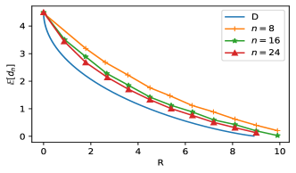
(a) Bernoulli, $m=10$

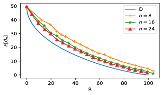
(b) Bernoulli, $m=100$

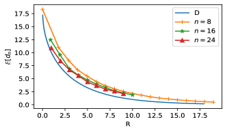
(c) Gaussian, $m=10$

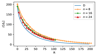
(d) Gaussian, $m=100$

Figure 10: Performance of Algorithm 1 and the distortion-rate functions of different probabilities.

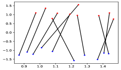
(a) $\boldsymbol{L}=\|x_{1}-x_{2}\|^{2}$

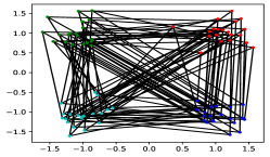
(b) $\boldsymbol{L}=\sum_{i=1}^{3}\|x_{i}-x_{i+1}\|^{2}$

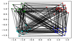
(c) $\boldsymbol{L}=\sum_{i\neq j}\|x_{i}-x_{j}\|^{2}$

Figure 11: Correspondence between the observations by MOT.

X Discussion and conclusions

In this paper, we present our causal model as the source coding side of a given multipartite correlation. It contains two conditions that ensure that its output statistics are nearly identical to the correlation and that it follows a causal order with no-signaling condition. Our approach involves classical information-theoretic methods such as Slepian-Wolf coding and covering lemma. These methods can be unified into a concept known as random binning, as also discussed in [26]. Random binning can be thought of as the extraction of randomness. Correlation is then established with the causal links that carry this randomness. Our results provide the physical meaning of several quantities and show consistency with previous works such as [22, 49, 26]. Notably, as the number of subsystems surpasses two, additional conditions become necessary in several of our results, i.e. Theorem 2, Proposition 2, and Proposition 9.

We include some further discussion. In Section VII, the concept of asymptotic equivalence arises from the nearly uniform property of secret keys [52]. This property is also known as information spectrum, a fundamental concept in information theory [76]. We note that the system we studied in Section VII bears a resemblance to the graphical lossy compression problem, and both problems make use of the covering lemma. The El Gamal–Cover inner bound using the multivariate covering lemma is also tight in several cases of multiple description problems [77]. Nevertheless, there are intrinsic differences between these two problems. In multiple description networks, the information spectrum is not considered on the receiver side. In our problem, the information spectrum is considered and new randomness can be generated on different marginals when establishing the joint key, according to Lemma 3. This leads to a major difference between our expression of the optimal rate and that of problems like multiple description network coding [78, 79]. Our problem further leads to a rate-distortion expression. We note that classical logarithmic information measures are closely related to physics (see, for example, the second law of thermodynamics in [75, Section 4.4]) and are continuous and convex (or concave) w.r.t. probability measures. Entropic OT, our rate-distortion expression, is also shown to be equivalent to another classical fluid dynamics problem called Schrödinger bridge [80]. The connection from our unicast traffic to the broadcast traffic in [24] is also intuitive. The broadcast rate is a variational form with $C(X_{1:m}|U):=C(X_{1:m}U)-mH(U)$. The broadcast signal with shared randomness can superpose another signal written as $\omega\oplus u$ and recover both of them, thus the unicast rate can remove $mH(U)$.

Appendix A Variations of secret key problem

A-A Secret key problem with time division

Let $X_{1:m}:=(X_{1:m,1},X_{1:m,2},\cdots,X_{1:m,T})$, where $X_{1:m,t}$ are mutually independent for $t\in\{1,\cdots,T\}$ and $T$ is the number of the time slots. Let the joint key $X^{n}_{1:m}:=(X^{n}_{1:m,1},X^{n}_{1:m,2},\cdots,X^{n}_{1:m,T})$ satisfying $\operatorname{TV}(P_{X^{n}_{1:m}},P_{X^{\otimes n}_{1:m}})<\epsilon$. Assume that $\mathcal{I}_{t}\subset\mathcal{M}$ is the set of the senders and $\mathcal{I}^{c}_{t}$ is the set of the receivers at each slot $t$. For $i\in\mathcal{I}_{t}$ and $j\in\mathcal{I}^{c}_{t}$, we denote $M_{i,j}$ as the message that $i$ sends to $j$. The receiver recovers its information $Y^{n}_{j}=g_{j}(M_{\mathcal{I}_{j},j},X^{n}_{j})\in\mathcal{Y}^{n}_{j}$ for all the possible distributions on $\mathcal{Y}^{n}_{j}$, where $X^{n}_{j}:=\{X^{n}_{j,t}|j\in\mathcal{I}^{c}_{t},\forall t\}$ and $\mathcal{I}_{j}:=\{i\in\mathcal{I}_{t}|j\in\mathcal{I}^{c}_{t},\forall t\}$. We assume $I(Y^{n}_{j};M_{\mathcal{I}_{j},j})\leq n\delta$ and $H(X_{j_{t}}|X_{\mathcal{I}_{t}})=0$. Let $R(\mathcal{Y}^{n}_{\mathcal{I}^{c}}):=\liminf_{n\rightarrow\infty}\frac{1}{n}\sum_{j\in\mathcal{M}}\log|\mathcal{Y}^{n}_{j}|$ be the rate of a sequence of alphabets. We define $R^{\prime}_{\text{rec}}(X_{1:m}):=\sup R(\mathcal{Y}^{n}_{\mathcal{I}^{c}})$ be the classical secrecy rate, where the supremum is among all the sequences of the alphabets and all $\mathcal{I}$ satisfying the given conditions of secure communication. We have the following corollary.

Corollary 3.

$$C(X_{1:m})\geq R^{\prime}_{\text{rec}}(X_{1:m}).$$ (109)

Proof.

Let $Y^{n}_{j}$ be uniform on $\mathcal{Y}^{n}_{j}$. The assumption $I(Y^{n}_{j};M_{\mathcal{I}_{j},j})\leq n\delta$ implies $H(Y^{n}_{j})-H(Y^{n}_{j}|M_{\mathcal{I}_{j},j})\leq n\delta$. Thus

$$\log|\mathcal{Y}^{n}_{j}|= H(Y^{n}_{j})$$

$$\leq H(Y^{n}_{j}|M_{\mathcal{I}_{j},j})+n\delta$$

$$\leq \sum_{t:j\in\mathcal{I}^{c}_{t}}H(X^{n}_{j,t})+n\delta,$$ (110)

where (110) is from data processing inequality. Then

$$\sum_{j\in\mathcal{M}}\log|\mathcal{Y}^{n}_{j}|\leq \sum_{j\in\mathcal{M}}\sum_{t:j\in\mathcal{I}^{c}_{t}}H(X^{n}_{j,t})+n\delta^{\prime}$$ (111)

$$= \sum_{t=1}^{T}\sum_{j_{t}\in\mathcal{I}^{c}_{t}}I(X^{n}_{j,t};X^{n}_{\mathcal{I}_{t}})+n\delta^{\prime\prime}$$ (112)

$$\leq \sum_{t=1}^{T}nC(X_{1:m,t})+n\delta^{\prime\prime\prime}$$ (113)

$$= nC(X_{1:m})+nT\delta^{\prime\prime\prime},$$

where (111) is from (110), (112) is from $H(X_{j_{t}}|X_{\mathcal{I}_{t}})=0$, and (113) is from Lemma 1. ∎

A-B Secret key problem with eavesdropping

Assume that $\mathcal{I}\subset\mathcal{M}$ is the set of the senders and $\mathcal{I}^{c}:=\mathcal{M}\backslash\mathcal{I}$ is the set of the receivers. Let $\Lambda(X^{n}_{1:m})$ be a distillation of key and let $\Lambda_{j}$ be the key owned by user $j$. For $i\in\mathcal{I}$ and $j\in\mathcal{I}^{c}$, we denote $M_{i,j}$ as the message that $i$ sends to $j$. The receiver recovers its information $Y^{n}_{j}=g_{j}(M_{\mathcal{I},j},\Lambda_{j})\in\mathcal{Y}^{n}_{j}$ for all the possible distributions on $\mathcal{Y}^{n}_{j}$, where $X^{n}_{j}$ is the $j$-th marginal of a correlation $X^{n}_{1:m}$ satisfying $\operatorname{TV}(P_{X^{n}_{1:m}Z^{n}},P^{\otimes n}_{X_{1:m}Z})<\epsilon$ with a given $X_{1:m}Z$. It satisfies that $I(Y^{n}_{j};M_{\mathcal{I},\mathcal{I}^{c}},Z^{n})\leq n\delta$ and $H(\Lambda_{j}|\Lambda_{\mathcal{I}})=0$, which means that the information leakage when the message is eavesdropped is almost zero, and the randomness of decryption is determined by the randomness of encryption. Let $R(\mathcal{Y}^{n}_{\mathcal{I}^{c}}):=\liminf_{n\rightarrow\infty}\frac{1}{n}\sum_{j\in\mathcal{I}^{c}}\log|\mathcal{Y}^{n}_{j}|$ be the rate of a sequence of alphabets. We define $R_{\text{rec}}(X_{1:m}|Z):=\sup R(\mathcal{Y}^{n}_{\mathcal{I}^{c}})$ be the classical secrecy rate, where the supremum is among all the sequences of the alphabets and all $\mathcal{I}$ satisfying the given conditions of secure communication. Then we have the next corollary.

Corollary 4.

$$C(X_{1:m}|Z)\geq R_{\text{rec}}(X_{1:m}|Z).$$ (114)

Proof.

Let $Y^{n}_{j}$ be uniform on $\mathcal{Y}^{n}_{j}$. The assumption $I(Y^{n}_{j};M_{\mathcal{I},\mathcal{I}^{c}},Z^{n})\leq n\delta$ implies $H(Y^{n}_{j})-H(Y^{n}_{j}|M_{\mathcal{I},\mathcal{I}^{c}},Z^{n})\leq n\delta$. Thus

$$\log|\mathcal{Y}^{n}_{j}|= H(Y^{n}_{j})$$

$$\leq H(Y^{n}_{j}|M_{\mathcal{I},\mathcal{I}^{c}},Z^{n})+n\delta$$

$$\leq H(\Lambda_{j}|Z^{n})+n\delta,$$ (115)

where (115) is from data processing inequality. Then

$$\sum_{j\in\mathcal{I}^{c}}\log|\mathcal{Y}^{n}_{j}|\leq \sum_{j\in\mathcal{I}^{c}}H(\Lambda_{j}|Z^{n})+n\delta^{\prime}$$ (116)

$$= \sum_{j\in\mathcal{I}^{c}}I(\Lambda_{j};\Lambda_{\mathcal{I}}|Z^{n})+n\delta^{\prime\prime}$$ (117)

$$\leq nC(X_{1:m}|Z)+n\delta^{\prime\prime\prime},$$ (118)

where (116) is from (115), (117) is from $H(\Lambda_{j}|\Lambda_{\mathcal{I}})=0$, and (118) is from Lemma 1 and the secrecy monotone of total correlation [22]. ∎

References

• [1] E. Chitambar and G. Gour, “Quantum resource theories,” Reviews of modern physics, vol. 91, no. 2, p. 025001, 2019.
• [2] A. Acín, J. I. Cirac, and L. Masanes, “Multipartite bound information exists and can be activated,” Physical review letters, vol. 92, no. 10, p. 107903, 2004.
• [3] O. Leskovjanová and L. Mišta Jr, “Classical analog of the quantum marginal problem,” Physical Review A, vol. 101, no. 3, p. 032341, 2020.
• [4] V. Scarani, H. Bechmann-Pasquinucci, N. J. Cerf, M. Dušek, N. Lütkenhaus, and M. Peev, “The security of practical quantum key distribution,” Reviews of modern physics, vol. 81, no. 3, p. 1301, 2009.
• [5] V. Scarani, N. Gisin, N. Brunner, L. Masanes, S. Pino, and A. Acín, “Secrecy extraction from no-signaling correlations,” Physical Review A, vol. 74, no. 4, p. 042339, 2006.
• [6] M. Christandl, A. Ekert, M. Horodecki, P. Horodecki, J. Oppenheim, and R. Renner, “Unifying classical and quantum key distillation,” in Theory of Cryptography: 4th Theory of Cryptography Conference, TCC 2007, Amsterdam, The Netherlands, February 21-24, 2007. Proceedings 4.   Springer, 2007, pp. 456–478.
• [7] R. Augusiak and P. Horodecki, “Multipartite secret key distillation and bound entanglement,” Physical Review A, vol. 80, no. 4, p. 042307, 2009.
• [8] R. Horodecki, P. Horodecki, M. Horodecki, and K. Horodecki, “Quantum entanglement,” Reviews of modern physics, vol. 81, no. 2, p. 865, 2009.
• [9] H. Buhrman, R. Cleve, S. Massar, and R. De Wolf, “Nonlocality and communication complexity,” Reviews of modern physics, vol. 82, no. 1, p. 665, 2010.
• [10] J. Barrett, N. Linden, S. Massar, S. Pironio, S. Popescu, and D. Roberts, “Nonlocal correlations as an information-theoretic resource,” Physical review A, vol. 71, no. 2, p. 022101, 2005.
• [11] L. Masanes, A. Acín, and N. Gisin, “General properties of nonsignaling theories,” Physical Review A, vol. 73, no. 1, p. 012112, 2006.
• [12] A. Acín and N. Gisin, “Quantum correlations and secret bits,” Physical review letters, vol. 94, no. 2, p. 020501, 2005.
• [13] A. K. Ekert, “Quantum cryptography based on bell’s theorem,” Phys. Rev. Lett., vol. 67, pp. 661–663, Aug 1991.
• [14] M. Hillery, V. Bužek, and A. Berthiaume, “Quantum secret sharing,” Physical Review A, vol. 59, no. 3, p. 1829, 1999.
• [15] M. Pivoluska, M. Huber, and M. Malik, “Layered quantum key distribution,” Physical Review A, vol. 97, no. 3, p. 032312, 2018.
• [16] F. Grasselli, H. Kampermann, and D. Bruß, “Finite-key effects in multipartite quantum key distribution protocols,” New Journal of Physics, vol. 20, no. 11, p. 113014, 2018.
• [17] M. Proietti, J. Ho, F. Grasselli, P. Barrow, M. Malik, and A. Fedrizzi, “Experimental quantum conference key agreement,” Science Advances, vol. 7, no. 23, p. eabe0395, 2021.
• [18] M. Epping, H. Kampermann, D. Bruß et al., “Multi-partite entanglement can speed up quantum key distribution in networks,” New Journal of Physics, vol. 19, no. 9, p. 093012, 2017.
• [19] S. Wengerowsky, S. K. Joshi, F. Steinlechner, H. Hübel, and R. Ursin, “An entanglement-based wavelength-multiplexed quantum communication network,” Nature, vol. 564, no. 7735, pp. 225–228, 2018.
• [20] S. K. Joshi, D. Aktas, S. Wengerowsky, M. Lončarić, S. P. Neumann, B. Liu, T. Scheidl, G. C. Lorenzo, Ž. Samec, L. Kling et al., “A trusted node–free eight-user metropolitan quantum communication network,” Science advances, vol. 6, no. 36, p. eaba0959, 2020.
• [21] C. E. Shannon, “A mathematical theory of communication,” The Bell system technical journal, vol. 27, no. 3, pp. 379–423, 1948.
• [22] N. J. Cerf, S. Massar, and S. Schneider, “Multipartite classical and quantum secrecy monotones,” Physical Review A, vol. 66, no. 4, p. 042309, 2002.
• [23] S. Watanabe, “Information theoretical analysis of multivariate correlation,” IBM Journal of research and development, vol. 4, no. 1, pp. 66–82, 1960.
• [24] G. R. Kurri, V. M. Prabhakaran, and A. D. Sarwate, “Coordination through shared randomness,” IEEE Transactions on Information Theory, vol. 67, no. 8, pp. 4948–4974, 2021.
• [25] A. El Gamal and Y.-H. Kim, Network information theory.   Cambridge University Press, 2011.
• [26] M. H. Yassaee, M. R. Aref, and A. Gohari, “Achievability proof via output statistics of random binning,” IEEE Transactions on Information Theory, vol. 60, no. 11, pp. 6760–6786, 2014.
• [27] M. Winczewski, T. Das, and K. Horodecki, “Limitations on a device-independent key secure against a nonsignaling adversary via squashed nonlocality,” Physical Review A, vol. 106, no. 5, p. 052612, 2022.
• [28] K. Horodecki, M. Winczewski, and S. Das, “Fundamental limitations on the device-independent quantum conference key agreement,” Physical Review A, vol. 105, no. 2, p. 022604, 2022.
• [29] A. Philip, E. Kaur, P. Bierhorst, and M. M. Wilde, “Multipartite intrinsic non-locality and device-independent conference key agreement,” Quantum, vol. 7, p. 898, 2023.
• [30] J. Pearl, Causality.   Cambridge University Press, 2009.
• [31] T. S. Han and S. Verdú, “Approximation theory of output statistics,” IEEE Transactions on Information Theory, vol. 39, no. 3, pp. 752–772, 1993.
• [32] P. W. Cuff, H. H. Permuter, and T. M. Cover, “Coordination capacity,” IEEE Transactions on Information Theory, vol. 56, no. 9, pp. 4181–4206, 2010.
• [33] P. Cuff, “Distributed channel synthesis,” IEEE Transactions on Information Theory, vol. 59, no. 11, pp. 7071–7096, 2013.
• [34] A. Winter, ““extrinsic”and “intrinsic”data in quantum measurements: Asymptotic convex decomposition of positive operator valued measures,” Communications in mathematical physics, vol. 244, pp. 157–185, 2004.
• [35] C. H. Bennett, I. Devetak, A. W. Harrow, P. W. Shor, and A. Winter, “The quantum reverse shannon theorem and resource tradeoffs for simulating quantum channels,” IEEE Transactions on Information Theory, vol. 60, no. 5, pp. 2926–2959, 2014.
• [36] M. M. Wilde, P. Hayden, F. Buscemi, and M.-H. Hsieh, “The information-theoretic costs of simulating quantum measurements,” Journal of Physics A: Mathematical and Theoretical, vol. 45, no. 45, p. 453001, 2012.
• [37] T. A. Atif, M. Heidari, and S. S. Pradhan, “Faithful simulation of distributed quantum measurements with applications in distributed rate-distortion theory,” IEEE Transactions on Information Theory, vol. 68, no. 2, pp. 1085–1118, 2021.
• [38] O. Oreshkov, F. Costa, and Č. Brukner, “Quantum correlations with no causal order,” Nature communications, vol. 3, no. 1, p. 1092, 2012.
• [39] K. Goswami, C. Giarmatzi, M. Kewming, F. Costa, C. Branciard, J. Romero, and A. G. White, “Indefinite causal order in a quantum switch,” Physical review letters, vol. 121, no. 9, p. 090503, 2018.
• [40] E.-E. Tselentis and A. Baumeler, “Admissible causal structures and correlations,” PRX Quantum, vol. 4, p. 040307, Oct 2023.
• [41] O. Oreshkov and C. Giarmatzi, “Causal and causally separable processes,” New Journal of Physics, vol. 18, no. 9, p. 093020, 2016.
• [42] A. A. Abbott, C. Giarmatzi, F. Costa, and C. Branciard, “Multipartite causal correlations: polytopes and inequalities,” Physical Review A, vol. 94, no. 3, p. 032131, 2016.
• [43] G. Rubino, L. A. Rozema, A. Feix, M. Araújo, J. M. Zeuner, L. M. Procopio, Č. Brukner, and P. Walther, “Experimental verification of an indefinite causal order,” Science advances, vol. 3, no. 3, p. e1602589, 2017.
• [44] C. Hitchcock and M. Rédei, “Reichenbach’s Common Cause Principle,” in The Stanford Encyclopedia of Philosophy, Summer 2021 ed., E. N. Zalta, Ed.   Metaphysics Research Lab, Stanford University, 2021.
• [45] G. Murta, F. Grasselli, H. Kampermann, and D. Bruß, “Quantum conference key agreement: A review,” Advanced Quantum Technologies, vol. 3, no. 11, p. 2000025, 2020.
• [46] L. Salvail, M. Peev, E. Diamanti, R. Alléaume, N. Lütkenhaus, and T. Länger, “Security of trusted repeater quantum key distribution networks,” Journal of Computer Security, vol. 18, no. 1, pp. 61–87, 2010.
• [47] D. M. Greenberger, M. A. Horne, and A. Zeilinger, “Going beyond bell’s theorem,” Bell’s theorem, quantum theory and conceptions of the universe, pp. 69–72, 1989.
• [48] R. W. Hamming, “Error detecting and error correcting codes,” The Bell system technical journal, vol. 29, no. 2, pp. 147–160, 1950.
• [49] B. Groisman, S. Popescu, and A. Winter, “Quantum, classical, and total amount of correlations in a quantum state,” Physical Review A, vol. 72, no. 3, p. 032317, 2005.
• [50] M. Fannes, “A continuity property of the entropy density for spin lattice systems,” Communications in Mathematical Physics, vol. 31, pp. 291–294, 1973.
• [51] D. Slepian and J. Wolf, “Noiseless coding of correlated information sources,” IEEE Transactions on information Theory, vol. 19, no. 4, pp. 471–480, 1973.
• [52] I. Csiszár and J. Körner, Information theory: coding theorems for discrete memoryless systems.   Cambridge University Press, 2011.
• [53] D. Yang, K. Horodecki, M. Horodecki, P. Horodecki, J. Oppenheim, and W. Song, “Squashed entanglement for multipartite states and entanglement measures based on the mixed convex roof,” IEEE Transactions on Information Theory, vol. 55, no. 7, pp. 3375–3387, 2009.
• [54] C. H. Bennett, H. J. Bernstein, S. Popescu, and B. Schumacher, “Concentrating partial entanglement by local operations,” Physical Review A, vol. 53, no. 4, p. 2046, 1996.
• [55] M. A. Nielsen and I. L. Chuang, “Quantum computation and quantum information,” Phys. Today, vol. 54, no. 2, p. 60, 2001.
• [56] D. Deutsch and P. Hayden, “Information flow in entangled quantum systems,” Proceedings of the Royal Society of London. Series A: Mathematical, Physical and Engineering Sciences, vol. 456, no. 1999, pp. 1759–1774, 2000.
• [57] B. Pass, “On the local structure of optimal measures in the multi-marginal optimal transportation problem,” Calculus of Variations and Partial Differential Equations, vol. 43, no. 3, pp. 529–536, 2012.
• [58] P. Dupuis and R. S. Ellis, A weak convergence approach to the theory of large deviations, ser. Wiley series in probability and statistics.   Hoboken: Wiley-Interscience, 2011.
• [59] J.-D. Benamou, G. Carlier, M. Cuturi, L. Nenna, and G. Peyré, “Iterative bregman projections for regularized transportation problems,” SIAM Journal on Scientific Computing, vol. 37, no. 2, pp. A1111–A1138, 2015.
• [60] L. M. Bregman, “The relaxation method of finding the common point of convex sets and its application to the solution of problems in convex programming,” USSR computational mathematics and mathematical physics, vol. 7, no. 3, pp. 200–217, 1967.
• [61] M. J. Wainwright, M. I. Jordan et al., “Graphical models, exponential families, and variational inference,” Foundations and Trends® in Machine Learning, vol. 1, no. 1–2, pp. 1–305, 2008.
• [62] S. Wang, P. A. Stavrou, and M. Skoglund, “Generalizations of talagrand inequality for sinkhorn distance using entropy power inequality,” Entropy, vol. 24, no. 2, p. 306, 2022.
• [63] I. Haasler, R. Singh, Q. Zhang, J. Karlsson, and Y. Chen, “Multi-marginal optimal transport and probabilistic graphical models,” IEEE Transactions on Information Theory, vol. 67, no. 7, pp. 4647–4668, 2021.
• [64] G. Wunder, A. Flinth, D. Becker, and B. Groß, “Mimicking dh key exchange over a full duplex wireless channel via bisparse blind deconvolution,” in 2023 6th International Conference on Advanced Communication Technologies and Networking (CommNet), 2023, pp. 1–8.
• [65] J. Csima, “Multidimensional stochastic matrices and patterns,” Journal of algebra, vol. 14, no. 2, pp. 194–202, 1970.
• [66] G. Birkhoff, “Tres observaciones sobre el algebra lineal,” Univ. Nac. Tucuman, Ser. A, vol. 5, pp. 147–154, 1946.
• [67] J. Von Neumann, “A certain zero-sum two-person game equivalent to the optimal assignment problem,” Contributions to the Theory of Games, vol. 2, no. 0, pp. 5–12, 1953.
• [68] M. D. Plummer and L. Lovász, Matching theory.   Elsevier, 1986.
• [69] G. Friesecke, “A simple counterexample to the monge ansatz in multimarginal optimal transport, convex geometry of the set of kantorovich plans, and the frenkel–kontorova model,” SIAM Journal on Mathematical Analysis, vol. 51, no. 6, pp. 4332–4355, 2019.
• [70] G. Monge, “Mémoire sur la théorie des déblais et des remblais,” Histoire de l’Académie Royale des Sciences de Paris, 1781.
• [71] L. V. Kantorovich, “On the translocation of masses,” in Dokl. Akad. Nauk. USSR (NS), vol. 37, 1942, pp. 199–201.
• [72] D. Fulkerson, Hitchcock transportation problem.   Rand Corporation, 1956.
• [73] Y. Bai, B. Schmitzer, M. Thorpe, and S. Kolouri, “Sliced optimal partial transport,” in Proceedings of the IEEE/CVF Conference on Computer Vision and Pattern Recognition, 2023, pp. 13 681–13 690.
• [74] P. Jouguet, S. Kunz-Jacques, A. Leverrier, P. Grangier, and E. Diamanti, “Experimental demonstration of long-distance continuous-variable quantum key distribution,” Nature photonics, vol. 7, no. 5, pp. 378–381, 2013.
• [75] T. M. Cover, Elements of information theory.   John Wiley & Sons, 1999.
• [76] T. HAN, “Information-spectrum methods in information theory,” Applications of Mathematics, 2003.
• [77] A. Gamal and T. Cover, “Achievable rates for multiple descriptions,” IEEE Transactions on Information Theory, vol. 28, no. 6, pp. 851–857, 1982.
• [78] H. Yamamoto, “Source coding theory for cascade and branching communication systems,” IEEE Transactions on Information Theory, vol. 27, no. 3, pp. 299–308, 1981.
• [79] ——, “Source coding theory for a triangular communication system,” IEEE Transactions on Information Theory, vol. 42, no. 3, pp. 848–853, 1996.
• [80] C. Léonard, “A survey of the schrödinger problem and some of its connections with optimal transport,” Discrete and Continuous Dynamical Systems, vol. 34, no. 4, p. 1533, 2014.