Localisation of Gamma Ray Bursts using AstroSat Mass Model

Abstract

The Cadmium Zinc Telluride Imager (CZTI) aboard AstroSat has good sensitivity to Gamma Ray Bursts (GRBs), with close to 600 detections including about 50 discoveries undetected by other missions. However, CZTI was not designed to be a GRB monitor and lacks localisation capabilities. We introduce a new method of localising GRBs using ‘shadows’ cast on the CZTI detector plane due to absorption and scattering by satellite components and instruments. Comparing the observed distribution of counts on the detector plane with simulated distributions with the AstroSat Mass Model, we can localise GRBs in the sky. Our localisation uncertainty is defined by a two-component model, with a narrow Gaussian component that has close to 50% probability of containing the source, and the remaining spread over a broader Gaussian component with an 11.3 times higher $\sigma$. The width ($\sigma$) of the Gaussian components scales inversely with source counts. We test this model by applying the method to GRBs with known positions and find good agreement between the model and observations. This new ability expands the utility of CZTI in the study of GRBs and other rapid high-energy transients.

1 Introduction

High-energy transients such as Gamma-Ray Bursts (GRBs), soft gamma repeaters (SGRs), X-ray counterparts to fast radio bursts (FRBs), and electromagnetic counterparts to gravitational waves (EMGW) are extraordinary physical phenomena linked to the activities of compact objects like neutron stars and black holes. Recent years have seen increased interest in the search for and study of these high-energy transients due to their association with cosmological sources (Mészáros et al., 2019). Among these phenomena, GRBs stand out as particularly intriguing transient events, releasing an astonishing amount of energy of the order of $10^{51}$ to $10^{54}$ erg (Piron, 2016). The initial prompt emission during a GRB occurs within a brief duration, typically ranging from a fraction of a second to a few minutes — or even thousands of seconds in the longest cases (Zhang, 2014; von Kienlin et al., 2020a; Lien et al., 2016). However, the brevity and uncertain positional information of these events make their study challenging.

GRBs have been a subject of study for several decades. To track the afterglow of GRBs, numerous ground-based telescope networks have been established, complementing space-based instruments that initially detect the prompt emission for initial localisation. Survey telescopes like Panoramic Survey Telescope and Rapid Response System (PAN-STARRS; Chambers et al., 2016) and the Zwicky Transient Facility (Bellm, 2014) diligently follow up on transients and relay transient alerts through Astronomers Telegram (Hložek, 2019). Additionally, global radio telescopes, including Very Long Baseline Interferometry (VLBI; Chandra, 2016; Mundell et al., 2010), conduct follow-up studies of these transients. By studying transients across different wavelength bands, a comprehensive understanding of the GRB emission mechanism can be achieved, aiding the development and refinement of theoretical models.

The detection of GRB 170817A — the gamma ray burst associated with the gravitational wave event GW170817 along with the gravitational wave detection by Laser Interferometer Gravitational-wave Observatory (LIGO) has given birth to multi-messenger astronomy (Abbott et al., 2017). The detection of this GRB by Fermi (Goldstein et al., 2017) coincident with the gravitational wave signal spurred a flurry of multi-wavelength observations that led to detailed characterisation of this event. While Fermi (Goldstein et al., 2017) and Integral (Savchenko et al., 2017) detected this burst, it was missed by Swift and AstroSat which were sensitive enough to detect it as it was occulted by the Earth (Evans et al., 2017; Kasliwal et al., 2017). The non-detection by CZTI despite the flux being above the detection threshold proved the Earth-occulted scenario and aided in narrowing down the source localisation by a factor of two (Kasliwal et al., 2017). Detection and localisation of high-energy bursts has at times changed the complete interpretation of an event. The discovery of GRB 170105A and its localisation were key in proving that the orphan afterglow ATLAS17aeu was associated with this GRB and not the binary black hole merger GW170104 (Bhalerao et al., 2017b). AstroSat-CZTI has been detecting a large number of bursts and can be used to measure the polarisation of bright bursts (Chattopadhyay et al., 2019, 2022). However, polarisation analysis requires the knowledge of the source position in the sky, failing which the analysis cannot be completed. Two examples of such bursts are GRB 200503A (Gupta et al., 2020a) and GRB 201009A (Gupta et al., 2020b). While they were also detected by other spacecraft like AGILE (Ursi et al., 2020a, b), Konus-Wind (Hurley, private communication), the sources were not well-localised by any of them. This has prevented us thus far from making two valuable additions to the rather small number of GRBs with measured polarisation.

Astronomical X-ray instruments employ various methods for source localisation. One approach involves projection-based localisation, where the number of counts observed by different detectors of the same instrument facing different directions is compared. This technique is used by missions such as Fermi-GBM (Connaughton et al., 2015), CGRO-BATSE (Meegan et al., 1992), GECAM (Xin-Ying et al., 2020), and the upcoming Daksha mission (Bhalerao et al., 2022a), providing localisations within a few degrees. Another method utilizes a coded aperture mask (CAM) to achieve enhanced localisation accuracy of the order of a few arc minutes. Instruments like Swift-BAT (Barthelmy et al., 2005), INTEGRAL (Mereghetti et al., 2004), and ECLAIRS onboard the SVOM mission (Triou et al., 2009) utilize CAM for GRB localisation, but this improved localisation typically comes at the cost of a limited field of view. Additionally, the interplanetary network (IPN) technique, involving data from different satellites (Hurley et al., 2013; Hurley, 2020), enables GRB localisation by leveraging the separation and arrival time of bursts on multiple satellites.

To localise GRBs with AstroSat-CZTI, earlier attempts have been made by using ray-trace simulations which is an analytical method calculating the shadow (i.e. the degree of absorption and transmission) cast by different components of CZTI on the detector, for photons of given energy and direction of incidence and predict the effective area of the same (Bhalerao et al., 2017b). However, this method ignores the absorption or scattering contributions of the rest of the satellite, and hence is rather limited in its accuracy and the fraction of the sky where it is applicable. Hence, to localise the GRBs we present a method that uses the shadow cast by other instruments, allowing us to determine the GRB location by comparing the observations with simulations obtained using the AstroSat Mass Model (Mate et al., 2021). In this paper, we present the localisation results obtained by analyzing a sample of GRBs detected by AstroSat-CZTI, using the AstroSat Mass Model to localise these GRBs and validate our results using localisation information from other instruments like Fermi, Swift or Interplanetary network (IPN).

This paper is structured in the following fashion: We briefly describe the AstroSat-CZTI instrument and the Mass Model in section §2. The framework for localising GRBs using the AstroSat Mass Model is discussed in section §3. The localisation results for our GRB sample and the calculation of uncertainty on the result are discussed in section §4. In section §5, we summarize our results and describe the impact of our results on future work.

2 Transients with AstroSat-CZTI

AstroSat is India’s first multi-wavelength mission that carries instruments covering the energy range from ultraviolet to high-energy X-rays (Singh et al., 2014). The five principal scientific payloads onboard AstroSat are: (i) a Soft X-ray Telescope (SXT), (ii) three Large Area Xenon Proportional Counters (LAXPCs), (iii) a Cadmium-Zinc-Telluride Imager (CZTI), (iv) an Ultra-Violet Imaging Telescope (UVIT) configured as two independent telescopes, and (v) a Scanning Sky Monitor (SSM). The CZTI instrument onboard AstroSat is a high-energy X-ray instrument providing wide-field coverage. CZTI contains 64 detectors with 256 pixels each, arranged in a square pattern to obtain nearly 1000 cm² geometric area (Bhalerao et al., 2017a). Collimators limit the primary field of view to approximately 4.6°, but these become increasingly transparent to radiation above 100 keV. This, combined with the 20–200 keV sensitive energy range makes CZTI an excellent all-sky detector for high-energy transients. CZTI was not designed as a GRB detection instrument, but over the years of its operation, it has proven very successful in detecting a large number of GRBs (Sharma et al., 2021). In the 7 years of its operation AstroSat has detected close to 600 GRBs. AstroSat has also proven very successful in measuring the polarisation of GRBs, having studied 20 GRBs so far (Chattopadhyay et al., 2022).

As AstroSat can detect off-axis GRBs but does not have localisation capability, it has thus far relied on other GRB detection instruments for localisation information. The localisation method presented here can overcome this hurdle.

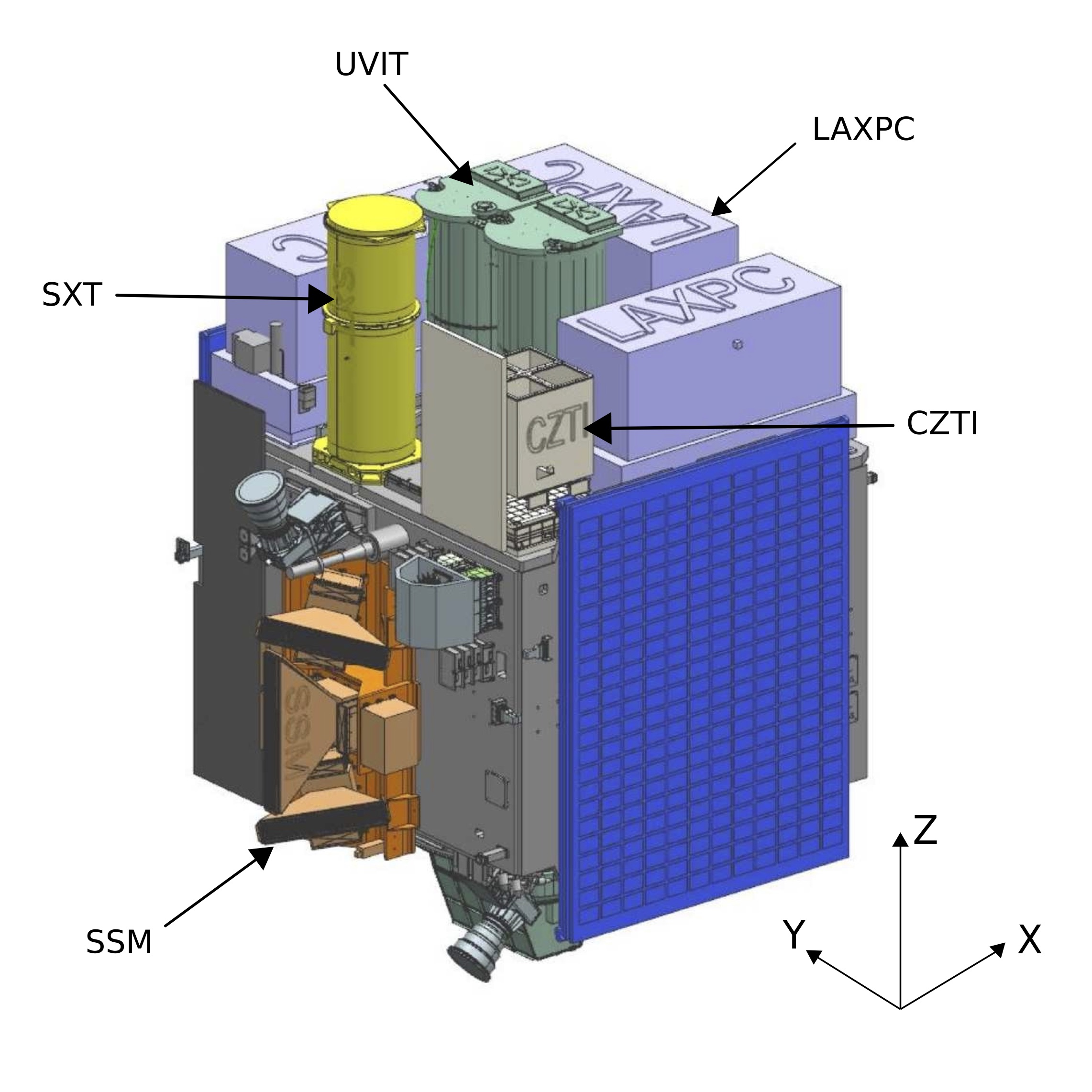
Figure 1: Representative CAD model of AstroSat with folded solar panels, featuring the five payloads of AstroSat, and displaying the coordinate axes for CZTI.

The AstroSat Mass Model is a numerical model of the satellite body, created using GEANT4 (Agostinelli et al., 2003), a tool for simulating interactions of photons and particles with matter. The details of AstroSat Mass Model can be found in Mate et al. (2021), hereafter referred to as MM21. We use the Mass Model to simulate the interaction of the incoming GRB photons with the satellite elements. Photons from a source incident on the satellite body may get transmitted, scattered, or absorbed and re-emitted with new energies and directions. All these effects lead to a direction-dependent ‘image’ on the detectors, which we term a ‘Detector Plane Histogram’ (DPH). Numerical calculations with the mass model can be used to simulate this DPH as a function of source direction. Thanks to the inhomogeneous distribution of satellite elements around the CZTI detectors, the DPH is different for each source direction. Thus, we can use the observed DPH for any GRB and compare it with a library of simulated DPHs to infer the location of the source in the sky. This principle is used to localise GRBs.

3 Localisation using Mass Model

In our localisation approach, we employ simulations generated by the AstroSat Mass Model at various positions in the sky. These simulations yield a DPH giving the expected number of photons in each of the 16,384 pixels of CZTI. This simulated DPH can then be compared with the observed background-subtracted DPH of a GRB. We bin the pixel data to perform a module-wise comparison between the observed data to the simulated DPH, as given by Equation 1:

$$\chi^{2}=\sum_{m=1}^{64}\frac{(N_{\mathrm{sim,m}}-N_{\mathrm{src,m}})^{2}}{\sigma_{sim,m}^{2}+\sigma_{src,m}^{2}}$$ (1)

where the summation is carried out over all 64 modules and on an average each module has more than 60 counts. The uncertainties in the simulated DPH are calculated as described in MM21. The GRB window $t_{\mathrm{src}}$ contains $N_{\mathrm{obs,m}}$ counts from the GRB as well as background. We calculate the source counts and uncertainty as follows:

$$N_{\mathrm{src,m}} = N_{\mathrm{obs,m}}-N_{\mathrm{bkg,m}}\times\frac{t_{\mathrm{src}}}{t_{\mathrm{bkg}}}$$ (2)

$$\sigma_{src,m}^{2} = N_{\mathrm{obs,m}}+N_{\mathrm{bkg,m}}\times\bigg{(}\frac{t_{\mathrm{src}}}{t_{\mathrm{bkg}}}\bigg{)}^{2}$$ (3)

The background $N_{\mathrm{bkg,m}}$ is measured using a longer window $t_{\mathrm{bkg}}$ and scaled before subtracting, in order to reduce the uncertainty contribution. The uncertainties in source and background are calculated assuming Poisson statistics. Repeating this procedure over the entire sky, the global minimum of $\chi^{2}$ gives the best-fit position of the source. As discussed in MM21, in practice it has been seen that there can be an overall scaling factor needed to make the GRB fluence match with the observed counts, and an offset factor to correct for any background subtraction residuals. Following MM21, we allow for additive and multiplicative scaling factors while calculating the $\chi^{2}$ values for each direction in our grid. As an example, Figure 2 shows the source DPH for GRB 190117A, compared with our simulated DPH for the closest grid point to the true GRB location on the sky.

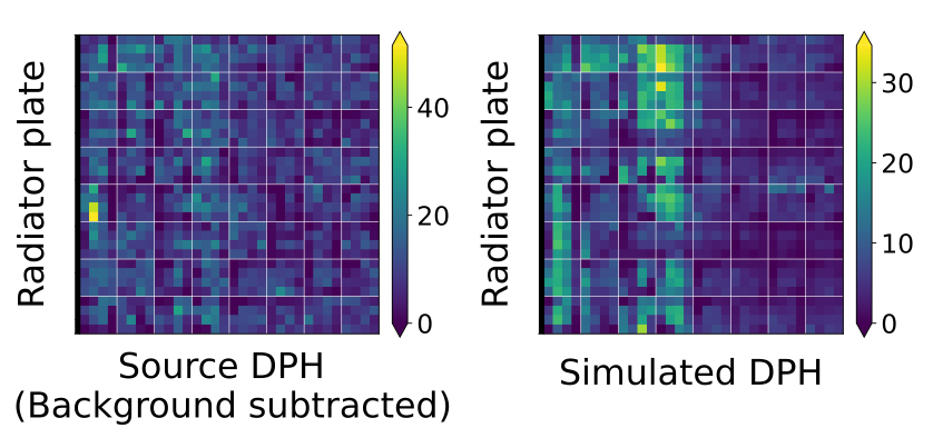
Figure 2: Comparing detector plane histograms (DPHs) for GRB 190117A. The left figure shows the observed background-subtracted DPH. The right side shows the scaled simulated DPH for a source located at the closest HTM grid point to the actual GRB position. The left image is more “grainy” due to the small number of statistics in observed data.

For localisation, we need simulations uniformly distributed over the entire sky. The selection of such points can be conveniently done using grids like the Hierarchical Triangular Mesh (HTM) (Kunszt et al., 2001) or Healpix (Gorski et al., 2005). For this work, HTM offers a distinct advantage: as we refine the resolution of HTM pixels, the centres of pixels from a coarse grid also become points on a finer grid. This allows us to refine our grid in selected parts of the sky without disrupting the grid pattern. Healpix, on the other hand, does not share this property. Hence, we opt to forgo the Healpix grid and instead pick an HTM grid of an appropriate resolution.

Based on simulations, we concluded that we need a grid resolution of $\sim 5^{\circ}$. This corresponds to a ‘Level 4’ HTM grid with pixel centres separated by $5.62^{\circ}$, having a total of 2048 pixels in the sky. We generated the Level 4 HTM grid in satellite $\theta$–$\phi$ coordinates, where $\theta$ is measured from the $Z$-axis and $\phi$ is measured from the $X$-axis along the $XY$ plane (Figure 1). We then undertook GEANT4 Mass Model simulations at each of those points. Since each GRB can have a different spectrum, we opted to simulate DPHs for monochromatic incident photons at 197 energies ranging from 20 keV – 2 MeV, with an adaptive step size based on energy resolution. The simulations commence at 20 keV, with increments of 5 keV up to 500 keV. In the range of 500 keV to 1 MeV, the step size is increased to 10 keV, followed by 20 keV steps in the 1 MeV to 2 MeV range. As discussed in MM21, photons up to about 2 MeV can make significant contributions in the 20–200 keV range. At each energy level, we simulate the interaction of $6.97$ million incident photons with the entire satellite. This simulation is carried out by employing a circular source plane with a radius of $200$ cm, resulting in a photon flux of $55.46$ photons cm^-2 as outlined in MM21. To carry out these simulations, we harnessed the high-performance computing cluster at IUCAA, Pune, leveraging 16 nodes, each equipped with 512 cores, which collectively accumulated to approximately $10^{5}$ CPU-hours.

The DPHs are then weighted by the spectrum of the incident GRB and summed to create the final simulated DPH for that direction. In cases where the GRB spectrum is unknown, we proceed with standard Fermi spectral parameters from Nava et al. (2011). Once the location is known, in principle, the mass model can be used to fit the GRB spectrum, which can be used iteratively to improve the location. Such iterative or joint fitting is beyond the scope of this work and will be addressed in a separate future work.

As an example, we show the $\chi^{2}$ contours for GRB 190117A in Figure 3. The best-fit position is then simply taken as the grid point having the lowest $\chi^{2}$ value. We note that the finite grid size means that even for the brightest GRB our $\theta$ offset will be as large as half of the grid size i.e. about $2.81^{\circ}$ or about the area of a pixel which is $20.14~{}\mathrm{deg}^{2}$.

4 Method

4.1 GRB sample

To validate our localisation results we select a sample of 29 bright GRBs detected by AstroSat before May 2023 and compare the results with the Mass Model simulations. The selection criterion for this sample is that the total GRB counts in the data should be $\geq 4000$ and the localisation information should be available from other missions like Fermi, Swift, Maxi, and IPN so that we can validate our localisation results. We converted the RA, and Dec obtained from these instruments to the $\theta-\phi$ coordinates in the CZTI frame. For these GRBs, the spectral parameters are obtained from either Fermi or Konus-Wind, and we scale the normalization values in the energy range from $70-200$ keV, which is the energy range in which we perform all our analyses for AstroSat-CZTI. One source we do not consider in our sample is GRB 160325A which was detected with 19229 counts. It was incident nearly on-axis for CZTI, where accurate localisation is done using the coded aperture mask (Vibhute et al., 2021). On the other hand, the Mass Model makes certain approximations which make it relatively less accurate for on-axis sources. Hence, we exclude this GRB from our sample.

4.2 Localisation contours

As discussed in §3, we calculate the $\chi^{2}$ for all directions for our GRB sample. We exclude the part of the sky that was occulted by the earth as seen from the satellite at the instant of the burst. Sample localisation contours are shown in Figure 3. The left column shows the contours plotted in RA-Dec coordinates, viewed from three different directions in the sky. The right column shows three views of contours plotted in $\theta$–$\phi$ coordinates. Where visible, the location of the GRB is marked with a cross.

Inspecting the contours created for our entire sample, we observe that in most of the cases, the source is well localised with contours showing a single global minimum, while in other cases there are multiple local minima with comparably low $\chi^{2}$ values. In some of these cases, the actual GRB location is closer to a secondary minimum rather than the global minimum. This suggests that we should select a “contour filling” method for describing the GRB location, rather than simply giving an angular offset.

For our 29-GRB sample, we have prior knowledge of the actual source location from other observational instruments. We approximate the GRB position with the HTM grid point closest to it. We denote the $\chi^{2}$ value at this grid position (cgp) by $\chi^{2}_{\mathrm{cgp}}$. Subsequently, we determine the number of grid points in our analysis that possess $\chi^{2}$ values less than $\chi^{2}_{\mathrm{cgp}}$. The total area with $\chi^{2}<\chi^{2}_{\mathrm{cgp}}$ is designated as the “enclosed area” $A_{e}$. In Table 2, we provide the obtained values of $A_{e}$ for each GRB in our dataset. Thus, the enclosed area $A_{e}$ is the smallest two-dimensional region, originating from regions with the highest likelihood, that encompasses the true source location.

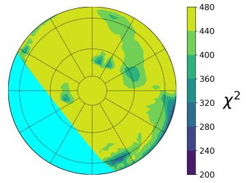
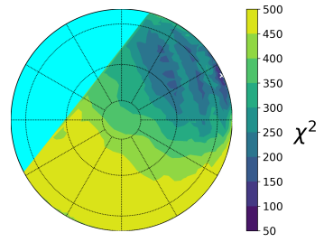
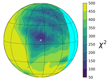
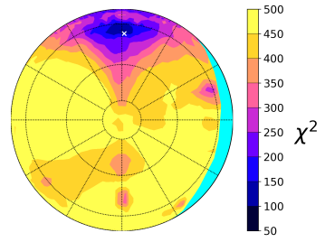
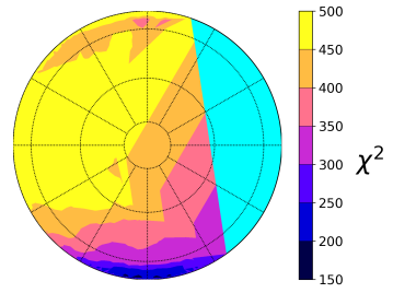
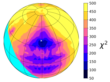
Figure 3: All-sky $\chi^{2}$ contour plots for GRB 190117A, as viewed from various directions in different coordinate systems. The top panel shows contour plots in the RA—Dec coordinate system, with the three figures showing views from RA, Dec = (0, $-90$), (0,90), and (113.86, 6.51) from left to right. The three figures in the bottom panel show contours in the satellite $\theta$—$\phi$ coordinates, as viewed from $\theta,\phi$ =(0, 0), (180, 0), and (51.26, 178.51) from left to right. The rightmost figure in each row is a view from the direction of the transient. The darkest region in the contour plot is the most likely location of the GRB from our fits. Where visible, the true location of the GRB is marked with a white cross.

4.3 Uncertainties in Localisation

Our localisation method is broadly similar to the source localisation by Fermi-GBM or by the proposed Daksha mission. In these cases, it is seen that the uncertainty in the localisation area scales inversely as the detected counts in GRBs detected by GBM (von Kienlin et al., 2020a) and simulations for Daksha (Bhalerao et al., 2022b). On the other hand, we can also treat the spacecraft elements as a coded aperture mask being used to obtain source positions. For coded aperture instruments, the localisation position uncertainty scales inversely as SNR (Baumgartner et al., 2013). For bright bursts that we discuss, SNR scales as $\sqrt{\mathrm{counts}}$, and again area uncertainty would scale inversely to the observed counts. Thus, we postulate that the localisation area will scale inversely with the observed counts as,

$$A_{50}=\frac{K_{a}}{\rm counts}$$ (4)

Where $K_{a}$ is a constant, and $A_{50}$ is defined as the area on the sky that has a 50% probability of enclosing the true location of the source.

If we had a large number of GRBs with the same counts then we could have created a distribution of the offsets and calculated $A_{50}$ as the median, thus giving us a value of $K_{a}$ from Equation 4. However, in practice our GRB sample has different counts for each source, and hence different values for $A_{50}$. To overcome this limitation, we measure the enclosed area $A_{e}$ for each GRB and normalise it by the expected $A_{50}$ for that source getting a new variable, the “normalised area” defined as $a=A_{e}/A_{50}$. The distribution of ‘$a$’ gives the probability distribution function of our uncertainties.

To evaluate this underlying probability distribution, we create a cumulative plot of the normalised area (Figure 4). For normally distributed uncertainties, this should yield an error function (erf). We can see that there is a sharply concentrated core of well-localised GRBs, but we also have a large number of outliers. We find that this is well modelled as a sum of two Gaussians: a narrow component and a broad component with standard deviations $\sigma_{1}$ and $\sigma_{2}$ respectively. The corresponding cumulative distribution function is given by Equation 5, where $f$ is the fractional contribution of the broad component.

$$cdf(a)=\int_{0}^{a}f\frac{1}{\sigma_{1}\sqrt{2\pi}}~{}e^{-x^{2}/2\sigma_{1}^{2}}+(1-f)\frac{1}{\sigma_{2}\sqrt{2\pi}}~{}e^{-x^{2}/2\sigma_{2}^{2}}dx$$ (5)

This distribution gives a good fit to observed data, with $\sigma_{1}=0.42$, $\sigma_{2}=4.76$ and $f=0.59$. We require that the median of this distribution occurs at $a=1$, yielding $K_{a}=6.87\times 10^{6}$. For these distributions, the enclosed probability for various values of $a$ is given in Table 1.

We investigated the GRBs to look for any patterns among GRBs that better line up with the narrow versus broad components of the distribution. We find that for GRBs above/below the detector plane ($\theta<60\degr$ or $\theta>90\degr$), the $\phi$ values are often correctly measured, and the discrepancy in $\theta$ can be large, even upto 60°. Additional minima are usually seen close to the detector plane ($60\degr<\theta<120\degr$), where the DPHs become relatively featureless. An illustration can be seen in Figure 3, where the lower right panel shows two broad local minima above and below the $\theta=90\degr$ detector plane. However, for this GRB the global minimum happens to be deeper than these spurious local minima, thus giving good localisation. On the other hand, for GRBs close to the detector plane ($60\degr<\theta<120\degr$), we find that the algorithm correctly places the GRBs within this $\theta$ range, but can have larger errors in both $\theta$ and $\phi$. This effect was also seen in MM21, the relatively featureless nature of the DPH resulted in poorer fits between simulations and observations. The effect can be mitigated to some extent if we know the coarse localisation of the GRBs from other sources — in which case we can focus only on the relevant local minimum, yielding better localisation. The details of this are not explored further in this work.

Table 1: Probability of contained area and corresponding normalised area.

Contained probability	Normalised area
0.10	0.12
0.20	0.24
0.30	0.39
0.40	0.59
0.50	1.00
0.60	1.98
0.70	3.16
0.80	4.56
0.90	6.55

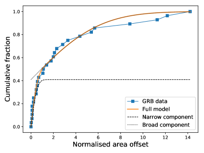
Figure 4: This figure presents the cumulative distribution of normalized area offsets for both GRB data and simulations. The data is modelled using a two-component model comprising a narrow and a broad component, with fitted values of $\sigma_{1}=0.42$, $\sigma_{2}=4.76$, and $f=0.59$, where $f$ represents the fractional contribution of the broad component.

5 Results and Discussions

Under the current counts cutoff criterion of $4000$ counts, we successfully localized $29$ GRBs within the dataset spanning a period of 7 years. The GRBs in our sample have minimum fluence $5.76\times 10^{-6}~{}\mathrm{erg~{}cm^{-2}~{}s^{-1}}$and maximum fluence $6.60\times 10^{-4}~{}\mathrm{erg~{}cm^{-2}~{}s^{-1}}$. Hence, we can localise GRBs with a minimum fluence of $\sim 6\times 10^{-6}~{}\mathrm{erg~{}cm^{-2}~{}s^{-1}}$ to an approximate area $A_{50}\approx$ 1700 sq. degree.

This method is now being used to localize bright GRBs detected by AstroSat-CZTI. As an illustrative case, consider the recent GRB 230817A detected by CZTI with 3083 counts, which we localized using our current method. The localisation obtained by Fermi for this GRB provided RA = $325.9$, Dec = $14.2$, and an uncertainty radius of $3.3^{\circ}$ (Fermi GBM Team, 2023). Our own localisation placed it at RA = $320.35$, Dec = $17.53$, with a corresponding enclosed area $A_{e}=201.43$ square degree. This is well within the expected uncertainty given by Equation 4, ${A_{50}}=2229.7$ square degree. The RA-Dec all-sky probability contour plot for this GRB is depicted in Figure 5.

Our preliminary tests have shown that this method extends well to the localisation of GRBs with fewer counts. This highlights the versatility of our approach, rendering it suitable for localizing GRBs detected by other instruments, particularly in situations where the satellite’s structural complexity presents challenges. Currently, this method is being employed to localize two specific GRBs, namely GRB 200503A and GRB 201009A, which will facilitate subsequent polarisation analysis of these events.

The integration of GRB localisation into the AstroSat-CZTI GRB pipelines is currently underway, and localisation for bright GRBs will be communicated through future announcements.

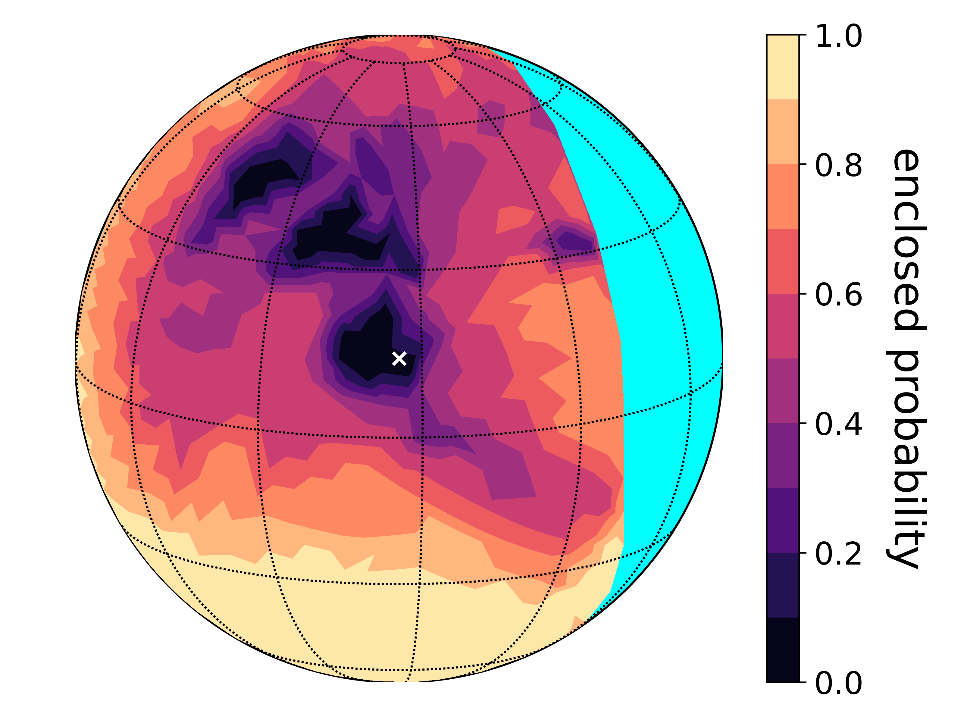
Figure 5: All-sky enclosed probability contour plot for GRB 230817A in RA, Dec; the white cross shows the actual position of the GRB. The cyan-coloured region is the region occulted by the earth.

Data Availability

The data underlying this article will be shared on reasonable request to the corresponding author.

References

- Abbott et al. (2017) Abbott B. P., et al., 2017, The Astrophysical Journal Letters, 848, L13
- Agostinelli et al. (2003) Agostinelli S., et al., 2003, Nuclear instruments and methods in physics research section A: Accelerators, Spectrometers, Detectors and Associated Equipment, 506, 250
- Barthelmy et al. (2005) Barthelmy S. D., et al., 2005, Space Science Reviews, 120, 143
- Baumgartner et al. (2013) Baumgartner W. H., Tueller J., Markwardt C. B., Skinner G. K., Barthelmy S., Mushotzky R. F., Evans P. A., Gehrels N., 2013, ApJS, 207, 19
- Beardmore et al. (2020) Beardmore A., et al., 2020, GRB Coordinates Network, 29061, 1
- Bellm (2014) Bellm E., 2014, in The Third Hot-wiring the Transient Universe Workshop.
- Bhalerao et al. (2017a) Bhalerao V., et al., 2017a, Journal of Astrophysics and Astronomy, 38, 1
- Bhalerao et al. (2017b) Bhalerao V., et al., 2017b, The Astrophysical Journal, 845, 152
- Bhalerao et al. (2022a) Bhalerao V., et al., 2022a, arXiv preprint arXiv:2211.12055
- Bhalerao et al. (2022b) Bhalerao V., et al., 2022b, arXiv e-prints, p. arXiv:2211.12055
- Biltzinger et al. (2019) Biltzinger B., Kunzweiler F., Berlato F., Burgess J., Greiner J., 2019, GRB Coordinates Network, 24677, 1
- Bissaldi (2016a) Bissaldi E., 2016a, GRB Coordinates Network, 19754, 1
- Bissaldi (2016b) Bissaldi E., 2016b, GRB Coordinates Network, 19754, 1
- Bissaldi (2018a) Bissaldi E., 2018a, GRB Coordinates Network, 22678, 1
- Bissaldi (2018b) Bissaldi E., 2018b, GRB Coordinates Network, 22678, 1
- Bissaldi & Fermi GBM Team (2021) Bissaldi E., Fermi GBM Team 2021, GRB Coordinates Network, 29393, 1
- Bissaldi & Fermi GBM Team (2022) Bissaldi E., Fermi GBM Team 2022, GRB Coordinates Network, 33034, 1
- Bissaldi & Meegan (2019) Bissaldi E., Meegan C., 2019, GRB Coordinates Network, 24692, 1
- Bissaldi et al. (2022) Bissaldi E., Meegan C., Fermi GBM Team 2022, GRB Coordinates Network, 31906, 1
- Blackburn (1995) Blackburn J. K., 1995, Astronomical Data Analysis Software and Systems IV, 77
- Chambers et al. (2016) Chambers K. C., et al., 2016, arXiv preprint arXiv:1612.05560
- Chandra (2016) Chandra P., 2016, Advances in Astronomy, 2016
- Chattopadhyay et al. (2019) Chattopadhyay T., et al., 2019, ApJ, 884, 123
- Chattopadhyay et al. (2022) Chattopadhyay T., et al., 2022, The Astrophysical Journal, 936, 12
- Connaughton et al. (2015) Connaughton V., et al., 2015, The Astrophysical Journal Supplement Series, 216, 32
- D’Ai et al. (2017) D’Ai A., et al., 2017, GRB Coordinates Network, 21989, 1
- D’Elia et al. (2018) D’Elia V., et al., 2018, GRB Coordinates Network, 23229, 1
- D’Elia et al. (2023) D’Elia V., et al., 2023, GRB Coordinates Network, 33285, 1
- Evans et al. (2017) Evans P. A., et al., 2017, Science, 358, 1565
- Fermi GBM Team (2019) Fermi GBM Team 2019, GRB Coordinates Network, 25240, 1
- Fermi GBM Team (2020) Fermi GBM Team 2020, GRB Coordinates Network, 27363, 1
- Fermi GBM Team (2021) Fermi GBM Team 2021, GRB Coordinates Network, 29232, 1
- Fermi GBM Team (2022a) Fermi GBM Team 2022a, GRB Coordinates Network, 31854, 1
- Fermi GBM Team (2022b) Fermi GBM Team 2022b, GRB Coordinates Network, 32820, 1
- Fermi GBM Team (2022c) Fermi GBM Team 2022c, GRB Coordinates Network, 33031, 1
- Fermi GBM Team (2023) Fermi GBM Team 2023, GRB Coordinates Network, 34464, 1
- Frederiks et al. (2016) Frederiks D., et al., 2016, GRB Coordinates Network, 19554, 1
- Frederiks et al. (2017) Frederiks D., et al., 2017, GRB Coordinates Network, 21166, 1
- Frederiks et al. (2019a) Frederiks D., et al., 2019a, GRB Coordinates Network, 23782, 1
- Frederiks et al. (2019b) Frederiks D., et al., 2019b, GRB Coordinates Network, 25868, 1
- Frederiks et al. (2021) Frederiks D., et al., 2021, GRB Coordinates Network, 30694, 1
- Gibson et al. (2018) Gibson S., et al., 2018, GRB Coordinates Network, 23097, 1
- Goldstein et al. (2017) Goldstein A., et al., 2017, The Astrophysical Journal Letters, 848, L14
- Gorski et al. (2005) Gorski K. M., Hivon E., Banday A. J., Wandelt B. D., Hansen F. K., Reinecke M., Bartelmann M., 2005, The Astrophysical Journal, 622, 759
- Gupta et al. (2020a) Gupta S., et al., 2020a, GRB Coordinates Network, 27680, 1
- Gupta et al. (2020b) Gupta S., Vibhute V. S. A., Bhattacharya D., Bhalerao V., Rao A., Vadawale S., Collaboration A. C., et al., 2020b, GRB Coordinates Network, 28589, 1
- Hamburg & Meegan (2017) Hamburg R., Meegan C., 2017, GRB Coordinates Network, 21839, 1
- Hamburg et al. (2017a) Hamburg R., Meegan C., Bissaldi E., Team F. G., et al., 2017a, GRB Coordinates Network, 21238, 1
- Hamburg et al. (2017b) Hamburg R., Meegan C., Bissaldi E., Fermi GBM Team 2017b, GRB Coordinates Network, 21238, 1
- Harris et al. (2020) Harris C. R., et al., 2020, Nature, 585, 357
- Hložek (2019) Hložek R., 2019, Publications of the Astronomical Society of the Pacific, 131, 118001
- Hui (2017a) Hui C., 2017a, GRB Coordinates Network, 22289, 1
- Hui (2017b) Hui C. M., 2017b, GRB Coordinates Network, 22289, 1
- Hunter (2007) Hunter J. D., 2007, Computing in Science & Engineering, 9, 90
- Hurley (2020) Hurley K. C., 2020, ApJ, 905, 82
- Hurley et al. (2013) Hurley K., et al., 2013, The Astrophysical Journal Supplement Series, 207, 39
- Hurley et al. (2019a) Hurley K., et al., 2019a, GRB Coordinates Network, 23764, 1
- Hurley et al. (2019b) Hurley K., et al., 2019b, GRB Coordinates Network, 25864, 1
- Kasliwal et al. (2017) Kasliwal M. M., et al., 2017, Science, 358, 1559
- Kunszt et al. (2001) Kunszt P. Z., Szalay A. S., Thakar A. R., 2001, in Mining the Sky: Proceedings of the MPA/ESO/MPE Workshop Held at Garching, Germany, July 31-August 4, 2000. pp 631–637
- Kunzweiler et al. (2020) Kunzweiler F., Biltzinger B., Berlato F., Greiner J., Burgess J., 2020, GRB Coordinates Network, 27546, 1
- Landsman (1993) Landsman W. B., 1993, Astronomical Data Analysis Software and Systems II, 52
- Lien et al. (2016) Lien A., et al., 2016, ApJ, 829, 7
- Liu et al. (2018) Liu Z., et al., 2018, GRB Coordinates Network, 23125, 1
- Mailyan et al. (2020) Mailyan B., Hamburg R., Fermi GBM Team 2020, GRB Coordinates Network, 27550, 1
- Malacaria et al. (2018) Malacaria C., Hamburg R., Meegan C., 2018, GRB Coordinates Network, 23095, 1
- Malacaria et al. (2020) Malacaria C., Veres P., Meegan C., Bissaldi E., Fermi GBM Team 2020, GRB Coordinates Network, 29073, 1
- Mate et al. (2021) Mate S., et al., 2021, Journal of Astrophysics and Astronomy, 42, 1
- Meegan et al. (1992) Meegan C., Fishman G., Wilson R., Paciesas W., Pendleton G., Horack J., Brock M., Kouveliotou C., 1992, Nature, 355, 143
- Mereghetti et al. (2004) Mereghetti S., Götz D., Borkowski J., 2004, Advances in Space Research, 34, 2729
- Mészáros et al. (2019) Mészáros P., Fox D. B., Hanna C., Murase K., 2019, Nature Reviews Physics, 1, 585
- Mingo et al. (2016) Mingo B., et al., 2016, GRB Coordinates Network, 19558, 1
- Mundell et al. (2010) Mundell C., Guidorzi C., Steele I., 2010, Advances in Astronomy, 2010
- Nava et al. (2011) Nava L., Ghirlanda G., Ghisellini G., Celotti A., 2011, A&A, 530, A21
- Page et al. (2021) Page K., Gropp J., Kuin N., Lien A., et al., 2021, GRB Coordinates Network, 30677, 1
- Piron (2016) Piron F., 2016, Comptes Rendus Physique, 17, 617
- Poolakkil & Meegan (2017) Poolakkil S., Meegan C., 2017, GRB Coordinates Network, 21992, 1
- Poolakkil et al. (2022) Poolakkil S., Meegan C., Fermi GBM Team 2022, GRB Coordinates Network, 32830, 1
- Poolakkil et al. (2023) Poolakkil S., Meegan C., Fermi GBM Team 2023, GRB Coordinates Network, 33288, 1
- Ridnaia et al. (2020) Ridnaia A., et al., 2020, GRB Coordinates Network, 27398, 1
- Roberts et al. (2019) Roberts O. J., Meegan C., Fermi GBM Team 2019, GRB Coordinates Network, 25248, 1
- Robitaille et al. (2013) Robitaille T. P., et al., 2013, Astronomy & Astrophysics, 558, A33
- Sakamaki et al. (2018) Sakamaki A., et al., 2018, GRB Coordinates Network, 23547, 1
- Savchenko et al. (2017) Savchenko V., et al., 2017, ApJ, 848, L15
- Sharma et al. (2021) Sharma Y., et al., 2021, Journal of Astrophysics and Astronomy, 42, 1
- Siegel et al. (2016) Siegel M., Barthelmy S., Lien A., Page K., Palmer D., 2016, GRB Coordinates Network, 19830, 1
- Siegel et al. (2017) Siegel M., et al., 2017, GRB Coordinates Network, 21821, 1
- Singh et al. (2014) Singh K. P., et al., 2014, in Space Telescopes and Instrumentation 2014: Ultraviolet to Gamma Ray. pp 517–531
- Stanbro & Meegan (2016) Stanbro M., Meegan C., 2016, GRB Coordinates Network, 19835, 1
- Stanbro et al. (2017) Stanbro M., Hui C., Meegan C., von Kienlin A., Team F. G., et al., 2017, GRB Coordinates Network, 21157, 1
- Svinkin et al. (2018) Svinkin D., et al., 2018, GRB Coordinates Network, 23128, 1
- Triou et al. (2009) Triou H., et al., 2009, in Hard X-Ray, Gamma-Ray, and Neutron Detector Physics XI. pp 169–177
- Tsvetkova et al. (2016) Tsvetkova A., et al., 2016, GRB Coordinates Network, 19511, 1
- Tsvetkova et al. (2018) Tsvetkova A., et al., 2018, GRB Coordinates Network, 23254, 1
- Ukwatta et al. (2016) Ukwatta T., Beardmore A., Evans P., Gehrels N., Kennea J., Krimm H., Page K., Palmer D., 2016, GRB Coordinates Network, 19502, 1
- Ursi et al. (2020a) Ursi A., et al., 2020a, GRB Coordinates Network, 27685, 1
- Ursi et al. (2020b) Ursi A., et al., 2020b, GRB Coordinates Network, 28588, 1
- Veres & Bissaldi (2018) Veres P., Bissaldi E., 2018, GRB Coordinates Network, 23548, 1
- Veres & Meegan (2016a) Veres P., Meegan C., 2016a, GRB Coordinates Network, 19901, 1
- Veres & Meegan (2016b) Veres P., Meegan C., 2016b, GRB Coordinates Network, 19901, 1
- Vibhute et al. (2021) Vibhute A., Bhattacharya D., Mithun N. P. S., Bhalerao V., Rao A. R., Vadawale S. V., 2021, Journal of Astrophysics and Astronomy, 42, 76
- Xin-Ying et al. (2020) Xin-Ying S., Wen-Xi P., Shuo X., Jin-Yuan L., Shao-Lin X., Qi L., Gang L., Yue Z., 2020, SCIENTIA SINICA Physica, Mechanica & Astronomica, 50, 129510
- Zhang (2014) Zhang B., 2014, International Journal of Modern Physics D, 23, 1430002
- von Kienlin et al. (2020a) von Kienlin A., et al., 2020a, ApJ, 893, 46
- von Kienlin et al. (2020b) von Kienlin A., et al., 2020b, ApJ, 893, 46