Continual Learning with Pre-Trained Models: A Survey

Abstract

Nowadays, real-world applications often face streaming data, which requires the learning system to absorb new knowledge as data evolves. Continual Learning (CL) aims to achieve this goal and meanwhile overcome the catastrophic forgetting of former knowledge when learning new ones. Typical CL methods build the model from scratch to grow with incoming data. However, the advent of the pre-trained model (PTM) era has sparked immense research interest, particularly in leveraging PTMs’ robust representational capabilities for CL. This paper presents a comprehensive survey of the latest advancements in PTM-based CL. We categorize existing methodologies into three distinct groups, providing a comparative analysis of their similarities, differences, and respective advantages and disadvantages. Additionally, we offer an empirical study contrasting various state-of-the-art methods to highlight concerns regarding fairness in comparisons. The source code to reproduce these evaluations is available at: https://github.com/sun-hailong/LAMDA-PILOT.

1 Introduction

With the rapid development of deep neuron networks, deep learning models have shown promising results in various applications He et al. (2016); Chao et al. (2020); Yang et al. (2015); Ye et al. (2021); Ning et al. (2022). However, the real-world scenario often presents data in a streaming format. Challenges such as privacy concerns Ning et al. (2023) and storage limitations prevent the permanent retention of the streaming data, necessitating a learning system capable of continuous adaptation and evolution, a process termed Continual Learning (CL) van de Ven et al. (2022); De Lange et al. (2021); Masana et al. (2023). A critical issue in CL is the phenomenon of catastrophic forgetting, where acquiring new knowledge leads to a significant decline in performance on previously learned tasks McCloskey and Cohen (1989). Numerous studies have been dedicated to addressing this issue within CL Gunasekara et al. (2023); Wang et al. (2023d, a, c); Zhuang et al. (2022); Zhao et al. (2021); Liu et al. (2024); Zhou et al. (2023b).

Traditionally, CL methods start with models that are “trained from scratch,” i.e., beginning with randomly initialized weights. However, the flourishing field of pre-training techniques has opened up new avenues. Utilizing pre-trained models (PTMs), which are developed from extensive datasets and sophisticated techniques Steiner et al. (2021), has shown great promise for CL. These PTMs inherently possess a strong generalizability for a variety of downstream tasks, making PTM-based CL an increasingly popular topic.

Figure 1 illustrates the distinctions between PTM-based and traditional continual learning approaches. Both methodologies employ the CL model within a data stream to adapt to a series of incoming tasks. The objective is for the model to assimilate new information while retaining previously acquired knowledge. This necessitates evaluating the model across all encountered tasks after each new task is learned. The primary divergence between PTM-based and traditional CL lies in the initial setup of the CL model. PTM-based strategies start with a large-scale pre-trained model, whereas traditional methods begin with a model trained from scratch. This difference can be analogized to human learning: traditional methods resemble training an infant to grow up and acquire new knowledge, while PTM-based methods are akin to leveraging the expertise of an adult for the same learning tasks.

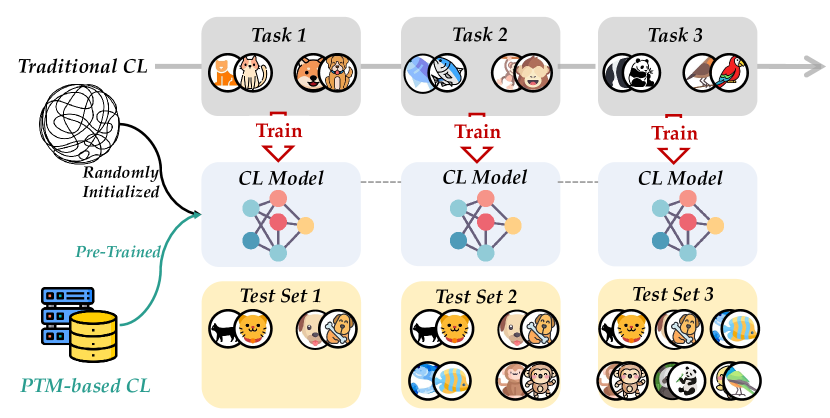
Figure 1: Illustrations of CL and its variations. New tasks arrive sequentially, and the model needs to learn them incrementally. After the learning process of each task, the model will be evaluated among all seen tasks. Traditional CL methods utilize randomly initialized weights as model initialization, while PTM-based methods make use of substantial and informative data to pre-train the CL model.

In this rapidly evolving field, existing surveys on CL primarily focus on typical algorithms that do not incorporate pre-trained models van de Ven et al. (2022); De Lange et al. (2021); Masana et al. (2023). Yet, in the current PTM era, PTM-based CL is emerging as a central area of interest. Observations suggest that the performance of PTM-based CL is approaching the upper bound of continual learning’s potential Zhou et al. (2023a), indicating a promising avenue for practical applications. Consequently, there is an immediate need for a comprehensive, current survey of PTM-based CL to further the advancement of the CL domain. Specific contributions of our survey are as follows:

1. We present the first comprehensive survey of recent advancements in pre-trained model-based continual learning, encompassing problem definitions, benchmark datasets, and evaluation protocols. Our systematic categorization of these methods into three subcategories based on their defining characteristics offers a thorough and structured overview of the subject.

2. Our evaluation extends to representative methods in each subcategory across seven benchmark datasets. In addition, we identify a critical factor that can affect the fairness of comparisons in PTM-based continual learning, providing insights into methodological assessments.

3. We highlight the current challenges and potential future directions in PTM-based continual learning. We intend to shed light on under-researched aspects to spur further investigations that will explore the various possible paths and their interrelations within this field.

2 Preliminaries

2.1 Continual Learning

Continual Learning De Lange et al. (2021) focuses on the learning scenario involving a sequence of tasks $\left\{\mathcal{D}^{1},\mathcal{D}^{2},\cdots,\mathcal{D}^{B}\right\}$. The $b$-th dataset $\mathcal{D}^{b}=\left\{\mathcal{X}_{b},\mathcal{Y}_{b}\right\}$ contains the set of input instances and their labels, i.e., $\mathcal{X}_{b}=\left\{{\bf x}_{i}\right\}_{i=1}^{n_{b}}$ and $\mathcal{Y}_{b}=\left\{y_{i}\right\}_{i=1}^{n_{b}}$. Among them, ${\bf x}_{i}\in\mathbb{R}^{D}$ is an instance of class $y_{i}\in Y_{b}$, $Y_{b}$ is the label space of task $b$. During the $b$-th training stage, we can only access data from $\mathcal{D}^{b}$. The goal of continual learning is to continually acquire the knowledge of all seen tasks, i.e., to fit a model $f({\bf x})$, and minimize the expected risk:

$$f^{*}=\underset{f\in\mathcal{H}}{\operatorname{argmin}}\enspace\mathbb{E}_{(\mathbf{x},y)\sim\mathcal{D}_{t}^{1}\cup\cdots\mathcal{D}_{t}^{b}}\mathbb{I}(y\neq f(\mathbf{x}))\,.$$ (1)

In Eq. 1, $\mathcal{H}$ is the hypothesis space, $\mathbb{I}(\cdot)$ is the indicator function which outputs $1$ if the expression holds and $0$ otherwise. $\mathcal{D}_{t}^{b}$ denotes the data distribution of task $b$. Hence, CL models are supposed to work well on all seen tasks, i.e., not only learning new tasks but also not forgetting former ones.

Variations of CL: There are many specific variations of continual learning based on the definitions of “tasks” van de Ven et al. (2022), e.g., Class-Incremental Learning (CIL), Task-Incremental Learning (TIL), and Domain-Incremental Learning (DIL). Specifically, in the training stage of CIL and TIL, we have $p(\mathcal{X}_{b})\neq p(\mathcal{X}_{b^{\prime}}),\mathcal{Y}_{b}\cap\mathcal{Y}_{b^{\prime}}=\varnothing$ for $b\neq b^{\prime}$. In other words, the new tasks contain new classes that have not been seen before, and the model is expected to learn new classes while not forgetting the former ones. However, the difference between them lies in the test stage, where TIL provides the task id (i.e., $b$) for the test instance while CIL does not. On the other hand, DIL focuses on the scenario where $p(\mathcal{X}_{b})\neq p(\mathcal{X}_{b^{\prime}}),\mathcal{Y}_{b}=\mathcal{Y}_{b^{\prime}}$ for $b\neq b^{\prime}$. For example, a new task contains images of the same class but with a domain shift, e.g., cartoon and oil painting.

2.2 Pre-Trained Models

Before the prosperity of PTMs, continual learning methods mainly resort to a residual network (i.e., ResNet He et al. (2016)) to serve as the backbone. However, recent years have witnessed the rapid development of transformer-base backbones Vaswani et al. (2017), and most PTM-based CL methods utilize an ImageNet21K Deng et al. (2009) pre-trained Vision Transformer (ViT) Dosovitskiy et al. (2020) as embedding function. Hence, we also focus on ViT as a representative PTM in this paper for its strong representation ability.

Specifically, in ViT, an input image is first divided into non-overlapping patches. These patches are then appended with a class token [CLS] and fed into an embedding layer followed by the vision transformer blocks. We denote the embedded patch features as ${\bf x}_{e}\in\mathbb{R}^{L\times d}$, where $L$ is the length of the sequence and $d$ is the embedding dim. In each vision transformer block, there are two main modules, i.e., a multi-head self-attention layer (MSA) and a two-layer MLP. The patch features are forwarded by $N$ cascaded transformer blocks, and we utilize the final [CLS] token as the feature for recognition. In the following discussions, we assume the availability of a pre-trained ViT on ImageNet as the initialization of $f({\bf x})$. We decompose the classification model into two parts: $f({\bf x})=W^{\top}\phi({\bf x})$, where $\phi(\cdot):\mathbb{R}^{D}\rightarrow\mathbb{R}^{d}$ is the embedding function (i.e., the embedded [CLS] token) and $W\in\mathbb{R}^{d\times|\bigcup_{b=1}^{B}{Y}_{b}|}$ is the classification head.

2.3 New Insights in Continual Learning Brought by Pre-Trained Models

Compared to training the embedding function from scratch, utilizing pre-trained models brings two major characteristics. Firstly, PTMs are born with “generalizability” compared to a randomly initialized model. From the representation learning perspective, the ultimate goal of continual learning is to learn a suitable embedding to capture all seen tasks, while PTMs provide a strong and generalizable feature extractor in the beginning. Hence, algorithms can be designed upon the frozen backbone in a non-continual manner Zhou et al. (2023c).

On the other hand, the structure of ViTs enables lightweight tuning with frozen pre-trained weights. Techniques like visual prompt tuning Jia et al. (2022) and adapter learning Chen et al. (2022) enable quick adaptation of PTMs to the downstream task while preserving generalizability. Hence, continual learning with PTMs shows stronger performance in resisting forgetting than training from scratch Cao et al. (2023).

3 Continual Learning with PTMs

We taxonomize current PTM-based CL studies into three categories based on their different ideas to tackle the learning problem, i.e., prompt-based methods, representation-based methods, and model mixture-based methods. These categories utilize different aspects of pre-trained models to facilitate continual learning. For example, given the strong generalization ability of PTMs, prompt-based methods resort to prompt tuning Jia et al. (2022) to exert lightweight updating of the PTM. Since the pre-trained weights are kept unchanged, the generalizability of PTMs can be preserved, and forgetting is thus alleviated. Similarly, representation-based methods directly utilize the generalizability of PTMs to construct the classifier. Lastly, model mixture-based methods design a set of models in the learning process and utilize model merging, model ensemble, and other mixture techniques to derive a final prediction. We show the taxonomy of PTM-based CL and list representative works in Figure 2. In the following section, we introduce each category and discuss their pros and cons in depth.

\begin{overpic}[width=433.62pt]{pics/tax} \put(5.0,24.0){\tiny{\cite[cite]{\@@bibref{Authors Phrase1YearPhrase2}{wang2022learning}{\@@citephrase{(}}{\@@citephrase{)}}}}} \put(5.0,20.5){\tiny{\cite[cite]{\@@bibref{Authors Phrase1YearPhrase2}{wang2022dualprompt}{\@@citephrase{(}}{\@@citephrase{)}}}}} \put(5.0,17.0){\tiny{\cite[cite]{\@@bibref{Authors Phrase1YearPhrase2}{wang2022s}{\@@citephrase{(}}{\@@citephrase{)}}}}} \put(5.0,13.5){\tiny{\cite[cite]{\@@bibref{Authors Phrase1YearPhrase2}{smith2023coda}{\@@citephrase{(}}{\@@citephrase{)}}}}} \put(5.0,10.0){\tiny{\cite[cite]{\@@bibref{Authors Phrase1YearPhrase2}{jung2023generating}{\@@citephrase{(}}{\@@citephrase{)}}}}} \put(5.0,6.5){\tiny{\cite[cite]{\@@bibref{Authors Phrase1YearPhrase2}{tang2023prompt}{\@@citephrase{(}}{\@@citephrase{)}}}}} \put(5.0,3.0){\tiny{\cite[cite]{\@@bibref{Authors Phrase1YearPhrase2}{khan2023introducing}{\@@citephrase{(}}{\@@citephrase{)}}}}} \par\par\put(39.0,24.0){\tiny{\cite[cite]{\@@bibref{Authors Phrase1YearPhrase2}{zhou2023revisiting}{\@@citephrase{(}}{\@@citephrase{)}}}}} \put(39.0,20.5){\tiny{\cite[cite]{\@@bibref{Authors Phrase1YearPhrase2}{janson2022simple}{\@@citephrase{(}}{\@@citephrase{)}}}}} \put(39.0,17.0){\tiny{\cite[cite]{\@@bibref{Authors Phrase1YearPhrase2}{mcdonnell2023ranpac}{\@@citephrase{(}}{\@@citephrase{)}}}}} \put(39.0,13.5){\tiny{\cite[cite]{\@@bibref{Authors Phrase1YearPhrase2}{ahrens2023read}{\@@citephrase{(}}{\@@citephrase{)}}}}} \put(39.0,10.0){\tiny{\cite[cite]{\@@bibref{Authors Phrase1YearPhrase2}{Zhang_2023_ICCV}{\@@citephrase{(}}{\@@citephrase{)}}}}} \put(39.0,6.5){\tiny{\cite[cite]{\@@bibref{Authors Phrase1YearPhrase2}{zheng2023learn}{\@@citephrase{(}}{\@@citephrase{)}}}}} \put(39.0,3.0){\tiny{\cite[cite]{\@@bibref{Authors Phrase1YearPhrase2}{guo2024federated}{\@@citephrase{(}}{\@@citephrase{)}}}}} \par\put(75.0,24.0){\tiny{\cite[cite]{\@@bibref{Authors Phrase1YearPhrase2}{Gao_2023_ICCV}{\@@citephrase{(}}{\@@citephrase{)}}}}} \put(75.0,20.5){\tiny{\cite[cite]{\@@bibref{Authors Phrase1YearPhrase2}{Zheng_2023_ICCV}{\@@citephrase{(}}{\@@citephrase{)}}}}} \put(75.0,17.0){\tiny{\cite[cite]{\@@bibref{Authors Phrase1YearPhrase2}{marouf2023weighted}{\@@citephrase{(}}{\@@citephrase{)}}}}} \put(75.0,13.5){\tiny{\cite[cite]{\@@bibref{Authors Phrase1YearPhrase2}{wang2023isolation}{\@@citephrase{(}}{\@@citephrase{)}}}}} \put(75.0,10.0){\tiny{\cite[cite]{\@@bibref{Authors Phrase1YearPhrase2}{chen2023promptfusion}{\@@citephrase{(}}{\@@citephrase{)}}}}} \put(75.0,6.5){\tiny{\cite[cite]{\@@bibref{Authors Phrase1YearPhrase2}{zhou2023learning}{\@@citephrase{(}}{\@@citephrase{)}}}}} \put(75.0,3.0){\tiny{\cite[cite]{\@@bibref{Authors Phrase1YearPhrase2}{wang2023hierarchical}{\@@citephrase{(}}{\@@citephrase{)}}}}} \par\par\end{overpic}

Figure 2: Taxonomy of PTM-based CL. We classify them into three subcategories, i.e., prompt-based ($\blacksquare$), representation-based ($\blacksquare$), and model mixture-based ($\blacksquare$). Different colors indicate different categories, and we list representative works in the boxes.

3.1 Prompt-based Methods

Observing the strong generalization ability of PTMs, how to tune the PTM leads to a trade-off — fully finetuning the weights to capture downstream tasks will erase the generalizable features, while fixing the backbone cannot encode downstream information into the backbone. To this end, visual prompt tuning (VPT) Jia et al. (2022) reveals a promising way to utilize lightweight trainable modules, e.g., prompts, to adjust the PTM. Specifically, it prepends a set of learnable parameters $P\in\mathbb{R}^{p\times d}$ (i.e., prompts) to the patch features ${\bf x}_{e}$. Hence, the model treats the concatenation of $[P,{\bf x}_{e}]$ as the input of the vision transformer blocks and minimizes the cross-entropy loss to encode task-specific information into these prompts with pre-trained weights frozen:

$$\min_{P\cup W}\sum_{({\bf x},y)\in\mathcal{D}^{b}}\ell\left(W^{\top}\phi\left({\bf x};P\right),y\right)\,,$$ (2)

where $\phi\left({\bf x};P\right)$ represents the prompted features by prepending the prompts. Optimizing Eq. 2 enables the model to encode task-specific information (i.e., the crucial features for $\mathcal{D}^{b}$) into the prompts. Hence, many works are designed to utilize prompt tuning for CL.

Prompt Pool: Although Eq. 2 enables the lightweight tuning of a pre-trained model, sequentially optimizing a single prompt with new tasks will suffer catastrophic forgetting, i.e., overwriting the prompt weights of former tasks leads to the incompatible representations between former tasks and latter ones. Hence, many works Wang et al. (2022c, b); Smith et al. (2023) propose to design the prompt pool, which collects a set of prompts, i.e., $\mathbf{P}=\{P_{1},P_{2},\cdots,P_{M}\}$, where $M$ is the size of the pool. The prompt pool can be seen as the external memory of the CL model, enabling instance-specific prompting during training and inference. Hence, the forgetting of a single prompt can be alleviated, while it requires a proper prompt selection mechanism.

Prompt Selection: With a set of prompts, we need to decide which prompt(s) to use for the specific instance, i.e., to define a retrieval function $g({\bf x})$ that selects instance-specific prompts. Prompt retrieval becomes the core problem in prompt-based methods, and many works design different variations. L2P Wang et al. (2022c) designs a key-query matching strategy, which assigns a learnable key $\mathbf{k}\in\mathbb{R}^{d}$ to each prompt. In this case, the prompt pool is formulated as $\mathbf{P}=\{(\mathbf{k}_{1},P_{1}),(\mathbf{k}_{2},P_{2}),\cdots,(\mathbf{k}_{M},P_{M})\}$. To retrieve instance-specific prompts, it utilizes a PTM without prompting (i.e., $\phi(\cdot)$) to encode the features into the key’s embedding space and select prompts with similar keys:

$$\mathbf{K}_{{\bf x}}=\underset{\left\{s_{i}\right\}_{i=1}^{N}\subseteq[1,M]}{\operatorname{argmin}}\sum_{i=1}^{N}\gamma\left(\phi({{\bf x}}),\mathbf{k}_{s_{i}}\right)\,,$$ (3)

where $\left\{s_{i}\right\}_{i=1}^{N}$ is the selected index set and $\mathbf{K}_{{\bf x}}$ is the selected top-N keys. $\gamma(\cdot,\cdot)$ denotes the cosine distance. Eq. 3 selects the most similar keys to the query instance, and the model optimizes the corresponding values (i.e., prompts) during the learning process:

$$\min_{\mathbf{K}\cup\mathbf{P}\cup W}\sum_{({\bf x},y)\in\mathcal{D}^{b}}\ell\left(W^{\top}\phi\left({\bf x};\mathbf{P}_{\bf x}\right),y\right)+\lambda\sum_{\mathbf{K}_{{\bf x}}}\gamma\left(\phi({\bf x}),\mathbf{k}_{s_{i}}\right)\,.$$ (4)

Hence, optimizing Eq. 4 also forces the keys to be similar to the encoded features. The above query-key matching process is an Expectation-Maximization (EM) procedure Moon (1996); Yadav et al. (2023). Specifically, in the E-step, the top-N keys are selected based on their similarity to the query feature. In the M-step, the keys are then pulled closer to the query.

Motivated by L2P, many works are proposed to improve the selection process. DualPrompt Wang et al. (2022b) explores the significance of prompt depth by attaching prompts to different layers. It also decouples the prompts into general and expert ones. Among them, general prompts are designed to encode the task-generic information, which is shared among all tasks. By contrast, expert prompts are task-specific, and the number is equal to that of tasks. It utilizes the same retrieval strategy in Eq. 3 during inference. PP-TF Yadav et al. (2023) applies a similar strategy in code generation models. S-Prompt Wang et al. (2022a) also considers a task-specific prompt strategy, which expands the prompt pool with a new prompt when learning a new task. Instead of key-query matching, it builds the task centers by conducting K-means clustering in every task and utilizes a KNN search to find the most similar task to get the prompt. MoP-CLIP Nicolas et al. (2024) extends S-Prompt by combining multiple prompts during inference.

Prompt Combination: While selecting prompts from the prompt pool sounds reasonable, the matching process in Eq. 3 is still a hard matching that can reproduce limited choices. Correspondingly, CODA-PromptSmith et al. (2023) suggests building an attention-based prompt from the prompt pool. During prompt retrieval, it utilizes the query feature $\phi({\bf x})$ to calculate an attention vector to all keys and utilize the attention results to create a weighted summation over the prompt components:

$$\textstyle P=\sum_{m=1}^{M}\gamma(\phi({\bf x})\odot\mathbf{a}_{m},\mathbf{k}_{m})P_{m}\,,$$ (5)

where $\mathbf{a}_{m}\in\mathbb{R}^{d}$ is the learnable attention vectors of the corresponding prompt, and $\odot$ denotes Hadamard product. Eq. 5 calculates the attention score between the input feature and the prompt keys via element-wise multiplication. Hence, if the query instance is more similar to a key vector, the corresponding prompt value will play a more important role in the final constructed prompt. Since it treats the prompts like ‘bases’ in the prompt space, it also designs an extra orthogonality loss to enhance prompt diversity.

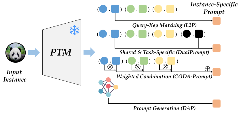
Figure 3: Different kinds of prompt selection, including key-value matching, shared and task-specific retrieval, attention-based combination, and instance-specific prompt generation.

Prompt Generation: While CODA-Prompt addresses the attention-based prompt combination, the combination process is still restricted by the prompt pool. Hence, many works move further to design meta-networks that can generate instance-specific prompts. Correspondingly, DAP Jung et al. (2023) achieves this goal by encoding prompt generation into an MLP network. It generates instance-specific prompts via:

$$P=\left(\gamma_{e}\operatorname{MLP}\left(\operatorname{LN}(\phi({\bf x}))^{\top}\right)+\beta_{e}\right)^{\top}\,,$$ (6)

where LN denotes layer normalization, $\gamma_{e}$, and $\beta_{e}$ are produced by linear transformations of the task prediction, serving as the weight and bias in prompt generation. Unlike the input-level prompt generation in Eq. 6, APG Tang et al. (2023) utilizes the attention mechanism for prompt generation at the middle layers of ViT.

Summary of Prompt-based Methods: We summarize the way of prompt selection in Figure 3, including the way of prompt retrieval in L2P, task-specific and general prompts in DualPrompt, attention-based combination in CODA-Prompt and prompt generation in DAP. Instead of selecting prompts, several works Liu et al. (2022); Razdaibiedina et al. (2023) also consider appending all prompts to the query instance or learning visual prompts (i.e., pixel-level parameters) Liu et al. (2023); Gan et al. (2023). Apart from the single visual modality, the model can also utilize textual information Radford et al. (2021) in learning and selecting suitable prompts with pre-trained vision-language models Khan et al. (2023); Villa et al. (2023); Wang et al. (2023e); Khattak et al. (2023).

Pros & Cons: Prompt-based methods strike a balance between pre-trained knowledge and downstream tasks with lightweight prompts, yielding many advantages. Firstly, prompts help bridge the domain gap and effectively encode task-specific knowledge. Secondly, since these lightweight modules have the same dimension as the features, saving prompts is parameter-efficient, which is naturally suitable for some edge scenarios like federated learning Guo et al. (2024). Lastly, learning the prompt pool acts as the external memory of the PTM, enabling adaptive knowledge retrieval and instance-specific prediction.

However, there are also some drawbacks. Firstly, some works Moon et al. (2023) find the prompt selection process in Eq. 3 converges to a single point, making the prompt selection only concentrate on the specific subset. Besides, since the keys and prompt values keep changing throughout the learning process, the updating of these parameters will erase that of former tasks. This further leads to matching-level and prompt-level forgetting, making the prompt selection process become the bottleneck in continual learning. Furthermore, if we use a fixed-size prompt pool, the representation ability will be restricted. By contrast, if the prompt pool grows as data evolves, it will result in a mismatch between training and testing since new prompts may be retrieved for old tasks. Lastly, although prompt-based methods reveal a promising solution for PTM-based CL, some works Zhou et al. (2023c) find their performance lower than a simple prototype-based baseline (as discussed in Section 3.2). While some prompt-based methods Jung et al. (2023) show surprising results, there are some concerns about the comparison fairness due to the batch-wise prompt section (as discussed in Section 4).

3.2 Representation-based Methods

Observing the strong representation ability of PTMs, one may wonder if they have already mastered the knowledge to classify new tasks. In other words, how can we measure the inherent ability of PTMs on these downstream tasks? Borrowing the idea from representation learning Ye et al. (2017), SimpleCIL Zhou et al. (2023c) suggests a simple way to achieve this goal. Facing the continual data stream, it freezes the pre-trained weights and extracts the center ${\bm{c}}$ (i.e., prototype) of each class:

$$\textstyle{\bm{c}}_{i}=\frac{1}{K}{\sum_{j=1}^{|\mathcal{{D}}^{b}|}\mathbb{I}(y_{j}=i)\phi({\bf x}_{j})}\,,$$ (7)

where $K={\sum_{j=1}^{|\mathcal{{D}}^{b}|}\mathbb{I}(y_{j}=i)}$. In Eq. 7, the embeddings of the same class are averaged, leading to the most common pattern of the corresponding class. Hence, it can serve as the ‘classification criterion’ or ‘template’ van de Ven et al. (2022) during inference. Correspondingly, SimpleCIL directly replaces the classifier weight of the $i$-th class with prototype (${\bm{w}}_{i}={\bm{c}}_{i}$), and utilize a cosine classifier for classification, i.e., $f(\mathbf{x})=\frac{W^{\top}\phi({\bf x})}{\|W\|_{2}\|\phi({\bf x})\|_{2}}$. Hence, facing a new task, we can calculate and replace the classifier for each class with the embedding frozen. Surprisingly, this simple solution shows superior performance than many prompt-based methods, e.g., L2P and DualPrompt. It indicates that PTMs already possess generalizable representations, which can be directly utilized for downstream tasks. A similar phenomenon has also been found in Janson et al. (2022), and Zheng et al. (2023a) applies it to large language models.

Concatenating Backbones: Observing the strong generalizability of PTMs, ADAM Zhou et al. (2023c) moves a step further by comparing the performance of new classes between the prototype-based classifier and fully-finetuned model. Surprisingly, it finds PTMs can achieve better performance on new classes if adapted to the downstream tasks. It indicates that PTMs, although generalizable, do not possess the task-specific information for the downstream data. Hence, ADAM suggests finetuning the PTM with parameter-efficient modules (e.g., prompts Jia et al. (2022) or adapters Chen et al. (2022)) and concatenating features of the pre-trained and adapted models:

$$\textstyle{\bm{c}}_{i}=\frac{1}{K}{\sum_{j=1}^{|\mathcal{{D}}^{b}|}\mathbb{I}(y_{j}=i)[\phi({\bf x}_{j}),\phi({\bf x}_{j};\text{PEFT})]}\,,$$ (8)

where $\phi({\bf x}_{j};\text{PEFT})$ indicates the finetuned model. In Eq. 8, the adaptation process bridges the domain gap between pre-trained and downstream datasets, and the concatenated features possess generalized (i.e., PTM) and task-specific (i.e., finetuned model) information. Hence, ADAM further improves the performance compared to SimpleCIL.

Utilizing Random Projection: Based on ADAM, RanPAC McDonnell et al. (2023) further finds that prototypes calculated by Eq. 8 often correlate between classes. Hence, it suggests using an online LDA classifier to remove class-wise correlations for better separability. Furthermore, to make the feature distribution for a Gaussian fit, it designs an extra random projection layer $\text{Proj}(\cdot):\mathbb{R}^{d}\rightarrow\mathbb{R}^{K},K\gg d$ to project features into the high dimensional space. Afterward, prototypes in the projected space are calculated, i.e., ${\bm{c}}_{i}=\frac{1}{K}{\sum_{j=1}^{|\mathcal{{D}}^{b}|}\mathbb{I}(y_{j}=i)\text{Proj}(\phi({\bf x}_{j};\text{PEFT})})$. Moreover, LayUP Ahrens et al. (2023) further finds the strong representation ability also lies in other deep layers of the transformer block. It treats the concatenation of the last $k$ layer features as the representation and trains an online LDA based on it.

Slow Learner with Feature Replay: In Eq. 8, the model’s generalizability and adaptivity are maintained by backbone concatenation. By contrast, there are also works aiming for the intersection between pre-trained and fully-adapted models. SLCA Zhang et al. (2023) suggests tuning the embedding function $\phi$ with a small learning rate while tuning the classifier $W$ with a large learning rate. This enables a gradual fitting of the features and quick adaptation of the classifiers. To resist forgetting former classifiers, it follows Zhu et al. (2021) to model class-wise feature distributions and replay them to calibrate the classifier.

Pros & Cons: Representation-based methods aim to take full advantage of the pre-trained features, which show competitive performance in various tasks. This line of work has many advantages. Firstly, since class prototypes represent the most common pattern of the corresponding class, building recognition models with them is intuitive and interpretable. Utilizing a prototype-based classifier also provides a simple yet effective way to investigate the ‘baseline’ of PTM-based CL. Furthermore, this line of work mainly freezes the backbone and updates the classifier weight. The lightweight update cost makes them feasible in real-world applications, e.g., Guo et al. (2024) applies similar tricks to federated learning by synchronizing global prototypes in various clients.

However, there are also some drawbacks. Firstly, concatenating features from different models to formulate the class prototype ignores the redundancy across models. For example, the shared features could be extracted repeatedly in different backbones without a pruning strategy. Secondly, when the downstream task involves multiple domains, adapting the model within the first stage (as in Eq. 8) is insufficient to bridge the domain gap across datasets. In that case, continually adjusting the backbone could be more suitable to extract task-specific features.

3.3 Model Mixture-based Methods

The challenge of continual learning has been alleviated with the help of PTMs, enabling CL algorithms to start from a provident starting point. Hence, adapting PTMs to downstream tasks becomes simple, while preventing forgetting in the adaptation process requires more attention. To this end, model mixture-based methods aim to create a set of models during the continual learning process and conduct model ensemble or model merge during inference. Since information from multiple stages is mixed for the final prediction, catastrophic forgetting can be thus alleviated.

Model Ensemble: Since PTMs show generalizable features, creating a set of models based on the PTM becomes possible. ESN Wang et al. (2023g) creates a set of classifiers individually based on the same PTM during the learning process, i.e., it initializes and trains a new classifier head when facing a new task. During inference, it designs a voting strategy for these classifier heads by adopting a set of temperatures. LAE Gao et al. (2023) adopts a similar inference strategy by choosing the max logit across different models.

Since the core factor in an ensemble depends on the variance of learners, several works aim to enhance the diversity among models instead of building a set of classifiers with the same PTM. PromptFusion Chen et al. (2023) utilizes a pre-trained ViT and a CLIP Radford et al. (2021) and dynamically combines the logits during inference, i.e., $f({\bf x})=\lambda f_{\text{ViT}}({\bf x})+(1-\lambda)f_{\text{CLIP}}({\bf x})$. Different from the ensemble of multiple backbones, PROOF Zhou et al. (2023d) designs a more comprehensive inference format with only a single CLIP. Since CLIP enables cross-modal matching for visual and textual features, PROOF designs a three-level ensemble considering image-to-text, image-to-image prototype, and image-to-adjusted text with cross-modal fusion.

Table 1: Average and last continual learning performance on seven datasets. ‘IN-R/A’ stands for ‘ImageNet-R/A,’ ‘ObjNet’ stands for ‘ObjectNet,’ and ‘OmniBench’ stands for ‘OmniBenchmark.’ Different colors ($\blacksquare$ $\blacksquare$ $\blacksquare$) indicate different categories of methods. ‘DAP w/o BI’ indicates DAP without batch information.

Method	CIFAR B0 Inc5		CUB B0 Inc10		IN-R B0 Inc5		IN-A B0 Inc20		ObjNet B0 Inc10		OmniBench B0 Inc30		VTAB B0 Inc10
	$\bar{\mathcal{A}}$	${\mathcal{A}_{B}}$	$\bar{\mathcal{A}}$	${\mathcal{A}_{B}}$	$\bar{\mathcal{A}}$	${\mathcal{A}_{B}}$	$\bar{\mathcal{A}}$	${\mathcal{A}_{B}}$	$\bar{\mathcal{A}}$	${\mathcal{A}_{B}}$	$\bar{\mathcal{A}}$	${\mathcal{A}_{B}}$	$\bar{\mathcal{A}}$	${\mathcal{A}_{B}}$
L2P	85.94	79.93	67.05	56.25	66.53	59.22	49.39	41.71	63.78	52.19	73.36	64.69	77.11	77.10
DualPrompt	87.87	81.15	77.47	66.54	63.31	55.22	53.71	41.67	59.27	49.33	73.92	65.52	83.36	81.23
CODA-Prompt	89.11	81.96	84.00	73.37	64.42	55.08	53.54	42.73	66.07	53.29	77.03	68.09	83.90	83.02
DAP	94.54	90.62	94.76	94.63	80.61	74.76	54.39	46.32	72.08	59.51	86.44	80.65	84.65	84.64
DAP w/o BI	68.07	58.16	65.27	52.05	50.40	37.99	34.48	21.84	50.47	37.55	65.43	52.53	79.63	79.87
SimpleCIL	87.57	81.26	92.20	86.73	62.58	54.55	59.77	48.91	65.45	53.59	79.34	73.15	85.99	84.38
ADAM + VPT-D	88.46	82.17	91.02	84.99	68.79	60.48	58.48	48.52	67.83	54.65	81.05	74.47	86.59	83.06
ADAM + SSF	87.78	81.98	91.72	86.13	68.94	60.60	61.30	50.03	69.15	56.64	80.53	74.00	85.66	81.92
ADAM + Adapter	90.65	85.15	92.21	86.73	72.35	64.33	60.47	49.37	67.18	55.24	80.75	74.37	85.95	84.35
RanPAC	93.51	89.30	93.13	89.40	75.74	68.75	64.16	52.86	71.67	60.08	85.95	79.55	92.56	91.83
HiDe-Prompt	91.22	89.92	89.75	89.46	76.20	74.56	61.41	49.27	70.13	62.84	76.60	77.01	91.24	92.78
ESN	87.15	80.37	65.69	63.10	60.69	55.13	44.06	31.07	63.73	52.55	75.32	66.57	81.52	62.15

Model Merge: Another line of work considers model merge, which combines multiple distinct models into a single unified model without requiring additional training. LAE Gao et al. (2023) defines the online and offline learning protocol, where the online model is updated with cross-entropy loss, aiming to acquire new knowledge in new tasks. By contrast, the offline model is updated via model merge, e.g., Exponential Moving Average (EMA):

$$\bm{\theta}^{\text{Offline}}\leftarrow\alpha\cdot\bm{\theta}^{\text{Offline}}+(1-\alpha)\cdot\bm{\theta}^{\text{Online}}\,,$$ (9)

where $\alpha$ is the trade-off parameter. Notably, LAE only applies Eq. 9 to the parameter-efficient tuning modules (e.g., prompt). It utilizes the max logit of online and offline models for inference. Hide-Prompt Wang et al. (2023b) also applies a similar prompt merge after each continual learning stage.

Like LAE, ZSCL Zheng et al. (2023b) applies the merging technique to the CLIP model, aiming to maintain its zero-shot performance during continual learning. However, it finds that the performance is not robust with the change of the trade-off parameter in Eq. 9. Hence, it proposes to merge the parameters every several iterations, enabling the creation of a smooth loss trajectory during model training. Moreover, noticing that Eq. 9 assigns equal importance to each parameter during merging, CoFiMA Marouf et al. (2023) argues different parameters shall have different importance to the task. Hence, it inserts Fisher information as the estimated importance of each parameter during the merging process.

Pros & Cons: In PTM-based CL, building multiple models for mixture upon the pre-trained weights is intuitive. Hence, there are some advantages of model mixture-based methods. Firstly, learning multiple models enables a diverse decision within model sets. Consequently, using model merging or ensemble leads to naturally more robust results. Secondly, since models are directly merged for a unified prediction, the weight of former and latter models can be adjusted to highlight the importance of knowledge shared among different stages. Lastly, since the set of models will be merged during inference, the final inference cost will not increase as more models are added to the model set. Re-parameterization techniques can also be applied for model merge, enabling a restricted model size for edge devices Zhou et al. (2023d); Wang et al. (2023f).

However, we also notice some drawbacks of model mixture-based methods. Firstly, designing a model ensemble requires saving all historical models and consuming a large memory buffer. While model merge-based methods do not require such a large cost, merging the weights of the large backbone also requires many extra computations. Secondly, deciding which parameters to merge remains an open problem, making the merging solution heuristic and hand-crafted.

4 Experiments

Datasets: Since PTMs are often trained with ImageNet21K Deng et al. (2009), evaluating methods with ImageNet is meaningless. Consequently, we follow Zhou et al. (2023c); McDonnell et al. (2023) to evaluate the performance on CIFAR100 Krizhevsky et al. (2009), CUB200 Wah et al. (2011), ImageNet-R Hendrycks et al. (2021a), ImageNet-A Hendrycks et al. (2021b), ObjectNet Barbu et al. (2019), Omnibenchmark Zhang et al. (2022) and VTAB Zhai et al. (2019). Apart from typical benchmarks for CL (e.g., CIFAR and CUB), the other five datasets are acknowledged to have large domain gap with ImageNet, making the PTM less generalizable and increasing the difficulty of CL.

Dataset split: Following Zhou et al. (2023a), we denote the data split as ‘B-$m$, Inc-$n$,’ i.e., the first dataset contains $m$ classes, and each following dataset contains $n$ classes. $m=0$ means the total classes are equally divided into each task. Before splitting, we randomly shuffle all classes with the same random seed Zhou et al. (2023a) for a fair comparison.

Training details: We use PyTorch and Pilot Sun et al. (2023) to deploy all models with the same network backbone. We follow Wang et al. (2022c) to choose the most representative ViT pre-trained on ImageNet21K, i.e., ViT-B/16-IN21K.

Performance measure: Denote the Top-1 accuracy after the $b$-th stage as $\mathcal{A}_{b}$, we follow Zhou et al. (2023a) to use $\mathcal{A}_{B}$ (last stage accuracy) and $\bar{\mathcal{A}}=\frac{1}{B}\sum_{b=1}^{B}\mathcal{A}_{b}$ (average performance along incremental stages) as performance measures.

Experimental results: Following the taxonomy in Figure 2, we compare nine methods from the three categories. Among them, L2P, DualPrompt, CODA-Prompt, and DAP are prompt-based methods; SimpleCIL, ADAM, and RanPAC are representation-based methods; ESN and HiDe-Prompt are model mixture-based methods. We report the results on seven benchmark datasets in Table 1 and use different colors to represent methods of different categories. From these results, we have three main conclusions. 1) Almost all methods perform well on typical CL benchmarks, i.e., CIFAR100, while some of them have problems with benchmarks that have large domain gaps to the pre-trained dataset (e.g., ImageNet-A). This indicates that more challenging benchmarks should be raised to serve as the CL benchmarks in the era of PTMs. 2) We observe that representation-based methods (e.g., ADAM and RanPAC) show more competitive performance than the others (except for DAP, which will be discussed later). This indicates that representation in prompt-based and model mixture-based methods can be further cultivated to improve their performance. 3) We observe that the simple baseline SimpleCIL shows better performance than typical prompt-based methods (e.g., L2P and DualPrompt), verifying the strong representation ability of PTMs. This implies that more complex learning systems do not guarantee better performance, which can even introduce noise across incompatible modules.

Discussions on comparison fairness: From Table 1, we observe prompt-based methods perform poorly except for DAP. However, we find a fatal problem in DAP, which could influence future comparison fairness. Specifically, DAP generates instance-specific prompts via Eq. 6. However, the $\gamma_{e},\beta_{e}$ in the equation rely on voting of a same batch. During inference, it clusters instances from the same task in the same batch and uses the same $\gamma_{e},\beta_{e}$ generation for the same batch. In other words, it is equal to directly annotating the task identity and simplifying the difficulty. When we set the testing batch size to $1$, i.e., removing the batch information in DAP (denoted as DAP w/o BI), we observe a drastic degradation in the performance. DAP w/o BI even works inferior to typical prompt-based methods L2P, verifying that the core improvements come from the batch voting information. Since machine learning models should be tested independently, utilizing such context information obviously results in an unfair comparison. In this paper, we would like to point out the unfairness and get the CL comparison back on track.

5 Future Directions

Continual learning with pre-trained large language models (LLMs): In the current landscape dominated by PTMs, the capability for continual learning in LLMs like GPT Floridi and Chiriatti (2020) is increasingly vital. These models need to adapt to ever-evolving information, such as changing global events. For instance, post the 2020 election, GPT required an update from ‘Who is the current president of the US? $\rightarrow$ Donald Trump’ to ‘Joe Biden’. Typically, this would necessitate a comprehensive re-training with an updated dataset, as incremental fine-tuning might lead to overwriting other related knowledge. This process is resource-intensive, involving thousands of A100 GPUs over several months, incurring substantial electricity costs, and contributing to significant CO2 emissions. CL presents a solution, enabling LLMs to be updated progressively with new concepts. This setting, often referred to as lifelong model editing in literature Hartvigsen et al. (2022), shares methodologies with PTM-based CL. Thus, the development of CL strategies for LLMs represents a promising avenue for future research, potentially reducing resource consumption and enhancing the responsiveness of these models to current information.

Beyond single modality recognition: This survey primarily focuses on the advancements of PTM-based CL in visual recognition, a key area in machine learning. However, the scope of recent progress in pre-training extends beyond single modality models to encompass multi-modal PTMs, such as CLIP Radford et al. (2021). These multi-modal PTMs are capable of processing, responding to, and reasoning with various types of input. While notable progress in visual recognition has been achieved, particularly in leveraging textual information to enhance and select appropriate prompts Khan et al. (2023); Villa et al. (2023), there is a burgeoning interest in expanding beyond visual recognition. For instance, PROOF Zhou et al. (2023d) advances the continual learning capabilities of CLIP and other vision-language models for various multi-modal tasks. This is achieved by introducing a cross-modal fusion module, signifying a significant step forward in multi-modal continual learning. This shift towards integrating multiple modalities opens up exciting new pathways for future research and applications in the field.

Learning with restricted computational resources: The proficiency of large PTMs in various tasks is undeniable, yet the ongoing tuning of these models often incurs significant computational costs. In the context of PTMs, the deployment of models is not limited to cloud-based environments but extends to edge devices as well. A pertinent example is the training of LLMs for personal assistant smartphone applications, which demands local training and inference. This scenario necessitates continual learning algorithms that are computationally efficient. Reflecting this need, recent advancements in continual learning Prabhu et al. (2023) have increasingly focused on scenarios with limited resources. This trend is likely to illuminate and address crucial challenges related to computational efficiency in future developments.

New benchmarks beyond PTM knowledge: The essence of CL is to equip a learning system with the ability to acquire knowledge it previously lacked. Nevertheless, given the extensive training datasets used for PTMs, such as ImageNet, these models seldom encounter unfamiliar information. Consequently, training PTMs on a subset of their pre-training dataset can be redundant. There’s a growing need for new datasets that exhibit a significant domain gap compared to ImageNet to challenge these models effectively. In this survey, we follow Zhou et al. (2023c) by utilizing ImageNet-R/A, ObjectNet, OmniBenchmark, and VTAB for evaluations. These datasets offer a diverse range of data with substantial domain gaps relative to ImageNet. However, as training techniques and datasets continue to evolve, identifying and leveraging new benchmarks that present novel challenges to PTMs — data they have not previously encountered and must learn — remains an intriguing and important direction.

Theoretical insights on the advantages of PTMs: The introduction of PTMs to the continual learning community offers a strong starting point and shows competitive performance. Utilizing such strong PTMs paves the way for real-world applications to CL. Recent research finds that compared to training from scratch, models training from PTMs are less prone to suffer forgetting Cao et al. (2023). Specifically, they show that PTMs, even sequentially updated, still have strong representation abilities that can achieve competitive performance with linear probing. Since these phenomena are only observed empirically, it would be interesting to theoretically explore the reason behind them.

6 Conclusion

Real-world applications require the ability to continually update the model without forgetting. Recently, the introduction of pre-trained models has substantially changed the way we do continual learning. In this paper, we provide a comprehensive survey about continual learning with pre-trained models by categorizing them into three categories taxonomically. Moreover, we conduct extensive experiments on seven benchmark datasets for a holistic evaluation among methods from these categories. We summarize the results and raise a fair comparison protocol with batch-agnostic inference. Finally, we point out the future directions of PTM-based CL. We expect this survey to provide an up-to-date summary of recent work and inspire new insights into the continual learning field.

References

- Ahrens et al. (2023) Kyra Ahrens, Hans Hergen Lehmann, Jae Hee Lee, and Stefan Wermter. Read between the layers: Leveraging intra-layer representations for rehearsal-free continual learning with pre-trained models. arXiv preprint arXiv:2312.08888, 2023.
- Barbu et al. (2019) Andrei Barbu, David Mayo, Julian Alverio, William Luo, Christopher Wang, Dan Gutfreund, Josh Tenenbaum, and Boris Katz. Objectnet: A large-scale bias-controlled dataset for pushing the limits of object recognition models. NeurIPS, 2019.
- Cao et al. (2023) Boxi Cao, Qiaoyu Tang, Hongyu Lin, Xianpei Han, Jiawei Chen, Tianshu Wang, and Le Sun. Retentive or forgetful? diving into the knowledge memorizing mechanism of language models. arXiv preprint arXiv:2305.09144, 2023.
- Chao et al. (2020) Wei-Lun Chao, Han-Jia Ye, De-Chuan Zhan, Mark Campbell, and Kilian Q Weinberger. Revisiting meta-learning as supervised learning. arXiv preprint arXiv:2002.00573, 2020.
- Chen et al. (2022) Shoufa Chen, Chongjian Ge, Zhan Tong, Jiangliu Wang, Yibing Song, Jue Wang, and Ping Luo. Adaptformer: Adapting vision transformers for scalable visual recognition. NeurIPS, 35:16664–16678, 2022.
- Chen et al. (2023) Haoran Chen, Zuxuan Wu, Xintong Han, Menglin Jia, and Yu-Gang Jiang. Promptfusion: Decoupling stability and plasticity for continual learning. arXiv preprint arXiv:2303.07223, 2023.
- De Lange et al. (2021) Matthias De Lange, Rahaf Aljundi, Marc Masana, Sarah Parisot, Xu Jia, Aleš Leonardis, Gregory Slabaugh, and Tinne Tuytelaars. A continual learning survey: Defying forgetting in classification tasks. TPAMI, 44(7):3366–3385, 2021.
- Deng et al. (2009) Jia Deng, Wei Dong, Richard Socher, Li-Jia Li, Kai Li, and Li Fei-Fei. Imagenet: A large-scale hierarchical image database. In CVPR, pages 248–255, 2009.
- Dosovitskiy et al. (2020) Alexey Dosovitskiy, Lucas Beyer, Alexander Kolesnikov, Dirk Weissenborn, Xiaohua Zhai, Thomas Unterthiner, Mostafa Dehghani, Matthias Minderer, Georg Heigold, Sylvain Gelly, et al. An image is worth 16x16 words: Transformers for image recognition at scale. In ICLR, 2020.
- Floridi and Chiriatti (2020) Luciano Floridi and Massimo Chiriatti. Gpt-3: Its nature, scope, limits, and consequences. Minds and Machines, 30(4):681–694, 2020.
- Gan et al. (2023) Yulu Gan, Yan Bai, Yihang Lou, Xianzheng Ma, Renrui Zhang, Nian Shi, and Lin Luo. Decorate the newcomers: Visual domain prompt for continual test time adaptation. In AAAI, volume 37, pages 7595–7603, 2023.
- Gao et al. (2023) Qiankun Gao, Chen Zhao, Yifan Sun, Teng Xi, Gang Zhang, Bernard Ghanem, and Jian Zhang. A unified continual learning framework with general parameter-efficient tuning. In ICCV, pages 11483–11493, 2023.
- Gunasekara et al. (2023) Nuwan Gunasekara, Bernhard Pfahringer, Heitor Murilo Gomes, and Albert Bifet. Survey on online streaming continual learning. In IJCAI, pages 6628–6637, 2023.
- Guo et al. (2024) Haiyang Guo, Fei Zhu, Wenzhuo Liu, Xu-Yao Zhang, and Cheng-Lin Liu. Federated class-incremental learning with prototype guided transformer. arXiv preprint arXiv:2401.02094, 2024.
- Hartvigsen et al. (2022) Thomas Hartvigsen, Swami Sankaranarayanan, Hamid Palangi, Yoon Kim, and Marzyeh Ghassemi. Aging with grace: Lifelong model editing with discrete key-value adaptors. arXiv preprint arXiv:2211.11031, 2022.
- He et al. (2016) Kaiming He, Xiangyu Zhang, Shaoqing Ren, and Jian Sun. Deep residual learning for image recognition. In CVPR, pages 770–778, 2016.
- Hendrycks et al. (2021a) Dan Hendrycks, Steven Basart, Norman Mu, Saurav Kadavath, Frank Wang, Evan Dorundo, Rahul Desai, Tyler Zhu, Samyak Parajuli, Mike Guo, et al. The many faces of robustness: A critical analysis of out-of-distribution generalization. In ICCV, pages 8340–8349, 2021.
- Hendrycks et al. (2021b) Dan Hendrycks, Kevin Zhao, Steven Basart, Jacob Steinhardt, and Dawn Song. Natural adversarial examples. In CVPR, pages 15262–15271, 2021.
- Janson et al. (2022) Paul Janson, Wenxuan Zhang, Rahaf Aljundi, and Mohamed Elhoseiny. A simple baseline that questions the use of pretrained-models in continual learning. arXiv preprint arXiv:2210.04428, 2022.
- Jia et al. (2022) Menglin Jia, Luming Tang, Bor-Chun Chen, Claire Cardie, Serge J. Belongie, Bharath Hariharan, and Ser-Nam Lim. Visual prompt tuning. In ECCV, pages 709–727. Springer, 2022.
- Jung et al. (2023) Dahuin Jung, Dongyoon Han, Jihwan Bang, and Hwanjun Song. Generating instance-level prompts for rehearsal-free continual learning. In ICCV, pages 11847–11857, 2023.
- Khan et al. (2023) Muhammad Gul Zain Ali Khan, Muhammad Ferjad Naeem, Luc Van Gool, Didier Stricker, Federico Tombari, and Muhammad Zeshan Afzal. Introducing language guidance in prompt-based continual learning. In ICCV, pages 11463–11473, 2023.
- Khattak et al. (2023) Muhammad Uzair Khattak, Syed Talal Wasim, Muzammal Naseer, Salman Khan, Ming-Hsuan Yang, and Fahad Shahbaz Khan. Self-regulating prompts: Foundational model adaptation without forgetting. In ICCV, pages 15190–15200, 2023.
- Krizhevsky et al. (2009) Alex Krizhevsky, Geoffrey Hinton, et al. Learning multiple layers of features from tiny images. Technical report, 2009.
- Liu et al. (2022) Minqian Liu, Shiyu Chang, and Lifu Huang. Incremental prompting: Episodic memory prompt for lifelong event detection. In COLING, pages 2157–2165, 2022.
- Liu et al. (2023) Minghao Liu, Wenhan Yang, Yuzhang Hu, and Jiaying Liu. Dual prompt learning for continual rain removal from single images. In IJCAI, pages 7215–7223, 2023.
- Liu et al. (2024) Yaoyao Liu, Yingying Li, Bernt Schiele, and Qianru Sun. Wakening past concepts without past data: Class-incremental learning from online placebos. In WACV, pages 2226–2235, 2024.
- Marouf et al. (2023) Imad Eddine Marouf, Subhankar Roy, Enzo Tartaglione, and Stéphane Lathuilière. Weighted ensemble models are strong continual learners. arXiv preprint arXiv:2312.08977, 2023.
- Masana et al. (2023) Marc Masana, Xialei Liu, Bartlomiej Twardowski, Mikel Menta, Andrew D Bagdanov, and Joost van de Weijer. Class-incremental learning: Survey and performance evaluation on image classification. TPAMI, 45(05):5513–5533, 2023.
- McCloskey and Cohen (1989) Michael McCloskey and Neal J Cohen. Catastrophic interference in connectionist networks: The sequential learning problem. In Psychology of learning and motivation, volume 24, pages 109–165. Elsevier, 1989.
- McDonnell et al. (2023) Mark D McDonnell, Dong Gong, Amin Parveneh, Ehsan Abbasnejad, and Anton van den Hengel. Ranpac: Random projections and pre-trained models for continual learning. arXiv preprint arXiv:2307.02251, 2023.
- Moon et al. (2023) Jun-Yeong Moon, Keon-Hee Park, Jung Uk Kim, and Gyeong-Moon Park. Online class incremental learning on stochastic blurry task boundary via mask and visual prompt tuning. In ICCV, pages 11731–11741, 2023.
- Moon (1996) Todd K Moon. The expectation-maximization algorithm. IEEE Signal processing magazine, 13(6):47–60, 1996.
- Nicolas et al. (2024) Julien Nicolas, Florent Chiaroni, Imtiaz Ziko, Ola Ahmad, Christian Desrosiers, and Jose Dolz. Mop-clip: A mixture of prompt-tuned clip models for domain incremental learning. In WACV, pages 1762–1772, 2024.
- Ning et al. (2022) Jingyi Ning, Lei Xie, Yi Li, Yingying Chen, Yanling Bu, Baoliu Ye, and Sanglu Lu. Moirépose: ultra high precision camera-to-screen pose estimation based on moiré pattern. In MobiCom, pages 106–119, 2022.
- Ning et al. (2023) Jingyi Ning, Lei Xie, Chuyu Wang, Yanling Bu, Fengyuan Xu, Da-Wei Zhou, Sanglu Lu, and Baoliu Ye. Rf-badge: Vital sign-based authentication via rfid tag array on badges. IEEE Transactions on Mobile Computing, 22(02):1170–1184, 2023.
- Prabhu et al. (2023) Ameya Prabhu, Hasan Abed Al Kader Hammoud, Puneet K Dokania, Philip HS Torr, Ser-Nam Lim, Bernard Ghanem, and Adel Bibi. Computationally budgeted continual learning: What does matter? In CVPR, pages 3698–3707, 2023.
- Radford et al. (2021) Alec Radford, Jong Wook Kim, Chris Hallacy, Aditya Ramesh, Gabriel Goh, Sandhini Agarwal, Girish Sastry, Amanda Askell, Pamela Mishkin, Jack Clark, et al. Learning transferable visual models from natural language supervision. In ICML, pages 8748–8763. PMLR, 2021.
- Razdaibiedina et al. (2023) Anastasia Razdaibiedina, Yuning Mao, Rui Hou, Madian Khabsa, Mike Lewis, and Amjad Almahairi. Progressive prompts: Continual learning for language models. In ICLR, 2023.
- Smith et al. (2023) James Seale Smith, Leonid Karlinsky, Vyshnavi Gutta, Paola Cascante-Bonilla, Donghyun Kim, Assaf Arbelle, Rameswar Panda, Rogerio Feris, and Zsolt Kira. Coda-prompt: Continual decomposed attention-based prompting for rehearsal-free continual learning. In CVPR, pages 11909–11919, 2023.
- Steiner et al. (2021) Andreas Steiner, Alexander Kolesnikov, Xiaohua Zhai, Ross Wightman, Jakob Uszkoreit, and Lucas Beyer. How to train your vit? data, augmentation, and regularization in vision transformers. arXiv preprint arXiv:2106.10270, 2021.
- Sun et al. (2023) Hai-Long Sun, Da-Wei Zhou, Han-Jia Ye, and De-Chuan Zhan. Pilot: A pre-trained model-based continual learning toolbox. arXiv preprint arXiv:2309.07117, 2023.
- Tang et al. (2023) Yu-Ming Tang, Yi-Xing Peng, and Wei-Shi Zheng. When prompt-based incremental learning does not meet strong pretraining. In ICCV, pages 1706–1716, 2023.
- van de Ven et al. (2022) Gido M van de Ven, Tinne Tuytelaars, and Andreas S Tolias. Three types of incremental learning. Nature Machine Intelligence, pages 1–13, 2022.
- Vaswani et al. (2017) Ashish Vaswani, Noam Shazeer, Niki Parmar, Jakob Uszkoreit, Llion Jones, Aidan N Gomez, Łukasz Kaiser, and Illia Polosukhin. Attention is all you need. In NIPS, pages 5998–6008, 2017.
- Villa et al. (2023) Andrés Villa, Juan León Alcázar, Motasem Alfarra, Kumail Alhamoud, Julio Hurtado, Fabian Caba Heilbron, Alvaro Soto, and Bernard Ghanem. Pivot: Prompting for video continual learning. In CVPR, pages 24214–24223, 2023.
- Wah et al. (2011) C. Wah, S. Branson, P. Welinder, P. Perona, and S. Belongie. The Caltech-UCSD Birds-200-2011 Dataset. Technical Report CNS-TR-2011-001, California Institute of Technology, 2011.
- Wang et al. (2022a) Yabin Wang, Zhiwu Huang, and Xiaopeng Hong. S-prompts learning with pre-trained transformers: An occam’s razor for domain incremental learning. NeurIPS, 35:5682–5695, 2022.
- Wang et al. (2022b) Zifeng Wang, Zizhao Zhang, Sayna Ebrahimi, Ruoxi Sun, Han Zhang, Chen-Yu Lee, Xiaoqi Ren, Guolong Su, Vincent Perot, Jennifer Dy, et al. Dualprompt: Complementary prompting for rehearsal-free continual learning. arXiv preprint arXiv:2204.04799, 2022.
- Wang et al. (2022c) Zifeng Wang, Zizhao Zhang, Chen-Yu Lee, Han Zhang, Ruoxi Sun, Xiaoqi Ren, Guolong Su, Vincent Perot, Jennifer Dy, and Tomas Pfister. Learning to prompt for continual learning. In CVPR, pages 139–149, 2022.
- Wang et al. (2023a) Fu-Yun Wang, Da-Wei Zhou, Liu Liu, Han-Jia Ye, Yatao Bian, De-Chuan Zhan, and Peilin Zhao. Beef: Bi-compatible class-incremental learning via energy-based expansion and fusion. In ICLR, 2023.
- Wang et al. (2023b) Liyuan Wang, Jingyi Xie, Xingxing Zhang, Mingyi Huang, Hang Su, and Jun Zhu. Hierarchical decomposition of prompt-based continual learning: Rethinking obscured sub-optimality. arXiv preprint arXiv:2310.07234, 2023.
- Wang et al. (2023c) Liyuan Wang, Xingxing Zhang, Hang Su, and Jun Zhu. A comprehensive survey of continual learning: Theory, method and application. arXiv preprint arXiv:2302.00487, 2023.
- Wang et al. (2023d) Qi-Wei Wang, Da-Wei Zhou, Yi-Kai Zhang, De-Chuan Zhan, and Han-Jia Ye. Few-shot class-incremental learning via training-free prototype calibration. arXiv preprint arXiv:2312.05229, 2023.
- Wang et al. (2023e) Runqi Wang, Xiaoyue Duan, Guoliang Kang, Jianzhuang Liu, Shaohui Lin, Songcen Xu, Jinhu Lü, and Baochang Zhang. Attriclip: A non-incremental learner for incremental knowledge learning. In CVPR, pages 3654–3663, 2023.
- Wang et al. (2023f) Xiao Wang, Tianze Chen, Qiming Ge, Han Xia, Rong Bao, Rui Zheng, Qi Zhang, Tao Gui, and Xuan-Jing Huang. Orthogonal subspace learning for language model continual learning. In Findings of EMNLP, pages 10658–10671, 2023.
- Wang et al. (2023g) Yabin Wang, Zhiheng Ma, Zhiwu Huang, Yaowei Wang, Zhou Su, and Xiaopeng Hong. Isolation and impartial aggregation: A paradigm of incremental learning without interference. In AAAI, volume 37, pages 10209–10217, 2023.
- Yadav et al. (2023) Prateek Yadav, Qing Sun, Hantian Ding, Xiaopeng Li, Dejiao Zhang, Ming Tan, Parminder Bhatia, Xiaofei Ma, Ramesh Nallapati, Murali Krishna Ramanathan, et al. Exploring continual learning for code generation models. In ACL, pages 782–792, 2023.
- Yang et al. (2015) Yang Yang, Han-Jia Ye, De-Chuan Zhan, and Yuan Jiang. Auxiliary information regularized machine for multiple modality feature learning. In IJCAI, pages 1033–1039, 2015.
- Ye et al. (2017) Han-Jia Ye, De-Chuan Zhan, Xue-Min Si, and Yuan Jiang. Learning mahalanobis distance metric: considering instance disturbance helps. In IJCAI, pages 3315–3321, 2017.
- Ye et al. (2021) HJ Ye, DC Zhan, Y Jiang, and ZH Zhou. Heterogeneous few-shot model rectification with semantic mapping. IEEE Transactions on Pattern Analysis and Machine Intelligence, 43(11):3878–3891, 2021.
- Zhai et al. (2019) Xiaohua Zhai, Joan Puigcerver, Alexander Kolesnikov, Pierre Ruyssen, Carlos Riquelme, Mario Lucic, Josip Djolonga, Andre Susano Pinto, Maxim Neumann, Alexey Dosovitskiy, et al. A large-scale study of representation learning with the visual task adaptation benchmark. arXiv preprint arXiv:1910.04867, 2019.
- Zhang et al. (2022) Yuanhan Zhang, Zhenfei Yin, Jing Shao, and Ziwei Liu. Benchmarking omni-vision representation through the lens of visual realms. In ECCV, pages 594–611. Springer, 2022.
- Zhang et al. (2023) Gengwei Zhang, Liyuan Wang, Guoliang Kang, Ling Chen, and Yunchao Wei. Slca: Slow learner with classifier alignment for continual learning on a pre-trained model. In ICCV, pages 19148–19158, 2023.
- Zhao et al. (2021) Hanbin Zhao, Yongjian Fu, Mintong Kang, Qi Tian, Fei Wu, and Xi Li. Mgsvf: Multi-grained slow vs. fast framework for few-shot class-incremental learning. IEEE Transactions on Pattern Analysis and Machine Intelligence, 2021.
- Zheng et al. (2023a) Junhao Zheng, Shengjie Qiu, and Qianli Ma. Learn or recall? revisiting incremental learning with pre-trained language models. arXiv preprint arXiv:2312.07887, 2023.
- Zheng et al. (2023b) Zangwei Zheng, Mingyuan Ma, Kai Wang, Ziheng Qin, Xiangyu Yue, and Yang You. Preventing zero-shot transfer degradation in continual learning of vision-language models. In ICCV, pages 19125–19136, 2023.
- Zhou et al. (2023a) Da-Wei Zhou, Qi-Wei Wang, Zhi-Hong Qi, Han-Jia Ye, De-Chuan Zhan, and Ziwei Liu. Deep class-incremental learning: A survey. arXiv preprint arXiv:2302.03648, 2023.
- Zhou et al. (2023b) Da-Wei Zhou, Qi-Wei Wang, Han-Jia Ye, and De-Chuan Zhan. A model or 603 exemplars: Towards memory-efficient class-incremental learning. In ICLR, 2023.
- Zhou et al. (2023c) Da-Wei Zhou, Han-Jia Ye, De-Chuan Zhan, and Ziwei Liu. Revisiting class-incremental learning with pre-trained models: Generalizability and adaptivity are all you need. arXiv preprint arXiv:2303.07338, 2023.
- Zhou et al. (2023d) Da-Wei Zhou, Yuanhan Zhang, Jingyi Ning, Han-Jia Ye, De-Chuan Zhan, and Ziwei Liu. Learning without forgetting for vision-language models. arXiv preprint arXiv:2305.19270, 2023.
- Zhu et al. (2021) Fei Zhu, Xu-Yao Zhang, Chuang Wang, Fei Yin, and Cheng-Lin Liu. Prototype augmentation and self-supervision for incremental learning. In CVPR, pages 5871–5880, 2021.
- Zhuang et al. (2022) Huiping Zhuang, Zhenyu Weng, Hongxin Wei, Renchunzi Xie, Kar-Ann Toh, and Zhiping Lin. Acil: Analytic class-incremental learning with absolute memorization and privacy protection. NeurIPS, 35:11602–11614, 2022.