Theory of intrinsic acoustic plasmons in twisted bilayer graphene

Abstract

We present a theoretical study of the intrinsic plasmonic properties of twisted bilayer graphene (TBG) as a function of the twist angle $\theta$ (and other microscopic parameters such as temperature and filling factor). Our calculations, which rely on the random phase approximation, take into account four crucially important effects, which are treated on equal footing: i) the layer-pseudospin degree of freedom, ii) spatial non-locality of the density-density response function, iii) crystalline local field effects, and iv) Hartree self-consistency. We show that the plasmonic spectrum of TBG displays a smooth transition from a strongly-coupled regime (at twist angles $\theta\lesssim 2^{\degree}$), where the low-energy spectrum is dominated by a weakly dispersive intra-band plasmon, to a weakly-coupled regime (for twist angles $\theta\gtrsim 2^{\degree}$) where an acoustic plasmon clearly emerges. This crossover offers the possibility of realizing tunable mid-infrared sub-wavelength cavities, whose vacuum fluctuations may be used to manipulate the ground state of strongly correlated electron systems.

I Introduction

Parallel two-dimensional electron systems (P2DESs) have been at the center of a great deal of attention since they were theoretically proposed in 1975 as ideal setups for the study of superfluidity of spatially separated electrons and holes [1]. They have been experimentally fabricated by using two main experimental platforms: i) one based on GaAs/AlGaAs heterostructures realized by molecular beam epitaxy [2, 3, 4, 5] and ii) one on atomically-thin 2D materials, such as graphene and transition-metal dichalcogenides (TMDs), produced by mechanical exfoliation [6]. These systems harbor a wide set of spectacular electrical phenomena, including Coulomb drag [7, 8, 9, 10, 11, 12], exciton superfluidity in strong [13, 14, 15, 16, 17] and zero [18] magnetic fields, and broken symmetry states [19, 20, 21, 22, 23, 24] driven by strong electron-electron interactions.

\begin{overpic}[width=216.81pt]{hrH_loss_function_1.05_filling0.25_GKM.pdf}\put(0.0,53.0){(a) $\theta=1.05^{\circ}$}\begin{turn}{45.0} \put(24.0,24.0){\color[rgb]{1,1,1} Interband}\end{turn} \put(42.0,22.0){\color[rgb]{1,1,1}\vector(-2,-1){15.0}} \put(43.0,22.0){\color[rgb]{1,1,1} COM}\end{overpic}

\begin{overpic}[width=216.81pt]{hr_loss_function_5_filling0.25_GKM.pdf}\put(0.0,57.0){(b) $\theta=5^{\circ}$}\put(42.0,32.0){\color[rgb]{1,1,1}\vector(-2,-1){15.0}} \put(43.0,32.0){\color[rgb]{1,1,1} COM}\put(38.0,15.0){\color[rgb]{1,1,1}\vector(-1,0){15.0}} \put(39.0,14.0){\color[rgb]{1,1,1} Acoustic}\begin{turn}{45.0} \put(24.0,24.0){\color[rgb]{1,1,1} Interband}\end{turn} \end{overpic}

Figure 1: (Color online) The TBG energy loss function ${\cal L}({\bm{q}},\omega)$ as a function of ${\bm{q}}$ and $\omega$. The dependence on ${\bm{q}}$ is displayed along the high-symmetry path $\Gamma$-$K$-$M$ of the moiré BZ—see Fig. 2(b). Results in this plot refer to filling factor $\nu=+1$ and temperature $T=5~{}{\rm K}$. Panel (a) Results for $\theta=1.05^{\circ}$ (chemical potential $\mu=22$ meV). (b) Results for $\theta=5^{\circ}$ (chemical potential $\mu=256$ meV). In panel (b), an acoustic plasmon mode is clearly visible at low energies, just above the upper edge of the particle-hole continuum, i.e. $\omega=v^{\star}_{\theta}q$, $v^{\star}_{\theta}$ being the reduced Fermi velocity—see Eq. (44) below and also Appendix A. High-energy interband plasmons have been discussed at length in Refs. [45, 47, 74].

More recently, the many-body physics of P2DEs has been greatly enriched thanks to the discovery [25, 26] of correlated insulators and superconductors in twisted bilayer graphene (TBG). TBG [27, 28, 29, 30, 31, 32, 33, 34] is a P2DES comprising two graphene sheets on top of each other, separated by a vertical distance $d$ on the order on $\approx 0.3~{}{\rm nm}$, and rotated by a twist angle $\theta$. In this system, inter-layer tunneling changes significantly as a function of $\theta$, leading to a dramatic spectral reconstruction at a small, magic angle on the order of $\approx 1.1\degree$ [35]. At this angle, the (moiré superlattice) Brillouin zone is covered by a pair of very weakly dispersing (so-called) “flat bands” centered on the charge neutrality point [34, 35]. The reduction of kinetic energy due to band flattening strengthens the role of electron-electron interactions and is believed to be responsible for the exciting many-body physics that has been experimentally unveiled (for recent reviews see, for example, Refs. [36, 37]).

P2DESs are also intriguing setups from the point of view of their plasmonic properties, which have been studied theoretically since the Eighties [38, 39]. Indeed, a single 2DES displays a plasmon mode [40], which, in the long wavelength $q\to 0$ limit, can be interpreted as a center-of-mass (COM) oscillation dispersing as $\omega_{\rm COM}(q)\propto\sqrt{q}$, as a function of the in-plane wave vector $q$. This mode is extremely well understood and its small-$q$ behavior is highly constrained by 2D electrodynamics [40], posing practically no bounds on approximate theories for the 2D interacting many-particle problem. On the contrary, two P2DESs harbor an additional collective mode, which behaves very differently from the COM mode, depending on the amplitude of the inter-layer tunneling between the two layers where electrons roam. Let us consider a P2DES realized via a GaAs/AlGaAs double quantum well [2, 3, 4, 5]. If the barrier between the two quantum wells is sufficiently strong, the inter-layer tunneling amplitude—which in these systems is well described by a constant quantity typically dubbed $\Delta_{\rm SAS}$, physically representing the splitting between the symmetric and anti-symmetric states in the two adjacent wells—is negligible. In this weak inter-layer tunneling (i.e. $\Delta_{\rm SAS}\to 0$) limit, the additional collective mode is acoustic [38, 39], i.e. $\omega(q)\propto q$ for $q\to 0$. Viceversa, in the limit of strong inter-layer tunneling, the additional collective mode is gapped [42], $\omega(q)\propto\Delta_{\rm SAS}$ for $q\to 0$. The many-body theory of this mode, either for $\Delta_{\rm SAS}=0$ [39] or $\Delta_{\rm SAS}\neq 0$ [43], is much more subtle than that needed to describe the COM plasmon in a single 2DES. Gapless, acoustic plasmons exist also in graphene double layers and topological insulator thin films [41], provided that the two P2DESs there hosted are well isolated so that inter-layer tunneling can be neglected.

This Article focuses on a simple question. How is TBG “placed” in this general context? This question is motivated by the qualitative difference between the two inter-layer tunneling Hamiltonians in the systems mentioned above, i.e. TBG and GaAs double quantum wells. While in the latter a constant tunneling $\Delta_{\rm SAS}$ works very well, in the former inter-layer tunneling is highly modulated in space on the moiré superlattice length scale. Moreover, TBG too consists of two layers and in principle should support two collective modes at low energies. However, at small twist angles near the magic angle, only one low-energy COM plasmon mode $\omega_{\rm COM}(q)\propto\sqrt{q}$ is seen in state-of-the-art theoretical calculations of the plasmonic modes of TBG [44, 45, 46, 47]. Where is the acoustic plasmon mode?

The technical point is that in order to find an intrinsic acoustic plasmon in TBG [48], one needs to deal with the layer-pseudospin degree of freedom. This needs to be included into the theoretical treatment of the plasmonic response of TBG, while at the same time taking into account three other important physical effects, namely spatial non-locality of the density-density response function beyond the Drude limit [39, 41, 49], Hartree self-consistency [50, 47] and crystalline local field effects [51, 52].

Accurate theoretical predictions for the plasmonic modes of TBG are important for a variety of fundamental and applied reasons. On the one hand, plasmons in TBG have been suggested as potential candidates for the microscopic explanation of superconductivity [53]. On the other hand, plasmon polaritons in TBG (and many other twisted 2D materials either with itinerant carriers or long-lived phonon modes) enrich the polariton panorama [54], providing us with a system with ultra-slow acoustic plasmons—see Sect. V. Finally, since acoustic plasmons carry an electromagnetic field that is very well confined between the two layers [55, 56, 57, 58], they may have important applications in the field of quantum nanophotonics [59] and cavity QED of strongly correlated electron systems [60, 61, 62].

\begin{overpic}[width=216.81pt]{TBG_3D.pdf}\put(0.0,43.0){(a)}\end{overpic}

\begin{overpic}[width=216.81pt]{mBZ.pdf}\put(0.0,80.0){(b)}\end{overpic}

Figure 2: (Color online) (a) Sketch of the setup studied in this work. TBG (spatial separation between the two graphene layers denoted by $d$) is embedded in a dieletric environment described by three isotropic and homogeneous dielectrics with dielectric constants, $\varepsilon_{1}$ (top), $\varepsilon_{2}$ (middle), and $\varepsilon_{3}$ (bottom). (b) The first moiré BZ of TBG. The red (black) dashed lines are the edges of the BZ of the graphene layer “1” (“2”), $K^{(1)}$ ($K^{(2)}$) being the corresponding $K$ point. The path $K$-$\Gamma$-$M$-$K$ is highlighted.

This Article is organized as following. In Sect. II we introduce linear response theory for a P2DES consisting of two layers, formulating it for a system with in-plane Bloch translational invariance. In Sect. III we summarize the theoretical approach we have used in this work, which we dub “crystalline” random phase approximation, introducing local field effects and the experimental observable we focus on, i.e. the energy loss function. Section IV is devoted to a brief summary of the TBG continuum model Hamiltonian we rely on. Finally, in Sect. V we present our main numerical results. Section VI contains a brief summary and our main conclusions. Appendices A-C contain a wealth of a additional numerical results.

II Linear response theory for two-layer P2DESs

In this Section we summarize linear response theory (LRT) [40] for a P2DES consisting of two layers. The formalism outlined here will be employed below in Sect. III to evaluate the plasmonic spectrum of TBG.

The ordinary density-density response function for a single 2DES [40] can be easily extended to a P2DES consisting of two layers by using a $2\times 2$ matrix formalism:

$$\left(\begin{array}[]{c}\delta n^{(1)}(\bm{q},\omega)\\ \delta n^{(2)}(\bm{q},\omega)\end{array}\right) =\int\frac{d^{2}\bm{q}^{\prime}}{(2\pi)^{2}}\left(\begin{array}[]{cc}\chi^{(1,1)}_{\hat{n}_{\bm{q}}\hat{n}_{-\bm{q}^{\prime}}}(\omega)&\chi^{(1,2)}_{\hat{n}_{\bm{q}}\hat{n}_{-\bm{q}^{\prime}}}(\omega)\\ \chi^{(2,1)}_{\hat{n}_{\bm{q}}\hat{n}_{-\bm{q}^{\prime}}}(\omega)&\chi^{(2,2)}_{\hat{n}_{\bm{q}}\hat{n}_{-\bm{q}^{\prime}}}(\omega)\end{array}\right)$$ (5)

$$\times\left(\begin{array}[]{c}V_{\rm ext}^{(1)}(\bm{q}^{\prime},\omega)\\ V_{\rm ext}^{(2)}(\bm{q}^{\prime},\omega)\end{array}\right)~{}.$$ (8)

Here, $\delta n^{(1)}(\bm{q},\omega)$ and $\delta n^{(2)}(\bm{q},\omega)$ are the Fourier components of the densities in the two layers, which are linked to the Fourier components of the two external scalar potentials $V_{\rm ext}^{(1)}(\bm{q}^{\prime},\omega)$ and $V_{\rm ext}^{(2)}(\bm{q}^{\prime},\omega)$ by a $2\times 2$ linear-response matrix. Its matrix elements are the quantities $\chi^{(i,j)}_{\hat{n}_{\bm{q}}\hat{n}_{-\bm{q}^{\prime}}}(\omega)$, where $i,j=1,2$ are layer indices. For the sake of simplicity, we start by neglecting intra- and inter-layer electron-electron interactions. In this case, the off-diagonal elements $\chi^{(1,2)}_{\hat{n}_{\bm{q}}\hat{n}_{-\bm{q}^{\prime}}}(\omega)$ and $\chi^{(2,1)}_{\hat{n}_{\bm{q}}\hat{n}_{-\bm{q}^{\prime}}}(\omega)$ are non-zero only because of inter-layer tunneling, which couples layer $1$ with layer $2$ and viceversa. Electron-electron interactions will be included below in Sect. III.

Good care needs to be exercised to correctly identify the layer-resolved density operators $\hat{n}_{\bm{q}}^{(i)}$ that lead to Eq. (5). The standard number density operator is defined by [40] $\hat{n}(\bm{r})=\sum_{k=1}^{N}\delta(\bm{r}-\hat{\bm{r}}_{k})$, where the sum runs over the $k=1\dots N$ electrons. In a multi-layer structure, this operator is generalized to $\hat{n}^{(i)}(\bm{r})=\hat{\Pi}^{(i)}{}^{\dagger}\hat{n}(\bm{r})\hat{\Pi}^{(i)}$. In the previous equation, $i=1,2$ denotes the layer index and $\hat{\Pi}^{(i)}$ is the projector operator onto the $i$-th layer. In the case of two layers the total density operator is $\hat{n}(\bm{r})=\hat{\Pi}^{(1)}{}^{\dagger}\hat{n}(\bm{r})\hat{\Pi}^{(1)}+\hat{\Pi}^{(2)}{}^{\dagger}\hat{n}(\bm{r})\hat{\Pi}^{(2)}$. An explicit construction of the projector operators is given below in Sec. IV.

We now proceed to derive an expression for the quantity $\chi^{(i,j)}_{\hat{n}_{\bm{q}}\hat{n}_{-\bm{q}^{\prime}}}(\omega)$, which applies to the case in which the P2DES is a crystal, i.e. a Bloch translationally-invariant system. In this case, the single-particle eigenstates are of the Bloch type, i.e. they are labeled by a crystal momentum $\bm{k}$ belonging to the first Brillouin Zone (BZ) and a band index $\lambda$. A Bloch state $|\bm{k},\lambda\rangle$, with eigenvalue $\epsilon_{\bm{k},\lambda}$, is explicitly given by:

$$\langle\bm{r}|\bm{k},\lambda\rangle=\frac{1}{\sqrt{S}}\sum_{\bm{G}}u_{\bm{G}}(\bm{k},\lambda)e^{i(\bm{k}+\bm{G})\cdot\bm{r}}~{},$$ (9)

where $S$ is the P2DES’s area and $\bm{G}$ denotes the reciprocal lattice vectors of the crystal. Then, the elements $\chi^{(i,j)}_{\hat{n}_{\bm{q}}\hat{n}_{-\bm{q}^{\prime}}}(\omega)$ of the non-interacting density-density response matrix can be expanded in a Bloch basis and the wave vectors $\bm{q}$ and $\bm{q}^{\prime}$ appearing in Eq. (5) can differ at most by a reciprocal lattice vector (due to the periodicity of the lattice [40, 47]):

$$\chi_{\hat{n}_{\bm{q}+\bm{G}}\hat{n}_{-\bm{q}-\bm{G}^{\prime}}}^{(i,j)}(\omega)=$$

$$=g_{\rm s}\int_{\rm BZ}\frac{d^{2}{\bm{k}}}{(2\pi)^{2}}\sum_{\lambda,\lambda^{\prime}}\frac{f_{\bm{k},\lambda}-f_{\bm{k}+\bm{q}-\bm{Q},\lambda^{\prime}}}{\epsilon_{\bm{k},\lambda}-\epsilon_{\bm{k}+\bm{q}-\bm{Q},\lambda^{\prime}}+\hbar\omega+i\eta}$$

$$\times\langle\bm{k},\lambda|\hat{n}^{(i)}_{{\bm{q}}+\bm{G}}|\bm{k}+\bm{q}-\bm{Q},\lambda^{\prime}\rangle$$

$$\times\langle\bm{k}+\bm{q}-\bm{Q},\lambda^{\prime}|\hat{n}^{(j)}_{-{\bm{q}}-\bm{G}^{\prime}}|\bm{k},\lambda\rangle~{}.$$ (10)

Here, $g_{\rm s}=2$ is a spin degeneracy factor, $f_{\bm{k},\lambda}$ is the usual Fermi-Dirac distribution at chemical potential $\mu$ and temperature $T$,

$$f_{\bm{k},\lambda}=\frac{1}{\exp[(\epsilon_{{\bm{k}},\lambda}-\mu)/(k_{\rm B}T)]+1}~{},$$ (11)

and $\eta\to 0^{+}$ is a positive infinitesimal. A folding vector $\bm{Q}$ belonging to the reciprocal lattice has been introduced in Eq. (II) to ensure that $\bm{k}+\bm{q}$ remains in the first BZ.

III “Crystalline” Random Phase Approximation

Plasmons are self-sustained density oscillations that emerge due to electron-electron interactions [40]. These need to be treated at some level of approximation. Here, we employ the time-dependent Hartree approximation [40], also known as random phase approximation (RPA), and focus our attention on the electron energy loss function ${\cal L}(\bm{q},\omega)$. This quantity represents the probability of exciting the electronic system through the application of a scalar perturbation with wave vector $\bm{q}$ and energy $\hbar\omega$. ${\cal L}(\bm{q},\omega)$ contains valuable information about self-sustained charge oscillations, which appear as sharp peaks, as well as incoherent electron-hole pairs, which induce a broadening of the peaks or, more in general, produce a broadly distributed spectral weight in the ${\bm{q}}$-$\omega$ plane. The energy loss function can be in principle measured via electron energy loss spectroscopy [63] and scattering-type near-field optical spectroscopy (see, for example, Refs. [54, 55, 56, 57] and references therein).

As stated in Sect. I, the loss function will be calculated by including local field effects (LFEs) [64, 65, 51, 52, 66], naturally arising out of the underlying crystalline nature of the system under study. This is very naturally accomplished by retaining the dependence of the quantity $\chi_{\hat{n}_{\bm{q}+\bm{G}}\hat{n}_{-\bm{q}-\bm{G}^{\prime}}}^{(i,j)}(\omega)$ in Eq. (II) on the reciprocal lattice vectors $\bm{G}$, $\bm{G}^{\prime}$.

Finally, many-body effects, in general, and plasmons, in particular, are sensitive to the dielectric environment surrounding the P2DES under investigation. In this Article, we assume that TBG is embedded between two homogeneous and isotropic dielectric media described by the dielectric constants $\varepsilon_{1}$ (top) and $\varepsilon_{3}$ (bottom)—see Fig. 2(a). The space between the layers is filled by a third homogeneous and isotropic dielectric characterized by a dielectric constant $\varepsilon_{2}$. In a typical experimental setup, the space between the layers is just a vacuum gap ($\epsilon_{2}=1$) and TBG is encapsulated between two slabs of hexagonal Boron Nitride (hBN), which is a homogeneous and anisotropic dielectric (therefore beyond the isotropic model introduced above). Such hBN slabs host hyperbolic phonon polariton modes [54], which strongly couple to plasmons [67]. We have therefore deliberately decided to neglect such plasmon-phonon polariton coupling in order to access, once again, the intrinsic plasmon modes of TBG. Including hBN polaritons into the theory is straightforward and can be accomplished by following for example the theory of Ref. [67].

The loss function can be calculated from the following expression:

$${\cal L}(\bm{q},\omega)=-\imaginary\left\{\mbox{Tr}_{\rm L}\left[\varepsilon(\bm{q},\omega)^{-1}\right]_{\bm{G}=\bm{0},\bm{G}^{\prime}=\bm{0}}\right\}~{},$$ (12)

where $\varepsilon(\bm{q},\omega)$ is the dynamical dielectric function, which, in the present case, is a matrix with respect to layer indices and reciprocal lattice vectors. The trace $\mbox{Tr}_{\rm L}$ in Eq. (12) is intended to be over the layer-pseudospin degrees of freedom. We emphasize that, in order to evaluate the loss function via Eq. (12), the matrix $\varepsilon(\bm{q},\omega)$ needs to be inverted before a) the trace over the layer degrees of freedom is taken and b) the ${\bm{G}=\bm{0},\bm{G}^{\prime}=\bm{0}}$ element is selected.

Returning on the importance of LFEs, we remind the reader that the $\bm{G}=\bm{0}$, $\bm{G}^{\prime}=\bm{0}$ element of the inverse of the dynamical dielectric matrix $\varepsilon(\bm{q},\omega)$ produces the so-called “macroscopic” dielectric function [64, 65] $\varepsilon_{\rm M}(\bm{q},\omega)$, which is defined through the following equation:

$$\varepsilon^{-1}_{\rm M}(\bm{q},\omega)\equiv\left[\varepsilon^{-1}(\bm{q},\omega)\right]_{\bm{G}=\bm{0},\bm{G}^{\prime}=\bm{0}}~{}.$$ (13)

Inverting $\varepsilon(\bm{q},\omega)$ first, and then selecting the $\bm{G}=\bm{0}$, $\bm{G}^{\prime}=\bm{0}$ element, brings to the macroscopic dielectric function contributions from non-zero reciprocal lattice vectors, i.e. $\bm{G}\neq\bm{0}$, $\bm{G}^{\prime}\neq\bm{0}$. In solids, such LFEs are not negligible. As a result, the macroscopic field, which is the average of the microscopic field over a region larger than the lattice constant (but smaller than the wavelength) is not equivalent to the effective or local field that polarizes the charge in the crystal [64, 65]. This phenomenon is expected to be more relevant in systems with significant charge inhomogeneities, like moiré materials and TMDs [66, 68, 69]. In particular, modifications to the plasmon dispersion relation induced by LFEs tend to be important near BZ edges [66]. Importantly, the authors of Ref. [66] have recently shown that the inclusion of LFEs on the plasmon dispersion relation is crucial to probe correlated states in twisted hetero-bilayers of TMDs. More precisely, they argue that a loss function different from the one introduced in Eq. (12) and calculated by tracing over the reciprocal lattice vectors gives profound information about the many-body properties of the moiré material under investigation. While this is certainly true, standard plasmonic probes [54, 55, 56, 57] usually access the response of the system to long-wavelength perturbations. Experimentally, therefore, the loss function defined in Eq. (12) seems the more appropriate one to interpret plasmonic experiments, as briefly pointed out by the authors of Ref. [66] too.

We now comment on the role of the layer degrees of freedom. At a first superficial glance, one may be puzzled by the definition of the loss function we gave above in Eq. (12) and, in particular, by its ability to display peaks at the collective modes of the layered structure. Indeed, in a layered structure, plasmon modes are calculated by looking at the zeroes of the determinant of the layer-resolved dielectric tensor [38, 39]. How can we reconcile these two seemingly different approaches to the collective modes of layered materials? The answer is that the trace of the inverse dielectric tensor with respect to the layer degrees of freedom is proportional to the reciprocal of the determinant over the same degrees of freedom, i.e. $\mbox{Tr}_{\rm L}\left[\varepsilon(\bm{q},\omega)^{-1}\right]_{\bm{G}=\bm{0},\bm{G}^{\prime}=\bm{0}}\propto 1/{\rm det}_{\rm L}\left[\varepsilon(\bm{q},\omega)\right]_{\bm{G}=\bm{0},\bm{G}^{\prime}=\bm{0}}$. We therefore see that there is no contradiction between the usual approach [38, 39] and our loss-function based approach.

III.1 Approximate dynamical dielectric matrix

While the definition in Eq. (12) is totally general, we now need to introduce a necessarily approximate model for the dynamical dielectric matrix $\varepsilon(\bm{q},\omega)$, which includes electron-electron interactions.

In the RPA [40], we have

$$\left[\varepsilon(\bm{q},\omega)\right]_{\bm{G},\bm{G}^{\prime}}^{(i,j)} =\delta^{(i,j)}\delta_{\bm{G},\bm{G}^{\prime}}$$

$$-e^{2}\sum_{\ell}L_{\bm{G}}^{(i,\ell)}(\bm{q})\chi_{\hat{n}_{\bm{q}+\bm{G}}\hat{n}_{-\bm{q}-\bm{G}^{\prime}}}^{(\ell,j)}(\omega)~{},$$ (14)

where $L_{\bm{G}}^{(i,j)}(\bm{q})=L^{(i,j)}(\bm{q}+{\bm{G}})$ is the Coulomb propagator relating the charge density fluctuations $\delta n^{(j)}_{\bm{q}+\bm{G}}(\omega)$ to the self-induced electrical potential, i.e. $W^{(i)}_{\bm{G}}(\bm{q},\omega)=e^{2}L_{\bm{G}}^{(i,j)}(\bm{q})\delta n^{(j)}_{\bm{q}+\bm{G}}(\omega)$.

The quantities $L^{(i,j)}(q)$ are given by [41]:

$$L^{(1,1)}(q)=\frac{4\pi}{qD(q)}[(\varepsilon_{2}+\varepsilon_{3})e^{qd}+(\varepsilon_{2}-\varepsilon_{3})e^{-qd}]~{},$$ (15)

and

$$L^{(1,2)}(q)=L^{(2,1)}(q)=\frac{8\pi}{qD(q)}\varepsilon_{2}~{},$$ (16)

where

$$D(q)=(\varepsilon_{1}+\varepsilon_{2})(\varepsilon_{2}+\varepsilon_{3})e^{qd}+(\varepsilon_{1}-\varepsilon_{2})(\varepsilon_{2}-\varepsilon_{3})e^{-qd}~{}.$$ (17)

The expression for the $L^{(2,2)}(q)$ component is obtained from Eq. (15) by interchanging $\varepsilon_{3}$ with $\varepsilon_{1}$. In the presence of hBN dielectrics, the Coulomb propagator acquires a frequency dependence [67], $L_{\bm{G}}^{(i,j)}(\bm{q},\omega)$, due to the strong dependence of the hBN dielectric permittivity tensor on frequency in the mid-infrared spectral range.

It is now time to pause for a moment and discuss about the statements we have made about the non-local nature of the calculations reported in this Article. In the so called “local approximation” for calculating the plasmon dispersion relation in a single 2DES, the density-density response function in equation (III.1) is approximated with its value in the so-called “dynamical limit” [40], i.e. in the limit $q\to 0$ and $\omega\gg v_{\rm F}^{*}q$, where $v_{\rm F}^{*}q$ represents the upper edge of the electron-hole continuum. This approximation is extremely well suited to calculate the leading order term of the dispersion relation $\omega_{\rm COM}(q)$ of the COM mode in the long-wavelength $q\to 0$ limit. However, it is very well known [39, 41] that such local approximation fails in predicting the correct acoustic plasmon dispersion, even in the long wavelength $q\to 0$ limit. This is why, in this Article, we have decided to retain the full dependence of $\chi_{\hat{n}_{\bm{q}+\bm{G}}\hat{n}_{-\bm{q}-\bm{G}^{\prime}}}^{(i,j)}(\omega)$ in Eq. (II) on the wave vector ${\bm{q}}$, without making the local approximation (i.e. without taking the dynamical limit).

IV TBG model Hamiltonian and Hartree self-consistent theory

Before illustrating our numerical results, we would like to briefly summarize the single-particle band model we have used to describe TBG and the self-consistent Hartree procedure we have carried out to deal with the important ground-state charge density inhomogeneities displayed by TBG.

IV.1 TBG bare-band model

The continuum model of TBG adopted in this work is the same as the one used in Ref. [47], which was first derived in Refs. [35] and [70].

Layer, sublattice, spin, and valley are the four discrete degrees of freedom characterizing single-electron states in TBG. We can take into account valley and spin degrees of freedom by a degeneracy factor $g=4=g_{\rm v}g_{\rm s}$, where the spin-degeneracy factor $g_{\rm s}=2$ has been introduced earlier. The single-particle Hamiltonian of TBG is written in the layer/sublattice basis $\{|1A\rangle,|1B\rangle,|2A\rangle,|2B\rangle\}$ as:

$$\hat{{\cal H}}_{0}=\left(\begin{array}[]{cc}\hat{{\cal H}}^{(1)}&\hat{U}\\ \hat{U}^{\dagger}&\hat{{\cal H}}^{(2)}\end{array}\right)~{}.$$ (18)

The state $|\ell\tau\rangle$ refers to layer $\ell=1,2$ and sublattice index $\tau=A,B$, $\hat{\cal H}^{(\ell)}$ is the intra-layer Hamiltonian for layer $\ell$, and the operator $\hat{U}$ describes inter-layer tunneling. For small twist angles, the moiré length scale $\sim a/\theta$ is much larger than the lattice parameter $a$ of single-layer graphene. This allows us to replace $\hat{\cal H}^{(\ell)}$ by its $\bm{k}\cdot\bm{p}$ massless Dirac fermion limit. This low-energy expansion is done around one of the single layer valleys, $K^{(\ell)}/K^{\prime}{}^{(\ell)}$:

$$\hat{{\cal H}}^{(\ell)}=v_{\rm D}\left[{\cal R}_{\ell}(\theta/2)(\hat{\bm{p}}\mp\hbar\bm{K}_{\ell})\right]\cdot(\pm\sigma_{x},-\sigma_{y})~{}.$$ (19)

Here, $(\pm\sigma_{x},-\sigma_{y})$ is a vector of $2\times 2$ Pauli matrices (the $\pm$ sign referring to the $K$ and $K^{\prime}$ valleys, respectively), $\hat{\bm{p}}$ is the momentum operator, $v_{\rm D}=3|t|a/(2\hbar)\sim 1\times 10^{6}$m/s is the Fermi velocity of single-layer graphene, $|t|=2.78~{}{\rm eV}$ being the usual single-particle nearest-neighbor hopping. The vector $\bm{K}_{\ell}$ appearing in Eq. (19) is the position of single layer graphene’s valley $K^{(\ell)}$ measured from the moiré BZ center $\Gamma$ (Fig. 2 (b)):

$$\bm{K}_{1,2}=\frac{8\pi}{3a}\sin{\left(\frac{\theta}{2}\right)}\left(-\frac{\sqrt{3}}{2},\pm\frac{1}{2}\right)~{}.$$ (20)

The rotation matrix ${\cal R}_{\ell}(\theta/2)$ appearing in (19) is given by:

$${\cal R}_{\ell=1,2}\left(\theta/2\right) = \cos(\mp\theta/2)\mathbb{I}_{2\times 2}-i\sin(\mp\theta/2)\sigma_{y}$$ (23)

$$= \left(\begin{array}[]{cc}\cos\theta/2&\pm\sin\theta/2\\ \mp\sin\theta/2&\cos\theta/2\end{array}\right)~{}.$$

The convention adopted is such that $\theta_{\ell=1}=-\theta/2$ and $\theta_{\ell=2}=\theta/2$. The longitudinal displacement between the two layers is taken as zero in order to obtain the AB-Bernal stacking configuration for $\theta=0$.

The $\hat{U}$ operator describes inter-layer hopping and is given by:

$$\hat{U} = \left(\begin{array}[]{cc}u_{0}&u_{1}\\ u_{1}&u_{0}\end{array}\right)+e^{-i\frac{2\pi}{3}+i\bm{G}_{1}\cdot\hat{\bm{r}}}\left(\begin{array}[]{cc}u_{0}&u_{1}e^{i\frac{2\pi}{3}}\\ u_{1}e^{-i\frac{2\pi}{3}}&u_{0}\end{array}\right)+$$ (28)

$$+ e^{i\frac{2\pi}{3}+i\bm{G}_{2}\cdot\hat{\bm{r}}}\left(\begin{array}[]{cc}u_{0}&u_{1}e^{-i\frac{2\pi}{3}}\\ u_{1}e^{i\frac{2\pi}{3}}&u_{0}\end{array}\right)~{},$$ (31)

where

$$\bm{G}_{1,2}=\frac{8\pi}{3a}\sin\left(\frac{\theta}{2}\right)\left(\pm\frac{1}{2},\frac{\sqrt{3}}{2}\right)~{},$$ (32)

and $u_{0}$ ($u_{1}$) are the intra-sublattice (inter-sublattice) hopping parameters. In general $u_{0}\neq u_{1}$. The difference between these two parameters can, in fact, take into account the lattice corrugation of TBG samples [70, 71, 72, 73]. The intra- and inter-sublattice hopping energies might also be affected in value by possible stresses induced on the TBG sheet during the production phase. Recently [74] it has been shown experimentally that the difference between the intra- and inter-sublattice hopping parameters is in the range of $u_{1}-u_{0}\sim 30$-$60~{}{\rm meV}$. In this work, we take $u_{1}=97.5~{}{\rm meV}$ and $u_{0}=79.7~{}{\rm meV}$. With this choice, we have $u_{1}-u_{0}\approx 20~{}{\rm meV}$ and the dimensionless parameter $u_{0}/u_{1}\sim 0.8$ takes correctly into account relaxation effects [70]. Within the continuum model described by the single-particle Hamiltonian in Eq. (18), we can construct the projector operators onto the $i$-th layer $\hat{\Pi}^{(i)}$ by making explicit their action on the basis $|\ell\tau\rangle$:

$$\hat{\Pi}^{(i)}|\ell\tau\rangle=|i\tau\rangle~{}.$$ (33)

In particular their matrix form is given explicitly by:

$$\hat{\Pi}^{(1)}=\left(\begin{array}[]{cc}\hat{\mathbb{I}}_{2\times 2}&0\\ 0&0\end{array}\right)~{},$$ (34)

$$\hat{\Pi}^{(2)}=\left(\begin{array}[]{cc}0&0\\ 0&\hat{\mathbb{I}}_{2\times 2}\end{array}\right)~{},$$ (35)

where $\hat{\mathbb{I}}_{2\times 2}$ is the identity operator acting on the sublattice index.

The chemical potential $\mu$ in Eq. (11) can be calculated by enforcing, as usual, particle-number conservation:

$$n=\delta n+n_{0}=g\sum_{\lambda}\int\frac{d^{2}\bm{k}}{(2\pi)^{2}}f_{\bm{k},\lambda}^{\rm reg}(\mu)~{}.$$ (36)

Here, $n_{0}$ is the total electron density at the charge neutrality point (CNP) and $\delta n$ is the electron density measured from the CNP. We stress that a regularized Fermi-Dirac distribution function $f_{\bm{k},\lambda}^{\rm reg}$ appears in Eq. (36). Indeed, since we are dealing with a continuum model, the number of bands is formally infinite below and above the CNP. In order to regularize the Dirac sea below the CNP, one needs to introduce the regularized Fermi-Dirac distribution function defined as following:

$$f_{\bm{k},\lambda}^{\rm reg}(\mu) \equiv f^{\rm reg}(\epsilon_{\bm{k},\lambda}-\mu)=$$

$$=f(\epsilon_{\bm{k},\lambda}-\mu)-\Theta(\epsilon_{\rm CNP}-\epsilon_{\bm{k},\lambda})~{},$$ (37)

where $\Theta(x)$ is the Heaviside step-function and $\epsilon_{\rm CNP}$ is the energy of the CNP.

With these conventions, the filling factor $\nu$ is defined by:

$$\nu\equiv\Omega_{\rm u.c.}\delta n~{},$$ (38)

where $\Omega_{\rm u.c.}=\frac{\sqrt{3}}{2}\left[\frac{a}{2\sin{(\theta/2)}}\right]^{2}$ is the area of the moiré unit cell. With this definition of the filling factor, one has $|\nu|<4$ when the chemical potential is within the flat bands, at low temperatures.

IV.2 Hartree self-consistency

Inhomogeneities in the ground-state charge density distribution of TBG create an inhomogeneous electrical potential that depends on the filling factor. To capture this effect, we need to add the so-called Hartree contribution $\hat{V}_{\rm H}$ to the bare TBG Hamiltonian $\hat{\cal H}_{0}$ [40, 47, 50]:

$$\hat{\cal{H}}=\hat{\cal{H}}_{0}+\hat{V}_{\rm H}[n_{\bm{G}}]~{},$$ (39)

where

$$\hat{V}_{\rm H}[n_{\bm{G}}]=\mathbb{I}_{4\times 4}\sum_{\bm{G}\neq\bm{0}}\frac{2\pi e^{2}}{\bar{\varepsilon}|\bm{G}|}n_{\bm{G}}e^{i\bm{G}\cdot\hat{\bm{r}}}~{}.$$ (40)

Here, $\bar{\varepsilon}\equiv(\varepsilon_{1}+\varepsilon_{3})/2$ , $n_{\bm{G}}$ is the Fourier component of the ground-state electron density corresponding to the reciprocal lattice vector $\bm{G}$, and the identity matrix $\mathbb{I}_{4\times 4}$ is expressed in the same basis of states of the Hamiltonian, namely $\{|1A\rangle,|1B\rangle,|2A\rangle,|2B\rangle\}$.

The problem posed by Eqs. (39)-(40) needs to be solved self-consistently, i.e., one needs to solve the Hartree equation

$$\left(\hat{\cal{H}}_{0}+\hat{V}_{\rm H}[n_{\bm{G}}]\right)|\bm{k},\lambda\rangle=\epsilon_{\bm{k},\lambda}|\bm{k},\lambda\rangle~{},$$ (41)

together with the closure:

$$n_{\bm{G}}=g\sum_{\lambda}\int\frac{d^{2}\bm{k}}{(2\pi)^{2}}f_{\bm{k},\lambda}^{\rm reg}\langle\bm{k},\lambda|e^{-i\bm{G}\cdot\hat{\bm{r}}}|\bm{k},\lambda\rangle~{}.$$ (42)

Note that, due to the real-space representation (9) of the Bloch eigenstates, we have:

$$\langle\bm{k},\lambda|e^{-i\bm{G}\cdot\hat{\bm{r}}}|\bm{k},\lambda\rangle=$$

$$=\frac{1}{S}\sum_{\bm{K},\bm{K}^{\prime}}u_{\bm{K}}^{\dagger}(\bm{k},\lambda)u_{\bm{K}^{\prime}}(\bm{k},\lambda)\int d^{2}\bm{r}e^{-i(\bm{G}+\bm{K}+\bm{k}-\bm{K}^{\prime}-\bm{k})\cdot\bm{r}}$$

$$=\sum_{\bm{K},\bm{K}^{\prime}}u_{\bm{K}}^{\dagger}(\bm{k},\lambda)u_{\bm{K}^{\prime}}(\bm{k},\lambda)\delta_{\bm{G+\bm{K},\bm{K}^{\prime}}}$$

$$=\sum_{\bm{K}}u_{\bm{K}}^{\dagger}(\bm{k},\lambda)u_{\bm{K}+\bm{G}}(\bm{k},\lambda)~{}.$$ (43)

Once the self-consistent problem has been solved, the Hartree eigenstates $|{\bm{k}},\lambda\rangle$ and eigenvalues $\epsilon_{{\bm{k}},\lambda}$ can be used in order to calculate the so-called Hartree density-density response [40] matrix. This is simply obtained by using Eq. (II), with the understanding that the two quantities $|{\bm{k}},\lambda\rangle$ and $\epsilon_{{\bm{k}},\lambda}$ in there need to be interpreted as self-consistently calculated Hartree quantities rather than single-particle, bare quantities.

V Numerical Results

In this Section we present our main numerical results obtained with the theory outlined above. For the sake of definiteness, we set $\varepsilon_{1}=\varepsilon_{3}=4.9$, $\varepsilon_{2}=1$, and $T=5~{}{\rm K}$.

The dielectric tensor and hence the loss function are obtained by using the calculated Hartree self-consistent bands and corresponding Bloch states. These calculations take into account the role of static screening in reshaping the electronic bands and redistributing in space the carrier density. The Hartree self-consistency effect on plasmons is more important at small twist angles, since in this regime the system displays larger charge inhomogeneities [47]. This is true also for the LFEs.

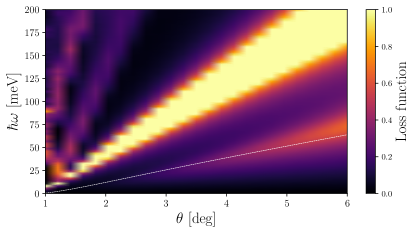
Figure 3: (Color online) The energy loss function ${\cal L}({\bm{q}},\omega)$ of TBG is plotted as a function of the twist angle $\theta$ and frequency $\omega$. Results in this plot have been obtained by keeping fixed the wave number $q$ and filling factor $\nu$, i.e.  $q=q_{\theta}\equiv 2|\bm{K}_{1,2}|/31$ (see main text) and $\nu=+1$. Bright bands correspond to plasmons peaks. The white dashed line indicates the upper edge of the particle-hole continuum, i.e. $\omega=v^{\star}(\theta)q_{\theta}$, $v^{\star}(\theta)$ being the reduced Fermi velocity, above which collective modes are well defined. The low-energy acoustic plasmon mode, which “tracks” the upper edge of the particle-hole continuum, disappears for $\theta\lesssim 2^{\degree}$.

\begin{overpic}[width=216.81pt]{layer_pol_105_V-1.pdf}\put(0.0,55.0){(a)}\end{overpic}

\begin{overpic}[width=216.81pt]{layer_pol_5_V-1.pdf}\put(0.0,55.0){(b)}\end{overpic}

Figure 4: (Color online) Layer polarization ${\cal P}_{\bm{k},\lambda}$ of the Hartree self-consistent eigenstates , superimposed on TBG energy bands calculated with Hartree self-consistency at filling factor $\nu=+1$. Panel (a) $\theta=1.05^{\degree}$. Panel (b) $\theta=5^{\degree}$. At lower angles the Hamiltonian eigenstates are less layer polarized, resulting in more hybridization and the suppression of the bi-layer acoustic plasmon mode. Bands are calculated at the $K^{\prime}$ valley.

Fig. 1 shows the TBG loss function for filling factor $\nu=+1$ and two values of the twist angle $\theta$, i.e. $\theta=1.05^{\degree}$ in panel (a) and $\theta=5^{\degree}$ in panel (b). This filling factor corresponds to a carrier density $n=0.64\times 10^{12}$ cm^-2 for $\theta=1.05^{\degree}$ and $n=1.5\times 10^{13}$ cm^-2 for $\theta=5^{\degree}$. Chemical potential values have been given in the caption of Fig. 1. Close to the magic angle, Fig. 1(a), flat bands centered at the CNP and separated by an energy gap from the higher-energy bands, lead to intrinsically undamped slow plasmons [46]. We clearly see this in Fig. 1(a), where a narrow, almost dispersion-less plasmon is present at energies on the order of $\sim 20~{}{\rm meV}$. In general, we find that, at small twist angles, TBG hosts a standard intra-band COM plasmon with a $\omega_{\rm COM}(q)\propto\sqrt{q}$ dispersion in the long-wavelength limit. No sign of other collective modes is seen at small values of $\theta$, neither gapless [39, 41] nor gapped [42, 43]—further results are reported in Appendix B.

This is not the case for larger values of the twist angle, as seen for example in Fig. 1(b) for $\theta=5^{\degree}$. For this value of the twist angle, an acoustic plasmon is clearly visible. This mode lies just above the upper edge of the particle-hole continuum (Appendix A), which is identified by the line $\hbar\omega_{\theta}(q)=\hbar v^{\star}_{\theta}q$, $v^{\star}_{\theta}$ being the reduced Fermi velocity of the TBG Dirac cones [32]:

$$v^{\star}_{\theta}=v_{\rm D}\frac{1-3\alpha^{2}(\theta)}{1+6\alpha^{2}(\theta)}~{},$$ (44)

$\alpha(\theta)=u_{1}\left[\frac{8\pi}{3a}\hbar v_{\rm D}\sin\left(\frac{\theta}{2}\right)\right]^{-1}$ being a dimensionless parameter that depends on the twist angle (the parameters $v_{\rm D}$ and $u_{1}$ have been introduced in Sect. IV.1). For $\theta=5^{\degree}$, the Fermi velocity (44) is $v_{\theta}^{*}\approx 7.99\times 10^{5}$ m/s, while the acoustic plasmon velocity in Fig. 1(b) is $c_{\rm s}\approx 8.43\times 10^{5}$ m/s. For the sake of comparison, we note that the acoustic plasmon velocity in two (tunnel-decoupled but Coulomb-coupled) graphene layers at a distance $d=0.3$ nm is $c_{\rm s}\approx 1.2\times 10^{6}$ m/s (and at the same density $n=1.5\times 10^{13}$ cm^-2) [41]. A reduced single-particle Fermi velocity in TBG leads to slower acoustic plasmons with respect to other graphene-related systems [41]. A plot illustrating the dependence of $c_{\rm s}$ on $\theta$ is reported in Appendix A.

(Further numerical results are reported in Appendix B—where the plasmon dispersion relation obtained with the inclusion of the layer-pseudospin degree of freedom and LFEs is compared with that obtained by neglecting the latter—and Appendix C— where the dependence on the filling factor $\nu$ is discussed, for various twist angles. In Appendix B, we note that the introduction of LFEs leads to a blue shift in the energy of the plasmon modes around the edge of the moiré BZ, as already found out in other systems [68, 69, 66]. This effect is even more pronounced at small twist angles. In Appendix C, we observe, for a fixed value of $\theta$, a weak dependence on $\nu$.)

Fig. 3 shows the loss function ${\cal L}({\bm{q}},\omega)$ as a function of the twist angle $\theta$ and frequency $\omega$. Results in this figure have been obtained by setting $q=q_{\theta}\equiv\xi|\bm{K}_{1,2}|$, where $|\bm{K}_{1}|=|{\bm{K}}_{2}|$ is the modulus of the $\theta$-depending vector linking $\Gamma$ to $K$ in the moiré BZ—see Eq. (20)—and $\xi=2/31<1$. The brightest feature in this figure corresponds to the usual COM plasmon while the lower-energy feature corresponds to the acoustic plasmon. At twist angles $\theta\lesssim 2^{\degree}$, the acoustic plasmon branch disappears. We conclude that, at small twist angles, low energies, and long wavelengths, TBG behaves effectively as a single 2DES with an ordinary COM plasmon. A weakly-damped out-of-phase acoustic plasmon appears only for twist angles larger than $\theta\approx 2^{\degree}$. As discussed in Sect I, this mode is typical of weakly-coupled double layers, where two spatially-separated 2DESs interact only through the long-range Coulomb interaction [39, 41]. The gapless nature of the extra mode emerging for $\theta\gtrsim 2^{\degree}$ is reasonable since the moiré potential that couples the two layers does not open a gap at the $K$/$K^{\prime}$ points (Dirac cones are protected by symmetry).

Despite the apparent similarity with spatially-separated 2DESs, acoustic plasmons in TBG offer a qualitative difference: in the latter system, they emerge only for sufficiently large values of $\theta$. In the former systems, instead, acoustic plasmons exist for all values of the macroscopic parameters, provided that the single-particle Fermi velocities in the two 2DESs are identical [39, 41].

Regarding damping of the TBG acoustic plasmon, let us recall that the upper edge of the particle-hole continuum in TBG is given by:

$$\hbar\omega_{\theta}(q_{\theta})\equiv\hbar v^{*}_{\theta}q_{\theta}=\xi\frac{8\pi}{3a}\hbar v_{\rm D}\frac{\sin^{2}(\theta/2)-3\tilde{\alpha}^{2}}{\sin^{2}(\theta/2)+6\tilde{\alpha}^{2}}\sin(\theta/2)~{},$$ (45)

where $\tilde{\alpha}=\alpha(\theta)/\sin(\theta/2)$ and $\alpha(\theta)$ has been introduced above in Eq. (44). If the plasmon dispersion lies above this threshold value, it is a well-defined (i.e. long lived) mode (at least within the RPA). Since the wave vector $q$ is fixed at the value $q_{\theta}\equiv\xi|\bm{K}_{1,2}|$, the expression on the right hand side of Eq. (45) depends only on $\theta$ and is plotted in Fig. 3 (white dashed line) for small values of $\theta$ (up to $\theta=6^{\degree}$). We clearly see that, for sufficiently large values of $\theta$ (i.e. $\theta\gtrsim 4^{\degree}$) the acoustic plasmon is a well-defined long-lived collective mode.

In order to better understand the disappearance of the acoustic mode for $\theta\lesssim 2^{\degree}$, we have calculated the layer polarization ${\cal P}_{\bm{k},\lambda}$ of the TBG Hartree self-consistent eigenstates $|\bm{k},\lambda\rangle$. This quantity is defined as [75]:

$${\cal P}_{\bm{k},\lambda}\equiv\langle\bm{k},\lambda|\hat{\Pi}^{(1)}|\bm{k},\lambda\rangle-\langle\bm{k},\lambda|\hat{\Pi}^{(2)}|\bm{k},\lambda\rangle~{},$$ (46)

where $\hat{\Pi}^{(i)}$ is the projector operator onto the $i$-th layer introduced in Sec. IV, Eq. (33). Fig. 4 shows the layer polarization (color bar) at the $K$ valley and for two values of the twist angle, i.e. $\theta=1.05^{\degree}$—panel (a)—and $\theta=5^{\degree}$—panel (b). For the latter value of the twist angle, the polarization is $|{\cal P}_{\bm{k},\lambda}|\approx 1$ for almost every value of the wave vector ${\bm{k}}$ and throughout all the bands. At $\theta=1.05^{\degree}$, instead, we observe a very low layer polarization stemming from a strong inter-layer hybridization. It is this transition from high to low values of the layer polarization that, in our opinion, leads to the disappearance of the acoustic plasmon mode at twist angles $\theta\lesssim 2^{\degree}$.

VI Summary and conclusions

In this Article we have presented a theoretical study of the plasmonic response of twisted bilayer graphene as a function of the twist angle $\theta$. Our theory treats on equal footing four important effects, namely the layer degree of freedom, non-local effects in the density-density response function beyond the dynamical long-wavelength limit, Hartree self-consistency, and crystalline local field effects.

We have found that at small values of the twist angle ($\theta\lesssim 2^{\degree}$) and in the low-energy long-wavelength limit, the 2D electron system in twisted bilayer graphene responds to a perturbation carrying wave vector $q$ and energy $\hbar\omega$ as a single entity, displaying a center-of-mass mode $\omega_{\rm COM}(q)\propto\sqrt{q}$. This is in agreement with all earlier studies [44, 45, 46, 47]. As the twist angle increases, however, inter-layer tunneling decreases and the layer-pseudospin becomes a quasi-good quantum number. For $\theta\gtrsim 2^{\degree}$, the layer-pseudospin degree of freedom needs to be taken into account and the plasmonic spectrum of the system displays a qualitatively different behavior. In this case, indeed, a weakly-damped acoustic plasmon mode appears, akin to the acoustic plasmon of other parallel 2D electron systems of historical importance [38, 39].

In the future it will be interesting to feed our results to an Eliashberg theory [76] of plasmon-mediated superconductivity in twisted bilayer graphene and to study the spatial distribution of chirality associated to this mode [77, 78].

Appendix A Acoustic plasmons and the TBG particle-hole continuum

In this Appendix we show that the acoustic plasmon appearing in Fig. 1(b) of the main text lies above the TBG particle-hole continuum (and it is therefore undamped). As discussed in the main text, the upper edge of such continuum is identified by $\hbar\omega_{\theta}=\hbar v^{*}_{\theta}q$. In Figs. A1(a) and (b) we report the plasmon spectrum of TBG for $\theta=5^{\circ}$ and $\theta=6^{\circ}$, respectively. In each panel, the white dashed line represents the $\hbar\omega_{\theta}=\hbar v^{*}_{\theta}q$ line. We clearly see that, for both twist angles, the acoustic plasmon mode lies above the particle-hole continuum, although falls very close to it.

\begin{overpic}[width=216.81pt]{zoom_loss_function_5_filling0.25_GKM.pdf}\put(0.0,54.0){(a)}\end{overpic}

\begin{overpic}[width=216.81pt]{zoom_loss_function_6_filling0.25_GKM.pdf}\put(0.0,54.0){(b)}\end{overpic}

Figure A1: (Color online) The TBG energy loss function ${\cal L}({\bm{q}},\omega)$ is plotted as a function of ${\bm{q}}$ (along the $\Gamma-K$ high symmetry path) and $\omega$ for two values of the twist angle $\theta$: $\theta=5\degree$ in panel (a) and $\theta=6\degree$ in panel (b). Results in this plot refer to filling factor $\nu=+1$ and temperature $T=5~{}{\rm K}$. The upper edge of the particle-hole continuum (which of course depends on $\theta$), i.e. $\omega=v^{\star}_{\theta}q$, $v^{\star}_{\theta}$ being the reduced Fermi velocity (see Eq. (44) in the main text), is represented by a thin white dashed line.

A plot summarizing the dependence of $c_{\rm s}$ on $\theta$ is reported in Fig. A2.

\begin{overpic}[width=216.81pt]{c_s_vs_theta.pdf}\put(58.0,11.0){{\color[rgb]{1,1,1} Particle-hole continuum}} \end{overpic}

Figure A2: (Color online) The sound velocity $c_{\rm s}$ (red stars) of the acoustic plasmon is plotted as a function of the twist angle $\theta$. Results in this plot have been obtained by setting $\nu=+1$ and $T=5$ K. The shaded region identifies the particle-hole continuum, whose upper edge coincides with $v^{\star}_{\theta}$ (see Eq. (44) in the main text). The horizontal solid line represents the acoustic plasmon velocity in two spatially-separated graphene layers [41] at a distance $d=0.3$ nm and total electron density of $n=1.5\times 10^{13}$ cm^-2.

Appendix B Impact of LFEs on the plasmonic spectrum

In this Appendix we discuss the role of LFEs on the plasmonic spectrum. Results presented in Figs. A3 and A4 have been obtained by setting $\varepsilon_{1}=\varepsilon_{3}=4.9$, $\varepsilon_{2}=1$, and $T=5~{}{\rm K}$. In order to isolate the impact of LFEs, we have deliberately neglected Hartree corrections in producing the data reported in Figs. A3 and A4.

Fig. A3 compares the energy loss function (for $\theta=1.35^{\degree}$ and various values of $\nu$) in the local (i.e.  $\bm{G}=\bm{G}^{\prime}=\bm{0}$) approximation (panels in the right column) with that calculated by including LFEs (panels in the left columns). The impact of LFEs is most significant around the edges of the moiré BZ. This is especially true at low doping.

A similar comparison is reported in Fig. A4 where the filling factor is fixed at $\nu=+1$ while the twist angle is varied. Increasing the angle leads to a reduction of the importance of LFEs corrections. As emphasized in the main text, for $\theta=6^{\degree}$ we can clearly see the acoustic plasmon mode.

\begin{overpic}[width=216.81pt]{hr_loss_function_1.35_filling0.0_GKM.pdf}\put(0.0,43.0){(a)}\end{overpic}	\begin{overpic}[width=216.81pt]{hr_local_loss_function_1.35_filling0.0_GKM.pdf}\put(0.0,43.0){(b)}\end{overpic}
\begin{overpic}[width=216.81pt]{hr_loss_function_1.35_filling0.25_GKM.pdf}\put(0.0,43.0){(c)}\end{overpic}	\begin{overpic}[width=216.81pt]{hr_local_loss_function_1.35_filling0.25_GKM.pdf}\put(0.0,43.0){(d)}\end{overpic}
\begin{overpic}[width=216.81pt]{hr_loss_function_1.35_filling0.5_GKM.pdf}\put(0.0,43.0){(e)}\end{overpic}	\begin{overpic}[width=216.81pt]{hr_local_loss_function_1.35_filling0.5_GKM.pdf}\put(0.0,43.0){(f)}\end{overpic}

Figure A3: (Color online) The TBG energy loss function ${\cal L}({\bm{q}},\omega)$ is plotted as a function of ${\bm{q}}$ and $\omega$ for $\theta=1.35^{\degree}$ and various filling factors $\nu$. Results shown in the panels on the left (right) column have been obtained by including (neglecting) LFEs. Panels (a)-(b): $\nu=0$. Panels (c)-(d): $\nu=+1$. Panels (e)-(f): $\nu=+2$. On the horizontal axis we report ${\bm{q}}$ along the high-symmetry path $\Gamma$-$K$-$M$ of the moiré BZ—see Fig. 2(b) in the main text.

\begin{overpic}[width=216.81pt]{loss_function_105_filling0.25_GKM.pdf}\put(0.0,43.0){(a)}\end{overpic}	\begin{overpic}[width=216.81pt]{local_loss_function_105_filling0.25_GKM.pdf}\put(0.0,43.0){(b)}\end{overpic}
\begin{overpic}[width=216.81pt]{hr_loss_function_200_filling0.25_GKM.pdf}\put(0.0,43.0){(c)}\end{overpic}	\begin{overpic}[width=216.81pt]{hr_local_loss_function_200_filling0.25_GKM.pdf}\put(0.0,43.0){(d)}\end{overpic}
\begin{overpic}[width=216.81pt]{hr_loss_function_6_filling0.25_GKM.pdf}\put(0.0,43.0){(e)}\end{overpic}	\begin{overpic}[width=216.81pt]{hr_local_loss_function_6_filling0.25_GKM.pdf}\put(0.0,43.0){(f)}\end{overpic}

Figure A4: (Color online) The TBG energy loss function ${\cal L}({\bm{q}},\omega)$ is plotted as a function of ${\bm{q}}$ and $\omega$ for $\nu=+1$ and various values of the twist angle $\theta$. Results in the left column (i.e. panels (a), (c), and (e)) have been obtained by including LFEs. Results in the right column (i.e. panels (b), (d), and (f)) have been obtained by neglecting LFEs. Panels (a)-(b): $\theta=1.05^{\degree}$. Panels (c)-(d): $\theta=2^{\degree}$. Panels (e)-(f): $\theta=6^{\degree}$. On the horizontal axis we report ${\bm{q}}$ along the high-symmetry path $\Gamma$-$K$-$M$ of the moiré BZ—see Fig. 2(b) in the main text.

Appendix C Robustness of the plamonic spectrum with respect to changes in the filling factor

In this Appendix we study the robustness of the acoustic plasmon with respect to changes in the filling factor (exploring, in particular, higher values of $\nu$, as compared to the main text).

We evaluated the energy loss function ${\cal L}({\bm{q}},\omega)$ with LFEs and Hartree corrections (while taking into account the layer-pseudospin degree of freedom) for $\theta=1.05^{\degree}$ and $\theta=5^{\degree}$, at filling factor $\nu=+2$. Results are shown in Figure A5. Similarly to Fig. 1 (which refers to $\nu=+1$), we clearly see an intrinsic acoustic plasmon mode for $\theta=5^{\degree}$. Note that the peak in the energy loss function associated to the acoustic plasmon is weaker for $\nu=+2$ than $\nu=+1$.

Figure A6 shows the energy loss function for different values of $\nu$ and fixed values of the wave vector ${\bm{q}}$ taken along the $\Gamma$-$K$ direction in the moiré BZ. Results in Fig. A6 have been obtained by neglecting the Hartree contribution. In Figure A7 we show similar results—for two values of $\theta$, i.e. $\theta=1.05^{\degree}$ and $\theta=5^{\degree}$—but this time with the inclusion of the Hartree contribution. Note the very high level of particle-hole symmetry in the plasmonic spectrum and a significant suppression of the acoustic plasmon for $|\nu|>2$.

\begin{overpic}[width=216.81pt]{hrH_loss_function_1.05_filling0.5_GKM.pdf}\put(0.0,43.0){(a)}\end{overpic} \begin{overpic}[width=216.81pt]{hr_loss_function_5_filling0.5_GKM.pdf}\put(0.0,43.0){(b)}\end{overpic}

Figure A5: (Color online) The TBG energy loss function ${\cal L}({\bm{q}},\omega)$ is plotted as a function of ${\bm{q}}$ and $\omega$ for $\nu=+2$. Results in this figure have been obtained by taking into account both LFEs and Hartree corrections. Panel (a) $\theta=1.05^{\degree}$. Panel (b) $\theta=5^{\degree}$. On the horizontal axis we report ${\bm{q}}$ along the high-symmetry path $\Gamma$-$K$-$M$ of the moiré BZ—see Fig. 2(b) in the main text.

\begin{overpic}[width=216.81pt]{loss_function_105_vs_filling.pdf}\put(0.0,53.0){(a)}\end{overpic}	\begin{overpic}[width=216.81pt]{loss_function_135_vs_filling.pdf}\put(0.0,53.0){(b)}\end{overpic}
\begin{overpic}[width=216.81pt]{loss_function_200_vs_filling.pdf}\put(0.0,53.0){(c)}\end{overpic}	\begin{overpic}[width=216.81pt]{loss_function_500_vs_filling.pdf}\put(0.0,53.0){(d)}\end{overpic}

Figure A6: (Color online) The TBG energy loss function ${\cal L}({\bm{q}},\omega)$ is plotted as a function of $\omega$ and filling factor $\nu$. Each panel corresponds to a value of $\theta$ and $q$ (the latter taken along the $\Gamma$-$K$ direction of the moiré BZ). Results in this figure have been obtained by neglecting Hartree corrections. Panel (a) $\theta=1.05^{\degree}$. Panel (b) $\theta=1.35^{\degree}$. Panel (c) $\theta=2^{\degree}$. Panel (d) $\theta=5^{\degree}$.

\begin{overpic}[width=216.81pt]{loss_function_105_vs_filling_hartree.pdf}\put(0.0,53.0){(a)}\end{overpic}

\begin{overpic}[width=216.81pt]{loss_function_500_vs_filling_hartree.pdf}\put(0.0,53.0){(b)}\end{overpic}

Figure A7: (Color online) The TBG energy loss function ${\cal L}({\bm{q}},\omega)$ is plotted as a function of $\omega$ and filling factor $\nu$. Each panel corresponds to a value of $\theta$ and $q$ (the latter taken along the $\Gamma$-$K$ direction of the moiré BZ). Results in this figure have been obtained by including Hartree corrections. Panel (a) $\theta=1.05^{\degree}$. Panel (b) $\theta=5^{\degree}$.