Analytic Model for Molecules Under Collective Vibrational Strong Coupling in Optical Cavities

Abstract

Analytical results are presented for a model system consisting of an ensemble of $N$ molecules under vibrational strong coupling (VSC). The single bare molecular model is composed of one effective electron, which couples harmonically to multiple nuclei. A priori no harmonic approximation is imposed for the inter-nuclear interactions. Within the cavity Born-Oppenheimer partitioning, i.e., when assuming classical nuclei and displacement field coordinates, the dressed $N$-electron problem can be solved analytically in the dilute limit. In more detail, we present a self-consistent solution of the corresponding cavity-Hartree equations, which illustrates the relevance of the non-perturbative treatment of electronic screening effects under VSC. We exemplify our derivations for an ensemble of harmonic model CO₂ molecules, which shows that common simplifications can introduce non-physical effects (e.g., a spurious coupling of the transverse field to the center-of-mass motion for neutral atoms). In addition, our self-consistent solution reveals a simple analytic expression for the cavity-induced red shift and the associated refractive index, which can be interpreted as a polarizability-dependent detuning of the cavity. Finally, we highlight that anharmonic intra-molecular interactions might become essential for the formation of local strong coupling effects within a molecular ensemble under collective VSC.

I Introduction

Polaritonic chemistry is an emerging field of research at the interface between quantum optics, quantum chemistry and materials science [1, 2, 3]. By placing matter in a photonic environment, e.g., a Fabry-Pérot cavity, it has been shown experimentally that chemical and material properties can be modified. Among others this includes, energy transport [4], photo-chemical reactions [5] and also ground-state chemical reactions [6]. All of these results can happen in the ”dark”, that is, without external illumination. Which degrees of freedom are affected can be controlled by the resonances of the photonic structure, e.g., for Fabry-Pérot cavities that is by changing the length of the cavity $L$, the effective refractive index of the medium $n_{r}$ inside the cavity or by changing the mode order $m$, such that the wavelength of the cavity resonances become

$$\Lambda=\frac{2n_{r}L}{m}.$$ (1)

Specifically the case of ground-state chemical reactions, where the wavelength $\Lambda$ of the cavity is in the infrared (ro-vibrational) regime, has attracted considerable interest [3, 7, 8, 9]. While significant experimental progress has been reported, the theoretical description is far from complete. Since most of these experiments are in the collective regime, that is, a large amount of molecules inside the cavity couple to the resonance of the cavity, the theoretical description needs to take a very large amount of molecules into account at the same time. This is in stark contrast to, for instance, the case of a dilute gas in free space, where one can consider a single molecule and perform a statistic treatment of the total ensemble by assuming that the molecules are largely uncorrelated. In the case of strong coupling, a priori a treatment of the full ensemble including cavity-induced inter-molecular correlations effects seems necessary. For computational reasons, however, usually only either a single or a few molecules are considered accurately (with unrealistically scaled-up coupling constant) or alternatively large ensemble sizes can be reached with strong simplifications on the coupling and matter description (e.g., Tavis-Cumming-like coupling scheme [7, 8, 9]). Both approaches have intrinsic limitations and are not yet able to full capture all the details of the experimental observations. Among others it remains unclear how in the collective regime individual molecules of the total ensemble are changed. Recently, a feedback and local-polarization mechanism akin to a spin-glass has been discovered, [10] by taking the electronic as well as the nuclear structure of the full ensemble into account self-consistently [10, 11, 12]. Among others, this effect could explain the changes in dispersion forces, which critically depend on also the electronic polarization of the molecule, as recently observed in experiment [13].

In this work, to get a better understanding of how this feedback and polarization mechanism manifests itself in vibrational strong coupling (VSC), we develop a simple ab initio model of an ensemble of molecules that allows for simple analytical results. To do so, we assume harmonic (effective) electrons such that the cavity Born-Oppenheimer approximation (cBOA) allows an analytic self-consistent solution of the electrons of the full ensemble. By doing so we highlight differences to common approximations. Among others, we find that only upon a self-consistent treatment of the electrons with the nuclei, we obtain the experimentally observed red-shift of the coupled light-matter resonance. We analyze properties of the self-consistently coupled ensemble for a simple harmonic model of CO₂ molecules, such that the classical and the quantum equations of motion are the same. Finally we argue that anharmonicities are essential to unambiguously identify local strong coupling effects in a molecular ensemble under collective VSC. Eventually, we discuss the implications of real electronic structures on VSC: For real molecules, a non-trivial feedback effect is expected between the translational and vibrational modes. This mechanism could become particularly important at ambient temperature, where bare vibrational modes could only be scarcely populated (modified) otherwise.

II Self-consistent harmonic model for collective VSC

In the following we investigate collective VSC in a minimal ab initio molecular setting, which allows an (semi)-analytic treatment. For this purpose we look at an ensemble of $N$ identical, non-interacting effective one-dimensional molecules, each one consisting of a single effective electron with negative charge $-Z_{e}|e|$ and $N_{n}$ nuclei of mass $M_{n}$ and with positive charge $Z_{n}|e|$. The corresponding bare matter Hamiltonian is given by

$$\hat{H}_{\rm m}\!\!=\!\sum_{i=1}^{N}\!\!\Bigg{[}\!\sum_{n=1}^{N_{n}}\!\bigg{(}\frac{\hat{P}_{in}^{2}}{2M_{n}}\!+\!\frac{k_{e}}{2}(\hat{R}_{in}\!-\!\hat{r}_{i})^{2}\bigg{)}\!+\!\frac{\hat{p}_{i}^{2}}{2}\!+\!V(\bm{\hat{R}}_{i})\!\Bigg{]}.$$ (2)

The molecular ensemble will be collectively coupled to a single effective cavity mode $\beta$, e.g., of a Fabry-Pérot cavity. In the length gauge, the Pauli-Fierz Hamiltonian for this system is then given by

$$\hat{H}=\hat{H}_{\rm m}+\frac{1}{2}\bigg{[}\hat{p}_{\beta}^{2}+\omega_{\beta}^{2}\Big{(}\hat{q}_{\beta}-\frac{\hat{X}+\hat{x}}{\omega_{\beta}}\Big{)}^{2}\bigg{]}.$$ (3)

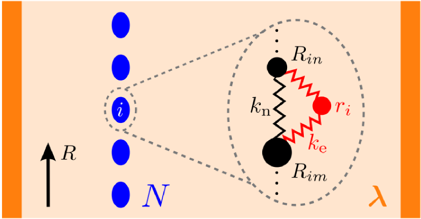
Figure 1: Sketch of the model setup shows cavity (single mode $\beta$ with energy $\omega_{\beta}$ parallel polarized to the matter coordinate axis) with $N$ identical molecules far apart from each other, made up of $N_{\mathrm{n}}$ (different) nuclei and one effective electron of charge $Z_{\mathrm{e}}$ bound together by potentials, which later will be associated with force constants $k_{\mathrm{n}}$ between the nuclei and $k_{\mathrm{e}}$ between nuclei and effective electron, respectively. The nuclei and electron interact with the cavity via the coupling constant $\lambda$.

Notice, the reason why we consider this a minimal molecular model will become clear later (see Sec.  II.1), where we show that the restriction to a single nuclei would show a qualitatively different behavior. We define coupled polarization operators as $\hat{X}:=\lambda\sum_{i=1}^{N}\sum_{n=1}^{N_{n}}Z_{n}\hat{R}_{in}$ and $\hat{x}:=-\lambda\sum_{i=1}^{N}Z_{e}\hat{r}_{i}$, where the nuclear and electronic total transition dipole moments, respectively, are coupled via $\lambda$ to the effective photon mode of frequency $\omega_{\beta}$ (with corresponding photonic displacement $\hat{q}_{\beta}$ and canonical momentum/magnetic $\hat{p}_{\beta}$ operators). We note that for the ground-state chemical reactions the effective single-mode approximation is expected to capture all the essential physics [14, 15]. The main effect of a proper continuum of modes amounts to an extra dissipation channel as this leads to the radiative decay of the coupled system [16, 9]. Nuclear position/displacement and momentum operators are indicated by capital letters, whereas for the $i$-th electron $\hat{p}_{i}$ and $\hat{r}_{i}$ are used, respectively. The local nucleus-nucleus interaction $V(\bm{\hat{R}}_{i})$ with $\bm{\hat{R}}_{i}=(\hat{R}_{i1},...,\hat{R}_{iN_{n}})$ will be later parameterized by the force constant $k_{n}$ (see the specific example given in Eq. (31)), whereas the coupling of the single electron to the nuclei is parameterized by the force constant $k_{e}$. The vectorial photon-matter coupling $\bm{\lambda}_{\beta}=\bm{\varepsilon}_{\beta}\lambda$ depends on the mode polarization vector $\bm{\varepsilon}_{\beta}$ and the coupling constant [9]

$$\lambda=\sqrt{\frac{e^{2}}{\mathcal{V}\varepsilon_{0}}}$$ (4)

where $\mathcal{V}$ corresponds to the effective mode volume. This effective mode volume can be connected to properties of the Fabry-Pérot cavity and scales roughly as $L^{3}\mathcal{F}$, where $\mathcal{F}$ is the finesse of the cavity [15]. Here we have assumed for simplicity that all effective one-dimensional molecules are perfectly aligned with respect to the polarization vector $\bm{\varepsilon}_{\beta}$. However, qualitatively similar results are expected for randomly oriented molecules as has previously been shown numerically in Ref. [10].

If we would restrict to purely harmonic nucleus-nucleus interactions (as we do later in Sec. II.2) we could in principle consider the full quantum dynamics by merely solving the corresponding classical equations of motion due to the harmonic nature of the model. Yet, as we discuss afterwards in Sec. IV, anharmonicities can become essential and hence we keep the nucleus-nucleus interaction general at this point. Moreover, we want to connect to the cavity Born-Opphenmeiner approximation (cBOA) [17, 9], where we assume that the electrons adapt instantaneously on the time-scale of the nuclei and displacement coordinate. Thus we partition our polaritonic problem into two coupled sub-problems, one for the electrons and one for the nuclear and displacement degrees of freedom. For the moment we neglect all non-adiabatic couplings and assume only the electronic ground-state energy surface plays a role similar to Ref. [10]. The Hamiltonian operator of the coupled nuclear-photon degrees of freedom of the $l$-the electronic potential energy surface is given by

$$\hat{H} {}^{\mathrm{npt},l}:=\sum_{i=1}^{N}\Bigg{[}\sum_{n=1}^{N_{n}}\bigg{(}\frac{\hat{P}_{in}^{2}}{2M_{n}}+\frac{k_{e}}{2}\hat{R}_{in}^{2}\bigg{)}+V(\bm{\hat{R}}_{i})\Bigg{]}$$ (5)

$$+\frac{\hat{p}_{\beta}^{2}}{2}+\frac{\omega_{\beta}^{2}}{2}\Big{(}\hat{q}_{\beta}-\frac{\hat{X}}{\omega_{\beta}}\Big{)}^{2}+\underbrace{\bra{\Psi_{l}}\hat{H}^{\mathrm{e}}(\bm{R},q_{\beta})\ket{\Psi_{l}}}_{=E^{\rm e}_{l}(\bm{R},q_{\beta})}.$$

The corresponding $N$-electron Hamiltonian operator is given by

$$\hat{H}^{\rm e}(\bm{R},q_{\beta}):=\sum_{i=1}^{N} \Bigg{[}\frac{\hat{p}_{i}^{2}}{2}-\sum_{n=1}^{N_{n}}k_{e}R_{in}\hat{r}_{i}+N_{n}k_{e}\frac{\hat{r}_{i}^{2}}{2}\Bigg{]}$$

$$+\bigg{(}\frac{1}{2}\hat{x}^{2}+\hat{x}X-\omega_{\beta}\hat{x}q_{\beta}\bigg{)},$$ (6)

where the electrons only interact due to the presence of the strongly coupled cavity modes. The electronic Hamiltonian depends only parametrically on all the nuclei positions and displacement field coordinates, written compactly as $(\bm{R},q_{\beta})$.

Assuming the dilute gas limit, the many-electron wave function $\Psi$ reduces to a Hartree product (which can be formally shown starting from a Slater determinant) $\Psi=\psi_{1}\otimes\psi_{2}\otimes\dots\otimes\psi_{i}\otimes\dots\otimes\psi_{N}$ of $N$ single-molecule electronic wave functions $\psi_{i}$, which are determined by the following coupled $N$ Hartree equations [10, 11]

$$\bigg{(}\frac{\hat{p}_{i}^{2}}{2}-\sum_{n=1}^{N_{n}}k_{e}R_{in}\hat{r}_{i}+N_{n}k_{e}\frac{\hat{r}_{i}^{2}}{2}$$ (7)

$$+\Big{(}X-q_{\beta}\omega_{\beta}\!+\!\!\sum_{j\neq i}^{N}\matrixelement{\psi_{j}}{\hat{x}_{j}}{\psi_{j}}\Big{)}\hat{x}_{i}+\frac{\hat{x}_{i}^{2}}{2}\bigg{)}\psi_{i}=\varepsilon_{i}\psi_{i}\mbox{\quad.\quad}$$

The total electronic energy is then the sum of the single molecule energies $E^{\rm e}=\sum_{i}^{N}\epsilon_{i}$.

Thanks to our harmonic matter description, the $N$-electron problem given in Eq. (7) can be solved analytically. By defining $\mu_{i}:=\lambda\sum_{j\neq i}^{N}\matrixelement{\psi_{j}}{\hat{r}_{j}}{\psi_{j}}$, the $i$-th electron problem corresponds to a shifted harmonic oscillator parametrized by $(\bm{R}_{i},q_{\beta})$ as

$$\bigg{[} \frac{\hat{p}_{i}^{2}}{2}+\nu_{1,i}\hat{r}_{i}+\frac{\nu_{2}^{2}}{2}\hat{r}_{i}^{2}\bigg{]}\psi_{i}(r_{i})=\epsilon_{i}\psi_{i}(r_{i}),$$ (8)

$$\nu_{1,i} :=-k_{e}\sum_{n=1}^{N_{n}}R_{in}+Z_{e}(-\lambda X+\lambda\omega_{\beta}q_{\beta}+\lambda Z_{e}\mu_{i})$$ (9)

$$\nu_{2} :=\sqrt{\lambda^{2}Z_{e}^{2}+N_{n}k_{e}}$$ (10)

The shifted harmonic oscillator energies are then

$$\epsilon^{l}_{i} =\expectationvalue{\left(\hat{b}_{i}^{\dagger}\hat{b}_{i}+\frac{1}{2}-\eta_{i}^{2}(\bm{R},q_{\beta})\right)\nu_{2}}_{l}$$

$$=\left(l+\frac{1}{2}\right)\nu_{2}-\eta_{i}^{\prime 2}(\bm{R},q_{\beta})$$ (11)

$$\eta_{i}^{\prime}(\bm{R},q_{\beta})=\frac{\nu_{1,i}}{\sqrt{2}\nu_{2}}=\eta_{i}\sqrt{\nu_{2}}$$ (12)

$$\hat{b}_{i}^{\dagger}=\hat{a}_{i}^{\dagger}+\eta_{i}\,,\quad\hat{b}_{i}=\hat{a}_{i}+\eta_{i}$$ (13)

where $\hat{a}_{i}^{\dagger}=\sqrt{\nu_{2}/2}(\hat{r}_{i}-i\hat{p}_{i}/\nu_{2})$ and $\hat{a}_{i}=\sqrt{\nu_{2}/2}(\hat{r}_{i}+i\hat{p}_{i}/\nu_{2})$ correspond to the ladder operators of the original quantum harmonic oscillator with $\hat{r}_{i}=\sqrt{1/2\nu_{2}}(\hat{a}_{i}^{\dagger}+\hat{a}_{i})$. The solutions of the shifted quantum harmonic oscilltor are connected to the original harmonic oscillator via the unitary displacement operator $\hat{D}_{i}=e^{-\eta_{i}\left(\hat{a}_{i}^{\dagger}-\hat{a}_{i}\right)}$.

Since the instantaneous dipoles of the electrons couple to the cavity field we determine the expectation value of the local and the total electric dipole for later reference. When calculating the electronic position expectation value of the $i$-th electron in the ground state, we find a recursive dependency on the position of all other electrons due to the dipole-dipole interaction term, i.e.,

$$\langle\hat{r}_{i}\rangle_{l}=\langle\hat{r}_{i}\rangle_{0}=-\sqrt{\frac{1}{2\nu_{2}}}(\eta_{i}+\eta_{i}^{*})=-\frac{\nu_{1,i}}{\nu_{2}^{2}}$$ (14)

$$=\frac{1}{N_{n}k_{e}+Z_{e}^{2}\lambda^{2}}\bigg{(}k_{e}\sum_{n=1}^{N_{n}}R_{in}+Z_{e}\bigg{(}\lambda X-\lambda\omega_{\beta}q_{\beta}$$

$$-\lambda^{2}Z_{e}\Big{(}\sum_{j}^{N}\langle\hat{r}_{j}\rangle_{0}-\langle\hat{r}_{i}\rangle_{0}\Big{)}\bigg{)}\bigg{)}$$ (15)

$$=\frac{1}{N_{n}}\bigg{(}\sum_{n=1}^{N_{n}}R_{in}+\frac{\lambda Z_{e}}{k_{e}}\Big{(}X+\langle x\rangle_{0}-\omega_{\beta}q_{\beta}\Big{)}\bigg{)}$$ (16)

$$=\frac{1}{N_{n}}\bigg{(}\sum_{n=1}^{N_{n}}R_{in}-\frac{E_{\perp}Z_{e}}{k_{e}}\bigg{)}$$ (17)

where in the last step the definition of the transverse electric field

$$E_{\perp}=\lambda(\omega_{\beta}q_{\beta}-X-\langle x\rangle)$$ (18)

in the length gauge in terms of the displacement and polarization fields was introduced [18, 9]. Thus we can re-write the transverse electric field in terms of local molecular quantities as

$$E_{\perp}=\frac{k_{e}}{Z_{e}}\bigg{(}\sum_{n=1}^{N_{n}}R_{in}-N_{n}\langle r_{i}\rangle\bigg{)}$$ (19)

We note that if we would only couple to the displacement field without including the self-consistent polarization of the system, i.e., we do not have the dipole self-energy in Eq. (3) but only keep $-\omega_{\beta}\hat{q}_{\beta}(\hat{X}+\hat{x})$, then we would find due to $\nu_{1,i}\rightarrow-k_{e}\sum_{n}R_{in}+Z_{e}\lambda\omega_{\beta}q_{\beta}$ and $\nu_{2}\rightarrow\sqrt{N_{n}k_{e}}$

$$\langle\hat{r}_{i}^{\rm TC}\rangle\rightarrow\frac{1}{N_{n}}\bigg{(}\sum_{n=1}^{N_{n}}R_{in}-\frac{\omega_{\beta}q_{\beta}\lambda Z_{e}}{k_{e}}\bigg{)}.$$ (20)

We would obtain the same result if we replaced the displacement field by an external electric field instead. In more detail, via $-\omega_{\beta}\hat{q}_{\beta}(\hat{X}+\hat{x})\rightarrow-E_{\rm ext}(\hat{X}+\hat{x})|e|/\lambda$ we could just replace $\omega_{\beta}q_{\beta}\lambda\rightarrow E_{\rm ext}|e|$ in Eq. (20). We note that this is only possible because we have a harmonic potential, which becomes arbitrarily strong as we move away from the minimum of the binding potential. For more realistic (Coulombic) potentials, which approach a finite value for $|r_{i}|\rightarrow\infty$, such dipolar couplings would become problematic since no ground state would exist in an ab initio description [19, 20]. If we further assumed, as often done in polaritonic chemistry for VSC [7, 8, 9], that the electronic structure would not be affected, one could simplify further, using the bare matter electronic structure solutions. Accordingly, we would obtain

$$\langle\hat{r}_{i}^{\rm bare}\rangle\rightarrow\frac{1}{N_{n}}\sum_{n=1}^{N_{n}}R_{in}.$$ (21)

due to $\nu_{1,i}\rightarrow-k_{e}\sum_{n}R_{in}$ and $\nu_{2}\rightarrow\sqrt{N_{n}k_{e}}$.

Having determined $\langle\hat{r}_{i}\rangle$ self-consistently in Eq. (16), we can perform the $\lambda$-weighted summation over all $N$ molecules to obtain the following exact relation

$$\langle x\rangle\underbrace{\bigg{(}1+\frac{\lambda^{2}Z_{e}N}{N_{n}k_{e}}\bigg{)}}_{=\gamma^{-2}} =-\frac{\lambda Z_{e}}{N_{n}}\sum_{i=1}^{N}\sum_{n=1}^{N_{n}}R_{in}-\frac{\lambda^{2}Z_{e}^{2}N}{N_{n}k_{e}}X$$

$$+\frac{\lambda^{2}Z_{e}^{2}N}{N_{n}k_{e}}\omega_{\beta}q_{\beta}.$$ (22)

This allows us to rewrite the transverse electric field given in Eq. (18) solely in terms of nuclear and displacement field coordinates such that we will find self-consistent equations of motion for the combined nuclei-displacement subsystem. We will do so for a specific harmonic model of a molecule in the next section. For the case of zero polarization of matter, i.e., we discard the dipole self-energy term, we trivially have $E_{\perp}=\lambda\omega_{\beta}q_{\beta}$. We note that this is an intrinsic assumption of various approximations such as the Tavis-Cummings model [18, 9].

II.1 Microscopic description of VSC

Based on these considerations, we first reach for a local understanding of the coupled dynamics. In general, when we have anharmonic systems (due to anharmonicities in the electron-nucleus or nucleus-nucleus interaction), the classical and the quantum equations of motion will differ and we have to consider, e.g., hierarchical equations of motion [21, 22]. However, since we will later employ also an harmonic nuclear system, we focus here on the classical equations of motion. For this purpose, we use the Hellmann-Feynman theorem applied to the original Hamiltonian given in Eq. (3). The force acting on the $n$-th nucleus in molecule $i$ on the $l$-th PES becomes,

$$M_{n}\ddot{R}_{in} = -\frac{d}{dR_{in}}\langle\hat{H}\rangle_{l}=-\langle\Big{(}\frac{d}{dR_{in}}\hat{H}\Big{)}\rangle_{l}$$ (24)

$$= -\frac{d}{dR_{in}}V(\bm{R}_{i})-k_{e}(R_{in}-\langle\hat{r}_{i}\rangle_{l})$$

$$+\omega_{\beta}\Bigg{(}q_{\beta}-\bigg{(}\frac{X+\langle\hat{x}\rangle_{l}}{\omega_{\beta}}\bigg{)}\Bigg{)}\lambda Z_{n}.$$

In a next step, we relate the forces to the transverse electric field, which yields the following local equation of motion for the $n$-th nucleus of molecule $i$:

$$M_{n}\ddot{R}_{in} \overset{\rm Eq.\eqref{eq:rietrans}}{=} -\frac{d}{dR_{in}}V(\bm{R}_{i})-k_{e}\bigg{(}R_{in}-\sum_{m=1}^{N_{n}}\frac{R_{im}}{N_{n}}\bigg{)}$$ (25)

$$+\bigg{(}Z_{n}-\frac{Z_{e}}{N_{n}}\bigg{)}E_{\perp}.$$

Notice that the first line contains purely intra-molecular forces (that are present even without a cavity), whereas the second line corresponds to forces that are solely collective and induced by the cavity. As a sanity check, we immediately find that for neutral atoms, where we have only a single nucleus and thus $N_{n}=1$ and $Z_{e}=Z_{N}$, the nuclear motion is not influenced by the cavity. Therefore we need to have a dedicated molecular model that is not just an adapated atomic model.

Before we move on, we compare two different approximations employed in polaritonic chemistry. If we took the full equation based on the Pauli-Fierz Hamiltonian of Eq. (3) and substitute the bare electronic structure from Eq. (21), we would spuriously find,

$$M_{n}\ddot{R}_{in}^{\rm bare} =-\frac{d}{dR_{in}}V(\bm{R}_{i})-k_{e}\bigg{(}R_{in}-\sum_{m=1}^{N_{n}}\frac{R_{im}}{N_{\mathrm{n}}}\bigg{)}$$ (26)

$$+Z_{n}\lambda\Bigg{(}\omega_{\beta}q_{\beta}-\bigg{(}\lambda\sum_{i=1}^{N}\sum_{m=1}^{N_{n}}\bigg{(}Z_{m}-\frac{Z_{e}}{N_{n}}\bigg{)}R_{im}\bigg{)}\Bigg{)},$$

where we have used $\langle\hat{x}\rangle=-\lambda\sum_{i=1}^{N}Z_{e}\langle\hat{r}_{i}^{\rm bare}\rangle=-\lambda Z_{e}\sum_{i}\sum_{n}R_{in}/N_{n}$. Thus, when neglecting the exact polarization of the electronic structure, non-physical effects emerge, which for example suggest the spurious coupling of a neutral atoms to the cavity within the dipole approximation.

Alternatively, an often employed approximation is to consistently discard the dipole self-interaction term from the very beginning and thus assumes non-polarizable matter. In this case we would discard in Eq. (3) all the dipole self-energy terms and thus would obtain

$$M_{n}\ddot{R}_{in}^{\mathrm{TC}} =-\frac{d}{dR_{in}}V(\bm{R}_{i})-k_{e}(R_{in}-\langle\hat{r}_{i}\rangle)$$ (27)

$$+Z_{n}\lambda\omega_{\beta}q_{\beta}.$$

Using Eq. (20) we find

$$M_{n}\ddot{R}_{in}^{\mathrm{TC}} =-\frac{d}{dR_{in}}V(\bm{R}_{i})-k_{e}\bigg{(}R_{in}-\sum_{n=1}^{N_{n}}\frac{R_{in}}{N_{n}}\bigg{)}$$

$$+\bigg{(}Z_{n}-\frac{Z_{e}}{N_{n}}\bigg{)}\lambda\omega_{\beta}q_{\beta},$$ (28)

which at least is consistent with the exact dynamics of Eq. (25) in the trivial case of neutral atoms. Similarly, when trying to simplify the displaced electronic structure problem further, by using the bare matter results, one would again find a non-physical coupling for the neutral atoms.

These considerations show that common approximation strategies can introduce non-physical behavior in the dynamics of a strongly-coupled ensemble. Of specific importance is to employ a self-consistent treatment of the electronic structure in the cavity in such cases.

II.2 CO₂ under collective VSC

It is now interesting to understand the feedback on the nuclear and photonic displacement degrees of freedom due to the self-consistent electronic structure for a specific chemical setup. For this purpose we consider a symmetric linear triatomic molecule (i.e., CO₂) within a one-dimensional harmonic approximation. The bare Hamiltonian of a single CO₂ molecule is given by

$$H^{i}_{\rm CO2} = \frac{P_{i1}^{2}}{2M_{O}}+\frac{P_{i2}^{2}}{2M_{C}}+\frac{P_{i3}^{2}}{2M_{O}}+\frac{k_{n}}{2}(R_{i1}-R_{i2})^{2}$$ (29)

$$+\frac{k_{n}}{2}(R_{i2}-R_{i3})^{2},$$

thus we neglect rotational excitations for simplicity. Notice that we have assumed here that we can express the intra-molecular forces of Eq. (25) (and of the subsequent approximate equations of motion) by expressing

$$W(\bm{R}_{i})=V(\bm{R}_{i})+\frac{k_{e}}{2}\Bigg{(}\sum_{n=1}^{N_{n}}R_{in}^{2}-\frac{1}{N_{n}}\bigg{(}\sum_{n=1}^{N_{n}}R_{in}\bigg{)}^{2}\Bigg{)}$$ (30)

as two identical harmonic interactions between the O and the central C atom, i.e., we choose the parameters in $V(\bm{R}_{i})$ and $k_{e}$ such that we have two identical harmonic potentials. That is, we choose for simplicity

$$V(\bm{R}_{i}) =\frac{k_{n}}{2}(R_{i1}-R_{i2})^{2}+\frac{k_{n}}{2}(R_{i2}-R_{i3})^{2}$$ (31)

$$-\frac{k_{e}}{2}\Bigg{(}\sum_{n=1}^{3}R_{in}^{2}-\frac{1}{3}\bigg{(}\sum_{n=1}^{3}R_{in}\bigg{)}^{2}\Bigg{)}$$

For the bare molecules we can perform a simple normal mode expansion. From the classical equations of motion for the bare molecules

$$M_{O}\ddot{R}_{i1} = -k_{n}(R_{i1}-R_{i2}),$$ (32)

$$M_{C}\ddot{R}_{i2} = k_{n}(R_{i1}-R_{i2})-k_{n}(R_{i2}-R_{i3}),$$ (33)

$$M_{O}\ddot{R}_{i3} = k_{n}(R_{i2}-R_{i3}),$$ (34)

the following three normal-mode coordinates suggest themselves [23]

$$\rho_{{\rm t},i} = \frac{1}{\sqrt{M}}\left(M_{O}R_{i1}+M_{C}R_{i2}+M_{O}R_{i3}\right),$$ (35)

$$\rho_{{\rm s},i} = \frac{1}{\sqrt{2}}\left(\sqrt{M_{O}}R_{i1}-\sqrt{M_{C}}R_{i3}\right),$$ (36)

$$\rho_{{\rm a},i} = \frac{\sqrt{M_{O}M_{C}}}{\sqrt{M}}\left(R_{i1}-2R_{i2}+R_{i3}\right),$$ (37)

with $M=2M_{O}+M_{C}$. The equation of motion for the bare translational mode is

$$\ddot{\rho}_{{\rm t},i}=0,$$ (38)

for the bare symmetric vibrational mode

$$\ddot{\rho}_{{\rm s},i}=-\underbrace{\frac{k_{n}}{M_{O}}}_{=k_{\rm s}}\rho_{{\rm s},i},$$ (39)

and for the bare asymmetric vibrational mode

$$\ddot{\rho}_{{\rm a},i}=-\underbrace{\frac{Mk_{n}}{M_{O}M_{C}}}_{=k_{\rm a}}\rho_{{\rm a},i}.$$ (40)

Next we determine the equations of motion of the bare eigenmodes $(\bm{\rho}_{\rm t},\bm{\rho}_{\rm s},\bm{\rho}_{\rm a})$ in the cavity from Eq. (25). For this we determine the self-consistent transverse electric field in terms of $(\bm{R},q_{\beta})$ by employing Eq. (22) in Eq. (18), such that

$$E_{\perp}=\lambda\gamma^{2}\left(\omega_{\beta}q_{\beta}-\lambda\epsilon_{\rm a}\rho_{\rm a}\right),$$ (41)

where the collective asymmetric vibrational mode $\rho_{\rm a}=\sum_{i=1}^{N}\rho_{{\rm a},i}$ and

$$\epsilon_{a}=\frac{\sqrt{M}{\left(Z_{C}-Z_{O}\right)}}{3\,\sqrt{M_{C}}\sqrt{M_{O}}}.$$ (42)

We note that if we would not have a neutral system, i.e., $2Z_{O}+Z_{C}\neq Z_{e}$, then we would also have a contribution to the transverse electric field of the form $-\lambda^{2}\gamma^{2}\epsilon_{\rm t}\rho_{\rm t}$. But here we consider neutral CO₂ molecules, i.e.,

$$2Z_{O}+Z_{C}=Z_{e}.$$ (43)

We thus have in the cavity

$$\ddot{\rho}_{{\rm t},i} =0,$$ (44)

$$\ddot{\rho}_{{\rm s},i} =-k_{\rm s}\rho_{{\rm s},i},$$ (45)

$$\ddot{\rho}_{{\rm a},i} =-k_{\rm a}\rho_{{\rm a},i}+2\left(\epsilon_{\rm a}\lambda\rho_{\rm a}-\omega_{\beta}q_{\beta}\right)\epsilon_{\rm a}\gamma^{2}\lambda,$$ (46)

$$\ddot{q}_{\beta} =-\underbrace{\omega_{\beta}^{2}\gamma^{2}}_{=\tilde{\omega}^{2}_{\beta}}q_{\beta}{\color[rgb]{0,0,1}-}\gamma^{2}\omega_{\beta}\epsilon_{\rm a}\lambda\rho_{\rm a}.$$ (47)

The corresponding equations of motion for the collective normal modes is then

$$\ddot{\rho}_{{\rm t}} =0,$$ (48)

$$\ddot{\rho}_{{\rm s}} =-k_{\rm s}\rho_{{\rm s}},$$ (49)

$$\ddot{\rho}_{{\rm a}} =-\underbrace{\left(k_{\rm a}-2N\epsilon_{\rm a}^{2}\lambda^{2}\gamma^{2}\right)}_{=\tilde{k}_{a}}\rho_{{\rm a}}-\frac{2N\epsilon_{\rm a}\lambda}{\omega_{\beta}}\tilde{\omega}^{2}_{\beta}q_{\beta},$$ (50)

$$\ddot{q}_{\beta} =-\tilde{\omega}^{2}_{\beta}q_{\beta}-\gamma^{2}\omega_{\beta}\epsilon_{\rm a}\lambda\rho_{\rm a}.$$ (51)

Before we move on and analyze these self-consistent equations of motion, we will compare to one of the previously shown and commonly employed approximations. Since Eq. (26) provides wrong results for the trivial case of neutral atoms, we here only compare to the Tavis-Cummings-type approximation of Eq. (II.1). For this approximation, which assumes zero polarization of matter, we find

$$\ddot{\rho}_{{\rm t},i}^{\rm TC} =0,$$ (52)

$$\ddot{\rho}_{{\rm s},i}^{\rm TC} =-k_{\rm s}\rho_{{\rm s},i}^{\rm TC},$$ (53)

$$\ddot{\rho}_{{\rm a},i}^{\rm TC} =-k_{\rm a}\rho_{{\rm a},i}^{\rm TC}-2\epsilon_{a}\lambda\omega_{\beta}q_{\beta}^{\rm TC},$$ (54)

$$\ddot{q}_{\beta}^{\rm TC} =-\underbrace{\left(1-\frac{(Z_{C}+2Z_{O})^{2}\lambda^{2}}{k_{e}}\right)}_{=\delta^{\rm TC}}\omega_{\beta}^{2}q_{\beta}^{\rm TC}-\omega_{\beta}\epsilon_{\mathrm{a}}\lambda\rho_{{\rm a}}^{\rm TC}.$$ (55)

Accordingly, we find for the collective normal modes,

$$\ddot{\rho}_{{\rm t}}^{\rm TC} =0,$$ (56)

$$\ddot{\rho}_{{\rm s}}^{\rm TC} =-k_{\rm s}\rho_{{\rm s}}^{\rm TC},$$ (57)

$$\ddot{\rho}_{{\rm a}}^{\rm TC} =-k_{\rm a}\rho_{{\rm a}}^{\rm TC}-2N\epsilon_{a}\lambda\omega_{\beta}q_{\beta}^{\rm TC},$$ (58)

$$\ddot{q}_{\beta}^{\rm TC} =-\delta_{\rm TC}\omega_{\beta}^{2}q_{\beta}^{\rm TC}-\omega_{\beta}\epsilon_{\mathrm{a}}\lambda\rho_{{\rm a}}^{\rm TC}.$$ (59)

The implications and properties of above derived local and collective equations of motions will be discussed at length throughout the subsequent sections.

III Properties of the self-consistent treatment of VSC and connection to refractive index

Let us next explore the properties of the self-consistent treatment of VSC. We first note that in the exact cBOA solution, as well as in the Tavis-Cummings-type approximated cBOA, we see that only the infrared-active modes, i.e., the asymmetric modes $\rho_{{\rm a},i}$, couple to the cavity. However, in the full cBOA we find a renormalization of the photon mode by

$$\omega_{\beta}\rightarrow\tilde{\omega}_{\beta}=\gamma\omega_{\beta},$$ (60)

with $\gamma=\sqrt{N_{n}k_{e}/(N_{n}k_{e}+\lambda^{2}NZ_{e})}\leq 1$, as well as a change in force constant for the collective infrared mode $\rho_{\rm a}$, where

$$k_{a}\rightarrow\tilde{k}_{a}=\left(k_{a}-2N\epsilon_{\rm a}^{2}\lambda^{2}\gamma^{2}\right).$$ (61)

In other words, the more molecules we fit into the cavity the more red-shifted the cavity becomes, due to self-consistently considering inter-molecular polarization effects. That is, we have derived a change of refractive index from first principles. We will discuss how this self-consistent change of refractive index compares with the standard classical refractive index below. Moreover, we see that we find an accompanying softening of the collective vibrational mode.

The latter point is very interesting in the context of the question how the collective strong coupling can modify local molecular properties. Indeed, if we look at the single-molecule Eq. (46), the collective motion acts as an external force. Thus we find a feedback effect from the collective on the single-molecule vibrational motion. This becomes specifically relevant in the case of a thermal ensemble, where the higher the frequency of the mode, the less it gets affected for a fixed temperature. Thus we find that the softening of the cavity and at the same time the softening of the collective asymmetric modes can lead to a change in the external force on the individual molecule. That is, the effective temperature on the individual molecules can be changed. How much, will then depend on the molecular structure, the number of molecules and the properties of the cavity, i.e., the coupling constant $\lambda$. We note, however, that this fully harmonic picture might be too simplistic, specifically in the large-$N$ limit. We discuss this in Sec. IV below.

To get some further physical insight, let us compare the self-consistent red-shift of the cavity mode with the usual notion of a change in refractive index. As can be seen from Eq. (1) the optical wavelength $\Lambda$ of the Fabry-Pérot cavity depends on the refractive index. Thus our frequency shift can be related to the refractive index $n_{\mathrm{r}}$ via

$$\tilde{\omega}_{\beta}=\frac{\omega_{\beta}}{n_{\rm r}},$$ (62)

Its standard definition [23] is given by

$$n_{r}^{\rm st}=\sqrt{\frac{1+2\alpha\mathcal{N}/3\varepsilon_{0}}{1-\alpha\mathcal{N}/{3\varepsilon_{0}}}}$$ (63)

where $\alpha$ is the polarizability and the number density is defined as $\mathcal{N}=N/\mathcal{V}$. The single-molecule (static) polarizability in our case is given by [23]

$$\alpha=-|e|\frac{\delta\langle\hat{r}\rangle}{\delta E_{\rm ext}},$$ (64)

which we can obtain from comparing Eqs. (20) and (21), where we consider the external field case. We thus find

$$\alpha=\frac{Z_{e}|e|^{2}}{N_{n}k_{e}}.$$ (65)

On the other hand, the self-consistently determined refractive under VSC is

$$n_{r}^{\rm sc}=\sqrt{1+\frac{\alpha\mathcal{N}}{\varepsilon_{0}}},$$ (66)

as we see from Eqs. (60) and (4). A similar expression for the cavity-induced collective red-shift was recently derived from second-order perturbation theory applied on the bare matter problem[24]. If we expand the square root to first order we find

$$n_{r}^{\rm st}\approx 1+\frac{\alpha\mathcal{N}}{2\varepsilon_{0}}\approx n_{r}^{\rm sc}.$$ (67)

This is a nice consistency check that we indeed have found a change in refractive index. However, beyond the first order, both changes are different. To compare beyond first order, we plot both classical as well as the self-consistent refractive indices (see footnote 2) as functions of $\alpha\mathcal{N}$, which is a constant for a given molecule at specific temperature and pressure. Note that CO₂ is the only of the four molecules to be gaseous at ambient conditions while the others are all liquid. We thus see that aggregate state is very important because its influence via the number density on the refractive index dominates the molecular polarizability.

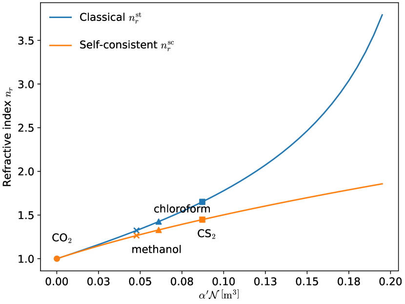
Figure 2: Comparison of classical and self-consistent refractive indices from (63) and (66), respectively, for different molecules at ambient conditions (25^∘ C, 1 bar) calculated from experimental polarizabilities. Notice, under those conditions only CO₂ is gaseous and thus $n_{r}\approx 1$ due to the low number density. Clearly, at increased densities, our relation will eventually break down since the non-overlapping assumption is no longer justified or we would even enter the solid phase, where different physics holds. We have fixed the number density of a molecule for given temperature and pressure via the density $\rho$ as $\mathcal{N}=\frac{N_{A}\rho}{\mathcal{M}}$ ($N_{A}$ is Avogadro’s constant and $\mathcal{M}$ the molar mass).

This implies that changes in the refractive index may be used experimentally to reach for a better mechanistic understanding of VSC. Indeed, measuring the change in refractive index at the same time as the Rabi splitting might allow to determine the effective single-molecular coupling $\lambda$ in parallel with the actual number of molecules contributing to the collective VSC. Notice further, that it is non-trivial to give a precise definition of $\lambda$ in practice and with the associated effective mode volume $\mathcal{V}$ [15].

Finally we investigate the properties of the Tavis-Cummings-type model. Firstly we note that the frequency renormalization would be

$$\omega_{\beta}^{2}\rightarrow\left(1-\frac{(Z_{C}+2Z_{O})^{2}|e|^{2}}{k_{e}\epsilon_{0}\mathcal{V}}\right)\omega_{\beta}^{2}.$$ (68)

Assuming the usual case that the single-particle coupling $\lambda$ is very small, such that the prefactor in Eq. (68) is positive, we have

$$n_{r}^{\rm TC}=\left(1-N_{n}(Z_{C}+2Z_{O})\frac{\alpha}{\epsilon_{0}\mathcal{V}}\right)^{-\tfrac{1}{2}},$$ (69)

where we used Eq. (65) for the case our neutral CO₂ molecule. We immediately note that the Tavis-Cummings-type refractive index does not depend on the number of molecules. That is, the frequency renormalization depends only on a single molecule in a cavity with mode volume $\mathcal{V}$. For the usual case of collective VSC tuned on resonance with the vibrational modes, this effect is expected to be negligibly small. Furthermore, the Tavis-Cummings-type model does not show any change in the vibrational collective mode and so no feedback onto the single molecule from the collective mode besides via the displacement field is expected. This is in agreement with the usual Tavis-Cummings approximation, where the individual molecules remain largely unaffected.

IV Large-$N$ limit and anharmonicities

Let us next comment on the large-$N$ limit. It is clear that even a single molecule in an otherwise empty cavity couples to the mode, i.e., we have a non-zero $\lambda$. We can verify this also by the fact that if we fill a cavity with more and more molecules, we will get a shifted frequency, i.e., we observe a change in refractive index as discussed above. Since for the usual situation of collective strong coupling the number of molecules is very large, while $\lambda$ is very small, a common way to obtain information about this theoretically and numerically challenging case is to fix the Rabi-splitting of the ensemble under investigation and to consider an ersatz problem with less molecules but the same splitting, i.e., one re-scales the coupling as $\lambda(N)=\lambda_{0}/\sqrt{N}$. That is, if we choose $N=1$ we have a single molecule that is strongly-coupled. One can then increase the number of molecules $N$ and consider whether certain properties converge. Following this strategy here, we find with $\gamma^{2}_{0}=N_{n}k_{e}/(N_{n}k_{e}+\lambda_{0}Z_{e})$ and $\tilde{k}_{{\rm a},0}=k_{\rm a}-2\epsilon_{\rm a}\gamma^{2}_{0}\lambda_{0}^{2}$ that

$$\tilde{\omega}_{\beta,0}=\sqrt{N_{n}k_{e}/(N_{n}k_{e}+\lambda_{0}Z_{e})}\,\omega_{\beta}.$$ (70)

That is, besides the Rabi splitting also the red-shift and the frequency change in the collective infrared vibrational mode is fixed to a specific target density $N/\mathcal{V}$. We should, however, be aware that one cannot necessarily take the strict $N\rightarrow\infty$. Indeed, to realize the $N\rightarrow\infty$ limit in the above way, we implicitly increase the effective cavity volume $\mathcal{V}\propto L^{3}\rightarrow\infty$ while increasing the number of molecules. That such a procedure might not only be mathematically problematic but also physically, becomes evident if we remember that we assume the long-wavelength approximation. Thus, all molecules couple instantaneously to the same mode. If these molecules are infinitely far apart this approximation becomes physically unreasonable. This is discussed in more detail in Ref. [15]. Thus if the results do not converge if one reaches the target case $N/\mathcal{V}$ for fixed $N$ and fixed $\mathcal{V}$, the results should be taken with a grain of salt.

Nevertheless, following the above strategy, considering first $\tilde{\rho}_{\rm a}=\rho_{\rm a}/\sqrt{N}$, we find

$$\ddot{\tilde{\rho}}_{{\rm a},0} =-\tilde{k}_{{\rm a},0}\tilde{\rho}_{{\rm a},0}-\frac{2\epsilon_{\rm a}\lambda_{0}}{\omega_{\beta}}\tilde{\omega}^{2}_{\beta,0}q_{\beta,0},$$ (71)

$$\ddot{q}_{\beta,0} =-\tilde{\omega}^{2}_{\beta,0}q_{\beta,0}-\gamma^{2}_{0}\omega_{\beta}\epsilon_{\rm a}\lambda_{0}\tilde{\rho}_{{\rm a},0}.$$ (72)

The property $\tilde{\rho}_{\rm a}$ shows a nice scaling behavior and that the averaged $\tilde{\rho}_{\rm a}$ is well approximated already by a single strongly-coupled molecule. However, if we consider the original $\rho_{\rm a}$ we find a badly scaling

$$\ddot{\rho}_{{\rm a},0} =-\tilde{k}_{{\rm a},0}\rho_{{\rm a},0}-\frac{2\sqrt{N}\epsilon_{\rm a}\lambda_{0}}{\omega_{\beta}}\tilde{\omega}^{2}_{\beta,0}q_{\beta,0},$$ (73)

$$\ddot{q}_{\beta,0} =-\tilde{\omega}^{2}_{\beta,0}q_{\beta,0}-\frac{\gamma^{2}_{0}\omega_{\beta}\epsilon_{\rm a}\lambda_{0}}{\sqrt{N}}\rho_{{\rm a},0},$$ (74)

which suggest potential divergences for large $N$. For instance, if we have a small $q_{\beta,0}$, we will get a diverging external force on $\rho_{{\rm a}}$. On the other hand, if we consider the single-molecule equations we have

$$\ddot{\rho}_{{\rm a},i} =-k_{{\rm a},0}\rho_{{\rm a},i}+\frac{2\epsilon_{\rm a}^{2}\lambda_{0}^{2}\gamma_{0}^{2}}{N}\rho_{{\rm a},0}-\frac{2\epsilon_{\rm a}\lambda_{0}}{\sqrt{N}\omega_{\beta}}\tilde{\omega}^{2}_{\beta,0}q_{\beta,0}.$$ (75)

If we want to recover the frequency shift $\tilde{k}_{{\rm a},0}$ in the collective regime, the collective $\rho_{\rm a}$ has to scale as $N$ and thus diverges. The only way to rectify the collective behavior from a local perspective is to also have a diverging displacement field. This is not a physical problem, since the observable electric field is a sum of both, see Eq. (41). Yet for considering the large-$N$ limit in the above way and making a statement about the local behavior, a purely harmonic model is problematic.

However, things become different, as soon as we allow for anharmonic intra-molecular corrections. We now introduce anharmonic contributions to our bare vibrational CO₂ Hamiltonian up to order $K$ as follows,

$$H^{i,\rm an}_{\rm CO2} = H^{i}_{\rm CO2}+V^{i,\rm an},$$ (76)

$$V^{i,\rm an} = \sum_{\kappa=3}^{K}\frac{\zeta_{\kappa}}{2}\big{[}(R_{i1}-R_{i2})^{\kappa}+(R_{i2}-R_{i3})^{\kappa}\big{]}.$$ (77)

When applying the previously introduced normal mode coordinate transformation, we again find that only the asymmetric vibrational normal mode will couple to the cavity. Moreover, we also find that the translational motion decouples from all anharmonic contributions, thus Eq. (38) remains valid. However, the anharmonicity will introduce mixed local forces terms $F^{\rm an}(\rho_{{\rm a},i},\rho_{{\rm s},i})$ such that

$$\ddot{\rho}_{{\rm s},i} = -k_{\rm s}\rho_{{\rm s},i}+F^{\rm an}_{\rm s}(\rho_{{\rm a},i},\rho_{{\rm s},i}),$$ (78)

$$\ddot{\rho}_{{\rm a},i} = -k_{\rm a}\rho_{{\rm a},i}+F^{\rm an}_{\rm a}(\rho_{{\rm a},i},\rho_{{\rm s},i})$$ (79)

$$+2\epsilon_{\rm a}^{2}\gamma_{0}^{2}\frac{\lambda_{0}^{2}}{N}\rho_{\rm a}-2\epsilon_{\rm a}\gamma_{0}^{2}\frac{\lambda_{0}}{\sqrt{N}}\omega_{\beta}q_{\beta},$$

and the corresponding collective equations become:

$$\ddot{\rho}_{{\rm s}} =-k_{s}\rho_{{\rm s}}-\sum_{i}F^{\rm an}_{\rm s}(\rho_{{\rm a},i},\rho_{{\rm s},i}),$$ (80)

$$\ddot{\rho}_{{\rm a}} =-\tilde{k}_{a}\rho_{{\rm a}}-\sum_{i}F^{\rm an}_{\rm a}(\rho_{{\rm a},i},\rho_{{\rm s},i})$$

$$\qquad-\frac{2\sqrt{N}\epsilon_{\rm a}\lambda_{0}}{\omega_{\beta}}\tilde{\omega}^{2}_{\beta,0}q_{\beta},$$ (81)

$$\ddot{q}_{\beta} =-\tilde{\omega}^{2}_{\beta,0}q_{\beta}-\gamma^{2}_{0}\omega_{\beta}\epsilon_{\rm a}\frac{\lambda_{0}}{\sqrt{N}}\rho_{\rm a}.$$ (82)

Having the additional anharmonic local contributions present allows for collective force cancellation effects to occur on the right side of both Eqs. (81) and (82). Therefore, this setup allows for finite collective forces even with highly correlated molecular motion as indicated by the previous discussion, i.e., $\rho_{a}\propto N$. Allowing for such highly correlated molecular motion in the theoretical description seems vital to accurately capture the local impact of the cavity according to Eq. (79). Putting it differently, the presence of anharmonicities increases the phase space of the collective motion drastically, since the collective motion now explicitly depends on the coordinates of each individual molecule. Therefore, strong correlation or in-phase motion will not necessarily lead to diverging forces anymore.

So far we have not said how correlations between the motion of different molecules could arise. A potential mechanism to correlate the molecular dynamics could be related to the numerically observed formation of a polarization-glass effect, when solving the cavity-Hartree equations for more realistic (anharmonic) electronic structures [10]. In other words, the here-presented anharmonic extension of the harmonic model is still a strong simplification of real molecular systems under VSC. Notice further, that the above anharmonicity argument also holds for the Tavis-Cummings-type approximation, which in principle allows for local strong coupling effects in highly correlated ensembles as well. However, if the dipole-self energy contribution is neglectd, no inter-molecular polarization glass phase can form [10] and thus this mechanism cannot introduce the necessary strong correlations between the molecular vibrations. Nevertheless, our simple argument allows to nicely disentangle the different theoretical mechanisms contributing to VSC. For example, the (many-)electron-nuclear Coulomb interaction of real molecules will give rise to additional anharmonic corrections, caused by the complex electronic structure. Within our model, these electronic contributions are expected to also introduce anharmonic corrections for the dynamics of the displacement-field in Eq. (82). This electronic-structure driven anharmonicity further complicates things (e.g., hyperpolarizabilities will become relevant). In more detail, non-linear transverse electric field corrections can emerge, which will couple to the symmetric modes and even to the center of mass motion of neutral molecules. This will also have interesting consequences in the presence of a thermal bath, which usually affects the translational motions rather than the vibrational modes at ambient conditions. All of which aspects clearly will only be accessible from numerical simulations, which go beyond the scope of this work.

V Conclusion and outlook

Let us collect the results we have obtained from this simple model of collective vibrational strong coupling (VSC). Instead of solving for the wave function of the strongly-coupled ensemble we have considered the equations of motion of the full ensemble. Using the cavity Born-Oppenheimer approximation (cBOA) and that the local single-effective electron wave functions are merely shifted quantum harmonic oscillators, we could find a closed set of equations of motion for the nuclear and displacement coordinates. We could also close the equations for common further approximations employed in polaritonic chemistry, such as ignoring the polarization of matter, i.e., a Tavis-Cummings-type approximation, or using the electronic structure from outside the cavity. We showed that the latter approximation can lead to non-physical results, since the electronic polarization does not fit the nuclear structure and the displacement field of the cavity.

We analyzed this closed set of equations of motion for a harmonic model of an ensemble of CO₂ molecules. Since in this case only $\langle\hat{r}_{i}\rangle$, $\langle\hat{R}_{in}\rangle$ and $\langle\hat{q}_{\beta}\rangle$ appear in the equations of motion, the hierarchy of the usual quantum equations of motion are broken and the classical and quantum equations agree. We find that, in agreement with experiments, only the infrared-active asymmetric vibrational mode couples to the cavity, that the cavity frequency gets red-shifted due to an implicit self-consistent description of the refractive index change when filling the cavity with molecules and that the collective asymmetric mode of the ensemble of molecules is also red-shifted. We have considered how the self-consistent red-shift compares to the usual change in refractive index. We find that up to first order they agree but there can be substantial differences in the higher orders. This might allow to deduce strong-coupling features from changes in the refractive index.

Finally, by considering a simple scaling argument of the coupling, we find that anharmonicities are essential to have a consistent description of the collective and local effects.

While the proposed model sheds some light on potential mechanisms and highlights the necessity of a self-consistent treatment of all the subsystems (electronic, nuclear, displacement) of the ensemble, it is far from ”exact”. Besides the necessity to go beyond the harmonic approximation, we did not touch upon the effect of many (continuum of) modes. Barring mass-renormalization effects [26], the main feature will be to have many weakly coupled modes that lead to further dissipation. That is, these weakly-coupled harmonic oscillators constitute a bath for what the mode+ensemble system is concerned. Of more interest are other strongly enhanced cavity modes. Since this will only add further $q_{\beta}$ terms in the original Hamiltonian, we do not expect large qualitative differences. The main difference that could arise is that we get a strongly red-shifted cavity mode that becomes an efficient thermal pathway, while another one could still be in resonance with the vibrational mode. This could lead to interesting interference effects.

One point that we did not touch upon as well, is the resonance condition observed in experiment. That is, the observed changes seem to rely critically on a matching of energy scales between the cavity mode and a vibrational mode. This effect could be well connected to the potential divergences in our harmonic model in the large-$N$ limit and with this also to the molecular anharmonicities.

All of these aspects make a further detailed investigation of the above simple model and extensions thereof worthwhile.