Duality between controllability and observability
for target control and estimation in networks

Controllability and observability are properties that establish the existence of full-state controllers and observers, respectively. The notions of output controllability and functional observability are generalizations that enable respectively the control and estimation of part of the state vector. These generalizations are of utmost importance in applications to high-dimensional systems, such as large-scale networks, in which only a target subset of variables (nodes) are sought to be controlled or estimated. Although the duality between controllability and observability is well established, the characterization of the duality between their generalized counterparts remains an outstanding problem. Here, we establish both the weak and the strong duality between output controllability and functional observability. Specifically, we show that functional observability of a system implies output controllability of a dual system (weak duality), and that under a certain condition the converse also holds (strong duality). As an application of the strong duality principle, we derive a necessary and sufficient condition for target control via static feedback. This allow us to establish a separation principle between the design of a feedback target controller and the design of a functional observer in closed-loop systems. These results generalize the well-known duality and separation principles in modern control theory.

Keywords: duality principle, separation principle, functional observability, output controllability, target control, geometric approach, static feedback

1 Introduction

Duality is a mathematical concept that enables the solution of one problem to be mapped to the solution of another problem. In modern control theory, the most fundamental example of duality is that between controllability and observability, as introduced by Kalman [1]. Controllability (observability) characterizes the necessary and sufficient condition for the existence of a controller (observer) capable of steering (estimating) the full state of a dynamical system. The duality principle between controllability and observability states that a system is observable if and only if the dual (transposed) system is controllable. When a system is both controllable and observable, the separation principle further establishes that the design of a state feedback controller and of a state observer are mutually independent. The latter facilitates the design of a closed-loop system with feedback from estimated states.

The analysis of controllability and observability has laid a theoretical foundation for full-state controller and observer design, respectively. However, the control and estimation of the entire system state is often unfeasible or not required in high-dimensional systems of current interest, such as large-scale networks [2, 3, 4, 5]. The unfeasibility may arise from physical and/or costs constraints in the placement of actuators and sensors [6, 7] or from a prohibitively high energy required for the operation of these components [8, 9]. These practical limitations led to the development of methods to control and estimate only part of the state vector of the system [10, 11], which subsequently motivated the generalized properties of output controllability [12] and functional observability [13]. Such properties characterize the minimal conditions that enable the control and estimation of pre-specified lower-order functions of the state variables. As a result, these concepts can lead to a substantial order reduction in controller and observer synthesis, as recently demonstrated in target control [14, 15, 16] and target estimation [17, 18] of selected subsets of variables (nodes) in large-scale dynamical networks.

Unlike the concepts of (full-state) controllability and observability [1], output controllability and functional observability emerged in the literature in different contexts and half a century apart [12, 13]. Despite the similarities in purpose, respectively to control and estimate a lower-order function, the existence of a mapping between functional observability of a system and output controllability of another (dual) system is yet to be established. This is the case because the relation between the generalized properties—and between the set of observable and controllable nodes [19]—does not follow straightforwardly from the classical duality principle. For instance, the output controllability of a system does not always imply functional observability of a transposed system (as explicitly shown in Section 2.1). Consequently, algorithms developed for optimal actuator placement in output controllability [14, 15, 20, 21] cannot be employed with guaranteed performance for optimal sensor placement in functional observability [17], and vice versa. This is in contrast with the case of full-state controllability and observability, where a single algorithm can be used to solve both placement problems due to the classical duality principle [22, 23].

In this paper, we establish a duality principle between output controllability and functional observability. Motivated by the notions of weak and strong duality in optimization theory [24, 25], we derive a weak duality between both properties in which the functional observability of a system implies the output controllability of a dual (transposed) system. Moreover, under a specific condition, we establish the strong duality in which the converse also holds. Strong duality leads to the necessary and sufficient conditions for target control via static feedback: when a system is output controllable and its dual system is functionally observable, we show that static feedback control of a linear function of the state variables is possible. Based on these results, we then establish a separation principle in closed-loop systems between the design of a feedback target controller and that of a functional observer. These contributions are shown to be the natural extensions of the classical duality and separation principles in modern control theory.

The paper is organized as follows. Section 2 reviews the notions of output controllability and functional observability. Sections 3 and 4 present our main results, respectively establishing the duality and separation principles between the generalized notions of controllability and observability. Section 5 summarizes our contributions and discusses opportunities for future research.

2 Preliminaries

Consider the linear time-invariant dynamical system

$$\dot{\bm{x}} =A\bm{x}+B\bm{u},$$ (1)

$$\bm{y} =C\bm{x},$$ (2)

where $\bm{x}\in\mathbb{R}^{n}$ is the state vector, $\bm{u}\in\mathbb{R}^{p}$ is the input vector, $\bm{y}\in\mathbb{R}^{q}$ is the output vector, $A\in\mathbb{R}^{n\times n}$ is the system matrix, $B\in\mathbb{R}^{n\times p}$ is the input matrix, and $C\in\mathbb{R}^{q\times n}$ is the output matrix. By convention, we use $(A,B)$ to analyze the controllability of a system with system matrix $A$ and input matrix $B$, and $(C,A)$ to analyze the observability of a system with output matrix $C$ and system matrix $A$. The linear function of the state variables

$$\bm{z}=F\bm{x}$$ (3)

defines the target vector $\bm{z}\in\mathbb{R}^{r}$ sought to be controlled or estimated, where $F\in\mathbb{R}^{r\times n}$ is the functional matrix ($r\leq n$).

Let the output controllable set $\mathcal{C}_{F}$ of a system (1)–(3) be the set of all reachable states $\bm{z^{*}}\in\mathbb{R}^{r}$ for which there exists an input $\bm{u}(t)$ that steers the system from an initial state $\bm{x}(0)={0}$ to some final state $\bm{x}(t_{1})$ in finite time $t\in[0,t_{1}]$ such that $\bm{z}(t_{1})=F\bm{x}(t_{1}):=\bm{z}^{*}$. The system represented by the triple $(A,B;F)$ is output controllable when the set $\mathcal{C}_{F}$ is $\mathbb{R}^{r}$. A necessary and sufficient condition for output controllability is [12, 26]

$$\operatorname{rank}(F\mathcal{C})=\operatorname{rank}(F),$$ (4)

where $\mathcal{C}=[B\,\,AB\,\,A^{2}B\,\,\ldots\,\,A^{n-1}B]$ is the controllability matrix. In particular, condition (4) is necessary and sufficient for the invertibility of $FW_{c}(t_{1})F^{\mathsf{T}}$ [27, Section 9.6], hence guaranteeing that, for each $\bm{z^{*}}\in\mathcal{C}_{F}$, there exists a control law

$$\bm{u}(t)=B^{\mathsf{T}}e^{A^{\mathsf{T}}(t_{1}-t)}F^{\mathsf{T}}(FW_{c}(t_{1})F^{\mathsf{T}})^{-1}\bm{z}^{*}$$ (5)

capable of steering the target vector from $\bm{z}(0)={0}$ to $\bm{z}(t_{1})=\bm{z^{*}}$, where $W_{c}(t)=\int_{0}^{t}e^{A(t-\tau)}BB^{\mathsf{T}}e^{A^{\mathsf{T}}(t-\tau)}\text{d}\tau$ is the controllability Gramian.

Remark 1.

The nomenclature “output controllability” was originally motivated by applications in which the target vector $\bm{z}(t)$ sought to be controlled was precisely the output $\bm{y}(t)$ (i.e., $F=C$) [12, 28, 26]. However, this property can be defined more generally for any $F$ as presented above. This led to the notion of “partial stability and control” for linear and nonlinear systems [11, 29], as well as the more contemporaneous terminology “target controllability” in graph-theoretical studies in which only a subset of variables (nodes) are sought to be controlled [14, 15, 20, 21, 30, 31].

In addition, let the functionally observable set $\mathcal{O}_{F}$ of system (1)–(3) be the set of all $\bm{z}^{*}\in\mathbb{R}^{r}$ such that the initial condition $\bm{z}(0)=F\bm{x}(0):=\bm{z}^{*}$ can be uniquely determined from the output $\bm{y}(t)$ and input $\bm{u}(t)$ signals over $t\in[0,t_{1}]$. The system represented by the triple $(C,A;F)$ is functionally observable when the set $\mathcal{O}_{F}$ is $\mathbb{R}^{r}$. A necessary and sufficient condition for functional observability is

$$\operatorname{rank}\left(\begin{bmatrix}\mathcal{O}\\ F\end{bmatrix}\right)=\operatorname{rank}(\mathcal{O}),$$ (6)

where $\mathcal{O}=[C^{\mathsf{T}}\,\,(CA)^{\mathsf{T}}\,\,(CA^{2})^{\mathsf{T}}\,\,\ldots\,\,(CA^{n-1})^{\mathsf{T}}]^{\mathsf{T}}$ is the observability matrix (see proof of this result in [32, Theorem 5] and [33, Section I]). Indeed, condition (6) is necessary and sufficient for the existence of some matrix $G\in\mathbb{R}^{r\times n}$ such that $GW_{o}(t_{1})=F$, guaranteeing the reconstruction of the initial condition in finite time [17]. That is,

$$W_{o}(t_{1})\bm{x}(0) =\int_{0}^{t_{1}}e^{A^{\mathsf{T}}t}C^{\mathsf{T}}\bm{h}(t,\bm{u},\bm{y})\text{d}t$$ (7)

$$\text{implies}\quad\bm{z}(0) =G\int_{0}^{t_{1}}e^{A^{\mathsf{T}}t}C^{\mathsf{T}}\bm{h}(t,\bm{u},\bm{y})\text{d}t,$$ (8)

where $\bm{h}(t,\bm{u},\bm{y})=\bm{y}(t)-C\int_{0}^{t}e^{-A\tau}\bm{B}\bm{u}(\tau){\rm d}\tau$ is a functional of the system input $\bm{u}(t)$ and output $\bm{y}(t)$ over $t\in[0,t_{1}]$, and $W_{o}(t)=\int_{0}^{t}e^{A^{\mathsf{T}}\tau}C^{\mathsf{T}}Ce^{A\tau}{\rm d}\tau$ is the observability Gramian.

Remark 2.

If all state variables are sought to be controlled or estimated (i.e., $F=I_{n}$, where $I_{n}$ is the identity matrix of size $n$), then conditions (4) and (6) reduce, respectively, to the classical conditions of full-state controllability ($\operatorname{rank}(\mathcal{C})=n$) and full-state observability ($\operatorname{rank}(\mathcal{O})=n$).

Throughout, we use $(A,B;F)$ to analyze the output controllability of a system with system matrix $A$, input matrix $B$, and functional matrix $F$, and we use the terminology “target control” to refer to the control of the target vector $\bm{z}(t)$ via an input signal $\bm{u}(t)$. Likewise, we use $(C,A;F)$ to analyze the functional observability of a system with output matrix $C$, system matrix $A$, and functional matrix $F$, and we use “target estimation” to refer to the estimation of the target vector $\bm{z}(t)$ from an output signal $\bm{y}(t)$. The following assumption is considered in this paper.

Assumption 1.

The functional matrix has linearly independent rows (i.e., $\rank(F)=r$).

This assumption guarantees that an output controllable system can drive independently every component $\bm{z}_{i}(t)$ of the target vector to any arbitrary final state $\bm{z}_{i}^{\star}$. In the functional observability problem, this assumption is made without loss of generality given that $\bm{z}^{\prime}:=F^{\prime}\bm{x}=\bm{\gamma}^{\mathsf{T}}\bm{z}$ for some $\bm{\gamma}\in\mathbb{R}^{r}$ and any $F^{\prime}$ that is a linear combination of the rows of $F$. Thus, $\bm{z}^{\prime}$ can be inferred from $\bm{z}$, which in turn is uniquely determined by $\bm{y}$ if and only if $(C,A;F)$ is functionally observable.

2.1 Example

We show that output controllability and functional observability are not always directly related by a system transposition, in contrast with the classical duality between full-state controllability and observability. Consider a dynamical system (1)–(3) given by

$$A=\begin{bmatrix}0&0&0\\ 1&0&0\\ 1&0&0\\ \end{bmatrix},\quad B=\begin{bmatrix}1\\ 0\\ 0\end{bmatrix},\quad F=\begin{bmatrix}0&1&0\end{bmatrix}.$$ (9)

The system $(A,B)$ is uncontrollable and, by duality, $(B^{\mathsf{T}},A^{\mathsf{T}})$ is unobservable. Given that $\rank(F\mathcal{C})=\rank(F)=1$, the system $(A,B;F)$ is output controllable. On the other hand, the transposed system $(B^{\mathsf{T}},A^{\mathsf{T}};F)$ is not functionally observable since $\rank[\mathcal{O}^{\mathsf{T}}\,\,F^{\mathsf{T}}]^{\mathsf{T}}=3>2=\rank(\mathcal{O})$.

3 Duality Principle

We now generalize the concept of duality between controllability and observability. Consider a pair of systems $(C,A;F)$ and $(A^{\mathsf{T}},C^{\mathsf{T}};F)$. We show that the functional observability of the former is in general a sufficient (but unnecessary) condition for the output controllability of the latter. This result will thus establish the weak duality between functional observability and output controllability. By further imposing a certain condition on the system matrices, the functional observability of $(C,A;F)$ becomes equivalent to the output controllability of $(A^{\mathsf{T}},C^{\mathsf{T}};F)$, which we call the strong duality.

In what follows, let $\mathcal{O}_{F}$ be the functionally observable set of the system $(C,A;F)$ and $\mathcal{C}_{F}$ be the output controllable set of the dual system $(A^{\mathsf{T}},C^{\mathsf{T}};F)$. Given any final time $t_{1}$, the observability Gramian of system $(C,A)$ and the controllability Gramian of system $(A^{\mathsf{T}},C^{\mathsf{T}})$ coincide, and we denote it by $W=\int_{0}^{t_{1}}e^{A^{\mathsf{T}}\tau}C^{\mathsf{T}}Ce^{A\tau}d\tau$. Let $W=U\Lambda U^{H}$ be the eigendecomposition of the symmetric matrix $W$, where $\Lambda$ is the diagonal of eigenvalues and $U$ is the unitary matrix of eigenvectors. We partition $U$ into $U=[U_{1}\,\,\,U_{2}]$, where $U_{1}$ and $U_{2}$ consist of columns corresponding to nonzero and zero eigenvalues, respectively. Clearly, $W=U_{1}\Lambda_{1}U_{1}^{H}$, where $\Lambda_{1}$ is the diagonal matrix of nonzero eigenvalues. We have that $\operatorname{Im}(W)=\operatorname{Im}(U_{1})$ and $\operatorname{Ker}(W)=\operatorname{Im}(U_{2})$.

Theorem 1 (Weak duality).

For any given pair of systems $(C,A;F)$ and $(A^{\mathsf{T}},C^{\mathsf{T}};F)$, the relation $\mathcal{O}_{F}\subseteq\mathcal{C}_{F}$ holds. Therefore, if $(C,A;F)$ is functionally observable, then $(A^{\mathsf{T}},C^{\mathsf{T}};F)$ is output controllable.

Proof.

According to [34, Theorem 2.2], the set of reachable states of system $(A^{\mathsf{T}},C^{\mathsf{T}};F)$ is equal to the image set of the controllability Gramian $\operatorname{Im}(W)$. Therefore, $\mathcal{C}_{F}=F\operatorname{Im}(W)$. For system $(C,A;F)$, consider Eq. (7), which is equivalent to

$$U_{1}^{H}\bm{x}(0)=\Lambda_{1}^{-1}U_{1}^{H}\int_{0}^{t_{1}}e^{A^{\mathsf{T}}t}C^{\mathsf{T}}\bm{h}(t,\bm{u},\bm{y})\text{d}t.$$ (10)

Thus, $\bm{z}(0)=F\bm{x}(0)=FU_{1}U_{1}^{H}\bm{x}(0)+FU_{2}U_{2}^{H}\bm{x}(0)$, yielding

$$\bm{z}(0)= \,\,FU_{1}\Lambda_{1}^{-1}U_{1}^{H}\int_{0}^{t_{1}}e^{A^{\mathsf{T}}t}C^{\mathsf{T}}\bm{h}(t,\bm{u},\bm{y})\text{d}t$$ (11)

$$+FU_{2}U_{2}^{H}\bm{x}(0).$$

Since the initial condition $\bm{x}(0)$ is arbitrary and unknown, it follows from Eq. (11) that $\bm{z}(0)$ can be uniquely determined by the (known) functional $\bm{h}(t,\bm{u},\bm{y})$ of the system input and output only if $FU_{2}U_{2}^{H}\bm{x}(0)=0$, which is equivalent to the condition $\bm{z}(0)\perp F\operatorname{Im}(U_{2})$. It thus follows from Eq. (11) that the necessary and sufficient condition for $\bm{z}(0)$ to be uniquely determined from $\bm{h}(t,\bm{u},\bm{z})$ is that $\bm{z}(0)\perp F\operatorname{Im}(U_{2})$ and $\bm{z}(0)\in F\operatorname{Im}(U_{1})$. Consequently,

$$\mathcal{O}_{F}=\operatorname{Im}(FU_{1})\cap(F\operatorname{Im}(U_{2}))^{\perp}=\mathcal{C}_{F}\cap(F\operatorname{Ker}(W))^{\perp}.$$ (12)

It follows that $\mathcal{O}_{F}\subseteq\mathcal{C}_{F}$. If $(C,A;F)$ is functionally observable, then $\mathcal{O}_{F}=\mathbb{R}^{r}$ and hence $\mathcal{C}_{F}=\mathbb{R}^{r}$. Thus, by definition, $(A^{\mathsf{T}},C^{\mathsf{T}};F)$ is output controllable. ∎

Theorem 2 (Strong duality).

For any given pair of systems $(C,A;F)$ and $(A^{\mathsf{T}},C^{\mathsf{T}};F)$, the relation $\mathcal{O}_{F}=\mathcal{C}_{F}$ holds if and only if $F\operatorname{Im}(W)\perp F\operatorname{Ker}(W)$. Under this condition, $(C,A;F)$ is functionally observable if and only if $(A^{\mathsf{T}},C^{\mathsf{T}};F)$ is output controllable.

Proof.

According to Eq. (12), $\mathcal{O}_{F}=\mathcal{C}_{F}$ if and only if $\mathcal{C}_{F}\subseteq(F\operatorname{Ker}(W))^{\perp}$, which is equivalent to $F\operatorname{Im}(W)\perp F\operatorname{Ker}(W)$. Moreover, if $\mathcal{C}_{F}=\mathcal{O}_{F}=\mathbb{R}^{r}$, then by definition $(C,A;F)$ is functionally observable and $(A^{\mathsf{T}},C^{\mathsf{T}};F)$ is output controllable. ∎

Remark 3.

Theorems 1 and 2 provide a geometric characterization of the generalized duality in terms of the inclusion relation between the output controllable set $\mathcal{C}_{F}$ and the functionally observable set $\mathcal{O}_{F}$. We can define the duality gap as $\gamma=\operatorname{dim}(\mathcal{C}_{F})-\operatorname{dim}(\mathcal{O}_{F})\geq 0$. The strong duality holds if and only if $\gamma=0$.

Remark 4.

Theorem 2 generalizes the classical duality principle between full-state controllability and observability [35, Theorem 6.5]. To see this, note that for $F=I_{n}$ the condition in Theorem 2 reduces to $\operatorname{Im}(W)\perp\operatorname{Ker}(W)$, which holds for any symmetric matrix $W$. Thus, $\mathcal{O}_{I_{n}}=\mathcal{C}_{I_{n}}$, $\gamma=0$, and the observability of $(C,A;I_{n})$ implies and is implied by the controllability of $(A^{\mathsf{T}},C^{\mathsf{T}};I_{n})$.

Remark 5.

The geometric relation (12) between the sets $\mathcal{O}_{F}$ and $\mathcal{C}_{F}$ has a direct interpretation in the geometric approach to control theory [36, 37]. It follows from condition (4) that the triple $(A,B;F)$ is output controllable if and only if $F\langle A|\imaginary(B)\rangle=\mathbb{R}^{r}$ [38], where the controllable subspace $\langle A|\imaginary(B)\rangle=\imaginary(B)+A\imaginary(B)+\ldots+A^{n-1}\imaginary(B)$ is the smallest $A$-invariant subspace containing $\imaginary(B)$. Likewise, it follows from condition (6) that $(C,A;F)$ is functionally observable if and only if $\imaginary(F^{\mathsf{T}})\cap\mathcal{N}=\{0\}$, where the unobservable subspace $\mathcal{N}=\bigcap_{i=0}^{n-1}\operatorname{Ker}(CA^{i})$ is the largest $A$-invariant subspace contained in $\operatorname{Ker}(C)$. For a pair of dual systems $(C,A;F)$ and $(A^{\mathsf{T}},C^{\mathsf{T}};F)$, we have $\mathcal{N}=\langle A^{\mathsf{T}}|\operatorname{Im}(C^{\mathsf{T}})\rangle^{\perp}$. From the duality principle, it follows that $\imaginary(F^{\mathsf{T}})\cap\mathcal{N}=\{0\}$ implies $F\mathcal{N}^{\perp}=\mathbb{R}^{r}$ and the converse holds if and only if $F\mathcal{N}^{\perp}\perp F\mathcal{N}$.

Figure 1: Diagram of the established duality principle between functional observability and output controllability. Solid arrows indicate that a given property implies another while dashed arrows indicate that a property implies the other under certain conditions.

Fig. 1 illustrates the relation between the output controllable space $\mathcal{C}_{F}$ and the functional observable space $\mathcal{O}_{F}$ of a pair of systems. When $\mathcal{C}_{F}=\mathbb{R}^{r}$ and/or $\mathcal{O}_{F}=\mathbb{R}^{r}$ holds, this relation leads to the weak and strong duality principles between the output controllability and functional observability properties, as well as the classical cases for $F=I_{n}$. Strong duality may hold even if the two systems are neither output controllable nor functionally observable (e.g., the trivial case where $C=0$ and $W=0$, and hence $F\operatorname{Im}(0)\perp F\operatorname{Ker}(0)$). On the other hand, strong duality always holds if a system is functionally observable, but not necessarily if the system is output controllable. The following corollaries provide sufficient conditions for the strong duality principle.

Corollary 1.

A pair of systems $(C,A;F)$ and $(A^{\mathsf{T}},C^{\mathsf{T}};F)$ is strongly dual (i.e., $\mathcal{O}_{F}=\mathcal{C}_{F}$) if the rank condition (6) is satisfied for the system $(C,A;F)$.

Proof.

If condition (6) is satisfied, then $\operatorname{row}(F)\subseteq\operatorname{row}(\mathcal{O})$ and $F\operatorname{Ker}(\mathcal{O})=\{0\}$. Since $\operatorname{Im}(W)=\operatorname{Im}(\mathcal{O})$, it follows that the strong duality condition in Theorem 2 holds trivially. ∎

Corollary 2.

A pair of systems $(C,A;F)$ and $(A^{\mathsf{T}},C^{\mathsf{T}};F)$ is strongly dual if $\bm{z}=F\bm{x}$ is a conformal linear transformation.

Proof.

By definition, $F$ represents a conformal linear transformation if and only if the transformation preserves the angles between any two vectors, and thus $\frac{\langle\bm{x},\tilde{\bm{x}}\rangle}{|\bm{x}||\tilde{\bm{x}}|}=\frac{\langle F\bm{x},F\tilde{\bm{x}}\rangle}{|F\bm{x}||F\tilde{\bm{x}}|}$ for all $\bm{x},\tilde{\bm{x}}\in\mathbb{R}^{n}$. Since $\imaginary(W)\perp\operatorname{Ker}(W)$, the orthogonality $F\imaginary(W)\perp F\operatorname{Ker}(W)$ is preserved. ∎

3.1 Example

Consider the 5-dimensional dynamical system given by

$$A=\begin{bmatrix}-1&0&0&0&-1\\ -1&a_{22}&0&0&0\\ 0&0&a_{33}&0&0\\ 0&0&0&a_{44}&0\\ 0&-1&-1&-1&-1\end{bmatrix},\quad C=\begin{bmatrix}0&0&0&0&1\end{bmatrix},$$ (13)

and the target vector (3) defined by

$$F=\begin{bmatrix}0&1&0&0&0\end{bmatrix}.$$ (14)

Let $a_{22}\neq 0$ and $a_{33}=a_{44}=0$ except when stated otherwise. Fig. 2a provides a graph representation of this system. The observability matrix corresponding to the pair $(C,A)$ is thus given by

$$\mathcal{O}=\footnotesize\left[\begin{array}[]{*{5}{c@{\hspace{4pt}}}}0\hfil\hskip 4.0&0\hfil\hskip 4.0&0\hfil\hskip 4.0&0\hfil\hskip 4.0&1\hfil\hskip 4.0\\ 0\hfil\hskip 4.0&-1\hfil\hskip 4.0&-1\hfil\hskip 4.0&-1\hfil\hskip 4.0&-1\hfil\hskip 4.0\\ 1\hfil\hskip 4.0&-a_{22}+1\hfil\hskip 4.0&1\hfil\hskip 4.0&1\hfil\hskip 4.0&1\hfil\hskip 4.0\\ a_{22}-2\hfil\hskip 4.0&-a_{22}^{2}+a_{22}-1\hfil\hskip 4.0&-1\hfil\hskip 4.0&-1\hfil\hskip 4.0&-2\hfil\hskip 4.0\\ a_{22}^{2}-2a_{22}+3\hfil\hskip 4.0&-a_{22}^{3}+a_{22}^{2}-a_{22}+2\hfil\hskip 4.0&2\hfil\hskip 4.0&2\hfil\hskip 4.0&-a_{22}+4\hfil\hskip 4.0\end{array}\right].$$ (15)

The system is unobservable given that $\operatorname{rank}(\mathcal{O})<5$. However, the system is still functionally observable with respect to the functional (14) since $\operatorname{row}(F)\subseteq\operatorname{row}(\mathcal{O})$, hence satisfying condition (6). Thus, although it is not possible to reconstruct the full-state vector $\bm{x}=[x_{1},\,\,\ldots\,\,x_{5}]^{\mathsf{T}}$ from measurements $\bm{y}(t)=x_{5}(t)$ over $t\in[0,t_{1}]$, the target variable $\bm{z}=x_{2}$ can be reconstructed in finite time.

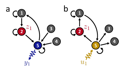
Figure 2: Graph representation of a dual pair of dynamical systems. (a) System $(C,A;F)$, defined by matrices (13) and (14). (b) Dual system $(A^{\mathsf{T}},C^{\mathsf{T}};F)$. In each system, nodes represent the state variables $\{x_{1},\ldots,x_{n}\}$ and an edge connecting node $j$ to node $i$ represents the nonzero entry $a_{ij}$ in the system matrix $A$. Note that transposing $A$ in the dual system is equivalent to reversing the direction of the corresponding edges linking two nodes. The input, output, and target variables are highlighted by yellow, blue, and red nodes, respectively.

Consider now the dual system to (13) given by the transposed system matrix $A^{\mathsf{T}}$ and an input matrix $B=C^{\mathsf{T}}$, as illustrated by the graph representation in Fig. 2b. The weak duality principle (Theorem 1) establishes that, since the system $(C,A;F)$ is functionally observable, the dual system $(A^{\mathsf{T}},C^{\mathsf{T}};F)$ is necessarily output controllable. This can be directly checked by computing the controllability matrix of $(A^{\mathsf{T}},C^{\mathsf{T}})$, given by $\mathcal{C}=\mathcal{O}^{\mathsf{T}}$, and verifying that condition (4) is satisfied.

The converse relation, however, is not always true: output controllability of the dual system is not sufficient for the functional observability of the original system. By considering $a_{22}=0$ (equivalent to the absence of a self-edge in node 2 in Fig. 2), the dual system $(A^{\mathsf{T}},C^{\mathsf{T}};F)$ remains output controllable (i.e., $\operatorname{rank}([0\,\,-1\,\,1\,\,-1\,\,2])=\operatorname{rank}(F)$), although the original system $(C,A;F)$ loses functional observability (i.e., $\operatorname{row}(F)\nsubseteq\operatorname{row}(\mathcal{O})$). This follows from the properties of the controllable and observable spaces defined by the Gramian $W$, as we show next. First, recall that $\operatorname{Im}(W)=\operatorname{Im}(\mathcal{O})=\operatorname{Im}(\mathcal{C}^{\mathsf{T}})$. From Eq. (15), for $a_{22}=0$ it follows that

$$F\operatorname{Im}(W) =\operatorname{span}\{\begin{bmatrix}0&1&0&-1&1\end{bmatrix}\},$$ (16)

$$F\operatorname{Ker}(W) =\operatorname{span}\{\begin{bmatrix}0&2&-1&-1&0\end{bmatrix}\}.$$ (17)

Since the subspaces $F\operatorname{Im}(W)$ and $F\operatorname{Ker}(W)$ are not orthogonal, the condition for strong duality (Theorem 2) is not satisfied and the original system $(C,A;F)$ is not functionally observable. Indeed, strong duality is possible only if $a_{22}\neq 0$, where $F\operatorname{Ker}(W)=\{0\}$ and thus $F\operatorname{Im}(W)\perp F\operatorname{Ker}(W)$.

3.2 Target control and observation energy in networks

In applications to large-scale networks, testing the output controllability and functional observability of a system using the algebraic rank conditions (4) and (6), respectively, can be prone to numerical challenges due to the poor conditioning of the controllability and observability matrices for large $n$. To circumvent these challenges, generic notions of output controllability [15, 20, 21, 30, 31] and functional observability [17] for structured systems have been proposed in the literature. These previous studies established intuitive graph-theoretic conditions based on the network structure, the set of actuators (or sensors), and the set of targets—respectively encoded by matrices $A$, $B$ (or $C$), and $F$. The structural approach has led to efficient algorithms for the minimum placement of actuators and sensors in large-scale networks, and is suitable for systems involving modeling uncertainties in the parameters (when the structure of $A$ is reliably known but the exact numerical entries are not).

We have recently investigated the output controllability and functional observability problems from a structural viewpoint [39]. This allowed us to leverage duality to repurpose existing algorithms for minimum actuator/sensor placement to address previously unsolved problems. In addition to establishing that the output controllability and functional observability of a system can be reliably tested, it is important to address the question of how “hard” it is to control or observe the target vector $\bm{z}(t)$. For practical purposes, and in accordance with the existing literature [6, 40, 41, 7, 16], we measure this hardness in terms of energy. We propose the following measures of the control (observation) energy required to drive (observe) a target vector.

Target control energy. Consider an output controllable system $(A,B;F)$. Let the control signal $\bm{u}(t)$ be determined by Eq. (5), which is the control law that requires the smallest amount of energy $\int_{0}^{t_{1}}\norm{\bm{u}(t)}^{2}{\rm d}t$ in order to drive a target vector from the initial state $\bm{z}(0):=F\bm{x}(0)=0$ to a given final state $\bm{z}^{*}:=F\bm{x}^{*}$, where $\bm{x}^{*}:=\bm{x}(t_{1})$. We refer to $\bm{z}^{*}$ for which the minimum energy is the largest as the worst-case scenario and the corresponding energy as the maximum target control energy [16]:

$$E_{\rm tc}:=\max_{\norm{F\bm{x}^{*}}=1}\int_{0}^{t_{1}}\norm{\bm{u}(t)}^{2}{\rm d}t=\frac{1}{\lambda_{\rm min}(FW_{c}F^{\mathsf{T}})},$$ (18)

where $\lambda_{\rm min}(\cdot)$ denotes the minimum eigenvalue of a matrix. This expression can be derived by considering Eq. (5) for the initial state $\bm{x}(0)=0$, which leads to

$$\int_{0}^{t_{1}}\norm{\bm{u}(t)}^{2}{\rm d}t =(\bm{z}^{*})^{\mathsf{T}}(FW_{c}F^{\mathsf{T}})^{-1}\bm{z}^{*}$$ (19)

$$\leq\lambda_{\rm max}\left((FW_{c}F^{\mathsf{T}})^{-1}\right)\norm{\bm{z}^{*}}.$$

If the system is not output controllable, then $FWF^{\mathsf{T}}$ is singular and thus the optimal control energy $\int_{0}^{t_{1}}\norm{\bm{u}(t)}^{2}{\rm d}t$ is undefined. This possibility is accounted for by Eq. (18) since $\lambda_{\rm min}(FWF^{\mathsf{T}})=0$ and hence target control is unfeasible in this case (i.e., $E_{\rm tc}=\infty$).

Target observation energy. Consider a functionally observable system $(C,A;F)$. We now propose a measure of the energy contribution to the output signal that comes from the (initial) target state $\bm{z}^{*}:=F\bm{x}^{*}$ to be observed, where here $\bm{x}^{*}:=\bm{x}(0)$ denotes the initial state. For the worst-case scenario, we call this measure the minimum target observation energy and express it as

$$E_{\rm to}:=\min_{\norm{F\bm{x}^{*}}=1}\int_{0}^{t_{1}}\norm{\bm{y}(t)}^{2}{\rm d}t=\frac{1}{\lambda_{\rm max}(FW_{o}^{\dagger}F^{\mathsf{T}})},$$ (20)

where we assumed that the matrix $A$ is Hurwitz stable so that the output signal is bounded. Small values of $E_{\rm to}$ imply small contributions of $\bm{z}^{*}$ to the output energy $\int_{0}^{t_{1}}\norm{\bm{y}(t)}^{2}{\rm d}t$, which may be obscured by practical factors (e.g., noise and numerical errors) and in turn compromise the target estimation accuracy.

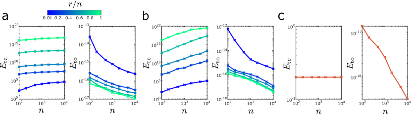
Figure 3: Target control energy $E_{\rm tc}$ and target observation energy $E_{\rm to}$ as a function of the network size $n$ in (a) scale-free networks, (b) small-world networks, and (c) chain networks. Each data point represents the average energy across 100 independent realizations of the network models. For each realization, the state variables $\bm{x}_{i}$ representing nodes in the network are actuated independently in the left panel (i.e., $B\in\mathbb{R}^{n\times p}$ has only one nonzero entry per column) and measured independently in the right panel (i.e., $C\in\mathbb{R}^{q\times n}$ has only one nonzero entry per row). In (a) and (b), the target variables are also selected independently (i.e., $F\in\mathbb{R}^{r\times n}$ has only one nonzero entry per row), and the nonzero entries of $F$, $B$, and $C$ are selected randomly. The curves are color coded according to the fraction of target nodes $r/n$, for $p=q=0.1n$. In (c), we set $p=q=r=1$, where only the first node is actuated in the left panel (i.e., $B=[1\,\,0\,\,0\,\,\ldots\,\,0]^{\mathsf{T}}$) and measured in right panel (i.e., $C=B^{\mathsf{T}}$). The target variable is defined as $z=\sum_{i=1}^{n}x_{i}$ (i.e., $F=[1\,\,1\,\,1\,\,\ldots\,\,1]$). In all simulations, the Gramian $W$ is computed using the system matrix $A=-(L+\alpha I_{n})$, where $L$ represents the Laplacian matrix of the (symmetric) adjacency matrix $G$, $\alpha=0.1$ is set to ensure numerical stability of the matrices for large systems, and $G_{ij}\sim\mathcal{U}[0,1]$ if node $j$ is connected to $i$ and $G_{ij}=0$ otherwise. The scale-free networks were generated using the Barabási–Albert model [42], where each new node is preferentially attached to 3 existing nodes, and the small-world networks were generated using the Newman–Watts model [43], where the probability of adding a new edge to a ring graph is 0.2.

To solve the optimization problem (20), consider the Lagrangian function $\mathcal{L}(\bm{x}^{*},\lambda)=\int_{0}^{t_{1}}\norm{\bm{y}(t)}^{2}{\rm d}t+\lambda(\norm{F\bm{x}^{*}}^{2}-1)$, where $\lambda$ is the Lagrangian multiplier and $\int_{0}^{t_{1}}\norm{\bm{y}(t)}^{2}{\rm d}t=(\bm{x}^{*})^{\mathsf{T}}W_{o}\bm{x}^{*}$. The critical points $({\bm{x}}^{*},{\lambda})$ of $\mathcal{L}$ are thus given by

$$\gradient_{\bm{x}^{*}}\mathcal{L}(\bm{x}^{*},\lambda)=(W_{o}-\lambda F^{\mathsf{T}}F){\bm{x}}^{*}=0.$$ (21)

Evaluating the cost function at these critical points yields $\int_{0}^{t_{1}}\norm{\bm{y}(t)}^{2}{\rm d}t=({\bm{x}}^{*})^{\mathsf{T}}W_{o}{\bm{x}}^{*}=({\bm{x}}^{*})^{\mathsf{T}}\lambda F^{\mathsf{T}}F{\bm{x}}^{*}=\lambda\norm{F{\bm{x}}^{*}}^{2}=\lambda$, where we imposed the constraint $\norm{F\bm{x}^{*}}=1$. From (21), it follows that the Lagrangian multiplier $\lambda$ is an eigenvalue of the matrix pencil $W_{o}-\lambda F^{\mathsf{T}}F$, also denoted $(W_{o},F^{\mathsf{T}}F)$. Therefore, $E_{\rm to}=\lambda_{\rm min}(W_{o},F^{\mathsf{T}}F)$, which is the smallest eigenvalue of the matrix pencil $(W_{o},F^{\mathsf{T}}F)$. Multiplying Eq. (21) on the left by $G$ and recalling that $GW_{o}=F$, we obtain

$$\left(GF^{\mathsf{T}}-\frac{1}{\lambda}I_{r}\right)\bm{z}_{0}=0.$$ (22)

This implies that $E_{\rm to}=\lambda_{\rm min}(W_{o},F^{\mathsf{T}}F)=\left[\lambda_{\rm max}(GF^{\mathsf{T}})\right]^{-1}$, where $G=FW_{o}^{\dagger}$ and $W_{o}^{\dagger}$ denotes the right pseudoinverse of $W_{o}$ (i.e., $W_{o}W_{o}^{\dagger}=I_{n}$). Note that if the system is not functionally observable, there does not exist a matrix $G$ such that $GW_{o}=F$ and hence $E_{\rm to}$ is undefined.

Remark 6.

By imposing the constraint $\norm{F\bm{x}^{*}}=1$, the worst-case energies in Eqs. (18) and (20) correspond to the directions in the row space of $F$ that are the hardest to control and observe, respectively. For the special case of $F=I_{n}$, the target control energy reduces to the worst-case controllability measure $E_{\rm tc}=\left[\lambda_{\rm min}(W_{c})\right]^{-1}$ studied in past work on full-state control [6, 40, 7]; similarly, the target observation energy reduces to $E_{\rm to}=\left[\lambda_{\rm max}(W_{o}^{-1})\right]^{-1}=\lambda_{\rm min}(W_{o})$.

Remark 7.

For a pair of dual systems, the controllability and observability Gramians are equal ($W_{c}=W_{o}=:W$) but the energy measures $E_{\rm tc}$ and $E_{\rm to}$ are not directly related in general. As a special case, when $F$ has orthonormal columns (i.e., $F^{\mathsf{T}}F=I_{n}$), it follows that $F^{\mathsf{T}}=F^{\dagger}$ and $FW^{\dagger}F^{\mathsf{T}}=(F^{\mathsf{T}})^{\dagger}W^{\dagger}F^{\dagger}=(FWF^{\mathsf{T}})^{\dagger}$. By assumption, $E_{\rm tc}$ ($E_{\rm to}$) is defined for output controllable (functionally observable) systems. Therefore, $FWF^{\mathsf{T}}$ is nonsingular and $(FWF^{\mathsf{T}})^{\dagger}=(FWF^{\mathsf{T}})^{-1}$, yielding the relation $E_{\rm to}=E_{\rm tc}^{-1}$. This example suggests that the degree of difficulty to observe a system $(C,A;F)$ goes hand in hand with the difficulty to control the dual system $(A^{\mathsf{T}},C^{\mathsf{T}};F)$. However, such a simple relation is not expected for a general pair of dual systems, as illustrated below.

Example. Fig. 3a,b presents the scaling of the target energy measures for scale-free and small-world networks of increasing size. The target control (observation) energy increases (decreases) on average with the network size $n$. As expected, the rate of increase depends on the underlying network structure as well as the proportion of target variables. Since the control and output energy are limited in practical applications, it is usually unfeasible to control (reconstruct) the target state of networks associated with small (large) eigenvalues of $FW_{c}F^{\mathsf{T}}$ ($FW_{o}^{\dagger}F^{\mathsf{T}}$). Nonetheless, the energy required to drive a target vector is much smaller than the energy required to drive the full-state vector when the number of target nodes is small compared to the network size ($r\ll n$). Likewise, the output energy retains much more information of the target state than of the full state, as indicated by larger values of $E_{\rm to}$ for $r\ll n$. This illustrates some of the advantages of an output controllability/functional observability approach to state control/estimation problems in large-scale systems.

The results in Fig. 3a,b are generated for a random selection of actuated, measured, and targeted variables in the network. In this case, the anticorrelated trend in the dependence of $E_{\rm tc}$ and $E_{\rm to}$ with $n$ is qualitatively similar to the example discussed in Remark 7, even though the columns of $F$ are generally non-orthonormal. This relationship is not guaranteed to hold when actuators/sensors are placed optimally (rather than randomly) in the network. An example of the latter is given in Fig. 3c for chain networks of increasing size and specific choices of actuator, sensor, and target nodes. In this case, the energy $E_{\rm to}$ still decreases on average as $n$ increases whereas $E_{\rm tc}$ remains constant for all $n$. Thus, the cost of target control and estimation methods can be further optimized through the placement of actuators and sensors in the network, respectively. Based on these results, we suggest that the development of cost-effective algorithms for the optimal sensor placement for functional observability (which is currently an open problem) should be possible by leveraging existing algorithms for the optimal actuator placement for target controllability [16, 30].

4 Duality and Target Control

Full-state controllability is a necessary and sufficient condition not only for the control of the system state $\bm{x}$ from any initial condition to any final condition, but also for the design of static feedback control systems with arbitrary poles. On the other hand, its generalized counterpart, output controllability, has only been shown to be a necessary and sufficient condition for the control of the target vector $\bm{z}$ from any initial condition to any final condition via the open-loop control law (5) (based on the controllability Gramian) [26, 16]. Although optimal in terms of control energy, such control law is prone to parameter uncertainties and disturbances in the system. There is no known relation between output controllability and the design of a control system with static feedback $\bm{u}=-K\bm{x}$ [26]. This severely undermines the notion of output controllability as a condition for target control applications in closed-loop systems (e.g., stabilization, regulation, and tracking problems with respect to part of the state vector [11]).

In this section, we show how the derived duality principles can be applied to establish a necessary and sufficient condition for target control via static feedback. More specifically, we show that, given a system $(A,B;F)$, there exists some static feedback matrix $K\in\mathbb{R}^{p\times n}$ and an input $\bm{u}=-K\bm{x}$ such that the closed-loop system

$$\dot{\bm{x}}=(A-BK)\bm{x}$$ (23)

can be controlled with respect to the target subspace (3) if and only if the dual system $(B^{\mathsf{T}},A^{\mathsf{T}};F)$ is functionally observable. In the classical pole placement problem, full-state controllability ensures that all the closed-loop poles (eigenvalues of $A-BK$) can be arbitrarily placed with a static feedback signal $\bm{u}(t)$. This allows the full-state vector $\bm{x}(t)$ to be steered with a pre-specified dynamical response (in terms of transient characteristics, such as settling time, rise time, and transient oscillations). Here, instead, we solve a partial pole placement problem in which the control objective is to design a static feedback signal that arbitrarily places only the subset of closed-loop poles $\Sigma$ (defined below) that directly influence the time response characteristics of $\bm{z}(t)$. This allows the design of a control signal $\bm{u}(t)$ that stabilizes (or destabilizes) the target vector $\bm{z}(t)$ with a pre-specified response.

Before stating the theorem, we first define the eigenpair $(\lambda_{i},\bm{v}_{ij})$ corresponding to an eigenvalue $\lambda_{i}$ of $A$ and its left eigenvector $\bm{v}_{ij}\in\mathbb{C}^{n}$, for $j=1,\ldots,k_{i}$, where $k_{i}$ is the geometric multiplicity of $\lambda_{i}$. Let $V_{i}\in\mathbb{C}^{n\times k_{i}}$ be an orthogonal basis of the eigenspace $\{\bm{v}\in\mathbb{C}^{n}\,|\,(A^{\mathsf{T}}-\lambda_{i}I_{n})\bm{v}\}$, $Q=F^{\mathsf{T}}(FF^{\mathsf{T}})^{-1}F$ be the orthogonal projection onto $\operatorname{row}(F)$, and $|\mathcal{J}|$ be the number of elements in a set $\mathcal{J}$.

Theorem 3 (Target control via static feedback).

Consider a system $(A,B;F)$ with static feedback $\bm{u}=-K\bm{x}$. There exists a feedback matrix $K$ such that every eigenpair in

$$\Sigma=\bigl{\{}(\lambda_{i},\bm{v}_{ij})\,| Q\bm{v}_{ij}\neq 0,\,j\in\mathcal{J}_{i}\subseteq\{1,\ldots,k_{i}\},\,$$ (24)

$$|\mathcal{J}_{i}|=\rank(QV_{i})\bigr{\}}$$

can be arbitrarily placed in the closed-loop system (23) if and only if the dual system $(B^{\mathsf{T}},A^{\mathsf{T}};F)$ is functionally observable.

Proof.

Let $\mathcal{C}$ be the controllability matrix of $(A,B;F)$ and $\mathcal{O}=\mathcal{C}^{\mathsf{T}}$ be observability matrix of $(B^{\mathsf{T}},A^{\mathsf{T}};F)$, and assume that $\operatorname{rank}(\mathcal{C})=m<n$. We apply the following canonical decomposition [35] to system $(A,B;F)$. Let $P^{\mathsf{T}}=[p_{1}\,\,\ldots\,\,p_{n}]\in\mathbb{R}^{n\times n}$ be a unitary matrix such that the first $m$ columns $\{p_{1},\ldots,p_{m}\}$ lie in the column space of $\mathcal{C}$ and $\{p_{m+1},\ldots,p_{n}\}$ are arbitrarily chosen such that $P$ is nonsingular. Therefore, the similarity transformation $\bar{\bm{x}}:=[\bm{x}_{c}^{\mathsf{T}}\,\,\bm{x}_{u}^{\mathsf{T}}]^{\mathsf{T}}=P\bm{x}$ decomposes $\bm{x}$ into the controllable variables $\bm{x}_{c}\in\mathbb{R}^{m}$ and uncontrollable variables $\bm{x}_{u}\in\mathbb{R}^{n-m}$. Applying this decomposition to system (1)–(3) yields:

$$\begin{bmatrix}\dot{\bm{x}}_{c}\\ \dot{\bm{x}}_{u}\end{bmatrix} =\underbrace{\begin{bmatrix}A_{c}&A_{12}\\ 0&A_{u}\end{bmatrix}}_{\bar{A}}\begin{bmatrix}{\bm{x}}_{c}\\ {\bm{x}}_{u}\end{bmatrix}+\underbrace{\begin{bmatrix}B_{c}\\ 0\end{bmatrix}}_{\bar{B}}\bm{u},$$ (25)

$$\bm{y} =\underbrace{\begin{bmatrix}C_{c}&C_{u}\end{bmatrix}}_{\bar{C}}\begin{bmatrix}{\bm{x}}_{c}\\ {\bm{x}}_{u}\end{bmatrix},$$

$$\bm{z} =\underbrace{\begin{bmatrix}F_{c}&F_{u}\end{bmatrix}}_{\bar{F}}\begin{bmatrix}{\bm{x}}_{c}\\ {\bm{x}}_{u}\end{bmatrix},$$

where $\bar{A}=PAP^{\mathsf{T}}$, $\bar{B}=PB$, $\bar{C}=CP^{\mathsf{T}}$, and $\bar{F}=FP^{\mathsf{T}}$.

Given that $[F_{c}\,\,F_{u}]=FP^{\mathsf{T}}$, then $F_{u}=0$ if and only if $\operatorname{row}(F)\subseteq\operatorname{row}([p_{1}\,\,\ldots\,\,p_{m}]^{\mathsf{T}})=\operatorname{row}(\mathcal{C}^{\mathsf{T}})$. Since $\mathcal{O}=\mathcal{C}^{\mathsf{T}}$, this condition is equivalent to $\operatorname{row}(F)\subseteq\operatorname{row}(\mathcal{O})$, which holds if and only if condition (6) is satisfied for a triple $(B^{\mathsf{T}},A^{\mathsf{T}};F)$. Therefore, $F_{u}=0$ if and only if $(B^{\mathsf{T}},A^{\mathsf{T}};F)$ is functionally observable.

Before proceeding with the rest of the proof, we first recall that the subsystem $(A_{c},B_{c})$ is controllable and, therefore, all eigenvalues (and eigenpairs) of the closed-loop system $(A_{c}-B_{c}K_{c})$ can be arbitrarily placed via static feedback $\bm{u}=-K\bm{x}$, where $KP^{\mathsf{T}}=[K_{c}\,\,K_{u}]$ [35, Theorem 10]. Given the similarity transformation $P$, for each eigenpair $(\lambda_{i},\bm{v}_{ij})$ of $A$, there is a corresponding eigenpair $(\lambda_{i},\bar{\bm{v}}_{ij})$ of $PAP^{\mathsf{T}}$ sharing the same eigenvalue $\lambda_{i}$, where $\bar{\bm{v}}_{ij}=[(\bm{v}^{c}_{ij})^{\mathsf{T}}\,\,(\bm{v}^{u}_{ij})^{\mathsf{T}}]^{\mathsf{T}}=P{\bm{v}}_{ij}$. Under a transformation $P$, all elements of $\Sigma$ have a one-to-one correspondence to the elements of the subset of eigenpairs of $PAP^{\mathsf{T}}$:

$$\bar{\Sigma}=\bigl{\{}(\lambda_{i},\bar{\bm{v}}_{ij})\,| QP^{\mathsf{T}}\bm{\bar{}}{\bm{v}}_{ij}\neq 0,\,j\in\mathcal{J}_{i}\subseteq\{1,\ldots,k_{i}\},\,$$ (26)

$$|\mathcal{J}_{i}|=\rank(QV_{i})\bigr{\}},$$

Note that, due to the structure of the decomposed system (25), we can construct a set of eigenvectors $(\lambda_{i},\bar{\bm{v}}_{ij})\in\bar{\Sigma}$ such that all eigenvectors $\bar{\bm{v}}_{ij}$ satisfy either $\bar{\bm{v}}^{c}_{ij}=0$ or $\bar{\bm{v}}^{u}_{ij}=0$.

Now we show that every eigenpair $(\lambda_{i},\bar{\bm{v}}_{ij})\in\bar{\Sigma}$ can be arbitrarily placed if and only if $F_{u}=0$ (i.e., $(B^{\mathsf{T}},A^{\mathsf{T}};F)$ is functionally observable). The proof then follows from the fact that every $(\lambda_{i},\bar{\bm{v}}_{ij})\in\bar{\Sigma}$ can be arbitrarily placed by some feedback matrix $KP^{\mathsf{T}}$, which implies that every $(\lambda_{i},{\bm{v}}_{ij})\in\Sigma$ can also be abitrarily placed by $K$.

Sufficiency. Assuming $F_{u}=0$, we show that any eigenpair $(\lambda_{i},\bar{\bm{v}}_{ij})\in\bar{\Sigma}$ can be arbitrarily placed when $\lambda_{i}$ has multiplicity $k_{i}=1$ and $k_{i}>1$. For non-repeated eigenvalues $\lambda_{i}$ ($k_{i}=1$), by definition $(\lambda_{i},\bar{\bm{v}}_{i1})\in\bar{\Sigma}$ if

$$QP^{\mathsf{T}}\bar{\bm{v}}_{i1}=F^{\mathsf{T}}(FF^{\mathsf{T}})^{-1}\begin{bmatrix}F_{c}&F_{u}\end{bmatrix}\begin{bmatrix}\bm{v}^{c}_{i1}\\ \bm{v}^{u}_{i1}\end{bmatrix}\neq 0.$$ (27)

For any eigenpair $(\lambda_{i},\bar{\bm{v}}_{i1})$ that cannot be arbitrarily placed, we have that $\bar{\bm{v}}_{i1}^{c}=0$ and, since $F_{u}=0$, it follows that $QP^{\mathsf{T}}\bar{\bm{v}}_{i1}=0$. Thus, any eigenpairs $(\lambda_{i},\bar{\bm{v}}_{i1})$ that satisfy $QP^{\mathsf{T}}\bar{\bm{v}}_{i1}\neq 0$, and by definition belong to $\bar{\Sigma}$, can be arbitrarily placed.

For each eigenvalue $\lambda_{i}$ with multiplicity $k_{i}>1$, note that, since all eigenvectors $\bar{\bm{v}}_{ij}$ are linearly independent, it follows that the projected vectors $Q\bar{\bm{v}}_{ij}$ are also linearly independent due to the orthogonality of $Q$. Therefore, all $|\mathcal{J}_{i}|$ eigenvectors $\bar{\bm{v}}_{ij}$ in $\bar{\Sigma}$ are linearly independent under the projection $QP^{\mathsf{T}}$. Let $\operatorname{diag}(I_{m},0_{n-m})\bar{\bm{v}}_{ij}$ be a projection of the eigenvector $\bar{\bm{v}}_{ij}$ onto the controllable subspace. Since $F_{u}=0$, it follows that $\operatorname{row}(F)=\operatorname{row}(\bar{F}P)=\operatorname{row}([F_{c}\,\,0_{r\times n-m}])\subseteq\operatorname{row}(\operatorname{diag}(I_{m},0_{n-m}))$. Consequently, for each eigenvalue $\lambda_{i}$, all eigenvectors $\bar{\bm{v}}_{ij}$ in $\bar{\Sigma}$ are also linearly independent under the projection $\operatorname{diag}(I_{m},0_{n-m})$. This implies that all eigenpairs $(\lambda_{i},\bar{\bm{v}}_{ij})\in\bar{\Sigma}$ can be arbitrarily placed.

Necessity. By assuming $F_{u}\neq 0$, we show that there exists at least one eigenpair $(\lambda_{i},\bar{\bm{v}}_{ij})\in\bar{\Sigma}$ that cannot be arbitrarily placed. Recall that every eigenpair $(\lambda_{i},\bar{\bm{v}}_{ij})$ that cannot be arbitrarily placed satisfies ${\bm{v}}_{ij}^{c}=0$, yielding $QP^{\mathsf{T}}\bm{s}=F^{\mathsf{T}}(FF^{\mathsf{T}})^{-1}F_{u}{\bm{v}}_{ij}^{u}$. Note that $F_{u}\in\mathbb{R}^{r\times n-m}$ and hence $\rank(F_{u})\leq n-m$. Given that the eigenpairs $(\lambda,\bar{\bm{v}}_{ij})$ that cannot be arbitrarily placed span an $n-m$ dimensional space, there exists at least one eigenpair $(\lambda,\bar{\bm{v}}_{ij})$ that cannot be arbitrarily placed and satisfies $F^{\mathsf{T}}(FF^{\mathsf{T}})^{-1}F_{u}{\bm{v}}_{ij}^{u}\neq 0$, implying that $(\lambda,\bar{\bm{v}}_{ij})\in\bar{\Sigma}$. ∎

Remark 8.

Theorem 3 does not depend on any specific selection of eigenvectors of $A$ and hence holds for all possible sets of eigenpairs $\Sigma$.

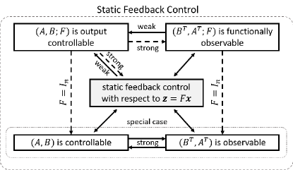
Figure 4: Relation between output controllability, functional observability, and static feedback system design for target control (with arbitrary pole placement). Solid arrows indicate that a given property implies another while dashed arrows indicate that a property implies another under certain conditions.

Following the proof of Theorem 3, if $(B^{\mathsf{T}},A^{\mathsf{T}};F)$ is functionally observable, then $\bm{z}=F\bm{x}=F_{c}\bm{x}_{c}$ is only a function of the controllable states. Thus, for any given number $\alpha\in\mathbb{C}$, there exist a static feedback matrix $K$ such that the solution of the closed-loop system $\dot{\bm{x}}=(A-BK+\alpha I_{n})\bm{x}$ satisfies $\lim_{t\rightarrow\infty}(F\bm{x}(t)-\bar{\bm{z}})=0$ for any initial condition $\bm{x}(0)$, where $\bar{\bm{z}}\in\mathbb{R}^{n}$ is a steady state. Therefore, Theorem 3 establishes a necessary and sufficient condition for the stabilization problem of a target vector $\bm{z}(t)$ via static feedback control, which can be achieved by placing the eigenpairs $(\lambda_{i},\bm{v}_{ij})\in\Sigma$ on the left half of the complex plane. This is evident in the following special case.

Remark 9.

If $A$ is diagonalizable, then $\bm{z}(t)=F\bm{x}(t)=F\sum_{i}^{n}\bm{v}_{i1}^{\mathsf{T}}\bm{x}(0)\bm{v}^{\prime}_{i1}e^{\lambda_{i}t}$, where $\bm{v}_{i1}$ and $\bm{v}^{\prime}_{i1}$ are respectively the left and right eigenvectors associated with the eigenvalue $\lambda_{i}$ of $A$. This implies that the dynamical response of $\bm{z}(t)$ depends only on eigenvalues $\lambda_{i}$ that satisfy $F\bm{v}^{\prime}_{i1}\neq 0$. Following Theorem 3, all eigenpairs $(\lambda_{i},\bm{v}_{i1})$ that satisfy $F\bm{v}^{\prime}_{i1}\neq 0$ belong to $\Sigma$ and can be arbitrarily placed.

Our results elucidate that output controllability is too weak of a condition for the design of static feedback systems for target control, therefore being restricted to more permissive control laws such as the Gramian-based law (5). Theorem 3 shows that, to achieve target control via static feedback with arbitrary pole placement, a stronger notion than output controllability is required: the dual system must be functionally observable and, therefore, strong duality must hold (Corollary 1). Fig. 4 summarizes the relationship between these properties.

Remark 10.

Theorem 3 generalizes the well-known relation between static feedback system design (with arbitrary poles) and full-state controllability [35, Theorem 8.M3]. By definition, for $F=I_{n}$, $\Sigma$ contains all the eigenpairs of $A$. Therefore, following Theorem 3, all eigenvalues of $A$ can be arbitrarily placed if and only if $(B^{\mathsf{T}},A^{\mathsf{T}})$ is full-state observable. Since strong duality always holds for $F=I_{n}$ (Remark 4), this condition holds if and only if $(A,B)$ is full-state controllable.

Remark 11.

A geometric condition for the existence of a solution to the partial pole placement problem is also presented in Theorem 4.4 of Ref. [36]. For a triple $(A,B;F)$, this theorem states that every eigenpair in $\Sigma$ can be arbitrarily placed in the closed-loop system $(A-BK)$ if and only if $\mathcal{X}_{\Sigma}\subseteq\langle A|\imaginary(B)\rangle+\mathcal{V}^{*}$, where $\mathcal{X}_{\Sigma}=\{\bm{v}_{ij}\in\mathbb{R}^{n}:(\lambda_{i},\bm{v}_{ij})\in\Sigma\}$ is the modal subspace of $A$ that influences the dynamics of $\bm{z}(t)$ and $\mathcal{V}^{*}$ is the supremal element among all the $(A,B)$-invariant subspaces contained in $\operatorname{Ker}(F)$. Despite the strong geometric interpretation of this theorem, testing the condition above for $\mathcal{X}_{\Sigma}$ requires determining $\mathcal{V}^{*}$, which can be involved and computationally demanding for large-scale systems. In contrast, Theorem 3 provides an equivalent, but much simpler, existence condition that is solely based on the algebraic rank condition (6) for the functional observability of the dual system $(B^{\mathsf{T}},A^{\mathsf{T}};F)$.

4.1 Output feedback control and separation principle

Thus far, we have considered two paired systems that are each either output controllable or functionally observable. Now, we integrate the two properties in a single system (1)–(2) that is simultaneously output controllable and functionally observable, albeit with respect to different functionals $F$. We investigate a particular class of problems in control theory known as target control via (observer-based) output feedback. These problems can be formulated as the target control problem discussed above under the restriction of output feedback rather than full-state feedback. In other words, we assume that the full-state vector $\bm{x}$ is not directly measurable and, therefore, the feedback signal $\bm{u}=-K\bm{x}$ must be estimated from the output signal $\bm{y}$ using an observer.

The output feedback problem can be solved even if $\bm{x}$ is not entirely reconstructible (i.e., $(C,A)$ is unobservable), as long as the feedback signal $\bm{u}=-K\bm{x}$ can be estimated from $\bm{y}$ (i.e., $(C,A;-K)$ is functionally observable). To show this, we recall some results related to functional observability and functional observers. Consider the functional observer [10]

$$\dot{\bm{w}} =N\bm{w}+J\bm{y}+H\bm{u},$$ (28)

$$\hat{\bm{z}} =D\bm{w}+E\bm{y},$$ (29)

where $\hat{\bm{z}}\in\mathbb{R}^{r}$ is the output of a functional observer, $\bm{w}\in\mathbb{R}^{n_{0}}$ is an auxiliary state vector, and $(N,J,H,D,E)$ are design matrices of consistent dimensions. The functional observer (28)–(29) is stable if the functional observer’s output $\hat{\bm{z}}$ of the functional observer asymptotically converges to the target vector $\bm{z}=F\bm{x}$ (i.e., $\lim_{t\rightarrow\infty}(\bm{z}(t)-\hat{\bm{z}}(t))=0$). The necessary and sufficient conditions for this convergence are [10, Thm. 1]:

$$N\,\,\text{is Hurwitz},$$ (30)

$$NT+JC-TA=0,$$ (31)

$$H-TB=0,$$ (32)

$$F-DT-EC=0.$$ (33)

Moreover, there exist design matrices $(N,J,H,D,E)$ that satisfies the above conditions if and only if the triple $(C,A;F)$ is functionally observable [13, 32].

The next theorem establishes a separation principle between the design of a target feedback controller and of a functional observer. This allows the output feedback target control problem to be solved if the systems $(B^{\mathsf{T}},A^{\mathsf{T}};F)$ and $(C,A;-K)$ are functionally observable. The functional observability of $(B^{\mathsf{T}},A^{\mathsf{T}};F)$ guarantees the existence of a matrix $K$ that arbitrarily places the poles of the closed-loop system (23) associated with the target subspace (3), whereas the functional observability of $(C,A;-K)$ guarantees that the designed input $\bm{u}=-K\bm{x}$ can be directly estimated from the output signal $\bm{y}$ via a functional observer (28)–(29).

Theorem 4 (Separation principle).

Consider a system (1)–(2) coupled with the functional observer-based feedback controller

$$\dot{\bm{w}}=N\bm{w}+J\bm{y},$$ (34)

$${\bm{u}}=D\bm{w}+E\bm{y}.$$ (35)

Let Eq. (3) define the target vector sought to be controlled. The closed-loop system has a characteristic polynomial

$$p(\lambda)=\operatorname{det}(\lambda I_{n}-A+BK)\operatorname{det}(\lambda I_{n_{0}}-N).$$ (36)

There exists a feedback matrix $K$ and functional observer matrices $(N,J,D,E)$ such that the roots $p(\lambda_{i})=0$ can be arbitrarily placed for every eigenpair $(\lambda_{i},\bm{v}_{ij})\in\Sigma$ and every eigenvalue $\lambda_{i}$ of matrix $N$ if the triples $(B^{\mathsf{T}},A^{\mathsf{T}};F)$ and $(C,A;-K)$ are both functionally observable.

Proof.

Substituting (34) and (35) into (1) leads to the augmented dynamical system

$$\begin{bmatrix}\dot{\bm{x}}\\ \dot{\bm{w}}\end{bmatrix}=\begin{bmatrix}A+BEC&BD\\ JC&N\end{bmatrix}\begin{bmatrix}{\bm{x}}\\ {\bm{w}}\end{bmatrix}.$$ (37)

Let $-K\bm{x}$ be the functional sought to be estimated by the functional observer (34)–(35). Given that $(C,A;-K)$ is functionally observable by assumption, there exist matrices $(N,J,D,E)$ such that conditions (31)–(33) are satisfied for $F\leftarrow-K$. The functional observer is stable (i.e., $\lim_{t\rightarrow\infty}({\bm{u}}(t)+K\bm{x}(t))=0$) if and only if $\lim_{t\rightarrow\infty}(\bm{w}(t)-T\bm{x}(t))=0$ for some $T$. Applying the coordinate transformation $\bm{e}=\bm{w}-T\bm{x}$ to (37) yields the closed-loop system

$$\begin{bmatrix}\dot{\bm{x}}\\ \dot{\bm{e}}\end{bmatrix}=\begin{bmatrix}A-BK&BD\\ 0&N\end{bmatrix}\begin{bmatrix}{\bm{x}}\\ {\bm{e}}\end{bmatrix},$$ (38)

where the equalities (31)–(33) were applied. Given that the matrix in Eq. (38) is block triangular, the eigenvalues of the closed-loop system and the functional observer’s estimation error depend exclusively on $(A-BK)$ and $N$, leading to the characteristic polynomial (36).

Let system (38) be decomposed as (25) via a similarity transformation $\bar{\bm{x}}=P\bm{x}$, yielding $\operatorname{det}(\lambda I_{n}-A+BK)=\operatorname{det}(\lambda I_{m}-A_{c}+B_{c}K_{c})\operatorname{det}(\lambda I_{n-m}-A_{u})$. Since $(A_{c},B_{c})$ is controllable, then there exists some matrix $KP^{\mathsf{T}}=[K_{c}\,\,K_{u}]$ such that all roots of the polynomial $\operatorname{det}(\lambda I_{m}-A_{c}+B_{c}K_{c})$ can be arbitrarily placed. From Theorem 3, since $(B^{\mathsf{T}},A^{\mathsf{T}};F)$ is functionally observable, it follows that all eigenpairs $(\lambda_{i},\bm{v}_{ij})\in\Sigma$, where $\lambda_{i}$ is also an eigenvalue of $A_{c}$, can be arbitrarily placed via some matrix $K$. ∎

Owing to the separation principle, the closed-loop system directly inherits the eigenvalues from the feedback system and the functional observer. Consequently, previous existence conditions and algorithms developed specifically for the design of target/partial controllers [29] and functional observers [13, 44, 45, 46] can be employed independently.

Remark 12.

Theorem 4 is a generalization of the classical separation principle between full-state controllers and observers [35, Section 8.8]. To see this, recall that full-state control ($F=I_{n}$) implies that $\Sigma$ is the set of all eigenpairs of $A$. Likewise, full-state observers are a special case of functional observers where $\bm{w}\in\mathbb{R}^{n}$ and $\lim_{t\rightarrow\infty}\hat{\bm{z}}(t)=I_{n}\bm{x}(t)$ is the asymptotic output of a functional observer (28)–(29). Thus, it follows from Theorem 4 that the closed-loop system has a characteristic polynomial (36) with arbitrarily placed roots for all eigenvalues $\lambda$ of $A$ and $N$ if $(B^{\mathsf{T}},A^{\mathsf{T}};I_{n})$ and $(C,A;I_{n})$ are functionally observable. The latter condition is equivalent to the observability of $(C,A)$, whereas the former condition is equivalent, by duality, to the controllability of $(A,B)$, resulting in the classical separation principle.

4.2 Example

Building on the previous example, consider the dynamical system (1) defined by the system matrix $A$ in (13), for $a_{22}=-1$ and $a_{33}=a_{44}=-3$, and an input matrix $B=[1\,\,0\,\,0\,\,0\,\,0]^{\mathsf{T}}$. Let the functional matrix (14) define the target vector (3) sought to be controlled. Fig. 5a provides a graph representation of the closed-loop system.

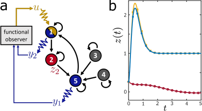
Figure 5: Target control via output feedback. (a) Graph representation of the closed-loop system for target control via output feedback. The input, output, and target variables are highlighted by yellow, blue and red nodes, respectively. Note that the input signal is the output of the functional observer. (b) State evolution of the target variable $\bm{z}(t)=x_{2}(t)$ in the open-loop system (red), closed-loop system via full-state feedback (blue), and closed-loop system via functional observer-based output feedback (yellow). The initial conditions were randomly drawn from an uniform distribution ($\bm{x}_{i}(0)\sim\mathcal{U}[0,1],\forall i$).

First, note that the system is uncontrollable ($\rank(\mathcal{C})=3<n$) and hence full-state control is not possible. However, since condition (6) is satisfied for the dual system $(B^{\mathsf{T}},A^{\mathsf{T}};F)$, the triple $(B^{\mathsf{T}},A^{\mathsf{T}};F)$ is functionally observable and, according to Theorem 3, the target control problem can be solved via static feedback. This is evident by applying the system decomposition (25) with $P=[\bm{e}_{1}\,\,\bm{e}_{2}\,\,\bm{e}_{4}\,\,\bm{e}_{5}\,\,\bm{e}_{3}]$, where $\bm{e}_{i}$ is a standard basis vector with 1 in the $j$th position and 0 elsewhere, and noting that $[F_{c}\,|\,F_{u}]=[0\,\,1\,\,0\,|\,0\,\,0]$ (with $F_{u}=0$, as expected from Theorem 3). The eigenvalues $\lambda=\{-2,-0.5\pm i0.866\}$ are associated with left eigenvectors $\bm{v}$ that satisfy $Q\bm{v}\neq 0$. Therefore, these eigenpairs belong to $\Sigma$ and can then be arbitrarily placed in the closed-loop system (23). On the other hand, the eigenpairs associated with $\lambda=-3$ (which cannot be arbitrarily placed) have eigenvectors with zero projection onto $\operatorname{row}(F)$. Consequently, these eigenpairs do not belong to $\Sigma$ and do not influence the dynamical response of $\bm{z}(t)$.

As an example, let the specifications for the target control problem be as follows. First, for the transient response of $\bm{z}(t)$, the desired position for the set of closed-loop poles in $\Sigma$ is $\{-4,-5,-6\}$. Second, for the steady-state response $\lim_{t\rightarrow\infty}\bm{z}(t)$, the desired setpoint is $\bm{z}^{*}=1$. These specifications can be simultaneously satisfied using an input signal $\bm{u}=\bm{r}-K\bm{x}$, where $K=[12\,\,-47\,\,0\,\,0\,\,59]$ and $\bm{r}=-120$. Fig. 5b shows simulations for the open-loop system as well as the target control system via static feedback. The reference signal $\bm{r}$ successfully sets the steady state of the target variable at the specified value $\bm{z}^{*}$, as intended. Moreover, the response of the target variable in the closed-loop system is substantially faster than in the open-loop system due to the leftward shift of the poles in the complex plane.

We now proceed to design the functional observer (34)–(35), solving the target control problem via output feedback. Let the output matrix be now extended as

$$C=\begin{bmatrix}0&0&0&0&1\\ 1&0&0&0&0\end{bmatrix}.$$ (39)

We can then verify that the system $(C,A;-K)$ is functionally observable via condition (6), which guarantees the existence of a stable functional observer capable of estimating the feedback signal $-K\bm{x}$ [13]. To determine the design matrices in (34)–(35), we follow the design procedure in [44, Section 3.6.1], yielding $N=-1$, $J=[0\,\,-47]$, $D=1$, $E=[-59\,\,-12]$, and $T=[0\,\,47\,\,0\,\,0\,\,0]$, which satisfy the conditions (30)–(33). Note that, following the separation principle, the design and pole placement of the feedback system (for target control) and the functional observer (for output feedback) were carried out independently. Similarly to the full-state feedback case, Fig. 5b shows that the target control via (functional observer-based) output feedback stabilizes the system at the setpoint $\bm{z}^{*}$ with a short transient response. The small difference in performance between the closed-loop systems with output feedback and full-state feedback is attributed to the convergence time of the functional observer (for random initial conditions).

5 Conclusion

Our results establish a duality principle between the generalized notions of output controllability and functional observability—properties that were conceived independently [12, 13] for the control and estimation of lower-order functions of the state variables. In contrast with the special cases of full-state controllability and observability, the relation between these generalized properties is not always bidirectional (functional observability always implies the output controllability of the dual system, but the converse is not necessarily true). The duality is strong (bidirectional) only under the condition that the controllable and the uncontrollable sets are orthogonal following a projection onto the row space of $F$. Drawing from the strong duality principle, we show that the target control of a system via static feedback is possible if and only if its dual system is functionally observable. Consequently, as in the full-state feedback control and estimation case, the design of a static feedback system (for target control) and of a functional observer (for output feedback) are independent, generalizing the well-known separation principle between controllers and observers.

Beyond the theoretical significance of connecting two previously unrelated properties, the duality established here is expected to allow techniques developed for functional observability to be employed in the study of output controllability, and vice versa. As shown in a recent application of this duality to structured systems [39], the weak duality principle enables algorithms developed to optimally place sensors for target estimation in large-scale networks [17] to be used to optimally place actuators for target control in such networks [14, 15, 20]; likewise, the converse can also be pursued when strong duality holds. Based on similar arguments, we expect that methods developed for the design of functional observers can also be used to design target controllers, and vice versa. In particular, the open problem of designing target controllers via dynamic feedback could then be approached by mapping the solution from a dual problem of functional observer design, which has well-established scalable solutions [10, 13, 33, 17]. As an application, in the control of cluster synchronized states, one may leverage design methods for functional observers originally developed for the estimation of average cluster states [47, 48].

Finally, given that the duality and separation principles between controllability and observability have been extended to many other classes of dynamical systems, including stochastic [49, 50], nonlinear [51, 52], and differential-algebraic [53] systems, we anticipate that the existence of a duality principle between the generalized notions of output controllability [54] and functional observability [55] can also be established for a broader class of dynamical systems than those considered here.

References

- [1] R. E. Kalman, “On the general theory of control systems,” IFAC Proceedings Volumes, vol. 1, no. 1, pp. 491–512, 1960.
- [2] A. E. Motter, “Networkcontrology,” Chaos, vol. 25, p. 097621, 2015.
- [3] Y.-Y. Liu and A.-L. Barabási, “Control principles of complex systems,” Reviews of Modern Physics, vol. 88, p. 035006, 2016.
- [4] A. N. Montanari and L. A. Aguirre, “Observability of Network Systems: A Critical Review of Recent Results,” Journal of Control, Automation and Electrical Systems, vol. 31, no. 6, pp. 1348–1374, 2020.
- [5] T. Parmer and F. Radicchi, “Dynamical methods for target control of biological networks,” Royal Society Open Science, vol. 10, p. 230542, 2023.
- [6] F. Pasqualetti, S. Zampieri, and F. Bullo, “Controllability, Limitations and Algorithms for Complex Networks,” IEEE Transactions on Control of Network Systems, vol. 1, no. 1, pp. 40–52, 2013.
- [7] T. H. Summers, F. L. Cortesi, and J. Lygeros, “On Submodularity and Controllability in Complex Dynamical Networks,” IEEE Transactions on Control of Network Systems, vol. 3, no. 1, pp. 91–101, 2016.
- [8] G. Yan, G. Tsekenis, B. Barzel, J.-J. Slotine, Y.-Y. Liu, and A.-L. Barabási, “Spectrum of controlling and observing complex networks,” Nature Physics, vol. 11, no. 9, pp. 779–786, 2015.
- [9] G. Duan, A. Li, T. Meng, G. Zhang, and L. Wang, “Energy cost for controlling complex networks with linear dynamics,” Physical Review E, vol. 99, p. 052305, 2019.
- [10] M. Darouach, “Existence and Design of Functional Observers for Linear Systems,” IEEE Transactions on Automatic Control, vol. 45, no. 5, pp. 940–943, 2000.
- [11] V. I. Vorotnikov, “Partial stability and control: The state-of-the-art and development prospects,” Automation and Remote Control, vol. 66, pp. 3–59, 2005.
- [12] J. Bertram and P. Sarachik, “On optimal computer control,” IFAC Proceedings Volumes, vol. 1, no. 1, pp. 429–432, 1960.
- [13] T. L. Fernando, H. M. Trinh, and L. Jennings, “Functional Observability and the Design of Minimum Order Linear Functional Observers,” IEEE Transactions on Automatic Control, vol. 55, no. 5, pp. 1268–1273, 2010.
- [14] J. Gao, Y.-Y. Liu, R. M. D’Souza, and A.-L. Barabási, “Target control of complex networks,” Nature Communications, vol. 5, p. 5415, 2014.
- [15] H. J. van Waarde, M. K. Camlibel, and H. L. Trentelman, “A Distance-Based Approach to Strong Target Control of Dynamical Networks,” IEEE Transactions on Automatic Control, vol. 62, no. 12, pp. 6266–6277, 2017.
- [16] G. Casadei, C. Canudas-de-Wit, and S. Zampieri, “Model Reduction Based Approximation of the Output Controllability Gramian in Large-Scale Networks,” IEEE Transactions on Control of Network Systems, vol. 7, no. 4, pp. 1778–1788, 2020.
- [17] A. N. Montanari, C. Duan, L. A. Aguirre, and A. E. Motter, “Functional observability and target state estimation in large-scale networks,” Proceedings of the National Academy of Sciences of the U.S.A., vol. 119, p. e2113750119, 2022.
- [18] Y. Zhang, R. Cheng, and Y. Xia, “Observability Blocking for Functional Privacy of Linear Dynamic Networks,” arXiv:2304.07928, 2023.
- [19] F. L. Iudice, F. Sorrentino, and F. Garofalo, “On Node Controllability and Observability in Complex Dynamical Networks,” IEEE Control Systems Letters, vol. 3, no. 4, pp. 847–852, 2019.
- [20] E. Czeizler, K. C. Wu, C. Gratie, K. Kanhaiya, and I. Petre, “Structural Target Controllability of Linear Networks,” IEEE/ACM Transactions on Computational Biology and Bioinformatics, vol. 15, no. 4, pp. 1217–1228, 2018.
- [21] C. Commault, J. van der Woude, and P. Frasca, “Functional target controllability of networks: Structural properties and efficient algorithms,” IEEE Transactions on Network Science and Engineering, vol. 7, no. 3, pp. 1521–1530, 2019.
- [22] Y.-Y. Liu, J.-J. Slotine, and A.-L. Barabási, “Controllability of complex networks,” Nature, vol. 473, pp. 167–73, 2011.
- [23] M. Siami and A. Jadbabaie, “A separation theorem for joint sensor and actuator scheduling with guaranteed performance bounds,” Automatica, vol. 119, 2020.
- [24] M. Balinski and A. W. Tucker, “Duality theory of linear programs: A constructive approach with applications,” SIAM Review, vol. 11, no. 3, pp. 347–377, 1969.
- [25] E. Y. Hamedani and N. S. Aybat, “A Decentralized Primal-Dual Method for Constrained Minimization of a Strongly Convex Function,” IEEE Transactions on Automatic Control, vol. 67, no. 11, pp. 5682–5697, 2022.
- [26] M. Lazar and J. Lohéac, “Output controllability in a long-time horizon,” Automatica, vol. 113, p. 108762, 2020.
- [27] K. Ogata, Modern Control Engineering, 5th ed. Prentice Hall, 2010.
- [28] A. S. Morse, “Output controllability and system synthesis,” SIAM Journal on Control, vol. 9, no. 2, pp. 143–148, 1971.
- [29] V. I. Vorotnikov, Partial stability and control. Birkhauser, 1998.
- [30] J. Li, X. Chen, S. Pequito, G. J. Pappas, and V. M. Preciado, “On the structural target controllability of undirected networks,” IEEE Transactions on Automatic Control, vol. 66, no. 10, pp. 4836–4843, 2020.
- [31] B. M. Shali, H. J. Van Waarde, M. K. Camlibel, and H. L. Trentelman, “Properties of Pattern Matrices with Applications to Structured Systems,” IEEE Control Systems Letters, vol. 6, pp. 109–114, 2022.
- [32] L. S. Jennings, T. L. Fernando, and H. M. Trinh, “Existence conditions for functional observability from an eigenspace perspective,” IEEE Transactions on Automatic Control, vol. 56, no. 12, pp. 2957–2961, 2011.
- [33] F. Rotella and I. Zambettakis, “A note on functional observability,” IEEE Transactions on Automatic Control, vol. 61, no. 10, pp. 3197–3202, 2016.
- [34] G. E. Dullerud and F. Paganini, A Course in Robust Control Theory: A Convex Approach. Springer Science & Business Media, 2013, vol. 36.
- [35] C.-T. Chen, Linear System Theory and Design, 3rd ed. Oxford University Press, 1999.
- [36] W. M. Wonham, Linear Multivariable Control: A Geometric Approach. Springer-Verlag, 1979.
- [37] G. Basile and G. Marro, Controlled and Conditioned Invariants in Linear Systems Theory. Prentice Hall, 1991.
- [38] ——, “Controlled and conditioned invariant subspaces in linear system theory,” Journal of Optimization Theory and Applications, vol. 3, pp. 306–315, 1969.
- [39] A. N. Montanari, C. Duan, and A. E. Motter, “Target controllability and target observability of structured network systems,” IEEE Control Systems Letters, vol. 7, pp. 3060–3065, 2023.
- [40] J. Sun and A. E. Motter, “Controllability transition and nonlocality in network control,” Physical Review Letters, vol. 110, p. 208701, 2013.
- [41] G. Yan, J. Ren, Y.-C. Lai, C.-H. Lai, and B. Li, “Controlling complex networks: How much energy is needed?” Physical Review Letters, vol. 108, no. 21, p. 218703, 2012.
- [42] A.-L. Barabási and R. Albert, “Emergence of Scaling in Random Networks,” Science, vol. 286, no. 5439, pp. 509–512, 1999.
- [43] D. J. Watts and S. H. Strogatz, “Collective dynamics of ‘small-world’ networks,” Nature, vol. 393, pp. 440–442, 1998.
- [44] H. Trinh and T. Fernando, Functional Observers for Dynamical Systems. Springer Berlin Heidelberg, 2012.
- [45] F. Rotella and I. Zambettakis, “A direct design procedure for linear state functional observers,” Automatica, vol. 70, pp. 211–216, 2016.
- [46] H. Habibi, T. Fernando, and M. Darouach, “On the functional observer design with sampled measurement,” IEEE Transactions on Automatic Control, vol. 68, no. 9, pp. 5759–5766, 2023.
- [47] M. U. B. Niazi, C. Canudas-de-Wit, and A. Y. Kibangou, “Average state estimation in large-scale clustered network systems,” IEEE Transactions on Control of Network Systems, vol. 7, no. 4, pp. 1736–1745, 2020.
- [48] M. U. B. Niazi, X. Cheng, C. Canudas-de-Wit, and J. M. Scherpen, “Clustering-based average state observer design for large-scale network systems,” Automatica, vol. 151, p. 110914, 2023.
- [49] H. F. Chen, “On stochastic observability and controllability,” Automatica, vol. 16, no. 2, pp. 179–190, 1980.
- [50] T. T. Georgiou and A. Lindquist, “The Separation Principle in Stochastic Control, Redux,” IEEE Transactions on Automatic Control, vol. 58, no. 10, pp. 2481–2494, 2013.
- [51] R. Hermann and A. J. Krener, “Nonlinear Controllability and Observability,” IEEE Transactions on Automatic Control, vol. 22, no. 5, pp. 728–740, 1977.
- [52] S. Kilicaslan and S. P. Banks, “A separation theorem for nonlinear systems,” Automatica, vol. 45, no. 4, pp. 928–935, 2009.
- [53] S. L. Campbell, N. K. Nichols, and W. J. Terrell, “Duality, observability, and controllability for linear time-varying descriptor systems,” Circuits Systems and Signal Processing, vol. 10, no. 4, pp. 455–470, 1991.
- [54] L. Tie, “Output-controllability and output-near-controllability of driftless discrete-time bilinear systems,” SIAM Journal on Control and Optimization, vol. 58, pp. 2114–2142, 2020.
- [55] A. N. Montanari, L. Freitas, D. Proverbio, and J. Gonçalves, “Functional observability and subspace reconstruction in nonlinear systems,” Physical Review Research, vol. 4, p. 043195, 12 2022.