Competing magnetic states on the surface of multilayer ABC-stacked graphene
Abstract
We study interaction-mediated magnetism on the surface of ABC-multilayer graphene driven by its zero-energy topological flat bands. Using the random-phase approximation we treat onsite Hubbard repulsion and find multiple competing magnetic states, due to both intra- and inter-valley scattering, with the latter causing an enlarged magnetic unit cell. At half-filling and when the Hubbard repulsion is weak, we observe two different ferromagnetic orders. Once the Hubbard repulsion becomes more realistic, new ferrimagnetic orders arise with distinct incommensurate intra- or inter-valley scattering vectors depending on interaction strength and doping, leading to a multitude of competing magnetic states.
Graphene has for a long time attracted attention due to its extraordinary electronic and structural properties Geim and Novoselov (2007); Castro Neto et al. (2009); Novoselov et al. (2004). While ideal graphene does not exhibit magnetic properties, various derivatives of graphene do Fernández-Rossier and Palacios (2007); Son et al. (2006); Yazyev (2010); Sharpe et al. (2019a), e.g. in the presence of a sublattice imbalance Esquinazi et al. (2003); Palacios et al. (2008); Magda et al. (2014); Lemonik et al. (2012) or due to Landau levels McCann and Fal’ko (2006); Nomura and MacDonald (2006); Goerbig (2011); Young et al. (2014, 2014) or interlayer twists Bistritzer and MacDonald ; Sharpe et al. (2019a); Chen et al. (2020); Klebl et al. (2021); Gonzalez-Arraga et al. (2017a); Xu et al. (2018); Liu et al. (2019). In particular, modifications generating flat bands with a high density of states (DOS) close to the Fermi energy are prone to not only magnetism but generally correlated insulators and even superconductivity Cao et al. (2018a); Lu et al. (2019); Xie et al. (2019); Po et al. (2018); Li et al. (2010); Sharpe et al. (2019b); Choi et al. (2019); Cao et al. (2018b); Jiang et al. (2019); Andrei and MacDonald (2020); Löthman and Black-Schaffer (2017). The flat band dispersion quells the kinetic energy and thus even moderately weak electron-electron interaction generates various electronic orders.
In monolayer graphene, the large Fermi velocity generated by the linear -dispersion prevents electronic ordering. Bilayer AB-stacked (Bernal) and trilayer ABC-stacked (rhombohedral) graphene instead host quadratic and cubic band dispersions, respectively, resulting in possibilities for electronic instabilities, with bilayer Velasco Jr et al. (2012); Geisenhof et al. (2021); Gonzalez-Arraga et al. (2017b); Zhou et al. (2022); Pangburn et al. (2022); Crépieux et al. (2023); Pantaleón et al. (2023); Marchenko et al. (2018), trilayer Lee et al. (2014); Yankowitz et al. (2014); Pangburn et al. (2022); Crépieux et al. (2022); Zhou et al. (2021), and also tetralayer graphene Myhro et al. (2018); Kerelsky et al. (2021) having been found to exhibit magnetic, as well as superconducting ordering, but so far only with the application of electric and/or magnetic fields Avetisyan et al. (2009); Min et al. (2007); Gava et al. (2009); Koshino (2010); Lui et al. (2011); Zhang et al. (2010). Further stacking of layers in an ABC-sequence produces a locally flat band dispersion on the surfaces of the stack, protected by topology Heikkilä et al. (2011); Heikkilä and Volovik (2011); McClure (1969); Henck et al. (2018). These flat surface states have already been shown to host versatile Fermi surface properties Min and MacDonald (2008); Zhang et al. (2010); Koshino (2010); Yuan et al. (2011); Bao et al. (2011); Jung and MacDonald (2013a); Lui et al. (2011); Gao et al. (2020); Kaladzhyan et al. (2021) leading to magnetism Shi et al. (2020); Hagymási et al. (2022); Pamuk et al. (2017a); Henni et al. (2016); Lee et al. (2022); Otani et al. (2010a); Xiao et al. (2011a); Cuong et al. (2012a); Pamuk et al. (2017b); Han et al. (2023) and theory proposals also exist for superconductivity, without any need for external fields Löthman and Black-Schaffer (2017); Awoga et al. (2023); Heikkilä et al. (2011); Kopnin et al. (2011); Kopnin (2011).
Most of the theoretical understanding of ABC-stacked multilayer graphene (ABC-MLG) is based on work, including ab-initio calculations, studying only the primitive (in-plane) unit cell and then finding surface ferrimagnetism; opposite magnetic moments on the two sublattices with one moment substantially suppressed Otani et al. (2010b); Xu et al. (2012); Olsen et al. (2013); Pamuk et al. (2017c); Xiao et al. (2011b); Cuong et al. (2012b); Awoga et al. (2023). Experiments have at the same time reported domain formation Shi et al. (2020), recently interpreted as competition between a ferrimagnetic state and a suggested quantum paramagnetic state, but also with an indication of longer-range magnetic ordering Hagymási et al. (2022). In this work we study the formation of magnetic ordering on the surface of ABC-MLG, in particular, taking into account all possible magnetic ordering patterns.
We use the -matrix formalism to isolate the ABC-MLG surface Green’s function and then incorporate electronic interactions in the form of Hubbard on-site repulsion within the matrix random-phase approximation (RPA). We find strong ordering tendencies for both intra- and inter-valley scattering, generating single and extended unit cell magnetic patterns, respectively. At half-filling, we find putative ferromagnetic (FM) ordering centered on one sublattice only and mediated by the non-interacting flat bands, but which is quickly suppressed for small interactions . At more realistic -values we find opposite but unequal moments on the two sublattices, rendering ferrimagnetic (FiM) orders and at incommensurate scattering vectors. The inter-valley ordering requires lower for ordering, while the intra-valley ordering is close to the (commensurate) ferrimagnetic order reported in earlier work Otani et al. (2010b); Xu et al. (2012); Olsen et al. (2013); Pamuk et al. (2017c); Xiao et al. (2011b); Cuong et al. (2012b); Awoga et al. (2023); Hagymási et al. (2022). Adding finite doping, intra-valley ordering instead requires the lowest , with a smaller incommensurability and a substantially shorter spin-spin relaxation time. Our work establishes a fierce competition between different magnetic orders, as well as the importance of incommensurability.
Model and method.— To model ABC-MLG we consider a tight-binding model of the bulk in the basis , where () denotes sublattice A(B) in layer Kaladzhyan et al. (2021):
| (1) |
where , , , with , and is enumerating the orbitals (sites). Here () denotes the intra(inter)-layer hopping between (), while a finite inter-layer hopping between is responsible for trigonal warping, splitting the graphene Dirac cone into three satellite Dirac cones causing a triangular Fermi surface Jung and MacDonald (2013b). By using we capture bulk ABC-stacked graphite (quasi-2D ABC-trilayer graphene). We set eV, eV, intralayer nearest neighbor distance Å, and interlayer nearest neighbor distance while using both to model unwarped and warped ABC-MLG, and vary the chemical potential through Kaladzhyan et al. (2021).
As we are interested in the ABC-MLG surface, we introduce a virtual wall of impurities , separating the bulk system Eq. (1) into two semi-infinite pieces along the -direction. Following the -matrix formalism, we compute the surface Green’s function from the bulk Green’s function obtained from , using Pinon et al. (2020); Kaladzhyan et al. (2021) with and the Matsubara frequency. Finally, the Green’s function on the surfaces , i.e. adjacent to the impurity plane, is given by partial Fourier transform of in the -direction, using the notation 111We compute the Matsubara summations using the effective Ozaki’s summation ozakiContinuedFractionRepresentation2007). We perform the analytic continuation (). We verify that the surface spectral function , reproduces the surface flat bands following earlier results Kaladzhyan et al. (2021).
To include electron interactions we consider on-site intra-orbital Hubbard repulsion where is the occupation number for site , orbital , and spin . We track the influence of interactions on both charge and magnetic fluctuations by employing the RPA to extract the relevant susceptibilities. Magnetic phenomena are governed by the spin susceptibility matrix given by Scalapino et al. ; Graser et al. ; Kemper et al.
| (2) |
Here the non-interacting, or bare, susceptibility matrix of size is constructed from the surface non-interacting Green’s function with elements
| (3) |
where denotes the number of sublattice sites, indexed as , while accounts for the scattering momentum, is the number of momentum modes, and is the inverse temperature. The spin interaction matrix takes the simple form Graser et al. (2009). To extract magnetically ordered states we use the density-density correlation functions, namely the homogeneous spin susceptibility Mahan (2000); Bruus and Flensberg (2004), also experimentally tractable Kreisel et al. (2022),
| (4) |
In particular, we compute the real [imaginary] parts of the homogeneous contributions for both the bare susceptibility, [], and the RPA susceptibility []. In a similar treatment for the charge susceptibility, we find that it always remains small compared to the spin susceptibility. We thus conclude that charge fluctuations are not important in ABC-MLG.
A divergent RPA susceptibility signals the formation of an ordered state, for magnetism expressed by the (generalized) Stoner criterion with Sakakibara et al. (2012). We thus obtain the critical Hubbard interaction strength for magnetic ordering from the maximum positive eigenvalue . We perform this analysis over the full first Brillouin zone (BZ) to capture longer-range magnetic ordering patterns beyond single-unit cell ordering, including incommensurate ordering. The eigenvector , associated with the eigenvalue once the Stoner criterion is satisfied, encodes the spatial structure of the magnetic order Fong et al. (2000); Gao et al. (2010); Boehnke (2015); Christensen et al. (2016); Fischer et al. (2022). Furthermore, a resonance structure in the dynamic profile of at specific in the ordered regime, i.e. for , can be assigned as the spin gap of the underlying order Fong et al. (2000); Gao et al. (2010); Christensen et al. (2016).
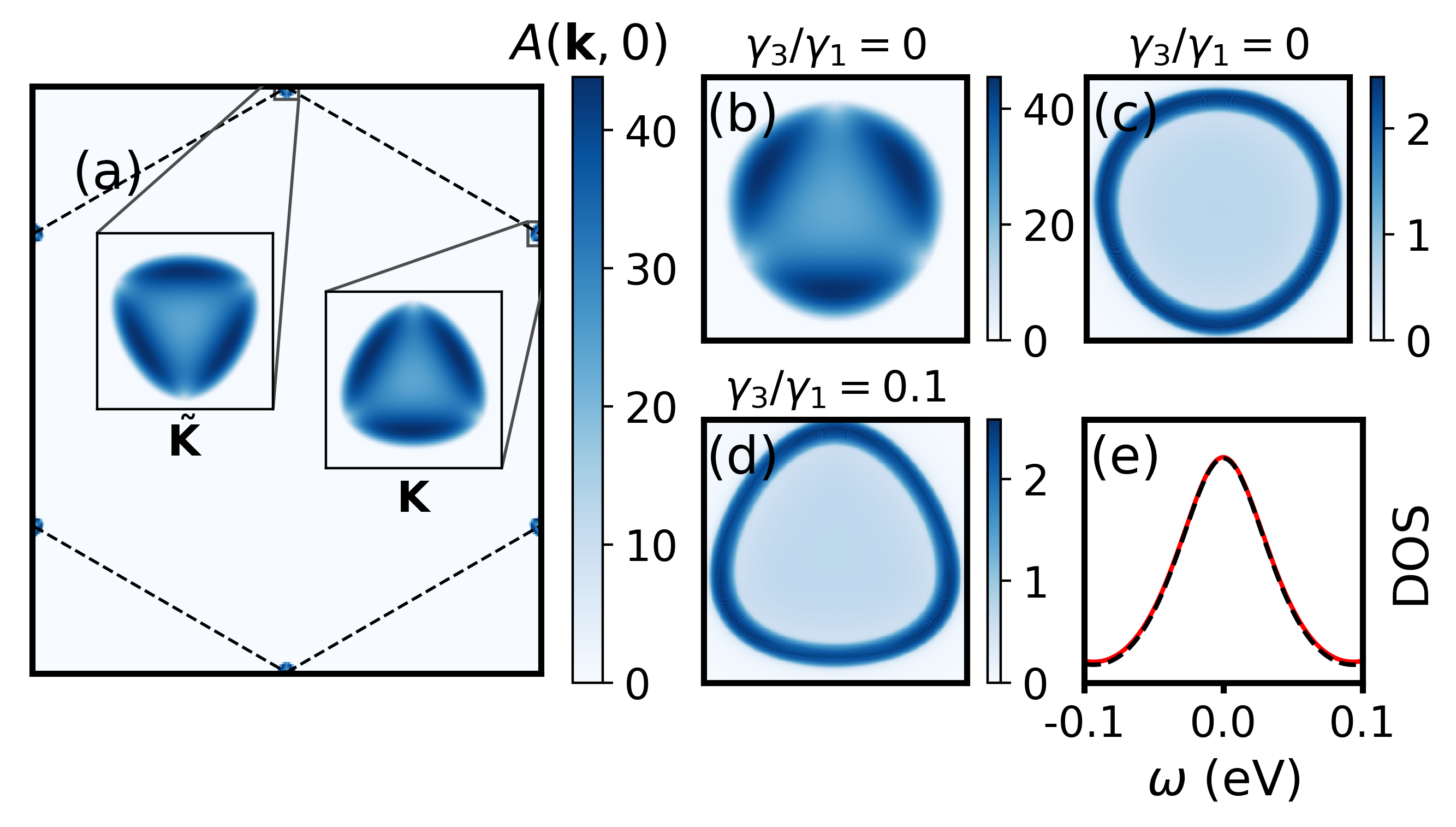
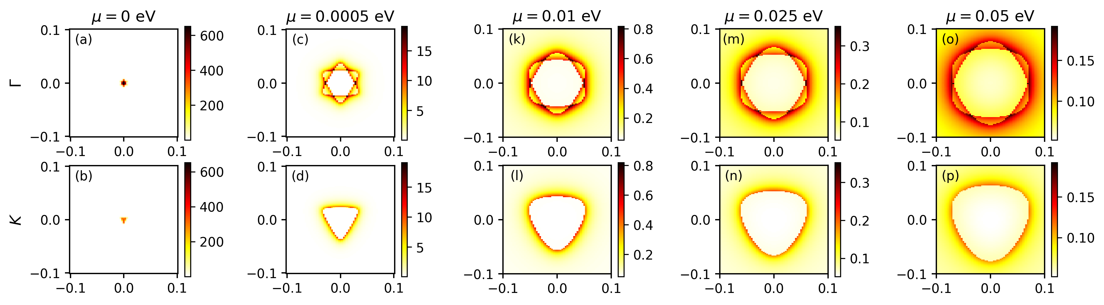
Flat bands and nesting.— We start by analyzing the non-interacting surface states of ABC-MLG. Fig. 1(a) shows how the surface spectral function acquires substantial weight, signaling a flat band area, around the points in a tripartite manner due to the three satellite Dirac points Jung and MacDonald (2013b). It is the trigonal warping that gives the triangular shape, while if set to zero a circular shape is instead achieved, see Fig. 1(b). Moving away from half-filling, the surface spectral function takes the shape of an annular ring, see Figs. 1(c,d), now instead capturing the bulk (dispersive) Dirac cones. The resulting DOS is plotted in Fig. 1(e) as a function of doping, showing no notable effect of warping. This demonstrates the extent and shape of the zero-energy surface flat bands.
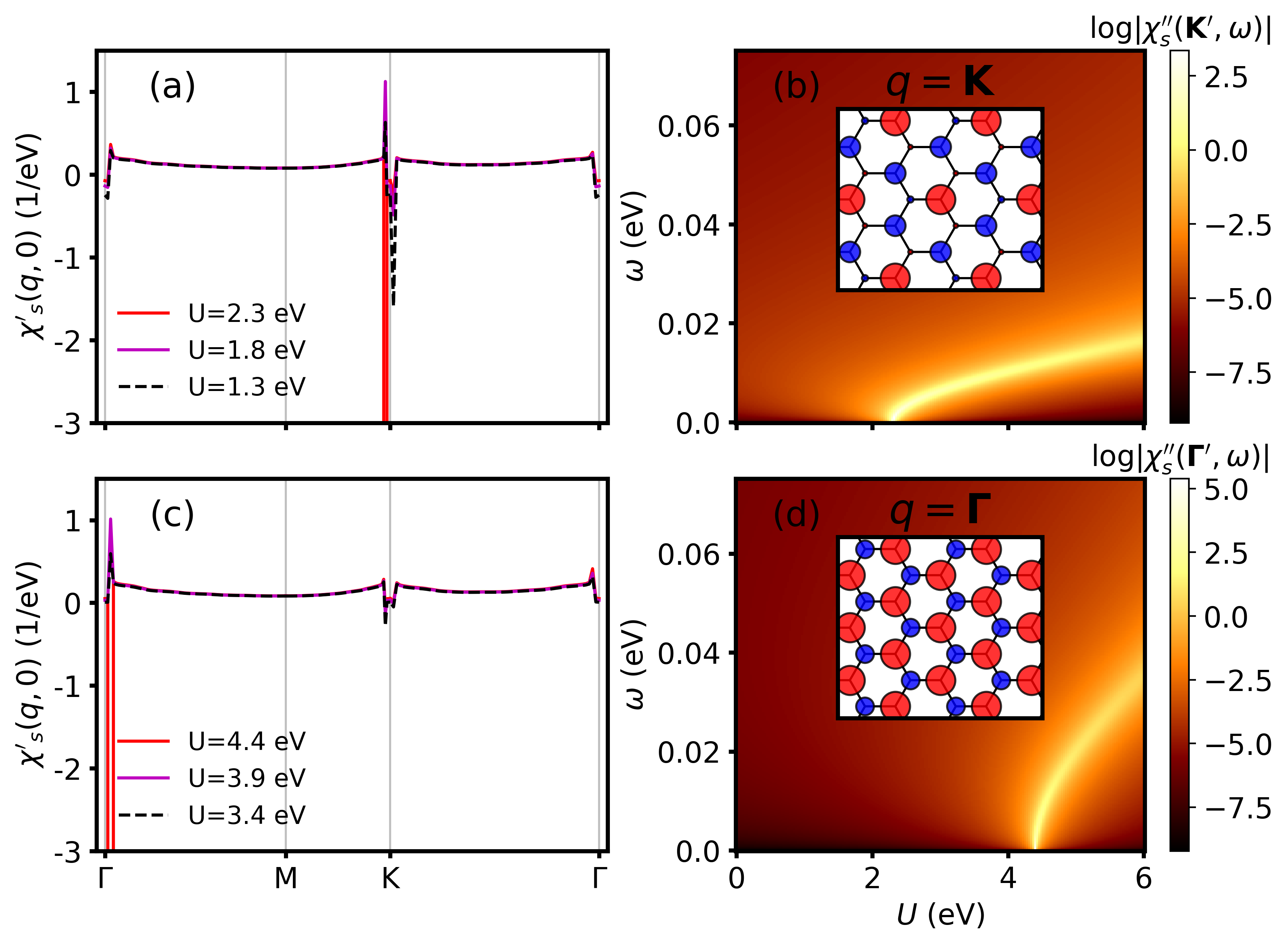
The existence of two Fermi surfaces, around and , leads to both intra- and inter-valley scattering with scattering, or nesting, vectors , respectively. This suggests that more than one type of magnetic order, with different ’s, may be present. Before investigating magnetic ordering driven by finite interactions, we analyze the effect of nesting on the bare spin susceptibility. In Fig. 2(a) we plot the real static non-interacting susceptibility at and note large values in small regions and , with divergences at the commensurate nesting vectors . The finite region are due to the finite extent of the surface flat bands. Away from half-filling, instead shows only finite peaks in the same regions, see Fig. 2(b). Thus divergences in the bare susceptibility are only present due to the zero-energy flat bands and limited to half-filling. This follows directly from the standard representation of the bare homogeneous susceptibility , with the Fermi-Dirac distribution, where the energy denominator vanishes for the flat bands. We further find no notable dependence on the trigonal warping .

With a divergent bare spin susceptibility, even an infinitesimal small interaction triggers magnetic ordering at half-filling according to the generalized Stoner criteria. Analyzing the resulting eigenvectors at and , we find magnetic moments only on the top surface’s orbital. For the -ordering the magnetic moment is also modulated in real space, acquiring zero net magnetization. Due to this magnetic structure, we refer to both of these states as sublattice ferromagnetic (sFM) order and note that they originate from commensurate nesting vectors. To gain more understanding of the sFM orders, we examine the imaginary part of the dynamic bare spin susceptibility at the divergent scattering vectors in Figs. 2(b,d) as a function of small . We find a large (negative) peak starting from and ending at with eV for and eV for . This indicates the existence of a finite spin gap protecting the sFM orders, but only for . Although the -sFM state has zero magnetization and absence of time-reversal symmetry, the characteristic two-resonance structure of chiral magnons in altermagnets Maier and Okamoto (2023); Šmejkal et al. (2023) is not seen, so this order is unlikely to emerge. For a more in-depth discussion on the sFM orders and their susceptibilities, see Supplementary Material (SM) sup .
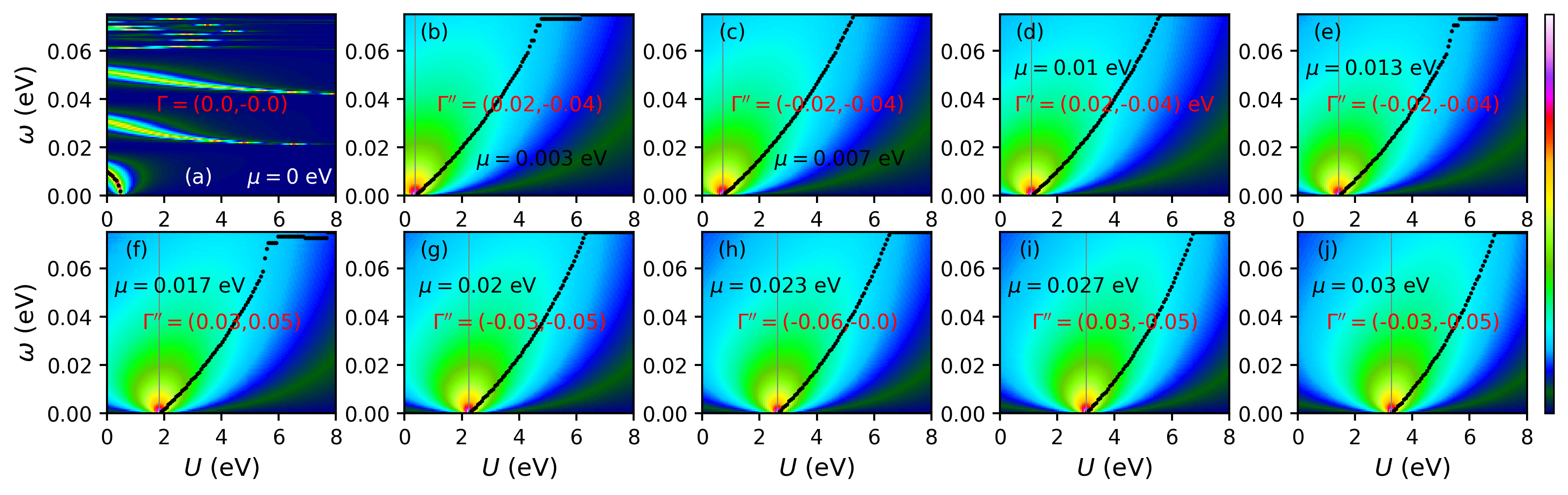
FiM order with interactions.— With and estimations of the on-site repulsion in graphene and graphite instead giving Wehling et al. (2011); Tancogne-Dejean and Rubio (2020); Bursill et al. (1998); Vergés et al. (2010), we do not expect the sFM solutions to likely exist in ABC-MLG. We thus continue analyzing the spin susceptibility for more realistic , here first at half-filling. We find that as increases beyond , the static spin susceptibility becomes substantially suppressed at both . We instead observe new divergences appearing for inter-valley scattering at with eV and for intra-valley scattering at for eV, see Figs. 3(a,c). Both divergences appear at incommensurate scattering vectors, linked to the finite extent of the surface flat band and thus different from the non-interacting commensurate sFM states. We can qualitatively understand this shift in scattering vectors by noting that a finite interaction shifts the quasiparticle energies with a self-energy Berk and Schrieffer (1966), such that the momentum dependence of may be different from that of . We further note that the peak in changes from positive to negative values as soon as the Stoner criterion is satisfied at . The negatively valued divergency is necessary due to the previous magnetic transitions at found in the previous section, see SM sup .
In terms of the resulting magnetic moments for the state, we find that the dominant contribution to comes from the top surface orbital and now also with the orbital carrying an unequal finite magnetic moment but with opposite sign, as illustrated in the Fig. 3(d) inset (incommensurability not visible). A similar analysis of the state results in the pattern in the Fig. 3(b) inset, again with dominant contribution from a orbital, but now with a extended spatial repetition, due to the inter-valley scattering, see SM sup . We note that the sum of all spin densities within the enlarged unit cell is exactly zero in the commensurate case. Given the incommensurability, the system acquires a small but non-zero magnetization. Therefore, we refer to the and states as incommensurate ferrimagnetic (FiM) orders.
Moreover, we consider the dynamic profile of in Fig. 3(b,d), now at the incommensurate wave vectors hosting the divergent (real) spin susceptibility 222The change to incommensurate wave vectors means the peaks in Fig. 2(b,c) at small for commensurate vectors are not visible in Fig. 3(b,d).. We find a large positive peak originating at and and rising to larger frequencies with increasing . This signals the existence of finite spin gaps Bruus and Flensberg (2004); Kreisel et al. (2022), confirming the formation of first a -FiM state at from inter-valley scattering and then a -FiM ordered state at from intra-valley scattering. With the spin susceptibility at becoming substantially suppressed at , see Fig. 3(c), we infer that the -FiM order likely directly set in at with little competition from the -FiM order, see SM sup . We further find that varies slightly with trigonal warping, producing slightly different ’s, but not changing the overall behavior. Taken together, these results point to a close competition between the -FiM and -FiM states at half-filling, such that any spatial dependence of will likely create spontaneous domains of different FiM states.
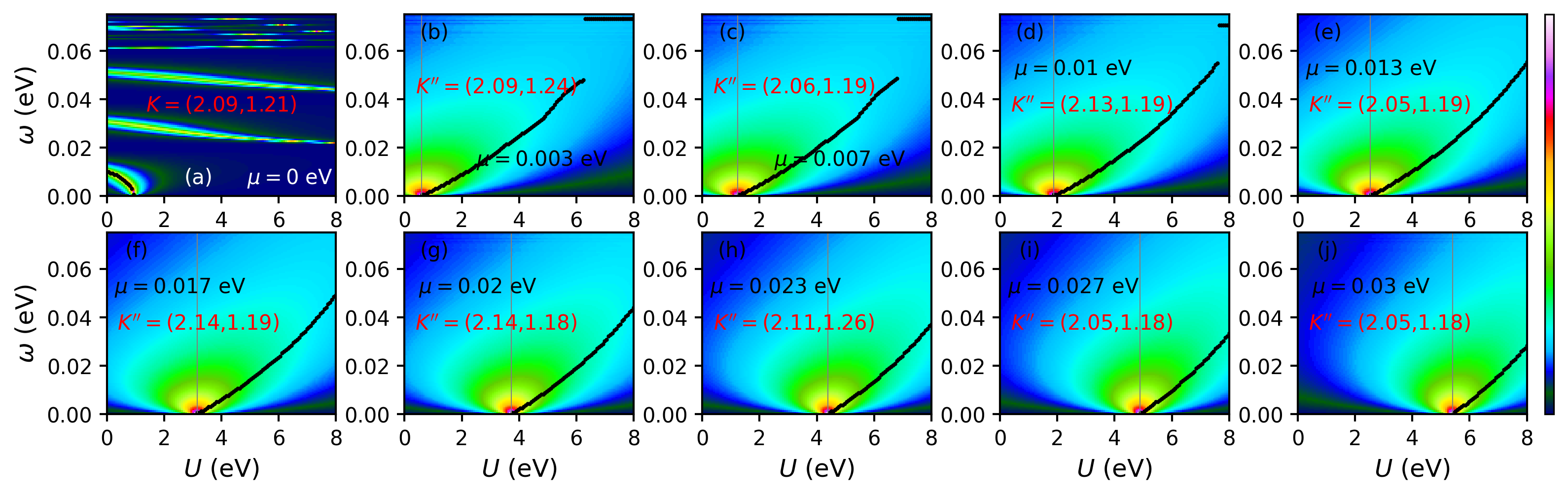
Finite doping.— Finally, we vary the doping away from half-filling, modeling spontaneous charge inhomogeneity Hagymási et al. (2022) or an applied gate voltage Shi et al. (2020); Hagymási et al. (2022). To probe the doping dependence, we extract the minimum critical Hubbard parameter at zero temperature satisfying the Stoner criterion for any nesting vector in discs centered at to capture all previously explored divergences and beyond. In Fig. 4 we plot the result as a function of doping and find increasing for both intra-valley (red) and inter-valley scattering (blue), with higher for the latter. At eV the results coincide with Fig. 2 with its commensurate orders already at . With increasing doping, we find a roughly linear increase in , while at the same time, the ordering vectors move away from . The resulting scattering vectors are labeled and , and the order as - and -FiM orders as they show large similarities with the FiM orders, see SM sup .
We plot the deviation and similar for in the inset of Fig. 4. There is a sharp jump in directly when acquires finite value, followed by a slow increase for increasing . We find that fully tracks the position of the finite amplitude peaks in the bare susceptibility, see Fig. 2(c) for a fixed . Thus magnetic ordering at finite doping is fully determined by the bare susceptibility with the interaction just enhancing its peaks into divergences at . This is notably different from the half-filled case where the interaction also shifts the ordering vectors to incommensurate vectors, compare Figs. 2(a) and 3(a,c).
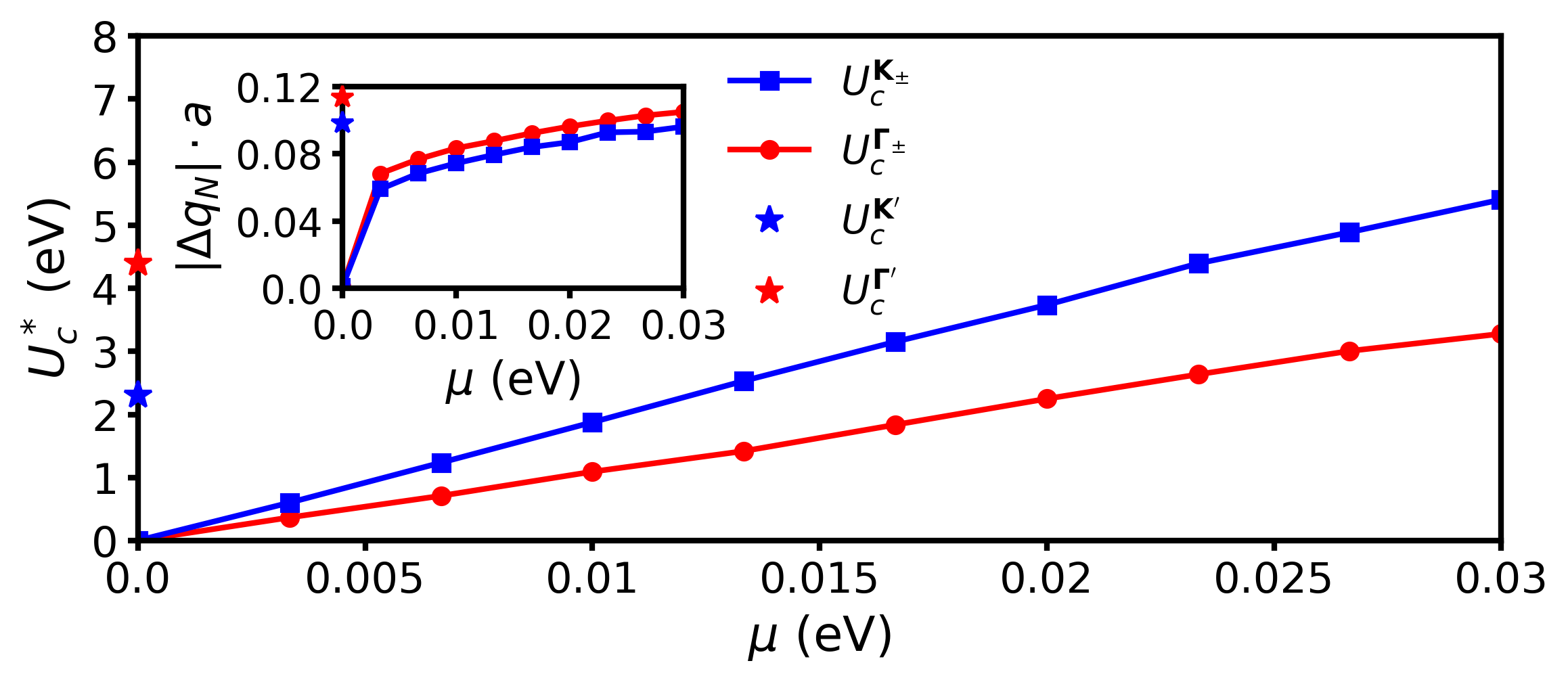
To highlight further differences to the half-filling results in Fig. 3, we mark with stars in Fig. 4. As seen, at half-filling inter-valley FiM order commands the lowest , while at any finite doping where intra-valley scattering has the lowest . Also, the incommensurability is always largest at half-filling, which seems to provide an upper limit for at finite doping. We also find a notably different overall behavior of the spin susceptibility. At half-filling a clear spin gap is present at , protecting the commensurate sFM orders until its closure at , while at , a new spin gap develops protecting the FiM orders as shown in Figs. 2(b,d) and 3(b,d). Instead, at finite doping no spin gap, or order, exists for any . Moreover, when ordering is established at , we find no sharp peaks at finite frequencies in . The dynamic susceptibility displays signatures of a markedly short spin-spin relaxation time Barra and Hassan (2005); Yalçın (2013), flattening the peaks in and also making continuous at non-zero frequencies. We attribute the shortened relaxation time to more substantial overlap with the dispersive surface states at finite doping Maier and Okamoto (2023), generating damping. Interestingly, the bulk metallic states do not generate any strong damping, as obvious from orders at half-filling. Still tracing a spin gap from the (flattened) peaks in , we find that they never disappear with increasing , once developed at . For more information, see SM sup . Based on the different s and their trends, scattering vectors, and different relaxation times, we conclude that the states at finite doping are notably different from those at half-filling.
Concluding remarks.— Our work reveals how the surface flat band in ABC-multilayer graphene leads to a plethora of magnetic states. At half-filling, commensurate sFM orders with either intra- and inter-valley nesting vectors in the non-interacting limit. At any realistic interaction strength, incommensurate FiM orders instead develop for both intra- and inter-valley scattering. Away from half-filling, interactions result in another set of incommensurate FiM orders with different nesting vectors and a notably short spin-spin relaxation time. This demonstrates remarkably rich possibilities for different magnetic ordering on the surface ABC-MLG, both competing intra- and inter-valley scattering states, and also different states with varying interaction and doping.
Connecting to recent experimental findings, all our states fall within the layer antiferromagnet (LAF) phase recently found in pentalayer ABC-stacked graphene Han et al. (2023); Zhang et al. (2011) and establish the rich and varying surface magnetic structures of this phase. Other findings, reporting a (commensurate) gapped antiferromagnetic order at half-filling with an enlarged magnetic unit cell away from it, together with a quantum paramagnetic phase Hagymási et al. (2022), are similar to our - and )-FiM states. Importantly, we find that both incommensurability and magnetic pattern vary intricately with interaction strength and doping. Such close competition between multiple states may also enhance the importance of quantum fluctuations.
L.B. thanks G. B. Martins for insights on the RPA method and P. Holmvall for providing his code implementation of the Matsubara summations. We also thank X. Feng, D. Chakraborty, R. Arouca, P. M. Oppeneer, and P. Thundström for fruitful discussions. We acknowledge financial support from the Knut and Alice Wallenberg Foundation, through the Wallenberg Academy Fellows program and project grant KAW 2019.0068.
References
- Geim and Novoselov (2007) A. K. Geim and K. S. Novoselov, Nature materials 6, 183 (2007).
- Castro Neto et al. (2009) A. H. Castro Neto, F. Guinea, N. M. R. Peres, K. S. Novoselov, and A. K. Geim, Rev. Mod. Phys. 81, 109 (2009).
- Novoselov et al. (2004) K. S. Novoselov, A. K. Geim, S. V. Morozov, D.-e. Jiang, Y. Zhang, S. V. Dubonos, I. V. Grigorieva, and A. A. Firsov, science 306, 666 (2004).
- Fernández-Rossier and Palacios (2007) J. Fernández-Rossier and J. J. Palacios, Phys. Rev. Lett. 99, 177204 (2007).
- Son et al. (2006) Y.-W. Son, M. L. Cohen, and S. G. Louie, Phys. Rev. Lett. 97, 216803 (2006).
- Yazyev (2010) O. V. Yazyev, Reports on Progress in Physics 73, 056501 (2010).
- Sharpe et al. (2019a) A. L. Sharpe, E. J. Fox, A. W. Barnard, J. Finney, K. Watanabe, T. Taniguchi, M. Kastner, and D. Goldhaber-Gordon, Science 365, 605 (2019a).
- Esquinazi et al. (2003) P. Esquinazi, D. Spemann, R. Höhne, A. Setzer, K.-H. Han, and T. Butz, Phys. Rev. Lett. 91, 227201 (2003).
- Palacios et al. (2008) J. J. Palacios, J. Fernández-Rossier, and L. Brey, Phys. Rev. B 77, 195428 (2008).
- Magda et al. (2014) G. Z. Magda, X. Jin, I. Hagymási, P. Vancsó, Z. Osváth, P. Nemes-Incze, C. Hwang, L. P. Biro, and L. Tapasztó, Nature 514, 608 (2014).
- Lemonik et al. (2012) Y. Lemonik, I. Aleiner, and V. I. Fal’ko, Phys. Rev. B 85, 245451 (2012).
- McCann and Fal’ko (2006) E. McCann and V. I. Fal’ko, Phys. Rev. Lett. 96, 086805 (2006).
- Nomura and MacDonald (2006) K. Nomura and A. H. MacDonald, Phys. Rev. Lett. 96, 256602 (2006).
- Goerbig (2011) M. O. Goerbig, Rev. Mod. Phys. 83, 1193 (2011).
- Young et al. (2014) A. Young, J. Sanchez-Yamagishi, B. Hunt, S. Choi, K. Watanabe, T. Taniguchi, R. Ashoori, and P. Jarillo-Herrero, Nature 505, 528 (2014).
- (16) R. Bistritzer and A. H. MacDonald, 108, 12233, 21730173 .
- Chen et al. (2020) G. Chen, A. L. Sharpe, E. J. Fox, Y.-H. Zhang, S. Wang, L. Jiang, B. Lyu, H. Li, K. Watanabe, T. Taniguchi, et al., Nature 579, 56 (2020).
- Klebl et al. (2021) L. Klebl, Z. A. H. Goodwin, A. A. Mostofi, D. M. Kennes, and J. Lischner, Phys. Rev. B 103, 195127 (2021).
- Gonzalez-Arraga et al. (2017a) L. A. Gonzalez-Arraga, J. L. Lado, F. Guinea, and P. San-Jose, Phys. Rev. Lett. 119, 107201 (2017a).
- Xu et al. (2018) X. Y. Xu, K. T. Law, and P. A. Lee, Phys. Rev. B 98, 121406 (2018).
- Liu et al. (2019) J. Liu, Z. Ma, J. Gao, and X. Dai, Phys. Rev. X 9, 031021 (2019).
- Cao et al. (2018a) Y. Cao, V. Fatemi, S. Fang, K. Watanabe, T. Taniguchi, E. Kaxiras, and P. Jarillo-Herrero, Nature 556, 43 (2018a).
- Lu et al. (2019) X. Lu, P. Stepanov, W. Yang, M. Xie, M. A. Aamir, I. Das, C. Urgell, K. Watanabe, T. Taniguchi, G. Zhang, A. Bachtold, A. H. MacDonald, and D. K. Efetov, Nature 574, 653 (2019).
- Xie et al. (2019) Y. Xie, B. Lian, B. Jäck, X. Liu, C.-L. Chiu, K. Watanabe, T. Taniguchi, B. A. Bernevig, and A. Yazdani, Nature 572, 101 (2019).
- Po et al. (2018) H. C. Po, L. Zou, A. Vishwanath, and T. Senthil, Physical Review X 8, 031089 (2018).
- Li et al. (2010) G. Li, A. Luican, J. M. B. Lopes dos Santos, A. H. Castro Neto, A. Reina, J. Kong, and E. Y. Andrei, Nature Physics 6, 109 (2010).
- Sharpe et al. (2019b) A. L. Sharpe, E. J. Fox, A. W. Barnard, J. Finney, K. Watanabe, T. Taniguchi, M. A. Kastner, and D. Goldhaber-Gordon, Science 365, 605 (2019b).
- Choi et al. (2019) Y. Choi, J. Kemmer, Y. Peng, A. Thomson, H. Arora, R. Polski, Y. Zhang, H. Ren, J. Alicea, G. Refael, F. von Oppen, K. Watanabe, T. Taniguchi, and S. Nadj-Perge, Nature Physics 15, 1174 (2019).
- Cao et al. (2018b) Y. Cao, V. Fatemi, A. Demir, S. Fang, S. L. Tomarken, J. Y. Luo, J. D. Sanchez-Yamagishi, K. Watanabe, T. Taniguchi, E. Kaxiras, R. C. Ashoori, and P. Jarillo-Herrero, Nature 556, 80 (2018b).
- Jiang et al. (2019) Y. Jiang, X. Lai, K. Watanabe, T. Taniguchi, K. Haule, J. Mao, and E. Y. Andrei, Nature 573, 91 (2019).
- Andrei and MacDonald (2020) E. Y. Andrei and A. H. MacDonald, Nature materials 19, 1265 (2020).
- Löthman and Black-Schaffer (2017) T. Löthman and A. M. Black-Schaffer, Phys. Rev. B 96, 064505 (2017).
- Velasco Jr et al. (2012) J. Velasco Jr, L. Jing, W. Bao, Y. Lee, P. Kratz, V. Aji, M. Bockrath, C. Lau, C. Varma, R. Stillwell, et al., Nat. Nanotechnol. 7, 156 (2012).
- Geisenhof et al. (2021) F. R. Geisenhof, F. Winterer, A. M. Seiler, J. Lenz, T. Xu, F. Zhang, and R. T. Weitz, Nature 598, 53 (2021).
- Gonzalez-Arraga et al. (2017b) L. A. Gonzalez-Arraga, J. L. Lado, F. Guinea, and P. San-Jose, Phys. Rev. Lett. 119, 107201 (2017b).
- Zhou et al. (2022) H. Zhou, L. Holleis, Y. Saito, L. Cohen, W. Huynh, C. L. Patterson, F. Yang, T. Taniguchi, K. Watanabe, and A. F. Young, Science 375, 774 (2022).
- Pangburn et al. (2022) E. Pangburn, L. Haurie, A. Crépieux, O. A. Awoga, A. M. Black-Schaffer, C. Pépin, and C. Bena, “Superconductivity in monolayer and few-layer graphene: I. Review of possible pairing symmetries and basic electronic properties,” (2022), arxiv:2211.05146 [cond-mat] .
- Crépieux et al. (2023) A. Crépieux, E. Pangburn, L. Haurie, O. A. Awoga, A. M. Black-Schaffer, N. Sedlmayr, C. Pépin, and C. Bena, Physical Review B 108, 134515 (2023).
- Pantaleón et al. (2023) P. A. Pantaleón, A. Jimeno-Pozo, H. Sainz-Cruz, V. T. Phong, T. Cea, and F. Guinea, Nature Reviews Physics 5, 304 (2023).
- Marchenko et al. (2018) D. Marchenko, D. Evtushinsky, E. Golias, A. Varykhalov, T. Seyller, and O. Rader, Science advances 4, eaau0059 (2018).
- Lee et al. (2014) Y. Lee, D. Tran, K. Myhro, J. Velasco, N. Gillgren, C. Lau, Y. Barlas, J. Poumirol, D. Smirnov, and F. Guinea, Nature communications 5, 5656 (2014).
- Yankowitz et al. (2014) M. Yankowitz, J. I.-J. Wang, A. G. Birdwell, Y.-A. Chen, K. Watanabe, T. Taniguchi, P. Jacquod, P. San-Jose, P. Jarillo-Herrero, and B. J. LeRoy, Nature materials 13, 786 (2014).
- Crépieux et al. (2022) A. Crépieux, E. Pangburn, L. Haurie, O. A. Awoga, A. M. Black-Schaffer, N. Sedlmayr, C. Pépin, and C. Bena, “Superconductivity in monolayer and few-layer graphene: II. Topological edge states and Chern numbers,” (2022), arxiv:2211.11778 [cond-mat] .
- Zhou et al. (2021) H. Zhou, T. Xie, T. Taniguchi, K. Watanabe, and A. F. Young, Nature 598, 434 (2021).
- Myhro et al. (2018) K. Myhro, S. Che, Y. Shi, Y. Lee, K. Thilahar, K. Bleich, D. Smirnov, and C. Lau, 2D Materials 5, 045013 (2018).
- Kerelsky et al. (2021) A. Kerelsky, C. Rubio-Verdú, L. Xian, D. M. Kennes, D. Halbertal, N. Finney, L. Song, S. Turkel, L. Wang, K. Watanabe, et al., Proceedings of the National Academy of Sciences 118, e2017366118 (2021).
- Avetisyan et al. (2009) A. A. Avetisyan, B. Partoens, and F. M. Peeters, Phys. Rev. B 80, 195401 (2009).
- Min et al. (2007) H. Min, B. Sahu, S. K. Banerjee, and A. H. MacDonald, Phys. Rev. B 75, 155115 (2007).
- Gava et al. (2009) P. Gava, M. Lazzeri, A. M. Saitta, and F. Mauri, Phys. Rev. B 79, 165431 (2009).
- Koshino (2010) M. Koshino, Phys. Rev. B 81, 125304 (2010).
- Lui et al. (2011) C. H. Lui, Z. Li, K. F. Mak, E. Cappelluti, and T. F. Heinz, Nature Physics 7, 944 (2011).
- Zhang et al. (2010) F. Zhang, B. Sahu, H. Min, and A. H. MacDonald, Phys. Rev. B 82, 035409 (2010).
- Heikkilä et al. (2011) T. T. Heikkilä, N. B. Kopnin, and G. E. Volovik, JETP Letters 94, 233 (2011).
- Heikkilä and Volovik (2011) T. T. Heikkilä and G. E. Volovik, JETP Letters 93, 59 (2011).
- McClure (1969) J. W. McClure, Carbon 7, 425 (1969).
- Henck et al. (2018) H. Henck, J. Avila, Z. Ben Aziza, D. Pierucci, J. Baima, B. Pamuk, J. Chaste, D. Utt, M. Bartos, K. Nogajewski, B. A. Piot, M. Orlita, M. Potemski, M. Calandra, M. C. Asensio, F. Mauri, C. Faugeras, and A. Ouerghi, Phys. Rev. B 97, 245421 (2018).
- Min and MacDonald (2008) H. Min and A. H. MacDonald, Phys. Rev. B 77, 155416 (2008).
- Yuan et al. (2011) S. Yuan, R. Roldán, and M. I. Katsnelson, Phys. Rev. B 84, 125455 (2011).
- Bao et al. (2011) W. Bao, L. Jing, J. Velasco Jr, Y. Lee, G. Liu, D. Tran, B. Standley, M. Aykol, S. Cronin, D. Smirnov, et al., Nature Physics 7, 948 (2011).
- Jung and MacDonald (2013a) J. Jung and A. H. MacDonald, Phys. Rev. B 88, 075408 (2013a).
- Gao et al. (2020) Z. Gao, S. Wang, J. Berry, Q. Zhang, J. Gebhardt, W. M. Parkin, J. Avila, H. Yi, C. Chen, S. Hurtado-Parra, et al., Nature communications 11, 546 (2020).
- Kaladzhyan et al. (2021) V. Kaladzhyan, S. Pinon, F. Joucken, Z. Ge, E. A. Quezada-Lopez, T. Taniguchi, K. Watanabe, J. Velasco, and C. Bena, Phys. Rev. B 104, 155418 (2021).
- Shi et al. (2020) Y. Shi, S. Xu, Y. Yang, S. Slizovskiy, S. V. Morozov, S.-K. Son, S. Ozdemir, C. Mullan, J. Barrier, J. Yin, et al., Nature 584, 210 (2020).
- Hagymási et al. (2022) I. Hagymási, M. S. Mohd Isa, Z. Tajkov, K. Márity, L. Oroszlány, J. Koltai, A. Alassaf, P. Kun, K. Kandrai, A. Pálinkás, et al., Science Advances 8, eabo6879 (2022).
- Pamuk et al. (2017a) B. Pamuk, J. Baima, F. Mauri, and M. Calandra, Physical Review B 95, 075422 (2017a).
- Henni et al. (2016) Y. Henni, H. P. Ojeda Collado, K. Nogajewski, M. R. Molas, G. Usaj, C. A. Balseiro, M. Orlita, M. Potemski, and C. Faugeras, Nano Letters 16, 3710 (2016).
- Lee et al. (2022) Y. Lee, S. Che, J. J. Velasco, X. Gao, Y. Shi, D. Tran, J. Baima, F. Mauri, M. Calandra, M. Bockrath, and C. N. Lau, Nano Letters 22, 5094 (2022).
- Otani et al. (2010a) M. Otani, M. Koshino, Y. Takagi, and S. Okada, Physical Review B 81, 161403 (2010a).
- Xiao et al. (2011a) R. Xiao, F. Tasnádi, K. Koepernik, J. W. F. Venderbos, M. Richter, and M. Taut, Physical Review B 84, 165404 (2011a).
- Cuong et al. (2012a) N. T. Cuong, M. Otani, and S. Okada, Surface Science 606, 253 (2012a).
- Pamuk et al. (2017b) B. Pamuk, J. Baima, F. Mauri, and M. Calandra, Physical Review B 95, 075422 (2017b).
- Han et al. (2023) T. Han, Z. Lu, G. Scuri, J. Sung, J. Wang, T. Han, K. Watanabe, T. Taniguchi, H. Park, and L. Ju, Nat. Nanotechnol. , https://doi.org/10.1038/s41565 (2023).
- Löthman and Black-Schaffer (2017) T. Löthman and A. M. Black-Schaffer, Physical Review B 96, 064505 (2017).
- Awoga et al. (2023) O. A. Awoga, T. Löthman, and A. M. Black-Schaffer, Physical Review B 108, 144504 (2023).
- Kopnin et al. (2011) N. B. Kopnin, T. T. Heikkilä, and G. E. Volovik, Physical Review B 83, 220503 (2011).
- Kopnin (2011) N. B. Kopnin, JETP Letters 94, 81 (2011).
- Otani et al. (2010b) M. Otani, M. Koshino, Y. Takagi, and S. Okada, Phys. Rev. B 81, 161403 (2010b).
- Xu et al. (2012) D.-H. Xu, J. Yuan, Z.-J. Yao, Y. Zhou, J.-H. Gao, and F.-C. Zhang, Phys. Rev. B 86, 201404 (2012).
- Olsen et al. (2013) R. Olsen, R. van Gelderen, and C. M. Smith, Phys. Rev. B 87, 115414 (2013).
- Pamuk et al. (2017c) B. Pamuk, J. Baima, F. Mauri, and M. Calandra, Phys. Rev. B 95, 075422 (2017c).
- Xiao et al. (2011b) R. Xiao, F. Tasnádi, K. Koepernik, J. W. F. Venderbos, M. Richter, and M. Taut, Phys. Rev. B 84, 165404 (2011b).
- Cuong et al. (2012b) N. T. Cuong, M. Otani, and S. Okada, Surface Science 606, 253 (2012b).
- Jung and MacDonald (2013b) J. Jung and A. H. MacDonald, Phys. Rev. B 88, 075408 (2013b).
- Pinon et al. (2020) S. Pinon, V. Kaladzhyan, and C. Bena, Phys. Rev. B 101, 115405 (2020).
- Note (1) We compute the Matsubara summations using the effective Ozaki’s summation ozakiContinuedFractionRepresentation2007). We perform the analytic continuation ().
- (86) D. J. Scalapino, E. Loh, and J. E. Hirsch, 34, 8190.
- (87) S. Graser, T. A. Maier, P. J. Hirschfeld, and D. J. Scalapino, 11, 025016.
- (88) A. F. Kemper, T. A. Maier, S. Graser, H.-P. Cheng, P. J. Hirschfeld, and D. J. Scalapino, 12, 073030.
- Graser et al. (2009) S. Graser, T. Maier, P. Hirschfeld, and D. Scalapino, New Journal of Physics 11, 025016 (2009).
- Mahan (2000) G. Mahan, “Many-body physics,” (2000).
- Bruus and Flensberg (2004) H. Bruus and K. Flensberg, Many-body quantum theory in condensed matter physics: an introduction (OUP Oxford, 2004).
- Kreisel et al. (2022) A. Kreisel, P. Hirschfeld, and B. M. Andersen, Frontiers in Physics , 241 (2022).
- Sakakibara et al. (2012) H. Sakakibara, H. Usui, K. Kuroki, R. Arita, and H. Aoki, Physical Review B 85, 064501 (2012).
- Fong et al. (2000) H. F. Fong, P. Bourges, Y. Sidis, L. P. Regnault, J. Bossy, A. Ivanov, D. L. Milius, I. A. Aksay, and B. Keimer, Phys. Rev. B 61, 14773 (2000).
- Gao et al. (2010) Y. Gao, T. Zhou, C. S. Ting, and W.-P. Su, Phys. Rev. B 82, 104520 (2010).
- Boehnke (2015) L. V. Boehnke, Susceptibilities in Materials with Multiple Strongly Correlated Orbitals, doctoralThesis, Staats- und Universitätsbibliothek Hamburg Carl von Ossietzky (2015).
- Christensen et al. (2016) M. H. Christensen, H. Jacobsen, T. A. Maier, and B. M. Andersen, Phys. Rev. Lett. 116, 167001 (2016).
- Fischer et al. (2022) A. Fischer, Z. A. Goodwin, A. A. Mostofi, J. Lischner, D. M. Kennes, and L. Klebl, npj Quantum Materials 7, 5 (2022).
- Maier and Okamoto (2023) T. A. Maier and S. Okamoto, Physical Review B 108, L100402 (2023).
- Šmejkal et al. (2023) L. Šmejkal, A. Marmodoro, K.-H. Ahn, R. González-Hernández, I. Turek, S. Mankovsky, H. Ebert, S. W. D’Souza, O. Šipr, J. Sinova, and T. Jungwirth, Physical Review Letters 131, 256703 (2023).
- (101) See Supplemental Material at XXXX-XXXX for discussions on dynamic spin susceptibility at half-filling as well as away from half-filling.
- Wehling et al. (2011) T. O. Wehling, E. Şaşıoğlu, C. Friedrich, A. I. Lichtenstein, M. I. Katsnelson, and S. Blügel, Physical Review Letters 106, 236805 (2011).
- Tancogne-Dejean and Rubio (2020) N. Tancogne-Dejean and A. Rubio, Physical Review B 102, 155117 (2020).
- Bursill et al. (1998) R. J. Bursill, C. Castleton, and W. Barford, Chemical Physics Letters 294, 305 (1998).
- Vergés et al. (2010) J. A. Vergés, E. SanFabián, G. Chiappe, and E. Louis, Physical Review B 81, 085120 (2010).
- Berk and Schrieffer (1966) N. F. Berk and J. R. Schrieffer, Phys. Rev. Lett. 17, 433 (1966).
- Note (2) The change to incommensurate wave vectors means the peaks in Fig. 2(b,c) at small for commensurate vectors are not visible in Fig. 3(b,d).
- Barra and Hassan (2005) A. L. Barra and A. K. Hassan, in Encyclopedia of Condensed Matter Physics, edited by F. Bassani, G. L. Liedl, and P. Wyder (Elsevier, Oxford, 2005) pp. 58–67.
- Yalçın (2013) O. Yalçın, in Ferromagnetic Resonance - Theory and Applications (IntechOpen, 2013).
- Zhang et al. (2011) F. Zhang, J. Jung, G. A. Fiete, Q. Niu, and A. H. MacDonald, Phys. Rev. Lett. 106, 156801 (2011).
Supplementary Material for “Competing magnetic states on the surface of multilayer ABC-stacked graphene”
Lauro B. Braz,1,2 Tanay Nag,2 and Annica Black-Schaffer,2
1Instituto de Física, Universidade de São Paulo, Rua do Matão 1371, São Paulo, São Paulo 05508-090, Brazil
2Department of Physics and Astronomy, Uppsala University, Box 516, 75120 Uppsala, Sweden
This Supplementary Material (SM) provides additional information supporting the results in the main text. In Section S1 we establish where in the Brillouin zone divergences in the spin-susceptibility appear. This warrants the choices of reciprocal coordinates in the figures in the main text. In Section S2 we provide additional data on the dynamic spin susceptibility in the non-interacting case and at low interactions at half-filling, supplementing the results in the section “Flat band and nesting effects” in the main text. In Section S3 we provide additional data on the dynamic spin susceptibility for realistic interaction strengths at half-filling, supplementing the results in the section “FiM order with interaction” in the main text. In Section S4 we provide additional data on the dynamic spin susceptibility at finite doping, supplementing the results in the section “Finite doping” in the main text. In Section S5 we demonstrate the additional analysis on the magnetic spin texture, supplementing the magnetic structures provided in section “FiM order with interactions” in the main text.
S1 Static susceptibility profile around the high-symmetry points
In the main text in Figs. 2 and 3 we investigate the behavior of the static susceptibility only along a high-symmetry BZ line. In this section, we provide additional data on the momentum profile of the static susceptibility motivating this choice for the half-filling case, while also demonstrating that it is not enough at arbitrary doping. We do so by examining the microscopic structure around the high-symmetry points and for the homogeneous spin susceptibility and the most dominating density-density element in at half-filling in Fig. S1 and away from half-filling in Fig. S2, respectively.
At half-filling we find that the static spin susceptibility diverges over a ring-like region around the and , see Fig. S1 upper (lower) panel for (). While the rings have a hexagonal (trigonal) distortion, they still respect the () rotational symmetry of the lattice, and the divergences are spread uniformly along the ring. Upon increasing , the ring expands but maintains the hexagonal (trigonal) symmetry. Overall, this analysis suggests the divergent nesting vectors move away from the commensurate nesting vectors and as only obtained for . Still, by keeping the hexagonal (trigonal) lattice symmetry with a uniform divergence along the perimeter, all scattering vectors with divergent susceptibility can be captured by only examining the high-symmetry line . This validates the choice of -values (along the -axis) in Figs. 2 and 3.
Next, we add a finite doping which causes the Fermi level to move away from the flat band region. We examine the static bare susceptibility as a function of finite doping in Fig. S2. At finite doping we find a star-like divergence instead of a ring divergence around point, see upper panel of Fig. S2, while it continues to form a triangular shape around , see lower panel of Fig. S2. Notably, the degree of divergence is not uniformly distributed over the star-like or triangle-like regions, rather there exist certain points yielding the strongest divergence. As a result, the equidistant nature of the divergent scattering momentum with respect to the high-symmetry points is no longer present. This means that the high-symmetry line through the BZ might not contain the strongest divergences. As a result, to capture the for the doped case, we need to go beyond the high-symmetry line such that we do not miss the correct order. We do this in Fig. 4 by extracting over the whole disc centered around and . We also note that the regions with star-like and triangle-like divergences expand with increasing doping, resulting in an outward shift in incommensurate nesting vectors with respect to the high-symmetry points, as also illustrated in the inset in Fig. 4.
As a naming convention, we refer to the incommensurate nesting vectors lying on the high-symmetry line as and in the case of half-filling. On the other hand, we adopt the and notation for the incommensurate nesting vectors in the case of finite doping that can lie both away from as well as on the high-symmetry line.
S2 Dynamic spin susceptibility analysis for zero and small at half-filling
In the main text we discuss the role of flat bands in forming magnetic order in the non-interacting system in the section “Flat band and nesting effects”. Here we provide additional data supporting those results. In particular, we present the full frequency behavior of the real part of the spin susceptibility (dashed lines) and the imaginary part of the spin susceptibility (solid lines) for zero and small values of at the commensurate nesting vectors (black), (red) in Fig. S3.
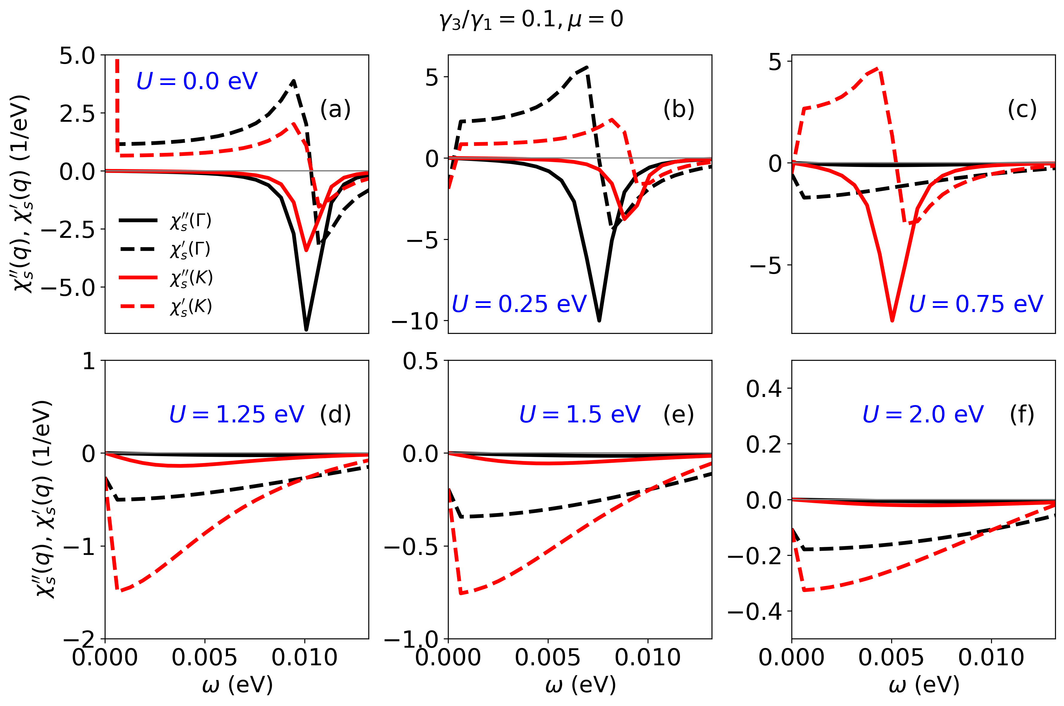
Before proceeding, we note that the susceptibility accounts for the probability of the scattering taking place with a transfer of momentum and energy . In general, the real part of the spin susceptibility estimates how much the system favors a particular magnetic order possibility, while the imaginary part encodes the loss in the system. We note that the gap along the frequency axis does not necessarily correspond to a spectral gap, rather it represents the energy barrier for opposite spin correlations. Therefore, the frequency where the susceptibility peaks can be considered to mark a spin gap associated with the magnetic order Bruus and Flensberg (2004).
Starting from in Fig. S3(a), we find a (negative) resonance peak at finite in the imaginary part of spin susceptibility for both and . Exactly at the same values of , the real parts exhibit a discontinuous jump. A closer inspection suggests that the real part changes its sign at a zero crossing where the imaginary part shows the resonance peak. This marks the existence of an ordered state with a finite spin gap for both intra- and inter-valley scattering already at . We also note that changes its sign from positive to negative as soon as an infinitesimal is considered. These features continue to exist for finite but small , except that the resonance peaks move steadily towards zero frequency when increases, see Fig. S3(b). Once crosses eV, the resonance peak as well as discontinuous jump for are not visible anymore and the ordering at is thus lost, see Fig. S3(c). The same occurs for inter-valley scattering at eV, see Fig. S3(d). Thus, beyond this ABC-MLG becomes magnetically disordered as far as the ordering vectors are concerned, see Fig. S3(e,f). We refer to the order at zero and small as the sFM orders in the main text, where Fig. 2 summarizes the main features in the susceptibility. In Sec. S5, we discuss the real-space pattern of the spin moments on the surface of the ABC-MLG.
Two additional points are worth commenting on. First, the critical values mark the termination of an ordered state. This is not determined by the Stoner criterion, which only marks the onset of ordering. Nonetheless, the clear vanishing of prominent features in the spin susceptibility, including the vanishing of a clear spin gap for makes it clear that the preceding order existing at lower values cannot exist anymore. Second, display a negatively valued peak. This is the opposite sign compared to the features marking the transitions at as shown below in Sec. S3 and Fig. S4. These different signs are required for the spin susceptibility to be continuous across the full range. Their existence also marks that the FiM orders occurring at must have had a predecessor ordering at lower values.
S3 Dynamic spin susceptibility analysis for finite at half-filling
In the main text, we show the existence of FiM order for realistic strengths of the Hubbard repulsion in the section “FiM orders with interactions” staying at half-filling. In this section of the SM, we provide additional data for the dynamic spin susceptibility with varying finite . In particular, the analysis is useful to further understand the magnetic phase transitions at eV and eV, established in Figs. 3 of the main text. We thus repeat Fig. S3 but now focus on larger values of and use the incommensurate nesting vectors . The results are presented in Fig. S4.
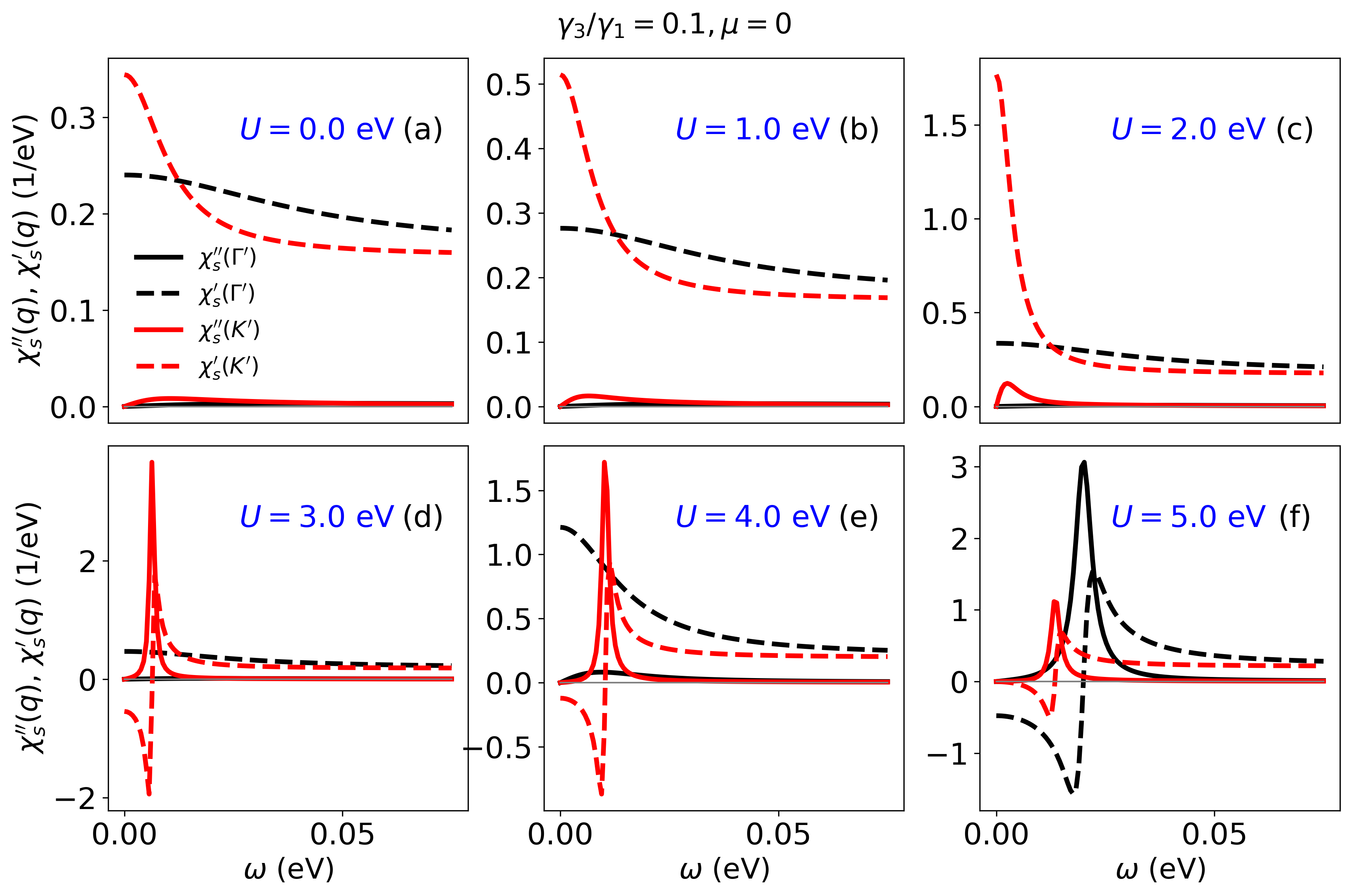
For comparison, we start with in Fig. S4(a) where we find and both decaying with from their values. On the other hand, both and start from zero at but then acquire a finite but small value very close to , before they again decay to zero with . We hence have no order at at , but the order only exists at the commensurate as seen in Fig. S3. With increasing , see Fig. S4(b,c), develops more and more of a peak at while simultaneously develops a peak at small and decreasing . Such a peak is referred to as a resonance phenomenon since the measure of such dynamic correlation changes with frequency. At the same time, no noticeable changes occur for for these values.
As soon as hits , forms a resonance peak at , which for is shifted to a finite value of , see Fig. S4(d). At the same time, changes its character from a single positive peak to a sign-changing divergence, or at least a discontinuous jump crossing the zero-line, appearing at at the transition and then moving to finite with increasing . The peaks/divergences in and are clearly appearing at the same (real part crosses zero when the imaginary part peaks) at and beyond . This exact matching of the real and imaginary spin susceptibility clearly marks the onset of magnetic ordering with ordering vector at , consistent with many earlier analyses of ordering within RPA calculations in other materials Christensen et al. (2016); Fong et al. (2000); Gao et al. (2010). We refer to this order in the main text as the -FiM state. The same evolution is also observed in Figs. S3(a,b,c) for in the sFM orders.
Moving on to larger values we find that the peak and discontinuous jumps in slowly decrease, see Fig. S4(e). Instead, we find that the same features as discussed above appear for an ordered magnetic state at , setting in at , see Fig. S4(f). As a consequence, for , -FiM order is formed. Due to the simultaneous suppression of the features in , we conclude that the -FiM may dominate at these larger values. This result supports the susceptibility results of Fig. 3 in the main text. In Sec. S5, we discuss the accompanied real-space pattern of the spin moments on the surface of the ABC-MLG.
S4 Dynamic spin susceptibility analysis with away from half-filling
In the main text, we analyze the case of finite doping away from half-filling in the section “Finite doping”. In this section of the SM, we provide additional data for the dynamic spin susceptibility. In Fig. S5 we redo the analysis of Figs. S3 and S4 for the representative doping level eV. This analysis is useful to understand the underlying data of Fig. 4 of the main text where we plot extracted as a function of . Note that we here are not restricted to a high-symmetry line in BZ when extracting the nesting vectors, but we identify the -values with divergent spin susceptibilities in a whole disc around . For notational consistency, we adopt , representation away from the half-filled cases as already mentioned in Sec. S1.
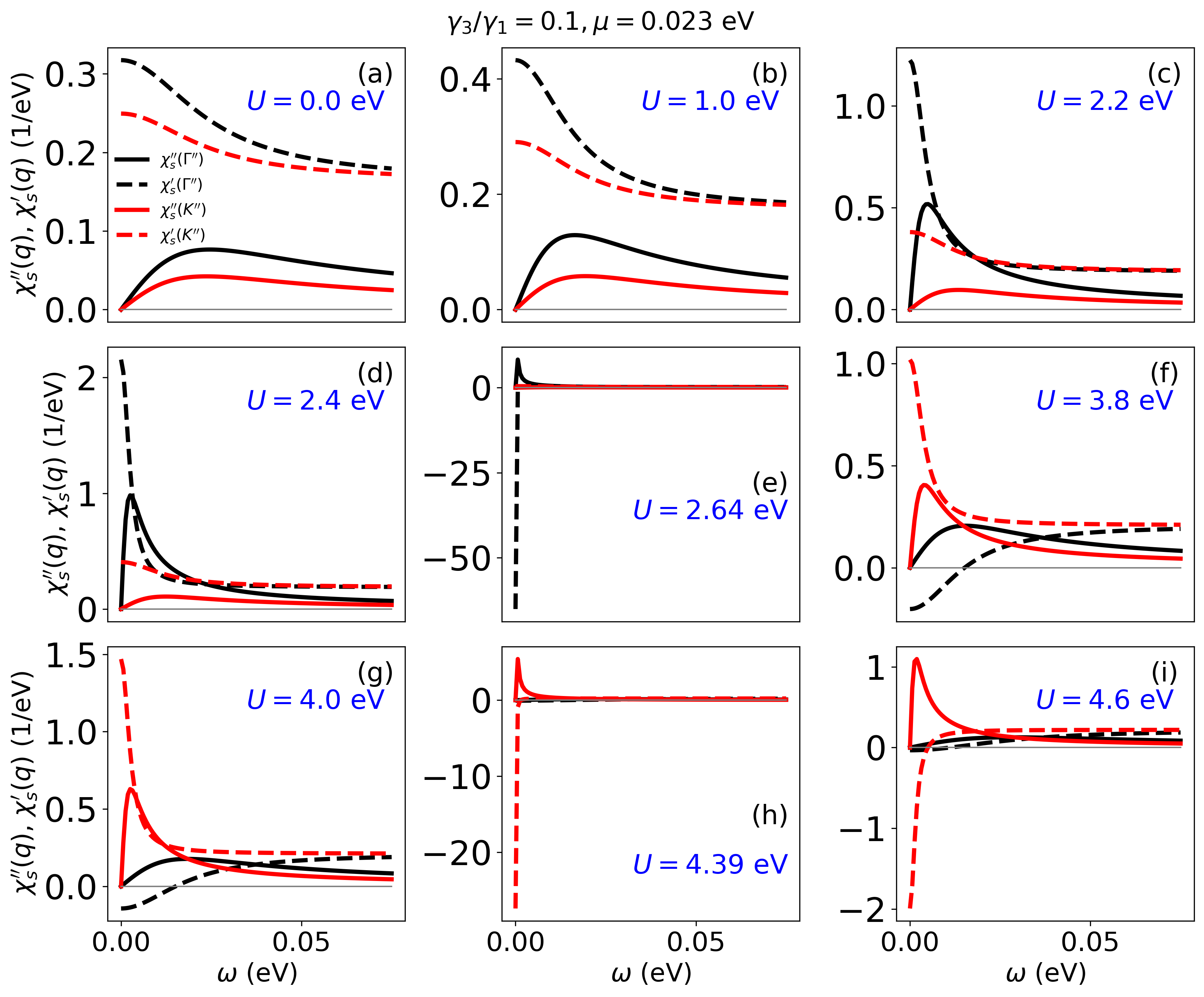
At low interaction strengths , we find qualitatively similar behavior compared to Fig. S4 for the real and imaginary parts of the dynamical spin susceptibility, see Figs. S5(a,b,c,d). A positive peak starts forming for the real part close to , while the imaginary part tends towards a resonance peak once increases. This trend is somewhat more visible for case as compared to . We then find that changes its sign from positive to negative, passing through a negative divergence at eV, see Fig. S5(e). This marks a transition to the ordered state referred to as -FiM in the main text. However, we do not find a clear resonance peak in or clear discontinuous jumps in beyond the transition point, as we did in the half-filled case. The peak in exists but is not very pronounced, while rather smoothly changes its sign from positive to negative values at a finite for , see Figs. S5(e,f,g). Still, the real part crosses zero at the same finite where the imaginary part exhibits a peak. This is similar to the half-filled case, where the zeros of the real part coincide with the resonance peak of the imaginary part. However, altogether this marks notable differences in the spin susceptibility for the -FiM order at finite doping compared to the -FiM order at half-filling, in addition to the different nesting vectors. Similar features are noticed at , where exhibits a negative divergence at eV, see Fig. S5(h), signaling the onsite of the -FiM order. For the real part again crosses zero at a finite exactly where the imaginary part exhibits a faint peak, see Fig. S5(i).
The notably different behavior of the dynamical spin susceptibility beyond the ordering transitions at finite doping compared to the half-filing case beyond the can be explained by damping, which is substantial in the former case. To be precise, the behavior of the dynamic spin susceptibility is connected to the underlying spin-spin relaxation time of the ordered phase. The flattened (sharp) nature of the imaginary part and the smooth (discontinuous) zero-energy crossing of the real part in the ordered states is due to a smaller (larger) value of the spin-spin relaxation time for finite (zero) doping Barra and Hassan (2005); Yalçın (2013). The analysis presented in Figs. S4 and S5 infers that the FiM order at finite doping has a much shorter spin-spin relaxation time. We attribute this behavior to Landau damping associated with the metallic surface state at finite doping, which enhances the spin-spin relaxation rate broadening the magnetic resonance peak as also observed in other RPA studies Maier and Okamoto (2023). Notably, the co-existing Dirac bulk spectrum, also present at half-filling, does not generate any substantial damping.
Finally, we discuss the spin gap for the -FiM orders. In Figs. S6 and S7, we plot the imaginary part of the dynamical spin susceptibility as a function of the repulsion for the nesting vectors that generate the lowest critical Hubbard parameters extracted in Fig. 4, i.e. and , respectively. Note that change as a function of doping, as also indicated in the labels. We also mark the resonance peak in the ordered states with black dots, which denotes the extracted spin gap. At half-filling, panel (a) in both figures, the spin gaps for the -sFM and -sFM orders are visible for zero and small , but they close already at eV, as discussed in the main text, marking the end of the sFM orders. Note that the array of the black dots is nothing but the bright trail in Figs. 2(b,d). The situation changes dramatically as soon as one turns on a finite . At finite doping, panels (b-j), there is no bright trail in the imaginary spin susceptibility at finite and low -values. Instead, we see a sharp peak, almost circular, region develops at the values indicated with thin grey lines. There is thus no spin gap or ordering for . For we find a faint peak, primarily visible through the extracted black dots, emanating from the peak region and increasing in energy for all explored values. We observe the same qualitative behavior for all values of finite doping considered and at both -and nesting vectors. This suggests that once the -and -FiM orders are established at finite , they remain with a finite spin gap. This is markedly different from the half-filled scenario where flat band-mediated commensurate sFM orders exist at zero but are terminated at finite . As such, the -FiM orders at finite doping are more similar to the incommensurate -FiM orders on-setting at finite and not the -sFM orders originating at zero , despite the discrepancy in values between the former pair.
These above results all support the results of Fig. 4 in the main text. In Sec. S5, we discuss the accompanied real-space pattern of the spin moments on the surface of the ABC-MLG.
S5 Magnetic spin textures
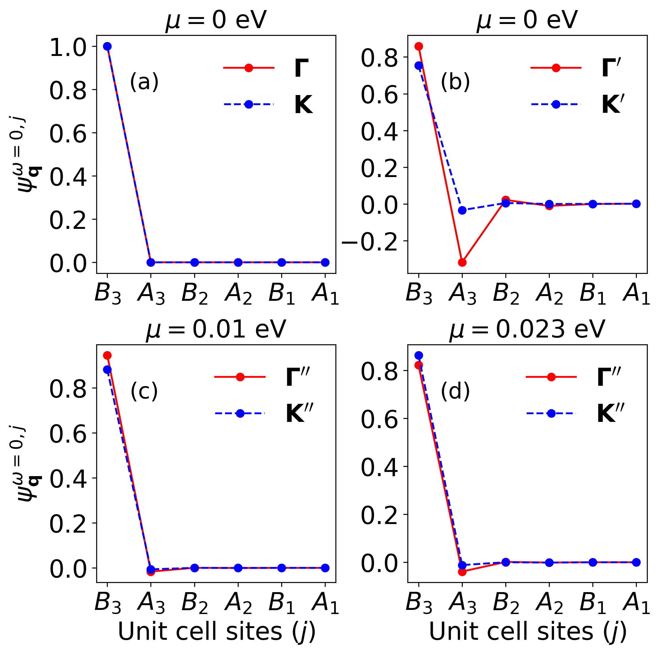
In the main text we discussed and reported data on the magnetic textures, or structure for the sFM orders at half-filling zero and low in section “Flat bands and nesting” and the FiM states in section “FiM order with interactions” for half-filling and in section “Finite doping” away from half-filling. In this SM section, we provide additional information supporting those results and naming conventions. We can access the magnetic textures by investigating the orbital resolved magnetic moment from the eigenvector, , associated with the static susceptibility matrix at its divergence, which marks the transition to magnetic ordering Boehnke (2015). We note, however, that these density-density elements in the eigenvector only carry information about the relative distribution of the magnetic moment across the orbitals in a normalized fashion, while the determination of the exact value of the magnetic moment is not straightforward Boehnke (2015); Christensen et al. (2016); Fong et al. (2000); Gao et al. (2010). Below we start by extracting the magnetic texture in the lattice unit cell (here the surface unit cell) and then comment on the real space texture beyond that.
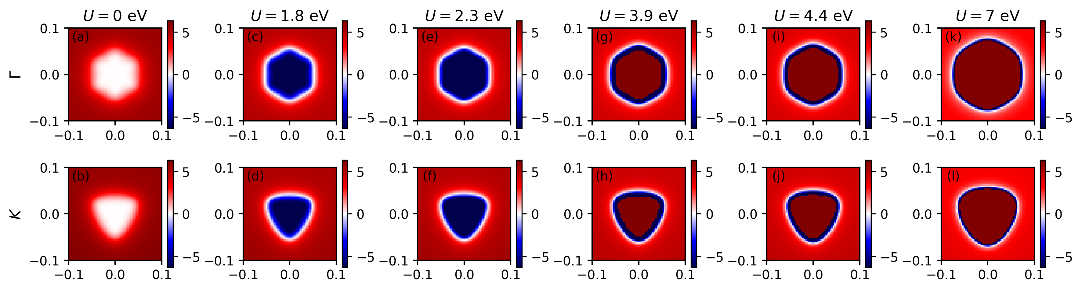
In Fig. S8 we report the distribution of over the orbitals (carbon sites) in the effective surface unit cell we use for our calculations, where and are the atoms of the very top graphene layer. As we find that the imaginary parts of these elements are identically zero, we thus left with the real part that we display. In Fig. S8(a) we study the sFM states at and half-filling and therefore just use the bare static susceptibility at half-filling. From the individual breakdown of the density-density elements in , we find that except the element , all other elements vanish. This generates what we refer to as a sublattice ferromagnetic (sFM) order in the very top graphene layer as there exists no opposite spin moment from element and no moments on any subsurface graphene layers either. In Fig. S8(b) we study the FiM states appearing at finite at half-filling, again plotting the density-density elements in as a function of the six orbitals in the lattice unit cell. Here we find that both the and elements show finite values, with positive and negative intensities, respectively. This marks an antialignment behavior of the moments and due to the strong sublattice polarization, we call this a ferrimagnetic (FiM) order. We repeat the above analysis for doping away from half-filling using the representative values of eV and eV in Figs. S8(c,d), respectively. Note that we here must consider different nesting vectors and for the different values of . Again, the element shows a substantially high value, but also the element is non-zero in both cases and increases with increasing doping. We therefore also refer to these as FiM states, although we note that they are structurally relatively similar to the sFM states as well. Further note that the orderings in each panel in Fig. S8 host different incommensurability and that the -orders also have an extended unit cell.
Finally, we extract the full spatial dependence of the magnetic spin texture. For the -centered orders this magnetic texture extracted in Fig. S8 gives the complete texture as that order is just repeated in each unit cell. For the -orders we need to also consider the incommensurability, which adds real-space modulation to the order. Due to the small amount of incommensurability, this modulation will be very long-range. In Fig. 2(d) in the main text we plot the spatial magnetic texture of the -FiM order, ignoring the incommensurability which due to its long-range modulation is not noticeable on the displayed length scale.
For the -order, the scattering -vector dictates an extended unit cell. We can numerically extract the magnetic texture at all sites in the lattice by taking the real part of the Fourier-transformed density-density elements of the susceptibility eigenvector on the top surface () of ABC-MLG:
| (S1) |
where is the position of the sublattice site in the (original) lattice unit cell. Applying Eq. (S1) we find that all orders trivially repeat with periodicity of the lattice, while the orders result in a extended unit cell. Numerically, we find that the spin densities in the extended unit cell is zero, but time-reversal symmetry is broken, suggesting either a ferrimagnetic or an altermagnetic order. The previously shown dynamic susceptibility maps do not present the altermagnet characteristic two-peaked structure due to the chiral magnons Maier and Okamoto (2023); Šmejkal et al. (2023), establishing the order as zero-magnetization ferrimagnetic state. At realistic and finite doping, incommensurate nesting breaks the perfect zero net magnetization, transforming these states into finite-magnetization FiM states. In the inset of Fig. 3(b) in the main text we plot the resulting magnetic texture for the -FiM order. Again, we here ignore the slight incommensurability which would generate a long-range additional modulation not visible on the length scales plotted in Fig. 3. We here only consider the real part of Eq. (S1) to maintain the condition, which is required for the lattice unit cell.