On Achievable Rates for the Shotgun Sequencing Channel with Erasures

Abstract

In the shotgun sequencing channel, the input sequence (possibly, a long DNA sequence composed of nucleotide bases) is read into multiple fragments (called reads) of much shorter lengths. In the context of DNA data storage, the capacity of this channel was identified in a recent work, assuming that the reads themselves are noiseless substrings of the original sequence. Modern shotgun sequencers however also output quality scores for each base read, indicating the confidence in its identification. Bases with low quality scores can be considered to be erased. Motivated by this, we consider the shotgun sequencing channel with erasures, where each symbol in any read can be independently erased with some probability $\delta$. We identify achievable rates for this channel, using a random code construction and a decoder that uses typicality-like arguments to merge the reads.

I Introduction

Due to its exceptional stability, DNA molecules show great promise as a medium for long term storage of digital data. In the past decade, there has been considerable academic interest in studying and developing DNA as an archival storage medium. This includes practical demonstration of DNA as a storage medium [1] and potential automation of the storage pipeline [2]; characterization of errors in the DNA storage pipeline [3], including in silico simulation of errors due to decay of the molecule [4]; developing algorithms for sequencing of DNA molecules and alignment of reads [5, 6]; developing error-correction codes for DNA storage [7, 8, 9]; and, information theoretic characterization and analysis of DNA storage [10, 11, 12, 13, 14, 15, 16, 17, 18, 19, 20].

These advancements, as well as the academic and industrial interest, in DNA storage have been fuelled by the developments in sequencing techniques which reduced costs and increased feasibility of such storage systems. One such significant development is that of the high-throughput shotgun sequencing pipeline. Rather than sequencing the long DNA sequence in its entirety, which is very expensive and often impractical, multiple copies of the DNA molecule are first created, and then broken into fragments using restriction enzymes. The fragments are generally much shorter in length than the original molecule. These fragments are then sequenced, resulting a collection of reads. The reads are subsequently aligned, by mapping the overlaps between them, to reconstruct the original sequence.

In many modern sequencers, each nucleotide that is sequenced would be accompanied by a quality score, for instance Phred scores[21], corresponding to the probability that the base call for that nucleotide is erroneous. By applying a suitable threshold on the score value, we can treat base calls with scores below the threshold as erasures. Considering the availability of such quality scores, recent works on the information theoretic characterization of the DNA storage channel (for instance, [22, 23]) have considered the low-quality base calls as erasures in the reads.

The work by Lander and Waterman [24] was one of the early ones to analytically model the problem of DNA sequence assembly and derive various limits on the parameters that govern the sequencing, such as the read length and the coverage, for reliable reconstruction. Building on the model developed in [24], Motahari et al. [10] studied the shotgun sequencing channel from an information theoretic perspective. In this work, the length of reads was considered to scale as $\bar{L}\log{n}$, where $\bar{L}$ is a fixed constant and $n$ is the length of the input sequence $\underline{x}$, which was assumed to be generated uniformly at random from all possible quaternary sequences. The work [10] demonstrated some necessary and sufficient conditions on $\bar{L}$, as well as a parameter known as the coverage depth $c$ (which captures the average number of times any position in $\underline{x}$ occurs in the collection of reads), for the reconstruction of $\underline{x}$ in the asymptotic regime, i.e., when $n\to\infty$.

The approach taken in [10] also proved useful in studying the fundamental limits of DNA data storage, where the goal is to find the capacity of the DNA sequencing channel, i.e., the largest normalized size of any collection of input sequences which can be decoded with vanishing error when transmitted through a DNA sequencing channel. For instance, the works [14, 20] identified the capacity of the Sampling-Shuffling Channel, where data is stored as a set of short DNA strands of equal length and reads are obtained by sampling (with replacement) from this set. The capacities of noisy versions of this channel, with errors and erasures, were also presented in [20]. The capacity of the Shotgun Sequencing Channel (with binary-valued inputs) was presented in [12]. In this work [12], $K$ reads of fixed length $L=\bar{L}\log{n}$ are obtained by uniformly sampling their starting positions from the indices of $\underline{x}$. The capacity of this channel was shown to be $(1-e^{-c(1-1/{\bar{L}})})$, where $c=\frac{KL}{n}$ denotes the coverage depth. The achievability in [12] is obtained essentially via a random coding argument, where the decoding algorithm can be seen as a ‘typicality’-based alignment algorithm applied on the reads. A matching converse result is obtained using a genie-aided argument, using the idea of ‘islands’, which refers to maximal collections of reads which overlap with each other. Results from an earlier work [17] on the so-called torn paper channel were used in proving the converse in [12].

In this work, we consider the shotgun sequencing channel with erasures, motivated by the need to incorporate the availability of quality scores of the bases sequenced. The model is similar to that in [12], with the addition being that each symbol in each read is assumed to be erased with probability $\delta$. We denote this channel as $\mathsf{SSE}(\delta)$ (thus, $\mathsf{SSE(0)}$ is the channel considered in [12]). In this work, we obtain an achievability result for the channel $\mathsf{SSE}(\delta)$, thus showing an lower bound on its capacity. The mathematical techniques adopted to show the achievability and the converse results generally follow those in [12]. However, there are differences that arise. In some parts, we are able to simplify the analysis as compared to [12]. In other parts, the analysis is more complicated, owing to the fact that we have to account for the erasures in the reads.

Notation: In this work, ordered tuples or strings are denoted with underlines, such as $\underline{x}$. We denote the set of integers $a,a+1,\ldots,b$ as $[a:b]$. The set of integers $[1:b]$ is denoted as $[b]$. For an event $A$, the indicator random variable associated with the event is denoted by $\mathbb{I}_{A}$. The probability of an event $A$ is denoted by $\Pr(A)$. The complement of an event $A$ is denoted by $\overline{A}$. For two events $A,B$, we write $\Pr(A,B)$ for the probability $\Pr(A\cap B)$. The binomial coefficient is denoted by $\binom{n}{k}$. For a set $S$, the set of finite length strings with symbols from $S$ is denoted by $S^{\star}$.

II Channel Description and Main Result

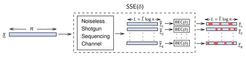
Figure 1: The Shotgun Sequencing Channel with Erasures ($\mathsf{SSE}(\delta)$). The collection ${\cal\tilde{Y}}=\{\tilde{\underline{y}}_{1},\tilde{\underline{y}}_{2},\cdots,\tilde{\underline{y}}_{K}\}$ may be visualized as the output of the Shotgun Sequencing Channel [12], and ${\cal Y}=\{\underline{y}_{1},\underline{y}_{2},\cdots,\underline{y}_{K}\}$ is the output of $\mathsf{SSE}(\delta)$, after bits in each read are erased (indicated in bold/red) with probability $\delta$.

We follow the description and terminology similar to those in [12], as the present work essentially extends the achievability result in [12] for the erasure scenario.

The channel takes an $n$-length binary string $\underline{x}=(x_{1},\ldots,x_{n})\in\{0,1\}^{n}$ as input, corresponding to a message $W\in[2^{nR}]$ chosen at random. The output of the channel can be envisioned as a concatenation of two stages, as shown in Fig. 1. Firstly, the channel samples $K$ substrings of length $L$, from $\underline{x}$. We denote these by a multiset $\tilde{\cal Y}=\{\tilde{\underline{y}}_{1},\ldots,\tilde{\underline{y}}_{K}\}$. Each read $\tilde{\underline{y}}_{i}$ is obtained by first selecting a position ${\mathsf{S}}({\tilde{\underline{y}}_{i}})$ uniformly at random from $[n]$, and then taking the $L$-length (contiguous) substring from the position ${\mathsf{S}}({\tilde{\underline{y}}_{i}})$ onwards, i.e., $\tilde{\underline{y}}_{i}=(x_{{\mathsf{S}}({\tilde{\underline{y}}_{i}})},\ldots,x_{{\mathsf{S}}({\tilde{\underline{y}}_{i}})+L-1})\in\{0,1\}^{L}$. When ${\mathsf{S}}({\tilde{\underline{y}}_{i}})>n-L+1$, similar to the circular DNA model in [10], we assume that the substring is obtained in a cyclic wrap-around fashion, for ease of analysis. Thus, $\tilde{\cal Y}$ can be thought of as the output of a noise-free shotgun sequencing channel (as in [12]), when the input is $\underline{x}$.

In the second stage, each read $\tilde{\underline{y}}_{i}$ is assumed to pass through a binary erasure channel with erasure probability $\delta$ (denoted by $\mathsf{BEC}(\delta)$, thus erasing each position in $\tilde{\underline{y}}_{i}$ with probability $\delta$ independently, to obtain $\underline{y}_{i}\in\{0,1,\perp\}^{L}$, where $\perp$ denotes an erasure. The multiset of these reads, denoted as ${\cal Y}=\{\underline{y}_{i}:i\in[K]\}$, is the output of the channel. Note that the start positions are unaltered, i.e., ${\mathsf{S}}({\underline{y}_{i}})={\mathsf{S}}({\tilde{\underline{y}}_{i}}),\forall i$. We denote this shotgun sequencing channel with erasures as $\mathsf{SSE}(\delta)$.

A rate $R$ is said to be achievable if the message $W$ can be reconstructed from ${\cal Y}$ using some decoding algorithm with a probability of error that is vanishing as $n$ grows large. The capacity of the $\mathsf{SSE}(\delta)$ is then defined as $C_{\mathsf{SSE}(\delta)}\triangleq\lim_{n\to\infty}\sup\{R:R~{}\text{is achievable}\}$.

The expected number of times a coordinate of $\underline{x}$ (say the $j^{\texttt{th}}$ coordinate) is sequenced in the first stage is called the coverage depth, denoted as $c$. Thus, $c\triangleq\mathbb{E}(\sum_{i=1}^{K}\mathbb{I}_{\{j\in[{\mathsf{S}}({\underline{y}_{i}}):{\mathsf{S}}({\underline{y}_{i}})+L-1]\}}).$ A simple calculation reveals that

$$c=\frac{KL}{n}$$ (1)

We assume that the length of each read is $L=\Theta(\log{n})\triangleq\bar{L}\log{n}.$ for some positive $\bar{L}$. As in [12], we study the regime where $c$ and $\bar{L}$ are some positive constants. Thus in our regime, $K=\frac{cn}{\bar{L}\log{n}}=\Theta\left(\frac{n}{\log{n}}\right).$

In this work, we obtain an upper bound for $C_{\mathsf{SSE}(\delta)}$, via a random code construction, and a decoder which uses typicality-like techniques for estimating the true message. The main result in this work is the following.

Theorem 1

Let $c$ and $\bar{L}$ be the parameters of the $\mathsf{SSE}(\delta)$ such that $c>0$ and $\bar{L}(1-\delta)>1$. Let $\alpha=c/(\bar{L}(1-\delta))$. For any $d>0$, the rate $R$ is achievable on the $\mathsf{SSE}(\delta)$ channel if

$$R<\left(1-e^{-c(1-\delta)}\right)-\frac{ce^{-c}}{\bar{L}}-\upbeta(d),$$ (2)

where

$$\upbeta(d)=\frac{d}{(1-\delta)}\cdot\left(\frac{c}{\bar{L}}\right)^{2}\cdot e^{-c}\cdot\left(\frac{e^{\alpha d}(e^{\alpha}-1)}{(e^{\alpha d}-1)}\right.\left.\frac{e^{2\alpha d}\left(\left(e^{\alpha(1+d)}-e^{\alpha}\right)-d\left(e^{\alpha(1+d)}-1\right)\right)}{\left(e^{\alpha d}-1\right)^{2}}\right).$$

Remark 1

The quantity $d$ and the unwieldy expression for $\upbeta(d)$ is due to the arguments used in the proof. Simulation results show that the value of $\upbeta(d)$ decreases as $d$ reduces, and thus the expression $\upbeta(d)$ likely converges as $d\to 0$. However, we are currently unable to prove this analytically.

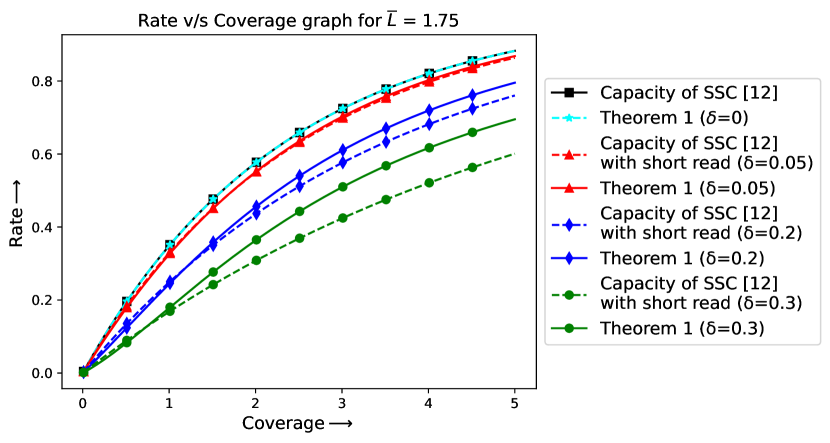
Figure 2: The plot shows comparison of the rate from Theorem 1, with $\bar{L}=1.75$, as the coverage depth $c$ varies, for $\delta=0,0.05,0.2,$ and $0.3$. These are compared with results from [12].

Fig. 2 plots the upper bound for the achievable rate for $\mathsf{SSE}(\delta)$ from Theorem 1, for $\delta\in\{0,0.05,0.2,0.3\}$, against varying values for the coverage depth $c$. The parameter $\bar{L}$ is fixed as $1.75$ (thus satisfying the requirement $\bar{L}(1-\delta)>1$, for all chosen $\delta$). The parameter $d$ is fixed as $10^{-6}$. For comparison, we also plot the capacity of the shotgun sequencing channel (SSC) from [12], i.e., the expression $(1-e^{-c(1-1/{\bar{L}})})$. We observe that, when $\delta=0$, our bound from Theorem 1 appears identical to the capacity of the SSC.

As another note of comparison, we also plot the SSC capacity from [12], with shortened reads of size $\bar{L}(1-\delta)\log n$ (note that the read length is $\bar{L}\log n$ in $\mathsf{SSE}(\delta)$). We observe that this short-read SSC capacity is larger than our bound from Theorem 1, when $c$ is small ($c<1$), whereas it is progressively smaller compared to our bound, as $c$ increases (for given $L$, this means $K$ increases). We remark why this may be the case. Firstly, we observe that, due to the length being shorter, the number of reads $K$ for the SSC is smaller than $K$ for the $\mathsf{SSE}(\delta)$, for any specific $c$. In spite of this, for larger values of $c$, some information about the relative positions of the bits in the transmitted sequence is likely lost by the SSC, as the read length is shorter. The $\mathsf{SSE}(\delta)$ channel is probably able to preserve the information about the relative positions better, due to the longer reads, in spite of the erasures and lesser $K$. In the small $c$ regime, there are likely too few reads in $\mathsf{SSE}(\delta)$ to see this advantage. Instead, due to $K$ being less, the reconstructed sequence in $\mathsf{SSE}(\delta)$ likely has many unrecoverable bits, compared to the SSC channel (in spite of its shortened reads).

III Achievablity

We use a random coding argument to show the achievability of the rate as in Theorem 1. We outline the main components of our code design below. While these share similarities to the techniques in [12], the decoding algorithm and the proof arguments are more complex, owing to consideration of the reads with erasures.

III-A Outline of the Coding Scheme

• Codebook: A codebook with $2^{nR}$ codewords, denoted as ${\mathcal{C}}=\{\underline{x}_{1},\underline{x}_{2},\cdots,\underline{x}_{2^{nR}}\}$, is generated by picking each symbol of $\underline{x}_{j}$ independently and uniformly at random from $\{0,1\}$, for each $j\in[2^{nR}]$.

• Encoder: To communicate the message $W$ (chosen uniformly at random from $[2^{nR}]$) through the channel $\mathsf{SSE}(\delta)$, the encoder communicates the codeword $\underline{x}_{W}\in{\mathcal{C}}$ through the channel. The output $\cal Y$, a set of reads as described in Section II, is generated post-sequencing.

• Decoder: The decoding algorithm we propose takes as input the collection of reads ${\cal Y}$ and generates an estimate $\hat{W}$ of the transmitted message, or a failure. We briefly describe the process of obtaining the estimate $\hat{W}$ from ${\cal Y}$. The decoder proceeds in three phases. In the first phase, which we call the merge phase, the decoder first implements a merging process of the reads. Such a merging process will be run for all possible orderings of the reads, considering multiple possible ‘typical’ ways to merge the reads, where the typicality will be defined based on the concentration properties of some quantities we will subsequently define.

  For each such typical merge process, we get a set of islands, where an island refers to a string of maximal length obtained in the merging process (formal definitions follow in subsequent subsections). Ultimately, upon going through all possible orderings, several such island sets may be generated. In the second phase, which we call the filtering phase, these island sets are then filtered based on further typicality constraints. The filtered island sets which pass the final typicality conditions are referred to as candidate island sets. The third and final phase is called the compatibility check phase. In this phase, for each candidate island set, the decoder checks if all the islands of that candidate island set occur as compatible substrings of any codeword. If there is precisely one codeword $\underline{x}_{\hat{w}}$ in $\cal C$ that passes this check, across all the candidate island sets, then the estimate is declared as $\hat{W}=\hat{w}$. Otherwise, a decoding failure is declared. We show that the decoding algorithm results in the correct estimate, i.e., $W=\hat{W}$ with high probability, as $n$ grows large. A more precise description and analysis of the decoding is provided in Subsection III-D and III-F. Subsection III-B and Subsection III-C describe the various quantities required for the description and analysis of the decoder, and the concentration results on some of these quantities, respectively.

III-B Merging and Coverage: Definitions and Terminology

We now give the formal definitions and terminology for various quantities. Again, these quantities are either identical or parallel to those defined in [12].

Definition 1 (Length and Size of string)

For any $\underline{u}\in\{0,1,\perp\}^{\star}$, the length of $\underline{u}$ is denoted by ${\ell}(\underline{u})$. The size of $\underline{u}$ is the number of unerased bits in $\underline{u}$ and is denoted by ${\ell}_{ue}(\underline{u})$.

Definition 2 (Prefix and Suffix)

For a string $\underline{v}\in\{0,1,\perp\}^{l}$ and any positive integer $l^{\prime}\leq l$, a string $\underline{z}\in\{0,1,\perp\}^{l^{\prime}}$ is said to be a $l^{\prime}$-suffix of $\underline{v}$, if $(v_{l-l^{\prime}+1},\ldots,v_{l})=\underline{z}$, and is denoted by $\texttt{suffix}(\underline{v},l^{\prime})$. Similarly, if $(v_{1},\ldots,v_{l^{\prime}})=\underline{z}$, then $\underline{z}$ is said to be a $l^{\prime}$-prefix of $\underline{v}$ and is denoted by $\texttt{ prefix}(\underline{v},l^{\prime})$.

Definition 3 (Compatibility, $l$-compatible strings and substring compatibility)

Let $\underline{u}$ and $\underline{v}$ be any two strings in $\{0,1,\perp\}^{l}$. We say that $\underline{v}$ and $\underline{u}$ are compatible, if

$$u_{i}=\perp~{}\text{or}~{}v_{i}=\perp,~{}~{}~{}\text{for any }~{}i\in[l]~{}\text{s.t.}~{}u_{i}\neq v_{i}.$$

For any $\underline{u},\underline{v}\in\{0,1,\perp\}^{\star}$ (not necessarily of same length), the string $\underline{v}$ is said to be a compatible substring of $\underline{u}$, if $\underline{v}$ is compatible with any substring of $\underline{u}$. Finally, for any $\underline{u},\underline{v}\in\{0,1,\perp\}^{\star}$, we say $\underline{v}$ is $l$-compatible with $\underline{u}$, if $\texttt{suffix}(\underline{u},l)$ and $\texttt{ prefix}(\underline{v},l)$ are compatible.

We define the merging of two reads in the following manner.

Definition 4 (Merge of two strings)

Let $\underline{u}$ and $\underline{v}$ be any two strings in $\{0,1,\perp\}^{\star}$ such that $\underline{v}$ is $l$-compatible with $\underline{u}$. Let $\texttt{suffix}(\underline{u},l)=\underline{u}^{\prime}$ and $\texttt{ prefix}(\underline{v},l)=\underline{v}^{\prime}$. Suppose ${\ell}_{ue}(\underline{u}^{\prime})\neq 0$. Then, we say that $\underline{u}$ and $\underline{v}$ are mergeable with overlap $l$. The output of the merge operation is defined as the string obtained by the concatenation of three substrings: $\underline{u}^{\prime\prime}$, $\underline{z}$ and $\underline{v}^{\prime\prime}$, where $\underline{u}^{\prime\prime}=\texttt{ prefix}(\underline{u},{\ell}(\underline{u})-l)$, $\underline{v}^{\prime\prime}=\texttt{suffix}(\underline{v},{\ell}(\underline{v})-l)$, and $\underline{z}$ is defined as follows.

$$z_{i}=\begin{cases}0&\text{if }u_{i}^{\prime}=0\text{ or }v_{i}^{\prime}=0,\\ 1&\text{if }u_{i}^{\prime}=1\text{ or }v_{i}^{\prime}=1,\\ \perp&\text{if }u_{i}^{\prime}=\perp\text{ and }v_{i}^{\prime}=\perp\end{cases}.$$

With respect to the merge defined above, we term the substring $\underline{u}^{\prime}$ as the merging suffix, or simply the suffix. Fig. 3 shows an illustration of this merge operation.

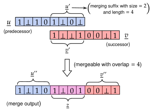
Figure 3: Illustration of a merge operation.

We also recall that, during the sequencing process, each of the read $\underline{y}\in{\cal Y}$ has a certain starting position ${\mathsf{S}}({\underline{y}})$. The following terminologies are regarding the ground truth of ${\cal Y}$.

Definition 5 (True Successors, Ordering, and Overlaps)

The true successor of a read $\underline{y}_{1}\in{\cal Y}$ is a read $\underline{y}_{2}\in{\cal Y}$, such that ${\mathsf{S}}({\underline{y}_{2}})\geq{\mathsf{S}}({\underline{y}_{1}})$ (in cyclic wrap around fashion) and $({\mathsf{S}}({\underline{y}_{2}})-{\mathsf{S}}({\underline{y}_{1}}))$ is smallest among all reads $\underline{y}_{2}\in{\cal Y}$. Thus, the true ordering, is an ordering of the $K$ reads such that each read is succeeded by its true successor. The true overlap between any read $\underline{y}_{1}$ and its true successor $\underline{y}_{2}$ is defined to be $0$, if ${\mathsf{S}}({\underline{y}_{2}})>{\mathsf{S}}({\underline{y}_{1}})+L-1$ (in cyclic wrap around manner). If ${\mathsf{S}}({\underline{y}_{1}})\leq{\mathsf{S}}({\underline{y}_{2}})\leq{\mathsf{S}}({\underline{y}_{1}})+L-1$, then the true overlap of $\underline{y}_{1}$ with $\underline{y}_{2}$ is ${\mathsf{S}}({\underline{y}_{1}})+L-{\mathsf{S}}({\underline{y}_{2}}).$

As mentioned before, our algorithm merges the reads corresponding to various orderings and typical overlaps. We now formally define the notion of an island arising out of a merging process of the reads, following a given ordering and a tuple prescribing the overlaps.

Definition 6 (Orderings, Islands, and True Islands)

Let $\upzeta$ denote a permutation of $[K]$. Consider the ordering of the $K$ reads defined by $\upzeta$. With respect to this ordering, the read $\underline{y}_{\upzeta(i)}$ is called the predecessor of the read $\underline{y}_{\upzeta(i+1)}$, while $\underline{y}_{\upzeta(i+1)}$ is the successor of $\underline{y}_{\upzeta(i)}$. Consider $\underline{\omega}=(\omega_{1},\ldots,\omega_{K})\in[0:L]^{K}$. For some $j\in[K]$, for some positive integer $l$, suppose that the following conditions hold.

• $\omega_{j^{\prime}}>0$ and $\underline{y}_{\upzeta(j^{\prime})}$ is mergeable with $\underline{y}_{\upzeta(j^{\prime}+1)}$ with size of the suffix being $\omega_{j^{\prime}}$, for all $j^{\prime}\in[j:j+l-1]$ (in cyclic wrap around fashion).

• $\omega_{j-1}=\omega_{j+l}=0$.

Then the string obtained by the merging of the reads $\underline{y}_{\upzeta(j^{\prime})}:j^{\prime}\in[j:j+l-1]$ successively with their respective successors, is called an island. If $\upzeta^{t}$ is the true ordering of the reads, and each read $\underline{y}$ is merged with its successor $\underline{y}^{\prime}$ (as per $\upzeta^{t}$) based only on the true overlap, i.e., if ${\mathsf{S}}({\underline{y}})+L-{\mathsf{S}}({\underline{y}^{\prime}})>0$, then the islands so obtained are called true islands.

Another quantity that will use to check the goodness of our islands is the expected number of unerased bits in them. Towards that end, we have the following two definitions.

Definition 7

(A bit being covered and visibly covered): The $i^{\texttt{th}}$ bit of $\underline{x}_{W}$, denoted by $x_{i}$, is said to be covered by a read $\underline{y}\in{\cal Y}$ if ${\mathsf{S}}({\underline{y}})\in[i-L+1:i]$. Further, $x_{i}$ is said to be visibly covered by $\underline{y}$ if it is covered by $\underline{y}$ and further unerased in $\underline{y}$. The bit $x_{i}$ is said to be covered (visibly covered) by the collection of reads ${\cal Y}$ if it is covered (visibly covered, respectively) by at least one read in ${\cal Y}$.

Definition 8 (Coverage and Visible Coverage)

The coverage, denoted by $\Phi$ (visible coverage, respectively, denoted by $\Phi_{v}$) $\Phi$ of the collection ${\cal Y}$ is defined as the fraction of the bits which are covered (visibly covered, respectively) by the reads in ${\cal Y}$. Thus, $\Phi\triangleq\frac{1}{n}\sum_{i=1}^{n}\mathbb{I}_{\{x_{i}\text{ is covered by reads in }{\cal Y}\}}$ and $\Phi_{v}\triangleq\frac{1}{n}\sum_{i=1}^{n}\mathbb{I}_{\{x_{i}\text{ is visibly covered by reads in }{\cal Y}\}}.$

To analyse the errors the decoder can make while merging, we need to bound the different possible ways a read can be merged with other reads in the set $\cal Y$. To capture this, we define the quantity $M_{\underline{z}}$.

Definition 9 (The quantity $M_{\underline{z}}$)

For a string $\underline{z}=\{0,1,\perp\}^{l},l\in[L]$, random variable $M_{\underline{z}}$ is defined as the number of reads in ${\cal Y}$, which are $l$-compatible with $\underline{z}$ (i.e., has a $l$-length prefix that is compatible with $\underline{z}$). Thus,

$$M_{\underline{z}}\triangleq\sum_{\underline{y}\in{\cal Y}}\mathbb{I}_{\{\underline{y}\text{ is $l$-compatible with }\underline{z}\}}$$

Towards assessing the goodness of some overlap tuples, we need the following quantity, denoted by $G(\tau)$.

Definition 10 (The quantity $G(\tau)$)

We define $G(\tau)$ to be the number of reads in ${\cal Y}$, such that for each such read, the size of the merging suffix with its true successor is $\tau\log{n}$. Thus,

$$G(\tau)\triangleq\sum_{i\in[K]}\mathbb{I}_{\omega^{t}_{i}=\tau\log n},$$ (3)

where $\underline{\omega}^{t}=(\omega_{1}^{t},\ldots,\omega_{K}^{t})$ is the sequence of sizes of the true merging suffixes.

III-C Concentration Results and Bounds on Quantities

In order to show achievability, we will first prove some concentration results for some of the quantities that we have defined. Our first concentration result is on the number of true islands. Note that by definition, erasures do not affect the existence of any true islands. Hence, the proof for the following lemma is identical to the proof of Lemma 2 in [12].

Lemma 1 (Concentration of Number of True Islands)

Let the number of true islands be $K^{\prime}$. Thus, for any $\epsilon>0$

$$\lim_{n\to\infty}\Pr\left(\left|K^{\prime}-Ke^{-c}\right|\geq\epsilon Ke^{-c}\right)=0.$$

We now show the concentration of the visible coverage.

Lemma 2 (Concentration of Visible Coverage)

For any $\epsilon>0$, the visible coverage $\Phi_{v}$ satisfies

$$\lim_{n\to\infty}\Pr\left(|\Phi_{v}-(1-e^{-c(1-\delta)})|>\epsilon(1-e^{-c(1-\delta)})\right)=0.$$ (4)

Proof:

We have the following equalities,

$$\mathbb{E}\left[\Phi_{v}\right] =\frac{1}{n}\cdot\mathbb{E}\left[\sum_{i=1}^{n}\mathbb{I}_{\{x_{i}\text{ is covered by in reads in }{\cal Y}\}}\right]$$

$$=\Pr(x_{1}\text{ is covered by in reads in }{\cal Y})$$

$$=1-\Pr(x_{1}\text{ is not covered by in reads in }{\cal Y})$$

$$=1-\Pr(x_{1}\text{ is not covered by }\underline{y}_{j},\forall j\in\{1,\cdots,K\})$$

$$=1-\Pr(x_{1}\text{ is not covered by read }\underline{y}_{1})^{K}$$

$$=1-(1-\Pr(x_{1}\text{ is covered by read }\underline{y}_{1}))^{K}.$$

Now, $\Pr(x_{1}\text{ is covered by read }\underline{y}_{1})=\frac{L}{n}(1-\delta).$ Hence,

$$\mathbb{E}\left[\Phi_{v}\right] =1-\left(1-\left(\frac{L}{n}(1-\delta)\right)\right)^{K}$$

$$=1-\left(1-\left(\frac{L}{n}(1-\delta)\right)\right)^{\left(\frac{cn}{L}\right)}$$

$$=1-\left(1-\left(\frac{\bar{L}\log n}{n}(1-\delta)\right)\right)^{\left(\frac{cn}{\bar{L}\log n}\right)}.$$

Let $t=\left(\frac{n}{\bar{L}\log n(1-\delta)}\right)$ Hence, we get

$$\lim_{n\to\infty}\mathbb{E}\left[\Phi_{v}\right] =\lim_{t\to\infty}\mathbb{E}\left[\Phi_{v}\right]$$

$$=\lim_{t\to\infty}\left(1-\left(1-\frac{1}{t}\right)^{\left(c(1-\delta)t\right)}\right)$$

$$=1-\lim_{t\to\infty}\left(\left(1-\frac{1}{t}\right)^{\left(c(1-\delta)t\right)}\right)$$ (5)

$$=(1-e^{-c(1-\delta)}).$$ (6)

The rest of this proof follows almost identical arguments as in the Lemma 1 of [12], essentially bounding the variance of $\Phi_{v}$ and using the Chebyshev inequality to complete the result. We therefore omit the details. ∎

Remark 2

Note that the concentration of the coverage $\Phi$ (i.e., Lemma 1 in [12]) also follows from Lemma 2, by substituting $\delta=0$.

Lemma 3 shows the concentration of the parameter $G(\tau)$ in some regime around its mean. Lemma 3 is similar to Lemma 4 in [12], and the proof follows similar arguments. However, a key difference with [12] is that the deviation around the mean in Lemma 4 of [12] is a function of $\bar{G}(\tau)$, whereas for our purpose here, the deviation ${\epsilon n}/{\log^{2}{n}}$ suffices.

Lemma 3

For any $\epsilon>0$,

$$\lim_{n\to\infty}\Pr{\left(\bigcup_{\tau\in{\cal T}}\left\{\left|G(\tau)-\bar{G}(\tau)\right|\geq\frac{\epsilon n}{\log^{2}{n}}\right\}\right)}=0,$$

where ${\cal T}=\{\frac{1}{\log{n}},\frac{2}{\log{n}},\cdots,\bar{L}\}$ and $\bar{G}(\tau)\triangleq\mathbb{E}[G(\tau)]$.

Proof:

We know that,

$$\Pr{\left(\bigcup_{\tau\in{\cal T}}\left\{\left|G(\tau)-\bar{G}(\tau)\right|\geq\epsilon\frac{n}{\log^{2}{n}}\right\}\right)}\leq\frac{\mathrm{Var}{(G(\tau))}}{\epsilon^{2}\cdot\left(\frac{n}{\log^{2}{n}}\right)^{2}}.$$ (7)

Let $A_{i}$ denote the event that the $i^{\texttt{th}}$ read $\underline{y}_{i}$ overlaps with its true successor with size of merging suffix as $\tau\log{n}$. Thus, $G(\tau)=\sum_{i=1}^{K}\mathbb{I}_{A_{i}}$. As the random variables $A_{i}:i\in[K]$ are identically distributed, we have $\bar{G}(\tau)=K\Pr(A_{i})$, for any $i$.

As $G(\tau)$ is the sum of indicator random variables, the following is true (for a proof, see Chapter 4 in [25], for instance),

$$\mathrm{Var}(G(\tau))\leq\bar{G}(\tau)+\sum_{i,j\in[K]:i\neq j}\mathrm{Cov}(\mathbb{I}_{A_{i}},\mathbb{I}_{A_{j}}),$$ (8)

where

$$\mathrm{Cov}(\mathbb{I}_{A_{i}},\mathbb{I}_{A_{j}})=\mathbb{E}[\mathbb{I}_{A_{i}}\mathbb{I}_{A_{j}}]-\mathbb{E}[\mathbb{I}_{A_{i}}]\mathbb{E}[\mathbb{I}_{A_{j}}],$$ (9)

is the covariance between the random variables $\mathbb{I}_{A_{i}}$ and $\mathbb{I}_{A_{j}}$.

Now,

$$\mathbb{E}[\mathbb{I}_{A_{i}}]=\Pr(A_{i})=\frac{\bar{G}(\tau)}{K}=\mathbb{E}[\mathbb{I}_{A_{j}}].$$ (10)

Further, $A_{i}$ and $A_{j}$ are independent if reads $\underline{y}_{i}$ and $\underline{y}_{j}$ do not overlap, i.e., $|{\mathsf{S}}({\underline{y}_{i}})-{\mathsf{S}}({\underline{y}_{j}})|\geq L$. Thus, we have

$$\mathbb{E}[\mathbb{I}_{A_{i}}\mathbb{I}_{A_{j}}] =\Pr(A_{i},A_{j})$$

$$\leq\Pr(A_{i},A_{j}|\{|{\mathsf{S}}({\underline{y}_{i}})-{\mathsf{S}}({\underline{y}_{j}})|\geq L\})$$

$$~{}~{}~{}~{}+\Pr(\{|{\mathsf{S}}({\underline{y}_{i}})-{\mathsf{S}}({\underline{y}_{j}})|<L\})$$

$$\leq\Pr(A_{i})\Pr(A_{j})+\frac{L}{n}$$

$$=\frac{\bar{G}(\tau)^{2}}{K^{2}}+\frac{L}{n}.$$ (11)

Using (9), (10) and (III-C) in (8), we get

$$\mathrm{Var}(G(\tau)) \leq\bar{G}(\tau)+\sum_{i,j\in[K]:i\neq j}\frac{L}{n}$$

$$\leq\bar{G}(\tau)+K^{2}\frac{L}{n}$$ (12)

$$\stackrel{{\scriptstyle(a)}}{{\leq}}K+cK=(1+c)K,$$ (13)

where (a) holds as $G(\tau)\leq K$, by definition. Using (13) in (7),

$$\Pr \left(\bigcup_{\tau\in{\cal T}}\left\{\left|G(\tau)-\bar{G}(\tau)\right|\geq\epsilon\frac{n}{\log^{2}{n}}\right\}\right)\leq\frac{\mathrm{Var}{(G(\tau))}}{\epsilon^{2}\cdot\left(\frac{n}{\log^{2}{n}}\right)^{2}}\leq\frac{(1+c)K}{\epsilon^{2}\cdot\left(\frac{n}{\log^{2}{n}}\right)^{2}}=\Theta\left(\frac{\log^{3}{n}}{n}\right)\to 0,$$

as $n\to\infty$. ∎

Lemma 4 gives us concentration results for the parameter $M_{\underline{z}}$ in various regimes. This is similar to Lemma 3 in [12], except that the proof is simpler than in [12].

Lemma 4

For $\underline{z}\in\cup_{l\in[L]}\{0,1,\perp\}^{l}$, let $\tau_{ue}(\underline{z})={\ell}_{ue}(\underline{z})/\log n$. The following are then true,

1. $\lim_{n\to\infty}\Pr\left(\bigcup_{\underline{z}\colon\tau_{ue}(\underline{z})\leq 1-\epsilon}\left\{\left|M_{\underline{z}}-Kn^{-\tau_{ue}(\underline{z})}\right|\geq\epsilon Kn^{-\tau_{ue}(\underline{z})}\right\}\right)=0.$

2. $\lim\limits_{n\to\infty}\Pr\left(\bigcup_{\underline{z}\colon\tau_{ue}(\underline{z})>1-\epsilon}\{M_{\underline{z}}\geq n^{\epsilon}\}\right)=0.$

Proof:

Consider vectors with erasures of the form $\underline{z}=\{0,1,\perp\}^{l},$ $l\leq L$. For the transmitted codeword $\underline{x}\in\{0,1\}^{n}$, let $D\triangleq\{i\in[n]\colon(x_{i},\cdots,x_{i+l-1})\text{ is $l$-compatible with }\underline{z}\}$. Therefore, $M_{\underline{z}}=\sum_{i=1}^{K}\mathbb{I}_{\{{\mathsf{S}}({\underline{y}_{i}})\in D\}}$. Observe that $\Pr(\mathbb{I}_{\{{\mathsf{S}}({\underline{y}_{i}})\in D\}}=1)=1/2^{\tau_{ue}(\underline{z})\log n}=n^{-\tau_{ue}(\underline{z})}$. Further, the random variables $\mathbb{I}_{\{{\mathsf{S}}({\underline{y}_{i}})\in D\}}:i\in[K]$ are independent, as ${\mathsf{S}}({\underline{y}_{i}}):i\in[K]$ are independent random variables.

We first prove part a). Consider $\tau_{ue}(\underline{z})\leq 1-\epsilon$.

$$\Pr \left(\bigcup_{\underline{z}:\tau_{ue}(\underline{z})\leq 1-\epsilon}\left\{\left|M_{\underline{z}}-Kn^{-\tau_{ue}(\underline{z})}\right|\geq\epsilon Kn^{-\tau_{ue}(\underline{z})}\right\}\right)$$

$$\leq\sum_{\underline{z}:\tau_{ue}(\underline{z})\leq 1-\epsilon}\Pr\left(\left\{\left|M_{\underline{z}}-Kn^{-\tau_{ue}(\underline{z})}\right|\geq\epsilon Kn^{-\tau_{ue}(\underline{z})}\right\}\right)$$

$$\stackrel{{\scriptstyle(a)}}{{\leq}}\bar{L}\log{n}\cdot n^{\bar{L}\log{3}}\cdot$$

$$~{}~{}~{}~{}\max_{\underline{z}:\tau_{ue}(\underline{z})\leq 1-\epsilon}\Pr\left(\left\{\left|M_{\underline{z}}-Kn^{-\tau_{ue}(\underline{z})}\right|\geq\epsilon Kn^{-\tau_{ue}(\underline{z})}\right\}\right)$$

$$\stackrel{{\scriptstyle(b)}}{{\leq}}\bar{L}\log{n}\cdot n^{\bar{L}\log{3}}\cdot 2e^{-\left(\frac{K\cdot n^{-\tau_{ue}(\underline{z})}\epsilon^{2}}{(1-n^{-\tau_{ue}(\underline{z})})}\right)}$$

$$\leq\bar{L}\log{n}\cdot n^{\bar{L}\log{3}}\cdot 2e^{-\left(\frac{c\cdot n^{1-\tau_{ue}(\underline{z})}\epsilon^{2}}{2L}\right)}$$

$$\stackrel{{\scriptstyle(c)}}{{\leq}}\bar{L}\log{n}\cdot n^{\bar{L}\log{3}}\cdot 2e^{-\left(\frac{c\cdot n^{\epsilon}\epsilon^{2}}{2L}\right)}.$$

Here $(a)$ holds as $|\{\underline{z}:\tau_{ue}(\underline{z})\leq 1-\epsilon\}|\leq\sum_{l=1}^{L}3^{l}\leq\sum_{l=1}^{L}3^{L}\leq L\cdot 3^{L}=\bar{L}\log{n}\cdot n^{\bar{L}\log{3}}$. The inequality $(b)$ is from Hoeffding’s inequality in Lemma 5 (which we use with the parameters $X_{i}=\mathbb{I}_{\{{\mathsf{S}}({\underline{y}_{i}})\in D\}}$, $N=K$, and $p=n^{-\tau_{ue}(\underline{z})}$), and $(c)$ follows as $\tau_{ue}(\underline{z})\leq 1-\epsilon$. Thus, part a) of the lemma can be seen to be true, from the R.H.S. of the inequality (c).

Similarly, for $\frac{l}{\log{n}}>1-\epsilon$, we have,

$$\Pr\left(\bigcup_{\underline{z}:\tau_{ue}(\underline{z})>1-\epsilon}\{M_{\underline{z}}\geq n^{\epsilon}\}\right) \leq\bar{L}\log{n}\cdot n^{\bar{L}\log{3}}\max_{\underline{z}:\tau_{ue}(\underline{z})>1-\epsilon}\Pr\left(\{M_{\underline{z}}\geq n^{\epsilon}\}\right)$$

$$\stackrel{{\scriptstyle(a)}}{{\leq}}\bar{L}\log{n}\cdot n^{\bar{L}\log{3}}\cdot e^{-\left(\frac{\left(n^{\epsilon}-Kn^{-\tau_{ue}(\underline{z})}\right)^{2}}{2Kn^{-\tau_{ue}(\underline{z})}(1-n^{-\tau_{ue}(\underline{z})})}\right)}$$

$$\leq\bar{L}\log{n}\cdot n^{\bar{L}\log{3}}\cdot e^{-\left(\frac{\left(n^{\epsilon}-(c/L)n^{1-\tau_{ue}(\underline{z})}\right)^{2}}{2(c/L)n^{1-\tau_{ue}(\underline{z})}}\right)}$$

$$\stackrel{{\scriptstyle(b)}}{{\leq}}\bar{L}\log{n}\cdot n^{\bar{L}\log{3}}\cdot e^{-\left(\frac{\left(n^{\epsilon}-(c/L)n^{\epsilon}\right)^{2}}{2(c/L)n^{\epsilon}}\right)}$$

$$\leq\bar{L}\log{n}\cdot n^{\bar{L}\log{3}}\cdot e^{-\left(\frac{n^{\epsilon}\left(\bar{L}\log{n}-c\right)^{2}}{2c\bar{L}\log{n}}\right)},$$

where $(a)$ is due to Hoeffding’s inequality in Lemma 6 (with parameters $X_{i}=\mathbb{I}_{\{{\mathsf{S}}({\underline{y}_{i}})\in D\}}$, $p=n^{-\tau_{ue}(\underline{z})}$, and $x=n^{\epsilon}-Kn^{-\tau_{ue}(\underline{z})}$) and $(b)$ is because $\tau_{ue}(\underline{z})>1-\epsilon$. From the above R.H.S. expression, it is easy to see that part b) of the lemma holds. ∎

Remark 3

Observe that the bounds on $M_{\underline{z}}$ obtained from Lemma 4 are independent on the vector $\underline{z}$ itself, depending instead only on ${\ell}_{ue}(\underline{z})=\tau_{ue}(\underline{z})\log n$.

III-D Decoding Algorithm

We are now ready to present the decoding algorithm, Algorithm 1. Following the outline presented in Subsection III-A, we can understand the decoding algorithm in three phases. The first phase attempts a merging of the reads ${\cal Y}$, using the suffix-sizes from a special subset of $[0:L]^{K}$, defined as follows.

Definition 11 (Typical Suffix-size tuples)

For a tuple $\underline{\omega}\in[0,L]^{K}$ and integer $b\in[0:L]$, let $\mathtt{count}(\underline{\omega},b)$ be the number of times $b$ appears in $\underline{\omega}$. For any $\epsilon>0$, we define the set $\Omega$ of typical suffix-size tuples as the set of $\underline{\omega}\in[0,L]^{K}$ satisfying the following conditions.

• $|\mathtt{count}(\underline{\omega},0)-Ke^{-c}|\leq\epsilon Ke^{-c}$, and

• $|\mathtt{count}(\underline{\omega},\tau)-\bar{G}(\tau)|\leq\frac{\epsilon n}{\log^{2}{n}},\forall\tau\in{\cal T}$, where ${\cal T}=\{\frac{1}{\log{n}},\frac{2}{\log{n}},\cdots,\bar{L}\}$.

For each typical suffix-size tuple $\underline{\omega}=(\omega_{1},\ldots,\omega_{K})\in\Omega$, for each permutation $\upzeta$ of $[K]$ (which we view as an ordering of the $K$ reads), Algorithm 1 attempts to merge the reads such that each value $\omega_{i}$ is the size of the merging suffix of each read $\underline{y}_{\upzeta(i)}$The intuition for the first condition in Definition 11 follows from the following observation. As mentioned in Definition 6, in the process of merging, an island is created, with the last read of the island being read $\underline{y}_{\upzeta(i)}$ whenever $\underline{\omega}_{i}=0$. Thus, $\mathtt{count}(\underline{\omega},0)$ denotes the number of islands generated in the process of merging the reads, if it is successful. This is the merge phase of Algorithm 1, which is performed for each ordering $\upzeta$ and each typical suffix-size tuple $\underline{\omega}\in\Omega$, corresponding to the steps 4-8.

In the filtering phase, the set $\cal I$ of islands, obtained from a successful merge process, is filtered based on its visible coverage. That is, the total number of unerased bits in the islands obtained, denoted by $\phi({\cal I})$, is checked (as per step 9) for the following condition (designed based on Lemma 2).

$$|\phi({\cal I})-(1-e^{-c(1-\delta)})|\leq\epsilon(1-e^{-c(1-\delta)}).$$

If the above check is passed, then the set $\cal I$ of islands obtained is added to a collection $\mathsf{CI}$ of candidate island sets (step 10).

The third phase is the compatibility check phase, which is done in steps 15-18. Any codewords which are compatible with all the islands of any set $\cal I$ of islands is added into a set $\hat{\cal X}$ of candidate codewords. Finally, in steps 19-24, the estimated message index $\hat{w}\in[2^{nR}]$ is returned, corresponding to the only codeword in the candidate set $\hat{\cal X}$, if that is the case. Else, a failure is declared.

1

2Input: Codebook ${\mathcal{C}}=\{\underline{x}_{1},\underline{x}_{2},\cdots,\underline{x}_{2^{nR}}\}$, Reads ${\cal Y}$, Typical overlap tuples $\Omega$.

3Output: Estimate $\hat{w}$ for the input codeword.

4Initialize: Collection of Candidate Islands $\mathsf{CI}\leftarrow\emptyset$.

5for each overlap tuple $\underline{\omega}\in\Omega$ do

6       for permutation $\upzeta$ of $[K]$ do

7            

8            if $\underline{y}_{\upzeta(i)}$ and $\underline{y}_{\upzeta(i+1)}$ are mergeable with size of merging suffix as $\omega_{i}$, $\forall i\in[K]$ then

9                   Merge reads according to the suffix-size tuple $\underline{\omega}$ to form set of islands $\cal I$.

10                  $\phi({\cal I})\leftarrow$ number of unerased bits in resulting islands.

11                  if $|\phi({\cal I})-(1-e^{-c(1-\delta)})|\leq\epsilon(1-e^{-c(1-\delta)})$ then

12                         Add $\phi({\cal I})$ to $\mathsf{CI}$.

13                   end if

14                  

15             end if

16            

17       end for

18      

19 end for

20

21Candidate codewords $\mathcal{\hat{X}}\leftarrow\emptyset$.

22for each set of islands ${\cal I}\in{\mathsf{CI}}$ do

23       Insert all $\underline{x}\in\mathcal{C}$ such that all islands in $\cal I$ are compatible substrings of $\underline{x}$ into $\mathcal{\hat{X}}$.

24 end for

25

26if $|\mathcal{\hat{X}}|=1$ then

27       Estimate $\hat{w}\leftarrow$ message index corresponding to $\underline{x}\in\mathcal{\hat{X}}$.

28      return $\mathsf{FAIL}$ (decoding failure)

29else

30      return $0$

31 end if

32

Algorithm 1 Decoding Algorithm

III-E Brief overview of the proof of achievability

We first show that the true ordering $\upzeta^{t}$ is surely picked by step 5, and the true suffix-size tuple $\underline{\omega}^{t}$ belongs to $\Omega$ (and thus considered in step 4) with high probability for large $n$, following the concentration properties shown in Lemma 1 and Lemma 3. The set of islands resulting from these will be the set of true islands, which will have coverage close to the expected visible coverage, following Lemma 2. Thus, the true set of islands, with visible coverage close to the expected visible coverage, will pass the check in step 9, and thus will be in the candidate island set with high probability. Thus, the true transmitted codeword $\underline{x}_{w}$ belongs to the set of candidate codewords $\hat{\cal X}$, with high probability. Finally, using the concentration lemmas shown in Subsection III-C, we show that $|\hat{\cal X}|=1$ (therefore containing only the true codeword) with high probability, for large $n$, provided $R$ satisfies (2) in Theorem 1. The precise arguments of the proof follow in Subsection III-F.

III-F Detailed Proof of Achievability

Our analysis of the decoder’s probability of error follows that in [12]. We define the following undesirable events.

$$B_{1} =\{K^{\prime}>b_{1}\}, B_{2} =\{\Phi_{v}<b_{2}\},$$

$$B_{3} =\bigcup_{\underline{z}\in{\cal Z}}\{M_{\underline{z}}>b_{3}(\tau)\}, B_{4} =\bigcup_{\tau\in{\cal T}}\{G(\tau)>b_{4}(\tau)\},$$

where ${\cal Z}=\cup_{l\in[L]}\{0,1,\perp\}^{l}$, and the constants $b_{1},b_{2},b_{3}(\tau)$, and $b_{4}(\tau)$ are defined as follows.

$$b_{1} \triangleq(1+\epsilon)Ke^{-c},~{}~{}~{}~{}b_{2}\triangleq(1-\epsilon)(1-e^{-c(1-\delta)}),$$

$$b_{3}(\tau) \triangleq\begin{cases}(1+\epsilon)n^{1-\tau}&\text{if }\tau\leq 1-\epsilon,\\ n^{\epsilon}&\text{if }\tau>1-\epsilon,\\ \end{cases},$$

$$b_{4}(\tau) \triangleq\bar{G}(\tau)+\frac{\epsilon n}{\log^{2}{n}}.$$

Let $B=\bigcup_{i=1}^{4}B_{i}$. Recall that the transmitted message $W$ is chosen uniformly at random. We thus get the following expression for the probability of decoding error.

$$\Pr(W\neq\hat{W})=\Pr(W\neq\hat{W}|W=1)\leq\Pr(W\neq\hat{W}|W=1,\bar{B})+\Pr(B),$$ (14)

by the law of total probability.

Now, for some island set $\cal I\in\mathsf{CI}$, if each island in $\cal I$ is a compatible substring of some codeword $\underline{x}_{i}$, then we say that island set $\cal I$ is compatible with $i$. The event $\{\hat{W}\neq 1\}$ can occur in one the following ways: (a) no island set in $\mathsf{CI}$ is compatible with $i=1$ (event $E_{1}$), or (b) some island set in $\mathsf{CI}$ is compatible with $i\in[2:2^{nR}]$ (event $E_{i}$). Let the collection of candidate islands $\mathsf{CI}=\{{\cal I}_{1},\ldots,{\cal I}_{|\mathsf{CI}|}\}$. Thus, we can write,

$$\Pr(W\neq\hat{W}|W=1,\bar{B})+\Pr(B)\leq\Pr(E_{1}|W=1,\bar{B})+\sum_{i=2}^{2^{nR}}\Pr(E_{i}|W=1,\bar{B})+\Pr(B).$$ (15)

Now, from Lemmas 1-4, we then have $\lim_{n\to\infty}\Pr(B)=0$. As argued in Subsection III-E, the event $\bar{B_{1}}\cap\bar{B_{2}}\cap\bar{B_{4}}$ ensures the occurrence of the true island set in the $\mathsf{CI}$ set with high probability as $n\to\infty$, following Definition 11 and steps 4 to 9 of Algorithm 1. This true island set is surely compatible with $i=1$, as $W=1$ is the true message in our case. Thus, $\lim_{n\to\infty}\Pr(E_{1}|W=1,\bar{B})=0$.

Now, we have

$$\Pr(E_{i}|W=1,\bar{B})$$

$$=\Pr(\exists{\cal I}\in\mathsf{CI}~{}\text{s.t.}~{}{\cal I}~{}\text{is compatible with}~{}i~{}|~{}W=1,\bar{B})$$

$$\leq\sum_{s=1}^{|\mathsf{CI}|}Pr\left({\cal I}_{s}~{}\text{is compatible with}~{}i~{}|W=1,\bar{B}\right).$$ (16)

Now, recall that the number of islands in ${\cal I}_{s}$ is at most $b_{1}$, for any typical suffix-size tuple $\underline{\omega}\in\Omega$. Further, from the condition in the filtering phase, the visible coverage of ${\cal I}_{s}$ must be at least $b_{2}$. Thus, the islands in ${\cal I}_{s}$ can be arranged in one of at most $n^{b_{1}}$ orderings, when checking for compatibility with message $i$. Further, for any such ordering, the probability of compatibility is at most ${2^{-nb_{2}}}$, as the bits in the codewords $\underline{x}_{1}$ and $\underline{x}_{i}$ are generated independently and uniformly at random (since $i\neq 1$). Thus, the event that ${\cal I}_{s}~{}\text{is compatible with}~{}i~{}$ can be bounded as

$$Pr\left({\cal I}_{s}~{}\text{is compatible with}~{}i~{}|W=1,\bar{B}\right)\leq\frac{n^{b_{1}}}{2^{nb_{2}}}.$$ (17)

Using (17), (16), (15) and (14), we have

$$\Pr(W\neq\hat{W})\leq 2^{nR}\cdot|\mathsf{CI}|\cdot n^{b_{1}}\cdot\frac{1}{2^{nb_{2}}}+\Pr(B)$$

$$~{}=2^{nR+\log{|\mathsf{CI}|}+b_{1}\log{n}-nb_{2}}+\Pr(B)$$

$$~{}=2^{nR+\log{|\mathsf{CI}|}+(1+\epsilon)Ke^{-c}\log{n}-n(1-\epsilon)\left(1-e^{-c(1-\delta)}\right)}+\Pr(B).$$

Using the fact that $K\log n={cn}/{\bar{L}}$, we see that $\Pr(W\neq\hat{W})\to 0$ as $n\to\infty$, if

$$R \leq\lim_{n\to\infty}\Big{(}(1-\epsilon)\left(1-e^{-c(1-\delta)}\right)-(1+\epsilon)\frac{ce^{-c}}{\bar{L}}-\frac{1}{n}\log{|\mathsf{CI}|}\Big{)}$$

$$\leq(1-\epsilon)\left(1-e^{-c(1-\delta)}\right)-(1+\epsilon)\frac{ce^{-c}}{\bar{L}}-\lim_{n\to\infty}\frac{1}{n}\log{|\mathsf{CI}|}.$$ (18)

In Appendix B, the term $\frac{1}{n}\log{|\mathsf{CI}|}$ is shown to be upper bounded as shown below, for any $p>0$ and $d>0$.

$$\frac{1}{n}\log{|\mathsf{CI}|} \leq\frac{(1+2p)d}{(1-\delta)}\cdot\left(\frac{c}{\bar{L}}\right)^{2}\cdot e^{\alpha pd-c}\cdot\left(\frac{e^{\alpha d}(e^{\alpha}-1)}{(e^{\alpha d}-1)}\right.\left.\frac{e^{2\alpha d}\left(\left(e^{\alpha(1+d)}-e^{\alpha}\right)-d\left(e^{\alpha(1+d)}-1\right)\right)}{\left(e^{\alpha d}-1\right)^{2}}\right).$$ (19)

The achievability result follows, using (19) in (18) and letting $p\to 0$.

IV Conclusion

In this work, we identified achievable rates for the shotgun sequencing channel $\mathsf{SSE}(\delta)$ with erasure probability $\delta$, using techniques inspired from [12]. While a simple closed-form expression for the result in Theorem 1 has eluded us so far, the expression for the $\delta=0$ case appears to be identical to the capacity of the erasure-free shotgun sequencing channel, derived in [12]. As expected, we see that the obtained achievable rate for $\mathsf{SSE}(\delta)$ reduces progressively as $\delta$ increases. For the shotgun sequencing channel, the converse result obtained in [12] depends on results from prior work on the torn-paper channel [16, 17]. A converse result for $\mathsf{SSE}(\delta)$ can possibly be obtained by generalizing these results to torn-paper channels with erasures; however, this appears not straightforward, a fact that has been noticed before (see [17, Section VII]). This is currently a work in progress.

Appendix A Concentration inequalities used in this work

The following Hoeffding-type concentration inequalities are used in this work (see [26], for instance).

Lemma 5

For i.i.d. Bernoulli random variables $X_{1},X_{2}\cdots X_{N}$ with parameter $p$,

$$\Pr\left(\left|\frac{1}{N}\sum_{i=1}^{N}X_{i}-p\right|\geq\epsilon p\right)\leq 2e^{-\frac{Np\epsilon^{2}}{1-p}}.$$

Lemma 6

For i.i.d. Bernoulli random variables $X_{1},X_{2}\cdots X_{N}$ with parameter $p$,

$$\Pr\left(\sum_{i=1}^{N}X_{i}-Np\geq x\right)\leq e^{-\frac{x^{2}}{2Np(1-p)}}.$$

Appendix B Proof of (19) (bound for $\frac{1}{n}\log{|\mathsf{CI}|}$)

We start with a simple upper bound on $|\mathsf{CI}|$, following steps 4-11 of Algorithm 1.

$$|\mathsf{CI}|\leq\sum_{\underline{\omega}\in\Omega}(\text{number of read-orderings}~{}\upzeta~{}\text{compatible with}~{}\underline{\omega}),$$

where an ordering $\upzeta$ is said to be compatible with a suffix-size tuple $\underline{\omega}=(\omega_{1},\ldots,\omega_{K})$ if each read $\underline{y}_{\upzeta(i)}$ is mergeable with its successor $\underline{y}_{\upzeta(i+1)}$ with the specified merging suffix-size $\omega_{i}$, $\forall i\in[K]$.

For any $\underline{\omega}\in\Omega$, we now provide the intuition for counting the number of compatible orderings. Consider that an arbitrary read $\underline{y}$ is selected as the first read. Note that, due to the presence of erasures, there may be multiple potential merging suffixes with size $\omega_{1}$ in this specific read $\underline{y}$. A trivial upper bound for the number of such possible merging suffixes is ${\ell}(\underline{y})=\bar{L}\log{n}$. Now, suppose we pick a particular merging suffix, $\underline{z}$, such that ${\ell}_{ue}(\underline{z})=\omega_{1}=\tau\log n$, where $\tau=\omega_{1}/\log n$ .

We know that, for a given $\underline{z}$, $M_{\underline{z}}$ represents the number of reads which are ${\ell}(\underline{z})$-compatible with $\underline{z}$. In other words, $M_{\underline{z}}$ gives the number reads which are mergeable with the read $\underline{y}$ with $\underline{z}$ as merging suffix. Thus, there are at most $M_{\underline{z}}$ possible successors for $\underline{y}$, such that the compatibility with $\underline{\omega}$ is maintained. Note that $M_{\underline{z}}\leq b_{3}(\tau)$ (due to the assumption that the event $\bar{B}$ occurs). Once the size of the merging suffix and the successor to the first read are fixed, similar counting arguments hold the second read’s merge with its successor. Note that the expected number of times $\tau\log{n}$ appears in $\underline{\omega}\in\Omega$ is exactly $G(\tau)$, and $G(\tau)\leq b_{4}(\tau)$ by the definition of $\Omega$. Also, we observe that, since the ordering and merging process are cyclical, only those orderings where the last read is a valid predecessor of the first read, as per the merge given by the suffix-size tuple $\underline{\omega}$, are allowed. Thus, every pick where the successor of the last read is not the first read is not considered in the counting.

To summarise, for a fixed $\tau$, the number of possible ways of merging a read, choosing some successor and some suffix with size $\tau\log{n}$, is upper bounded by $\bar{L}\log{n}\cdot b_{3}(\tau)$. Such mergings can occur for $G(\tau)$ reads among the $K$ reads. Using this, we get

$$|\mathsf{CI}| \leq\sum_{\underline{\omega}\in\Omega}\prod_{\tau\in{\cal T}}(\bar{L}\log{n}\cdot b_{3}(\tau))^{b_{4}(\tau)}$$

$$\leq(L+1)^{K}\cdot\prod_{\tau\in{\cal T}}(\bar{L}\log{n}\cdot b_{3}(\tau))^{b_{4}(\tau)}$$

$$=(L+1)^{K}\cdot\prod_{\tau\in{\cal T}}(\bar{L}\log{n}\cdot b_{3}(\tau))^{\bar{G}(\tau)+\epsilon\frac{n}{\log^{2}{n}}}$$

$$=(L+1)^{K}\cdot\prod_{\tau\in{\cal T}}(\bar{L}\log{n}\cdot b_{3}(\tau))^{\bar{G}(\tau)}$$

$$\hskip 85.35826pt\cdot\prod_{\tau\in{\cal T}}(\bar{L}\log{n}\cdot b_{3}(\tau))^{\epsilon\frac{n}{\log^{2}{n}}}.$$

Thus, we have

$$\lim_{n\to\infty} \frac{1}{n}\log{|\mathsf{CI}|}$$

$$\leq\lim_{n\to\infty}\frac{1}{n}\log{\left((L+1)^{K}\cdot\prod_{\tau\in{\cal T}}(\bar{L}\log{n}\cdot b_{3}(\tau))^{\bar{G}(\tau)}\right)}$$

$$+\lim_{n\to\infty}\frac{1}{n}\log{\left(\prod_{\tau\in{\cal T}}(\bar{L}\log{n}\cdot b_{3}(\tau))^{\epsilon\frac{n}{\log^{2}{n}}}\right)}.$$

Now,

$$\lim_{n\to\infty} \frac{1}{n}\log{\left(\prod_{\tau\in{\cal T}}(\bar{L}\log{n}\cdot b_{3}(\tau))^{\epsilon\frac{n}{\log^{2}{n}}}\right)}$$

$$=\lim_{n\to\infty}\frac{\epsilon}{\log^{2}{n}}\log{\left(\prod_{\tau\in{\cal T}}(\bar{L}\log{n}\cdot b_{3}(\tau))\right)}$$

$$=\lim_{n\to\infty}\frac{\epsilon}{\log^{2}{n}}\log{\left(\prod_{\tau\in{\cal T}}\bar{L}\log{n}\right)}$$

$$~{}~{}~{}~{}~{}~{}+\lim_{n\to\infty}\frac{\epsilon}{\log^{2}{n}}\log{\left(\prod_{\tau\in{\cal T}}b_{3}(\tau)\right)}$$

$$=\lim_{n\to\infty}\frac{\epsilon}{\log^{2}{n}}\sum_{\tau\in{\cal T}}\log{\left(\bar{L}\log{n}\right)}$$

$$~{}~{}~{}~{}~{}~{}+\lim_{n\to\infty}\frac{\epsilon}{\log^{2}{n}}\sum_{\tau\in{\cal T}}\log{b_{3}(\tau)}$$

$$\stackrel{{\scriptstyle(a)}}{{\leq}}\lim_{n\to\infty}\frac{\epsilon}{\log^{2}{n}}\sum_{\tau\in{\cal T}}\log{\left(\bar{L}\log{n}\right)}$$

$$~{}~{}~{}~{}~{}+\lim_{n\to\infty}\frac{\epsilon}{\log^{2}{n}}\sum_{\tau\in{\cal T}}\log{n}$$

$$\stackrel{{\scriptstyle(b)}}{{\leq}}\lim_{n\to\infty}\frac{\epsilon}{\log^{2}{n}}(\bar{L}\log{n}+1)\log{\left(\bar{L}\log{n}\right)}$$

$$~{}~{}~{}~{}~{}+\lim_{n\to\infty}\frac{\epsilon}{\log^{2}{n}}(\bar{L}\log{n}+1)\log{n}$$

$$=0+\epsilon\bar{L}.$$

Here, $(a)$ holds as $b_{3}(\tau)\leq n,\forall\tau\in{\cal T}$ and $(b)$ is due to $|{\cal T}|=\bar{L}\log{n}+1$. Thus, as $\epsilon\to 0$, the value of this term goes to 0.

Hence, we have,

$$\lim_{n\to\infty} \frac{1}{n}\log{|\mathsf{CI}|}$$

$$\leq\lim_{n\to\infty}\frac{1}{n}\log{\left((L+1)^{K}\cdot\prod_{\tau\in{\cal T}}(\bar{L}\log{n}\cdot b_{3}(\tau))^{\bar{G}(\tau)}\right)}$$

$$=\lim_{n\to\infty}\frac{K}{n}\log{\left(L+1\right)}+\lim_{n\to\infty}\frac{1}{n}\log{\left(\prod_{\tau\in{\cal T}}(\bar{L}\log{n})^{\bar{G}(\tau)}\right)}$$

$$~{}~{}~{}~{}~{}+\lim_{n\to\infty}\frac{1}{n}\log{\left(\prod_{\tau\in{\cal T}}b_{3}(\tau)^{\bar{G}(\tau)}\right)}$$

$$=\lim_{n\to\infty}\frac{c}{\bar{L}\log{n}}\log{\left(\bar{L}\log{n}+1\right)}$$

$$~{}~{}~{}~{}~{}+\lim_{n\to\infty}\frac{1}{n}\log{(\bar{L}\log{n})}\sum_{\tau\in{\cal T}}\bar{G}(\tau)$$

$$~{}~{}~{}~{}~{}+\lim_{n\to\infty}\frac{1}{n}\log{\left(\prod_{\tau>(1-\epsilon)}\left(n^{\epsilon}\right)^{\bar{G}(\tau)}\right)}$$

$$~{}~{}~{}~{}~{}+\lim_{n\to\infty}\frac{1}{n}\log{\left(\prod_{\tau\leq(1-\epsilon)}\left(n^{1-\tau}\right)^{\bar{G}(\tau)}\right)}$$

$$=0+\lim_{n\to\infty}\frac{K}{n}\log{(\bar{L}\log{n})}$$

$$~{}~{}~{}~{}~{}+\lim_{n\to\infty}\frac{\epsilon}{n}\log{n}\sum_{\tau>1-\epsilon}\bar{G}(\tau)$$

$$~{}~{}~{}~{}~{}+\lim_{n\to\infty}\frac{1}{n}\log{n}\sum_{\tau\leq 1-\epsilon}(1-\tau)\bar{G}(\tau)$$

$$\leq\lim_{n\to\infty}\frac{c}{\bar{L}\log{n}}\log{(\bar{L}\log{n})}$$

$$~{}~{}~{}~{}~{}+\lim_{n\to\infty}\frac{\epsilon}{n}\log{n}\cdot K$$

$$~{}~{}~{}~{}~{}+\lim_{n\to\infty}\frac{1}{n}\log{n}\sum_{\tau\leq 1-\epsilon}(1-\tau)\bar{G}(\tau)$$

$$=0+\frac{\epsilon c}{\bar{L}}$$

$$~{}~{}~{}~{}~{}+\lim_{n\to\infty}\frac{1}{n}\log{n}\sum_{\tau\leq 1-\epsilon}(1-\tau)\bar{G}(\tau),$$

Thus, as $\epsilon\to 0$,

$$\lim_{n\to\infty}\frac{1}{n}\log{|\mathsf{CI}|}\leq\lim_{n\to\infty}\frac{1}{n}\log{n}\sum_{\tau\leq 1-\epsilon}(1-\tau)\bar{G}(\tau)$$

The following claim gives an upper bound for the quantity $\lim_{n\to\infty}\frac{\log{n}}{n}\sum_{\tau\leq 1-\epsilon}(1-\tau)G(\tau)$. Using this completes the proof.

Claim 1

Let $\bar{G}(\tau)$ denotes the expectation of $G(\tau)$, and $\alpha=c/(\bar{L}(1-\delta))$. The following statement is true.

$$\lim_{n\to\infty} \frac{\log n}{n}\sum_{\tau=0}^{1}(1-\tau)\bar{G}(\tau)$$

$$\leq \frac{(1+2p)d}{(1-\delta)}\cdot\left(\frac{c}{\bar{L}}\right)^{2}\cdot e^{\alpha pd-c}\cdot$$

$$\left(\frac{e^{\alpha d}(e^{\alpha}-1)}{(e^{\alpha d}-1)}\right.$$

$$-\left.\frac{e^{2\alpha d}\left(\left(e^{\alpha(1+d)}-e^{\alpha}\right)-d\left(e^{\alpha(1+d)}-1\right)\right)}{\left(e^{\alpha d}-1\right)^{2}}\right),$$ (20)

for any $p>0$ and any $d>0$.

Proof:

Recall that $\underline{\omega}^{t}=(\omega^{t}_{1},\ldots,\omega^{t}_{K})$ denotes the true sizes of the merging suffixes of the reads, taken in the true ordering $\upzeta^{t}$. Thus, $\omega^{t}_{i}$ refers to the true suffix-size of the $i^{\texttt{th}}$ read $\underline{y}_{\upzeta^{t}(i)}$. Note that $\omega^{t}_{i}:i\in[K]$ are random variables, depending on the length of the overlapping region, as well as the erasure pattern in the overlapping region. Let $L_{i}$ denote the length of the overlapping region of read $\underline{y}_{\upzeta^{t}(i)}$ with read $\underline{y}_{\upzeta^{t}(i+1)}$. Let $\bar{\omega}^{t}_{i}$ denote the expectation of $\omega^{t}_{i}$ conditioned on $L_{i}$, over the randomness of the erasures. Observe that $\bar{\omega}^{t}_{i}=L_{i}(1-\delta)$. Also, we recall that $L_{i}\leq L$.

We split the interval $[0,1)$ into subintervals of size $d$ for some $d>0$. Thus, there are $1/d$ intervals. For $k\in\{0,1,\ldots,1/d-1\}$, the $k^{\texttt{th}}$ interval is denoted as $[kd,(k+1)d)$. Let $\bar{G}([kd,(k+1)d))$ denote the expectation of the number of reads which have suffix-size between $kd$ and $(k+1)d$, i.e., $\bar{G}([kd,(k+1)d))\triangleq\mathbb{E}[\sum_{i\in[K]}\mathbb{I}_{\omega^{t}_{i}\in[kd\log n,(k+1)d\log n)}]$. Thus, $\bar{G}([kd,(k+1)d))\leq\sum_{\tau=kd}^{(k+1)d}\bar{G}(\tau)$. Thus, we can write

$$\sum_{\tau=0}^{1}(1-\tau)\bar{G}(\tau)\leq\sum_{k=0}^{1/d-1}(1-kd)\bar{G}([kd,(k+1)d)).$$ (21)

We now consider $\bar{G}([kd,(k+1)d))$. We can write the following inequalities. Without loss of generality, we assume that the true ordering starts with read $\underline{y}_{1}$ (i.e., $\upzeta^{t}(1)=1$), and $\underline{y}_{1}$ starts at the first position, i.e., ${\mathsf{S}}({\underline{y}_{1}})=1$. Let $A_{k}$ denote the event that the $\underline{y}_{1}$ is mergeable with read $\underline{y}_{2}$ as its successor, with suffix size $\omega^{t}_{1}\in[kd,(k+1)d)$. Let $D_{j}$ denote the event that ${\mathsf{S}}({\underline{y}_{j}})\geq{\mathsf{S}}({\underline{y}_{2}})$. Thus, by the definition of $\bar{G}([kd,(k+1)d))$ and because $\omega^{t}_{i}:i\in[K]$ are identically distributed, we have

$$\bar{G}([kd, (k+1)d))$$

$$=K \Pr\Big{(}\underline{y}_{1}~{}\text{is mergeable with}~{}\underline{y}_{j^{\prime}}~{}\text{with suffix-size}$$

$$~{}~{}~{}~{}\omega^{t}_{1}\in[kd,(k+1)d),~{}\text{for some}~{}j^{\prime}\in[K]\setminus\{1\},$$

$$~{}~{}~{}~{}\text{ s.t }~{}\left\{{\mathsf{S}}({\underline{y}_{j^{\prime}}})\leq{\mathsf{S}}({\underline{y}_{j}}),\forall j\in[K]\setminus\{1,j^{\prime}\}\right\}\Big{)}$$

$$=K(K-1)\Pr(A_{k},\{D_{j}:j\geq 3\}).$$ (22)

We recall that $\Pr({\mathsf{S}}({\underline{y}_{j}})=s)=1/n$, for any $s\in[n]$. Since we assumed that ${\mathsf{S}}({\underline{y}_{1}})=1$, thus we see that ${\mathsf{S}}({\underline{y}_{2}})=L-L_{1}+1=L-\bar{\omega}^{t}_{1}/(1-\delta)+1$. Thus, for any $1\leq\mathsf{w}\leq L$, then $\Pr(\bar{\omega}^{t}_{1}=\mathsf{w})=\Pr({\mathsf{S}}({\underline{y}_{2}})=L-\mathsf{w}/(1-\delta)+1)=1/n$. We now intend to bound $\Pr(A_{k},\{D_{j}:j\geq 3\})$, as $n\to\infty$, using the fact that if $\bar{\omega}^{t}_{1}$ is concentrated in a small interval, then so is $\omega^{t}_{1}$.

Consider some small $p>0$ such that $(1+pd)\log{n}\leq L(1-\delta)$ (such a $p$ exists, as $\bar{L}>1/(1-\delta)$). We define the following intervals, $1/d$ of them.

$$I_{k}=\begin{cases}[(k-p)d,(k+1+p)d],&\text{if}~{}1\leq k\leq 1/d-1\\ [0,(1+p)d],&\text{if}~{}k=0.\end{cases}$$ (23)

Let $C_{k}$ denote the event that $\bar{\omega}^{t}_{1}\in I_{k}$. We have that,

$$\Pr(A_{k},\{D_{j}:j\geq 3\})= \Pr(A_{k},\{D_{j}:j\geq 3\},C_{k})$$

$$+\Pr(A_{k},\{D_{j}:j\geq 3\},\overline{C_{k}}).$$ (24)

We now show that the term $\Pr(A_{k},\{D_{j}:j\geq 3\},\overline{C_{k}})$ is $\mathsf{O}(\log n/n^{2})$. We do this in two parts.

For $k\geq 1$, we can write

$$\Pr(A_{k},\{D_{j}:j\geq 3\},\{\bar{\omega}^{t}_{1}<(k-p)d\log{n}\})$$

$$=\sum_{\mathsf{w}<(k-p)d\log{n}}\Pr(A_{k},\{D_{j}:j\geq 3\},\bar{\omega}^{t}_{1}=\mathsf{w})$$

$$\leq\sum_{\mathsf{w}<(k-p)d\log{n}}\Pr(A_{k}|\bar{\omega}^{t}_{1}=\mathsf{w})\Pr(\bar{\omega}^{t}_{1}=\mathsf{w}).$$ (25)

Now, we can use Hoeffding’s inequality to bound the quantity $\Pr(A_{k}|\bar{\omega}^{t}_{1}=\mathsf{w})$. To see this, observe that when $\bar{\omega}^{t}_{1}=\mathsf{w}$, the suffix-size $\omega^{t}_{1}$ of the merge of $\underline{y}_{1}$ and $\underline{y}_{2}$ is the sum of $L_{1}=\mathsf{w}/(1-\delta)$ independent Boolean indicator random variables ($1$ indicating erasure, $0$ indicating no-erasure). Therefore, we get, for $\mathsf{w}<(k-p)d\log{n}$

$$\Pr(A_{k}|\bar{\omega}^{t}_{1}=\mathsf{w})$$

$$\leq\Pr(\omega^{t}_{1}\geq kd\log{n}|\bar{\omega}^{t}_{1}=\mathsf{w})$$

$$=\Pr(\omega^{t}_{1}\geq\bar{\omega}^{t}_{1}+(kd\log{n}-\bar{\omega}^{t}_{1})|\bar{\omega}^{t}_{1}=\mathsf{w})$$

$$\stackrel{{\scriptstyle(a)}}{{\leq}}2\mathsf{e}^{-2(kd\log{n}-\mathsf{w})^{2}(1-\delta)/\mathsf{w}}$$

$$\stackrel{{\scriptstyle(b)}}{{\leq}}2\mathsf{e}^{-2(pd\log{n})^{2}(1-\delta)/((k-p)d\log{n})}=2\mathsf{e}^{-2p^{2}(1-\delta)d\log{n}/(k-p)}$$

$$=\Theta(1/n),$$

where (a) holds by the Hoeffding’s inequality, and (b) holds as $\mathsf{w}<(k-p)d\log{n}$. Using this in (25), we get

$$\Pr( A_{k},\{D_{j}:j\geq 3\},\{\bar{\omega}^{t}_{1}<(k-p)d\log{n}\})$$

$$\stackrel{{\scriptstyle(a)}}{{\leq}}\frac{(k-p)d\log{n}}{(1-\delta)}\cdot\frac{1}{n}\cdot 2\mathsf{e}^{-p^{2}(1-\delta)d\log{n}/(k-p)}$$

$$=\Theta\left(\frac{\log n}{n^{2}}\right),$$ (26)

where $(a)$ holds because $\bar{\omega}^{t}_{1}$ takes values in steps of $(1-\delta)$, (as $\bar{\omega}^{t}_{1}=L_{1}(1-\delta)$ where $L_{1}$ takes values in unit steps).

Using similar arguments, we can show the following for all $k\in\{0,\ldots,1/d-1\}$.

$$\Pr (A_{k},\{D_{j}:j\geq 3\},\{\bar{\omega}^{t}_{1}\geq(k+1+p)d\log{n}\})$$

$$=\sum_{\mathsf{w}\geq(k+1+p)d\log{n}}\Pr(A_{k},\{D_{j}:j\geq 3\},\bar{\omega}^{t}_{1}=\mathsf{w})$$

$$=\sum_{\mathsf{w}\geq(k+1+p)d\log{n}}\Pr(A_{k},\{D_{j}:j\geq 3\}|\bar{\omega}^{t}_{1}=\mathsf{w})\Pr(\bar{\omega}^{t}_{1}=\mathsf{w})$$

$$\leq\sum_{\mathsf{w}\geq(k+1+p)d\log{n}}\Pr(A_{k}|\bar{\omega}^{t}_{1}=\mathsf{w})\Pr(\bar{\omega}^{t}_{1}=\mathsf{w})$$

$$\leq\sum_{\mathsf{w}\geq(k+1+p)d\log{n}}\Big{(}\Pr(\omega^{t}_{1}<(k+1)d\log{n}|\bar{\omega}^{t}_{1}=\mathsf{w})$$

$$\hskip 142.26378pt\cdot\Pr(\bar{\omega}^{t}_{1}=\mathsf{w})\Big{)}$$

$$\leq\sum_{\mathsf{w}\geq(k+1+p)d\log{n}}\Big{(}\Pr(\omega^{t}_{1}<\bar{\omega}^{t}_{1}-(\bar{\omega}^{t}_{1}-(k+1)d\log{n})$$

$$\hskip 142.26378pt\mid\bar{\omega}^{t}_{1}=\mathsf{w})\Pr(\bar{\omega}^{t}_{1}=\mathsf{w})\Big{)}$$

$$\leq\sum_{\mathsf{w}\geq(k+1+p)d\log{n}}2\mathsf{e}^{-2(\mathsf{w}-(k+1)d\log{n})^{2}(1-\delta)/\mathsf{w}}\Pr(\bar{\omega}^{t}_{1}=\mathsf{w})$$

$$\leq\sum_{\mathsf{w}\geq(k+1+p)d\log{n}}2\mathsf{e}^{-2(pd\log{n})^{2}(1-\delta)/((k+1+p)d\log{n})}\Pr(\bar{\omega}^{t}_{1}=\mathsf{w})$$

$$\leq 2\mathsf{e}^{-2p^{2}d\log{n}(1-\delta)/(k+1+p)}\left(\sum_{\mathsf{w}\geq(k+1+p)d\log{n}}\Pr(\bar{\omega}^{t}_{1}=\mathsf{w})\right)$$

$$=\Theta\left(\frac{\log n}{n^{2}}\right).$$ (27)

Using (26) and (27), we see that

$$\Pr(A_{k},\{D_{j}:j\geq 3\},\overline{C_{k}})$$

$$=\Pr(A_{k},\{D_{j}:j\geq 3\},\{\bar{\omega}^{t}_{1}<(k-p)d\log{n}\})$$

$$~{}~{}~{}+\Pr(A_{k},\{D_{j}:j\geq 3\},\{\bar{\omega}^{t}_{1}\geq(k+1+p)d\log{n}\})$$

$$=\mathsf{O}\left(\frac{\log n}{n^{2}}\right).$$ (28)

Now, starting with the first term in the R.H.S. of (B), we have

$$\Pr(A_{k},\{D_{j}:j\geq 3\},C_{k})$$

$$\leq\Pr(\{D_{j}:j\geq 3\},\bar{\omega}^{t}_{1}\in I_{k})$$ (29)

$$=\sum_{\mathsf{w}\in I_{k}}\Pr(\{D_{j}:j\geq 3\}|\bar{\omega}^{t}_{1}=\mathsf{w})\Pr(\bar{\omega}^{t}_{1}=\mathsf{w})$$

$$=\frac{1}{n}\cdot\sum_{\mathsf{w}\in I_{k}}\Pr(\{D_{j}:j\geq 3\}|\bar{\omega}^{t}_{1}=\mathsf{w})$$

$$=\frac{1}{n}\cdot\sum_{\mathsf{w}\in I_{k}}\Pr(\{D_{j}:j\geq 3\}|{\mathsf{S}}({\underline{y}_{2}})=L-\mathsf{w}/(1-\delta)+1)$$

$$=\frac{1}{n}\cdot\sum_{\mathsf{w}\in I_{k}}\left(1-\frac{L-\mathsf{w}/(1-\delta)}{n}\right)^{K-2}.$$ (30)

Using (21), (22), (B), (28) and (30), we get

$$\frac{\log n}{n} \sum_{\tau=0}^{1}(1-\tau)\bar{G}(\tau)$$

$$\leq\frac{\log n}{n}\cdot(K(K-1))\Big{(}\sum_{k=0}^{1/d-1}(1-kd)\cdot$$

$$\hskip 71.13188pt\frac{1}{n}\cdot\sum_{\mathsf{w}\in I_{k}}\left(1-\frac{L-\mathsf{w}/(1-\delta)}{n}\right)^{K-2}\Big{)}$$

$$\hskip 28.45274pt+\frac{\log n\cdot K(K-1)}{n}\Pr(A_{k},\{D_{j}:j\geq 3\},\overline{C_{k}}))$$

$$\leq\frac{\log n}{n^{2}}\cdot(K(K-1))\cdot$$

$$\hskip 8.5359pt\Bigg{(}\sum_{k=0}^{1/d-1}(1-kd)\cdot\left(\sum_{\mathsf{w}\in I_{k}}\left(1-\frac{L-\mathsf{w}/(1-\delta)}{n}\right)^{K-2}\right)\Bigg{)}$$

$$\hskip 28.45274pt+\mathsf{O}\left(\frac{1}{n}\right)$$

$$\leq\frac{\log n}{n^{2}}\cdot(K(K-1))\cdot$$

$$\hskip 8.5359pt\Bigg{[}\sum_{k=0}^{1/d-1}(1-kd)\cdot$$

$$\hskip 8.5359pt\left(\sum_{\mathsf{w}\in I_{k}}\left(1-\frac{(\bar{L}-(k+1+p)d/(1-\delta))\log n}{n}\right)^{K-2}\right)\Bigg{]}$$

$$\hskip 28.45274pt+\mathsf{O}\left(\frac{1}{n}\right)$$

$$\leq\frac{\log n}{n^{2}}\cdot\left(\frac{cn}{\bar{L}\log{n}}\right)^{2}\Bigg{[}\sum_{k=0}^{1/d-1}(1-kd)\cdot$$

$$\cdot\Bigg{(}\sum_{\mathsf{w}\in I_{k}}\left(1-\frac{(\bar{L}-(k+1+p)d/(1-\delta))\log n}{n}\right)^{K-2}\Bigg{)}\Bigg{]}$$

$$\hskip 28.45274pt+\mathsf{O}\left(\frac{1}{n}\right)$$

$$\stackrel{{\scriptstyle(a)}}{{\leq}}\frac{(1+2p)d\log{n}}{(1-\delta)}\cdot\frac{\log n}{n^{2}}\cdot\left(\frac{cn}{\bar{L}\log{n}}\right)^{2}$$

$$\hskip 8.5359pt\Bigg{[}\sum_{k=0}^{1/d-1}(1-kd)\cdot$$

$$\hskip 14.22636pt\left(1-\frac{(\bar{L}-(k+1+p)d/(1-\delta))\log n}{n}\right)^{K-2}\Bigg{]}$$

$$\hskip 28.45274pt+\mathsf{O}\left(\frac{1}{n}\right)$$

$$\leq\frac{(1+2p)d}{(1-\delta)}\cdot\left(\frac{c}{\bar{L}}\right)^{2}\cdot$$

$$\hskip 8.5359pt\Bigg{[}\sum_{k=0}^{1/d-1}(1-kd)\cdot$$

$$\hskip 14.22636pt\left(1-\frac{(\bar{L}-(k+1+p)d/(1-\delta))\log n}{n}\right)^{K-2}\Bigg{]}$$

$$\hskip 28.45274pt+\mathsf{O}\left(\frac{1}{n}\right)$$

$$\leq\frac{(1+2p)d}{(1-\delta)}\cdot\left(\frac{c}{\bar{L}}\right)^{2}\cdot$$

$$\hskip 8.5359pt\Bigg{[}\sum_{k=0}^{1/d-1}(1-kd)\cdot$$

$$\hskip 14.22636pt\left(1-\frac{(\bar{L}-(k+1+p)d/(1-\delta))\log n}{n}\right)^{\frac{cn}{\bar{L}\log{n}}-2}\Bigg{]}$$

$$\hskip 28.45274pt+\mathsf{O}\left(\frac{1}{n}\right)$$

where (a) due to the size of interval $I_{k}$.

Now as $n\to\infty$, the above value goes to

$$\frac{(1+2p)d}{(1-\delta)}\cdot\left(\frac{c}{\bar{L}}\right)^{2}\cdot\sum_{k=0}^{1/d-1}(1-kd)e^{\frac{-c(\bar{L}(1-\delta)-(k+1+p)d)}{\bar{L}(1-\delta)}}$$

$$=\frac{(1+2p)d}{(1-\delta)}\cdot\left(\frac{c}{\bar{L}}\right)^{2}\cdot e^{-c}\cdot\sum_{k=0}^{1/d-1}(1-kd)e^{\frac{c((k+1+p)d)}{\bar{L}(1-\delta)}}$$

Taking $\alpha=\frac{c}{\bar{L}(1-\delta)}$, we get

$$\frac{(1+2p)d}{(1-\delta)}\cdot\left(\frac{c}{\bar{L}}\right)^{2}\cdot e^{\alpha pd-c}\cdot\sum_{k=0}^{1/d-1}(1-kd)e^{\alpha(k+1)d}$$

$$=\frac{(1+2p)d}{(1-\delta)}\cdot\left(\frac{c}{\bar{L}}\right)^{2}\cdot e^{\alpha pd-c}\cdot$$

$$\hskip 56.9055pt\left(\sum_{k=0}^{1/d-1}e^{\alpha(k+1)d}-\sum_{k=0}^{1/d-1}kde^{\alpha(k+1)d}\right)$$

$$=\frac{(1+2p)d}{(1-\delta)}\cdot\left(\frac{c}{\bar{L}}\right)^{2}\cdot e^{\alpha pd-c}\cdot$$

$$\hskip 56.9055pt\cdot\left(\frac{e^{\alpha d}(e^{\alpha}-1)}{(e^{\alpha d}-1)}-de^{\alpha d}\sum_{k=0}^{1/d-1}ke^{\alpha kd}\right)$$

$$\stackrel{{\scriptstyle(a)}}{{=}}\frac{(1+2p)d}{(1-\delta)}\cdot\left(\frac{c}{\bar{L}}\right)^{2}\cdot e^{\alpha pd-c}\cdot$$

$$\hskip 28.45274pt\left(\frac{e^{\alpha d}(e^{\alpha}-1)}{(e^{\alpha d}-1)}\right.$$

$$\hskip 42.67912pt-\left.\frac{e^{2\alpha d}\left(\left(e^{\alpha(1+d)}-e^{\alpha}\right)-d\left(e^{\alpha(1+d)}-1\right)\right)}{\left(e^{\alpha d}-1\right)^{2}}\right),$$

where $(a)$ holds because $\sum_{i=0}^{N}iq^{i}=\sum_{i=1}^{N}\sum_{j=i}^{N}q^{j}=N\frac{q^{N+1}}{q-1}-\frac{q^{n+1}-1}{(q-1)^{2}}$, for any $q\neq 0$. ∎

References

• [1] D. Carmean, L. Ceze, G. Seelig, K. Stewart, K. Strauss, and M. Willsey, “Dna data storage and hybrid molecular–electronic computing,” Proceedings of the IEEE, vol. 107, no. 1, pp. 63–72, 2019.
• [2] C. N. Takahashi, B. H. Nguyen, K. Strauss, and L. Ceze, “Demonstration of end-to-end automation of dna data storage,” Scientific Reports, vol. 9, no. 1, p. 4998, Mar 2019. [Online]. Available: https://doi.org/10.1038/s41598-019-41228-8
• [3] R. Heckel, G. Mikutis, and R. N. Grass, “A characterization of the dna data storage channel,” Scientific Reports, vol. 9, no. 1, p. 9663, Jul 2019. [Online]. Available: https://doi.org/10.1038/s41598-019-45832-6
• [4] R. N. Grass, R. Heckel, M. Puddu, D. Paunescu, and W. J. Stark, “Robust chemical preservation of digital information on dna in silica with error-correcting codes,” Angewandte Chemie International Edition, vol. 54, no. 8, pp. 2552–2555, 2015. [Online]. Available: https://onlinelibrary.wiley.com/doi/abs/10.1002/anie.201411378
• [5] G. Bresler, M. Bresler, and D. Tse, “Optimal assembly for high throughput shotgun sequencing,” BMC Bioinformatics, vol. 14, no. 5, p. S18, Jul 2013. [Online]. Available: https://doi.org/10.1186/1471-2105-14-S5-S18
• [6] I. Shomorony, S. H. Kim, T. A. Courtade, and D. N. C. Tse, “Information-optimal genome assembly via sparse read-overlap graphs,” Bioinformatics, vol. 32, no. 17, pp. i494–i502, 08 2016. [Online]. Available: https://doi.org/10.1093/bioinformatics/btw450
• [7] S. Nassirpour, I. Shomorony, and A. Vahid, “Reassembly codes for the chop-and-shuffle channel,” arXiv preprint arXiv:2201.03590, 2022.
• [8] D. Bar-Lev, S. Marcovich, E. Yaakobi, and Y. Yehezkeally, “Adversarial torn-paper codes,” in 2022 IEEE International Symposium on Information Theory (ISIT), 2022, pp. 2934–2939.
• [9] A. Lenz, P. H. Siegel, A. Wachter-Zeh, and E. Yaakobi, “Coding over sets for dna storage,” IEEE Transactions on Information Theory, vol. 66, no. 4, pp. 2331–2351, 2020.
• [10] A. S. Motahari, G. Bresler, and D. N. C. Tse, “Information theory of dna shotgun sequencing,” IEEE Transactions on Information Theory, vol. 59, no. 10, pp. 6273–6289, 2013.
• [11] I. Shomorony, T. A. Courtade, and D. Tse, “Fundamental limits of genome assembly under an adversarial erasure model,” IEEE Transactions on Molecular, Biological and Multi-Scale Communications, vol. 2, no. 2, pp. 199–208, 2016.
• [12] A. N. Ravi, A. Vahid, and I. Shomorony, “Coded shotgun sequencing,” IEEE Journal on Selected Areas in Information Theory, vol. 3, no. 1, pp. 147–159, 2022.
• [13] K. Levick, R. Heckel, and I. Shomorony, “Achieving the capacity of a dna storage channel with linear coding schemes,” in 2022 56th Annual Conference on Information Sciences and Systems (CISS), 2022, pp. 218–223.
• [14] R. Heckel, I. Shomorony, K. Ramchandran, and D. N. C. Tse, “Fundamental limits of dna storage systems,” in 2017 IEEE International Symposium on Information Theory (ISIT), 2017, pp. 3130–3134.
• [15] I. Shomorony and R. Heckel, “Capacity results for the noisy shuffling channel,” in 2019 IEEE International Symposium on Information Theory (ISIT), 2019, pp. 762–766.
• [16] I. Shomorony and A. Vahid, “Torn-paper coding,” IEEE Transactions on Information Theory, vol. 67, no. 12, pp. 7904–7913, 2021.
• [17] A. N. Ravi, A. Vahid, and I. Shomorony, “Capacity of the torn paper channel with lost pieces,” in 2021 IEEE International Symposium on Information Theory (ISIT), 2021, pp. 1937–1942.
• [18] A. Lenz, P. H. Siegel, A. Wachter-Zeh, and E. Yaakobi, “An upper bound on the capacity of the dna storage channel,” in 2019 IEEE Information Theory Workshop (ITW), 2019, pp. 1–5.
• [19] A. Lenz, P. H. Siegel, A. Wachter-Zeh, and E. Yaakohi, “Achieving the capacity of the dna storage channel,” in ICASSP 2020 - 2020 IEEE International Conference on Acoustics, Speech and Signal Processing (ICASSP), 2020, pp. 8846–8850.
• [20] I. Shomorony and R. Heckel, “Dna-based storage: Models and fundamental limits,” IEEE Transactions on Information Theory, vol. 67, no. 6, pp. 3675–3689, 2021.
• [21] M. Li, M. Nordborg, and L. M. Li, “Adjust quality scores from alignment and improve sequencing accuracy,” Nucleic Acids Res., vol. 32, no. 17, pp. 5183–5191, Sep. 2004.
• [22] I. Shomorony and R. Heckel, “Information-theoretic foundations of dna data storage,” Foundations and Trends® in Communications and Information Theory, vol. 19, no. 1, pp. 1–106, 2022. [Online]. Available: http://dx.doi.org/10.1561/0100000117
• [23] S. Shin, R. Heckel, and I. Shomorony, “Capacity of the erasure shuffling channel,” in ICASSP 2020 - 2020 IEEE International Conference on Acoustics, Speech and Signal Processing (ICASSP), 2020, pp. 8841–8845.
• [24] E. S. Lander and M. S. Waterman, “Genomic mapping by fingerprinting random clones: A mathematical analysis,” Genomics, vol. 2, no. 3, pp. 231–239, 1988. [Online]. Available: https://www.sciencedirect.com/science/article/pii/0888754388900079
• [25] N. Alon and J. H. Spencer, The Probabilistic Method, 4th ed., ser. Wiley Series in Discrete Mathematics and Optimization.   Nashville, TN: John Wiley & Sons, Jan. 2016.
• [26] S. Boucheron, G. Lugosi, and P. Massart, Concentration Inequalities - A Nonasymptotic Theory of Independence.   Oxford University Press, 2013. [Online]. Available: https://doi.org/10.1093/acprof:oso/9780199535255.001.0001
• [27] W. Hoeffding, “Probability inequalities for sums of bounded random variables,” Journal of the American Statistical Association, vol. 58, no. 301, pp. 13–30, 1963. [Online]. Available: https://www.tandfonline.com/doi/abs/10.1080/01621459.1963.10500830