Curriculum-Based Reinforcement Learning for Quadrupedal Jumping: A Reference-free Design

Abstract

Deep reinforcement learning (DRL) has emerged as a promising solution to mastering explosive and versatile quadrupedal jumping skills. However, current DRL-based frameworks usually rely on well-defined reference trajectories, which are obtained by capturing animal motions or transferring experience from existing controllers. This work explores the possibility of learning dynamic jumping without imitating a reference trajectory. To this end, we incorporate a curriculum design into DRL so as to accomplish challenging tasks progressively. Starting from a vertical in-place jump, we then generalize the learned policy to forward and diagonal jumps and, finally, learn to jump across obstacles. Conditioned on the desired landing location, orientation, and obstacle dimensions, the proposed approach contributes to a wide range of jumping motions, including omnidirectional jumping and robust jumping, alleviating the effort to extract references in advance. Particularly, without constraints from the reference motion, a 90cm forward jump is achieved, exceeding previous records for similar robots reported in the existing literature. Additionally, continuous jumping on the soft grassy floor is accomplished, even when it is not encountered in the training stage. A supplementary video showing our results can be found here.

I Introduction

Through millions of years of evolution, legged animals have adapted to loco-mote in highly complex and discontinuous environments that widely exist in nature. Goats, for example, are capable of scaling nearly vertical mountainsides and jumping across chasms several times their body length. While many works have tackled dynamic locomotion recently, achieving such complex controlled behaviour is still an open challenge.

Quadrupedal jumping has traditionally been viewed through model-based control, where an accurate model of the dynamical system is needed to generate optimal control inputs. To make the problem more tractable, many existing methods employ heuristics in chosen task parameters such as the set of possible contact points, contact phases or timings [1, 2, 3]. However, these simplifications limit the search space and therefore often result in conservative performance.

In contrast to model-based optimisation, model-free reinforcement learning (RL) has emerged as an effective approach for decision-making, without requiring expert knowledge and tedious gain tuning. Especially, deep RL (DRL) with deep neural networks (DNNs) has shown impressive generalisation and robustness capabilities in executing locomotion tasks [4, 5, 6]. However, due to the complexity of jumping and its sparse rewards, current RL approaches need to transfer skills from demonstrations [7, 8] or optimal controllers [9, 10, 11].

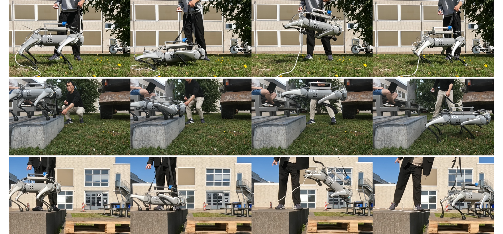
Figure 1: The Go1 jumps across outdoor environments. The robot jumps across grassland, jumps down onto grassland and across a gap onto a lower box.

In this work, we push robots to learn to jump on their own by combining curriculum learning with DRL, eliminating the reliability on prior motion references. By conditioning the policy on the desired landing location and orientation, our approach produces versatile jumping motions with just one single policy. Furthermore, by incorporating partial knowledge of the obstacles, the robot learns different manoeuvres adapted to complex real-world scenarios.

The main contributions are summarised as follows:

• We propose a curriculum-based DRL framework, which is capable of learning jumping motions without requiring motion capture data or a reference trajectory.

• We generalise across a wide range of jumps with a single policy, for both indoor and outdoor environments. With our method, the real robot can jump 90cm forward, which, to the best of our knowledge, is the longest distance achieved on quadrupeds of a similar size. It has been demonstrated that continuous jumping across grassland and robust jumping across uneven terrains can be achieved, in a zero-shot manner.

• We incorporate partial environmental information into the learning stage, which allows the robot to jump over more complex terrains.

In Section II, we introduce the existing RL-based jumping controllers. In Section III and Section IV, we separately present the curriculum design and DRL formulation. After extensively evaluating our method in Section V, we discuss our approach and directions for future work in Section VI.

II Related work

II-A Reinforcement learning for quadrupedal jumping

DRL is a promising solution for accomplishing jumping tasks by offloading the computational complexity to offline training. One approach to learning quadrupedal jumping is by learning from demonstrations, such as from trajectories generated through optimal control [9, 10], or hand-tuned reference motions [7, 8]. However, imitation-based methods have so far shown a limited generalisation capability beyond the imitation domain. Furthermore, many of the aforementioned works rely on learning a separate policy for each unique type of motion, rather than a common task- or goal-conditioned policy.

To reduce the dependency on a motion prior, [12] trained a high-level motion planning module to produce desired centre of mass (CoM) trajectories for small hops, conditioned on visual inputs and then tracked by a model-based controller. In [9], deviations to reference trajectories generated by a non-linear optimal trajectory [2] are learned, providing better generalisation to out-of-training domains. Recently, Vezzi et al. [13] proposed learning to jump by combining a first-stage evolution strategy with a second-stage DRL. Compared to [13], our approach is less complex by using proximal policy optimization (PPO) [14] for all curriculum stages, and is capable of executing jumps conditioned on the desired jumping length and orientation.

II-B Curriculum learning in dynamic quadrupedal locomotion

Curriculum learning (CL) [15] is a training framework which progressively provides more challenging data or tasks as the policy improves. As the name suggests, the idea behind the approach borrows from human education, where complex tasks are taught by breaking them into simpler parts.

In legged locomotion, CL has seen wide use, mainly in terms of terrain generation. Xie et al. [16] show how an adaptive curriculum can be used to learn stepping stone skills much more efficiently than other methods like uniform sampling. Similarly, other automatic curriculum learning methods have been proposed to vary environmental parameters based on the performance of the agents [5], rather than using a manually specified curriculum. On the rewards side, Hwangbo et al. [17] employ a curriculum which scales down certain rewards at the start. This design allows the policy to first learn how to locomote and only afterwards to be polished to satisfy the additional constraints and limits of the problem. In [18], vision-based parkour locomotion skills are learned through a well-designed terrain curriculum. To learn dynamic parkour skills, [19] adopt a two-stage curriculum, transitioning from soft to hard dynamic constraints in the second stage. Recently, [8] used multi-stage training to learn imitation-based vertical jumping, and then transferred that knowledge to forward jumping. While similar to our approach, however, there are a couple of significant differences - we do not require any reference trajectories, and we learn a single policy for versatile tasks.

III Curriculum design

Defining and constraining the behaviour of jumping across specific distances is challenging as it combines two distinct behaviours: that of "jumping" and that of reaching a desired spatial point. Furthermore, an easily learnable local optimum exists, where the robot could simply walk (or crawl) towards the target point without actually jumping. To avoid converging to such undesired behaviour we use curriculum learning to decompose the problem into several simpler sub-tasks.

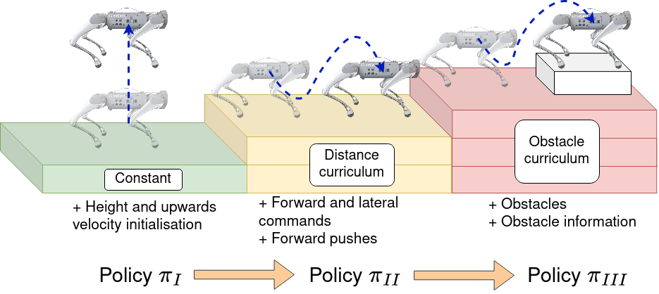
Figure 2: The curricula: jumping in place (left), long-distance jump (middle) and long-distance jump with obstacles (right). The latter two vary the jump distance/orientation and obstacle height, respectively.

In our approach, we adopt two types of curriculum - on a local difficulty level and on a task level, as can be seen in Fig. 2. The former involves progressively (and automatically) making the environment more complex as the agent succeeds. In particular, upon successful jumps, we increase the range of desired jumping distances and obstacle heights that we sample from. The task-level curriculum is, on the other hand, manually selected and consists of training the agent for a certain number of steps at a given task. After mastering the easier jumping skill, the policy is loaded onto the next task, which might be defined differently and contains a new set of rewards.

In the remainder , we describe each of these task-level and difficulty curricula in the progressive order of training.

III-A Stage I: Jumping in place

Vertical jumping without traversing a certain horizontal distance, i.e. jumping in place, is the basic component of agile jumping. However, the lack of reference results in a learning problem with sparse rewards, given that the agent needs to first learn certain behaviours (e.g., squatting down and then pushing hard against the ground to take off) before it can reach the reward-rich states, i.e. being high in the air. As the robot does not experience these jumping-specific rewards initially, it is prone to converging to a local optimum, such as standing in place, where small rewards are collected safely.

To avoid getting stuck in this local optimum behaviour, we adopt a modified form of the reference state initialisation (RSI) technique [20]. In imitation learning, RSI initialises the agent at random points of the reference trajectory, allowing the agent to explore such reward-rich states before it has learned the actions necessary to reach them. As we do not use a reference trajectory, we instead modify RSI to sample a random height and upward velocity from a predefined range.

III-B Stage II: Long-distance jump

Once the robot has converged to a jumping-in-place behaviour, we further train it to perform precise forward and diagonal jumps. The first part of the command vector $\mathbf{g}\in\mathcal{R}^{13}$ (see Fig. 4) in the observations specifies the desired landing point and orientation to create a goal-conditioned policy. Similarly to the jumping in place sub-task, we also adopt a curriculum-style sampling for desired landing points, where successful agents are progressed to more difficult environments where the desired jumping distance and landing yaw are sampled from a greater range.

III-C Stage III: Long-distance jump across obstacles

Finally, we introduce obstacles in the environment. Without loss of generality, we choose three classes of obstacles, including thin barrier-like objects, box-shaped obstacles and slopes. Depending on the desired landing pose, the obstacle location and the type, the agent needs to either jump onto or over it. While it is possible to learn a general behaviour that can accomplish this without any exteroception, such behaviour will be conservative, sub-optimal and potentially much less robust. With this in mind, we incorporate information about the distance to the centre of the obstacles and its general dimensions (length, width and height). In the real world, we manually specify these parameters.

Similarly to the previous stage, we start with obstacles of smaller height. Then, successful robots progress towards more challenging terrains whereas failing ones are demoted to easier environments. To ensure that the robot remembers the previously learned behaviour we also randomly send a certain percentage of robots to jump on flat ground, as in Stage II.

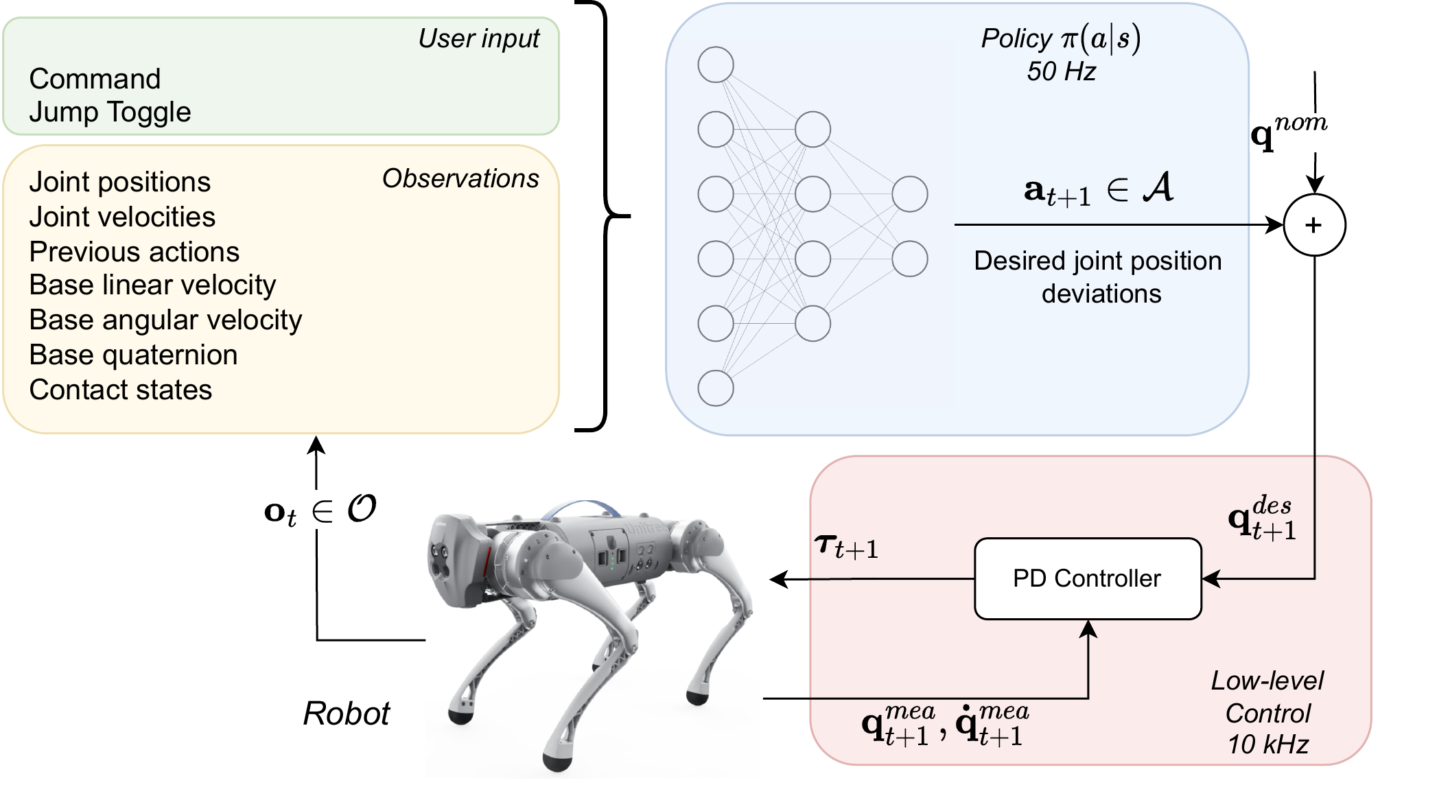
Figure 3: Control diagram of the system. The observations $\mathbf{o}_{t}$ include user command (in green) and a history of system states (in yellow). The policy is parameterised by a neural network (shown in blue). The output actions $\mathbf{a}_{t+1}$ are added to the nominal joint angles $\mathbf{q}^{nom}$. The desired joint angles are then tracked via a PD controller which computes torque commands.

IV DRL formulation

This section details the DLR formulation, as illustrated in Fig. 3. First, preliminaries are introduced. Then, we define the key components of goal-conditioned RL, including observations, actions and reward functions. Finally, we introduce our domain randomisation scheme to mitigate the sim2real gap.

IV-A Preliminaries

RL infers a policy $\pi(a_{t}|s_{t})$ of how to act by constantly interacting with the environment. The RL problem is typically formulated as a Markov decision process (MDP), where at each step the agent interacts with the environment by taking an action $\textbf{a}_{t}\in\mathcal{A}$. Subsequently, it receives the new states of the environment $\textbf{s}_{t+1}\in\mathcal{O}$ in the form of observation, and the associated reward $\mathcal{R}_{t}$ that it has earned. Based on the observed state $s_{t+1}$ and its policy $\pi(a_{t+1}|s_{t+1})$ the agent can then choose a new action $a_{t+1}$. In this way, the RL algorithm optimises behaviours that yield high rewards. In goal-conditioned RL, the action policy can also be conditioned on specific goals, i.e. $\pi(a_{t}|s_{t},g)$. Such a policy can be used to produce diverse behaviours depending on the specific command $g$, enabling the learning of multiple distinct behaviours under a single policy.

In this work, we formulate the following objective: finding a policy $\pi(a|s,g)$ which maximises the cumulative sum of rewards earned over the task duration. As often immediate rewards are more valuable than rewards in the distant future, a discount factor $\gamma\in(0,1]$ is commonly used. Mathematically, the full objective of maximising the sum of discounted rewards $J$, known as the return, can be written as:

$$\mathop{\arg\max\limits_{\mathbf{\pi}}}\quad J(\pi)=\mathbb{E}_{\tau\sim p^{\pi}(\tau)}[\sum_{t=0}^{T}\gamma^{t}R_{t}|s_{0}=s],$$ (1)

where $R_{t}$ is the immediate reward at time $t$ and $s_{0}$ is the initial state. The expectation of the return is taken over a trajectory $\tau$ sampled by following the policy.

IV-B Observation and action space

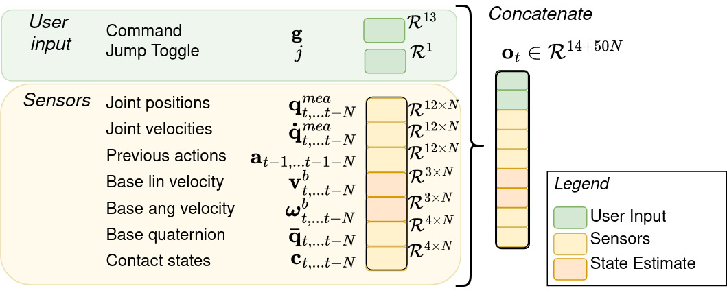
Figure 4: The definition of observations. The command $\mathbf{g}$ and jump toggle j are provided by the user, while the remaining observations are either directly read from the sensors, or estimated from sensor data.

Observation space: Using a memory of previous observations and actions allows the agent to implicitly reason about its own dynamics and the interaction with the environment [17, 5]. Here, we use a concatenated history of the last N steps as input to the policy. As illustrated in Fig. 4, the observation space consists of the historical base linear velocity $\mathbf{v}\in\mathbb{R}^{3\times N}$, base angular velocity $\bm{\omega}\in\mathbb{R}^{3\times N}$ (both in the base frame), joint position $\mathbf{q}\in\mathbb{R}^{12\times N}$, joint velocity $\mathbf{\dot{q}}\in\mathbb{R}^{12\times N}$, previous actions $\mathbf{a}_{-1}\in\mathbb{R}^{12\times N}$, the base orientation (as a quaternion) $\mathbf{\bar{q}}\in\mathbb{R}^{4\times N}$ and the foot contact states $\mathbf{c}\in\mathbb{R}^{4\times N}$.

Note that our policy is also conditioned on the command $\mathbf{g}\in\mathbb{R}^{13}$ and jump toggle $j\in\{0,1\}$, see the green block in Fig. 4. As illustrated in Fig. 5, the command $\mathbf{g}\in[\Delta\mathbf{p}_{des},\Delta\mathbf{\bar{q}}_{des},\mathbf{p}_{obs},\mathbf{dim}_{obs}]$ contains the desired landing position ($\Delta\mathbf{p}_{des}\in\mathbb{R}^{3}$), desired landing orientation ($\Delta\mathbf{\bar{q}}_{des}\in\mathbb{R}^{4}$), the centre of the obstacle ($\mathbf{p}_{obs}\in\mathbb{R}^{3}$ if present), and its dimensions ($\mathbf{dim}_{obs}\in\mathbb{R}^{3}$ including height, width, length). Due to the lack of long-term memory in the feed-forward neural network, we use the jump toggle $j$ to indicate whether the robot has already jumped, similar to [20]. However, in our case, the jump toggle also serves as a control switch, where the robot remains standing until its value is changed.

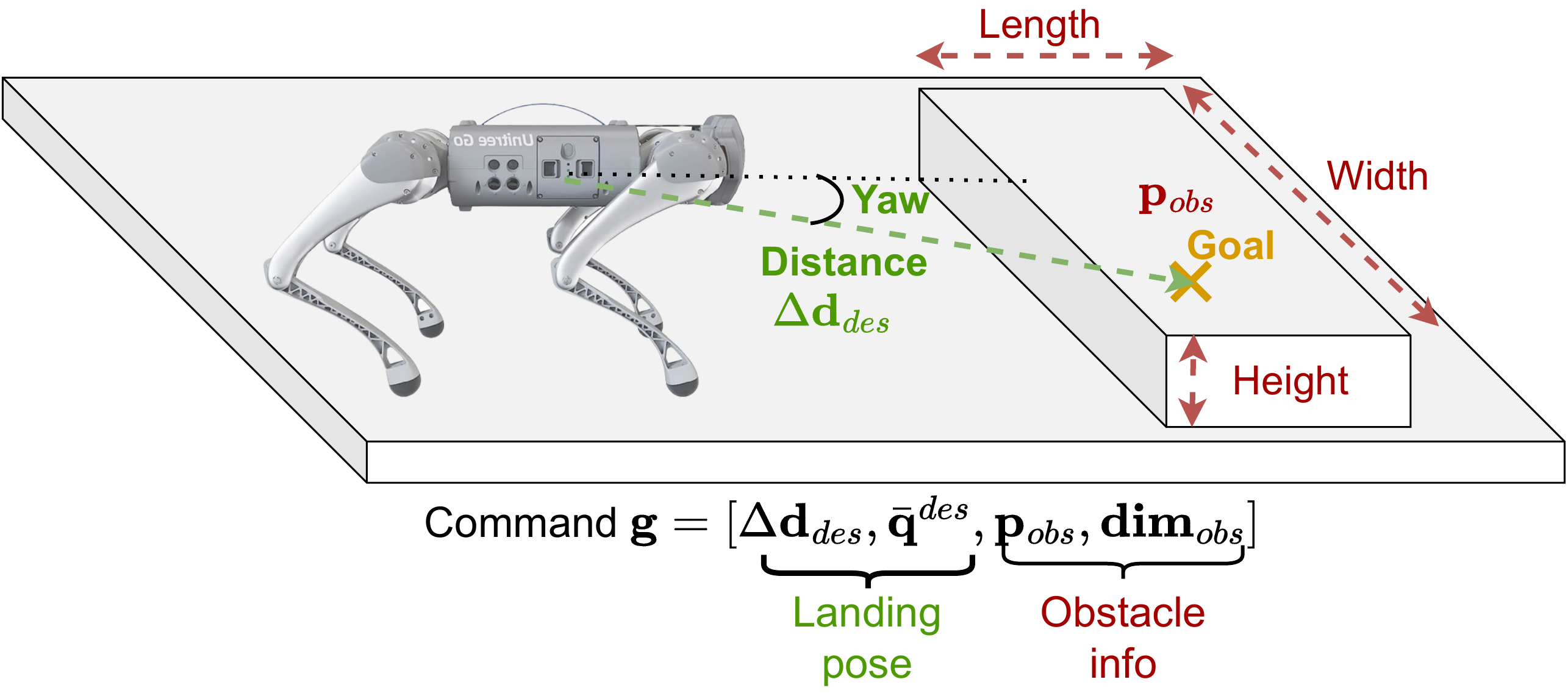
Figure 5: The command vector $\mathbf{g}$ for a forward jump onto an obstacle. In the first two training stages ($\pi_{I}$ and $\pi_{II}$) where no obstacles are considered, the information of the obstacle is set to zero.

Action space: Our policy generates the twelve actuated joint angles ($\mathbf{q}^{des}\in\mathbb{R}^{12}$) for jumping control. Particularly, we learn the deviations from the nominal joint positions $\mathbf{q}^{nom}\in\mathbb{R}^{12}$. To smooth the output actions, we used an exponential moving average (EMA) low-pass filter with a cut-off frequency of 5 Hz. The filtered actions are then scaled and added to $\mathbf{q}^{nom}$ to generate $\mathbf{q}^{des}$ for the motor servos, i.e. $\mathbf{q}^{des}=\mathbf{a}+\mathbf{q}^{nom}$. A PD feedback controller then produces the desired torque at a higher frequency, as shown in Fig. 3. To guarantee safety, we clip $\mathbf{q}^{des}$ within the feasibility range when the real joint angles approach the limits.

IV-C Rewards

TABLE I: Rewards definition. The light orange colour indicates task-based rewards, while the light purple shade describes regularisation rewards.

Name	Type	Stance	Flight	Landing
Landing position	Single	0	0	$w_{p}(e(\sum|\mathbf{p}_{land}-\mathbf{p}_{des}|^{2}))$
Landing orientation	Single	0	0	$w_{ori}(e(|log(\mathbf{\bar{q}}_{land}^{-1}*\mathbf{\bar{q}}_{des}|^{2}))$
Max height	Single	0	0	$w_{h}(e(|h_{max}-0.9|^{2}))$
Jumping	Single	0	0	$w_{jump}$
Base Position	Continuous	$w_{p_{z},sq}(e(|p_{z}-0.20|^{2})$	$w_{p_{z},fl}(e(|p_{z}-0.7|^{2})$	$w_{p.l}(e(\sum|\mathbf{p}-\mathbf{p}_{land}|^{2}))$
Orientation Tracking	Continuous	$w_{ori,st}(e(|log(\mathbf{\bar{q}}_{base}^{-1}*\mathbf{\bar{q}}_{des}|^{2}))$	0	$w_{ori,l}(e(|log(\mathbf{\bar{q}}_{base}^{-1}*\mathbf{\bar{q}}_{des}|^{2}))$
Base lin. velocity	Continuous	0	$w_{\mathbf{v}_{x,y}}(e(\sum|\mathbf{v}_{x,y}-\mathbf{v}_{des}|^{2})$	0
Base ang. velocity	Continuous	0	$w_{\bm{\omega}}(e(\sum|\bm{\omega}-\bm{\omega}_{des}|^{2})$	$0.1w_{\bm{\omega}}(e(\sum|\bm{\omega}-\mathbf{0}|^{2})$
Feet clearance	Continuous	0	$w_{feet}e(|p_{feet}-p_{feet}^{0}+[0.0,0.0,-0.15]|^{2})$	0
Symmetry	Continuous	$w_{sym}(\sum_{joint}|\mathbf{q}_{left}-\mathbf{q}_{right}|^{2})$
Nominal pose	Continuous	$w_{q}(e(\sum_{joint}|\mathbf{q}_{j}-\mathbf{q}_{j,nom}|^{2})$	0.1$w_{q}(e(\sum_{joint}|\mathbf{q}_{j}-\mathbf{q}_{j,nom}|^{2})$	$w_{q}(e(\sum_{joint}|\mathbf{q}_{j}-\mathbf{q}_{j,nom}|^{2})$
Energy	Continuous	$w_{energy}(\bm{\tau}^{T}\mathbf{\dot{q}})$
Base acceleration	Continuous	$w_{acc}|\mathbf{\dot{v}}|^{2}$
Contact change	Continuous	$w_{c}\sum_{feet}(c_{foot}(t)-c_{foot}(t-1))$
Contact forces	Continuous	$w_{F_{c}}\sum_{i=0}^{n_{f}}|F_{i}-\bar{F}|$
Action rate	Continuous	$w_{a}\sum_{joint}|\mathbf{a}(t)-\mathbf{a}(t-1)|^{2}$
Joint acceleration	Continuous	$w_{\ddot{q}}\sum_{joint}|\mathbf{\ddot{q}}_{j}|^{2}$
Joint limits	Continuous	$w_{q_{lim}}\sum_{joint}|\mathbf{q}_{j}-\mathbf{q}_{j,lim}|^{2}$

Ideally, we expect the agent to accomplish the task while maximising the rewards it receives. However, poor choice of reward scaling could lead the agent to converge to the local minima, e.g., standing behaviour without jumping, where only certain penalties like energy cost and joint acceleration are minimised. To avoid this, instead of naively summing them, we multiply the positive component of the reward by the exponent of the negative component, i.e. $r_{total}=r^{+}e(|r^{-}|^{2})$. This allows the agent to always receive a strictly positive reward, scaled down by the amount of penalties, which improves the learning stability.

As listed in Table I, three phases are used to describe when each reward is given. In particular, ‘stance’ indicates that the robot has been given a command to jump but is still on the ground. Then, ‘flight’ is triggered when the robot is in mid-air and has no contact with the ground. Finally, the ‘landing’ begins upon landing and lasts until the end of the episode. In each phase, task-based rewards (in orange) and regularisation rewards (in violet) are considered. On the other hand, the rewards items can be divided into Single type and Continuous type, where the former is given once per episode (typically at the end), and the latter is given once per each simulation step that satisfies the conditions.

Task rewards: First, sparse rewards are introduced to encourage the general behaviour for accomplishing the desired jumping task, including those of detecting contact (‘landing’) after several steps of no contact (‘flight’), the maximum height the agent reached, and whether it has landed at the desired position with the desired orientation. These rewards are only given once at the end of the episode, marked by ‘Single’ in Table I. In addition, continuous task-related objectives are also defined to simplify the exploration, including

• Tracking the desired linear velocity ($\mathbf{v}^{b}_{x,y,des}$) and yaw angular velocity while in flight, and tracking zero angular velocity after landing.

• Squatting down to a height of 0.2m while on the ground and tracking a certain height in the air.

• Maintaining a constant base position and tracking the desired orientation after landing.

Notably, in order to ensure enough clearance when jumping forward and over obstacles, we introduce a foot clearance reward that tracks the nominal foot position (i.e. at the nominal joint angles $q^{nom}$) on the xy-plane, and simultaneously, minimises the z-distance between each foot and the centre of mass. This objective encourages the robot to tuck its legs in close to its body while in the air.

Regularisation rewards: As we do not imprint any reference motions onto the agent, auxiliary regularisation rewards are needed to achieve smooth, feasible and safe behaviour. Specifically, we penalise the action rate, together with any violations of predefined soft limits for the joint position. Besides, the instantaneous energy power, computed as the dot product between actuator torque and joint velocity, is penalised for generating an energy-efficient motion. Considering that various quadrupedal jumps seen in nature exhibit high left- and right-side symmetry, we drive the robot towards maintaining this symmetry with an additional reward. Finally, we noticed that the robot often stomped its feet rapidly during the squat-down stage in the training process. To eliminate this unnecessary behaviour, we add a small reward for maintaining the same contact states for each foot between simulation steps.

Termination: We terminate each episode when the following events occur:

• Collision between body links and the environment.

• Base height lower than 0.12 m.

• Orientation error larger than 3.0 rad.

• Landing position error bigger than 0.15 m.

IV-D Domain randomisation

TABLE II: Randomised variables and their ranges.

Name	Randomisation range
Ground friction	[0.01, 3.0]
Ground restitution	[0.0, 0.4]
Additional payload	[-1.0, 3.0] $\mathrm{kg}$
Link mass factor	[0.7,1.3] x
Centre of mass displacement	[-0.1, 0.1] $\mathrm{m}$
Episodic Latency	[0.0, 40.0] $\mathrm{ms}$
Extra per-step latency	[-5.0, 5.0] $\mathrm{ms}$
Motor Strength factor	[0.9, 1.1] x
Joint offsets	[-0.02, 0.02] $\mathrm{rad}$
PD Gains factor	[0.9, 1.1] x
Joint friction	[0.0, 0.04]
Joint damping	[0.0, 0.01] $\mathrm{N}\text{\,}\mathrm{m}\text{\,}\mathrm{s}\text{\,}{\mathrm{rad}}^{-1}$

To bridge the gap between simulation and real-world scenarios, we implement zero-shot domain randomisation. The ground friction, restitution, and link mass are sampled at random at the start of every episode. In addition, we add a random offset to the joint encoder values, randomise proportional and derivative gains of the PD controller and randomise the strength of the motors for every episode. The range of each randomized variable is listed in Table II.

For hardware control, unmodelled communication delays and latencies strongly weaken the performance of learning-based policies. To tackle this issue, at the beginning of each episode, we sample a latency value from the range of $l\in[0,50]$ ms. Then, at each step, we add a small random value to reflect the effect of stochastic communication delays.

V Experimental validation

In this section, we first validate the policy trained on the first two curriculum stages (i.e. policy $\pi_{II}$, shown in Fig. 2), through various experiments - forward and diagonal jumps, continuous jumps, and robust jumping in the presence of environmental disturbances and uneven terrains. Then, we validate the policy after the final training stage (policy $\pi_{III}$) when jumping onto and over obstacles.

V-A Training setup

The implementation is based on the open-source Gym environment provided by ETH Zurich [4]. Particularly, we use 4096 agents and 24 environmental steps per agent per update step. For the vertical jump, we train for 3k iterations, while for the forward jump without and with obstacles we train for 10k steps each. The actor policy and the critic are parameterised by a shared MLP with 3 hidden layers of dimensions $[256,128,64]$, with exponential linear unit (ELU) activations after each layer. Using a single RTX 3090 GPU, the three highly parallelised training stages took approximately 1.4 hours, 4.1 hours and 4.8 hours, respectively.

The policy operates at a frequency of 50 Hz, and the simulation runs at 200 Hz. We performed all of the experiments on the Unitree Go1. During the hardware validations, we use a constant joint friction value of 0.04, joint damping of 0.01 Nm s rad^-1 and a constant latency of 30 ms.

V-B Versatile jumping on flat ground

V-B1 Forward jumping

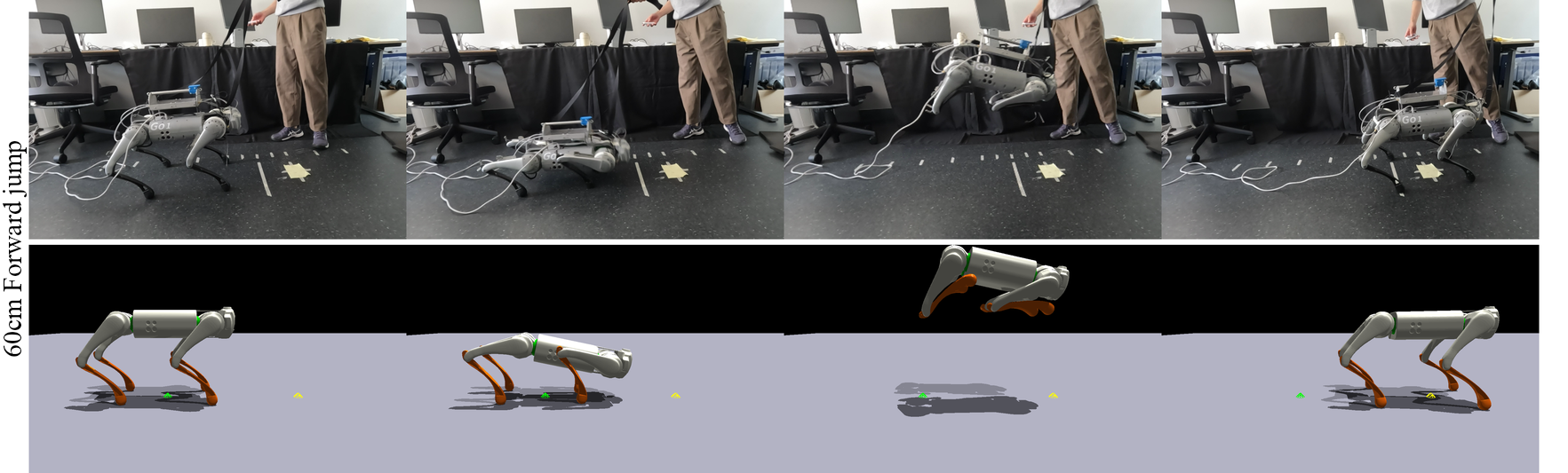
Figure 6: Real world (top) and simulation (bottom) execution of a forward jump. The yellow marker indicates the desired 60cm jumping distance.

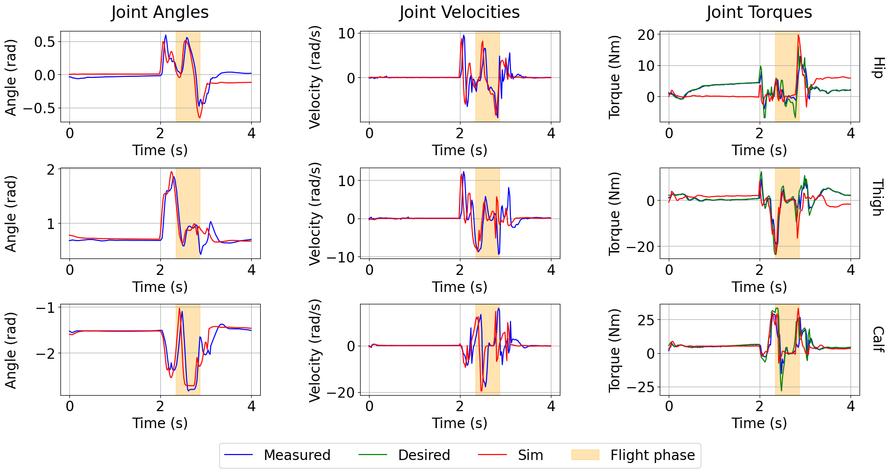
(a) Joint angles, velocities and torques for the front right (FR) leg during the 60cm forward jump. The flight phase for the hardware experiment is indicated by the yellow-shaded region.

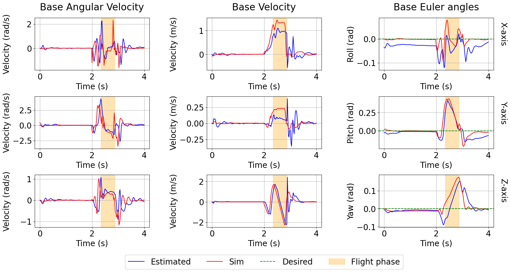
(b) Base angular and linear velocity during the 60cm forward jump. The flight phase for the hardware test is indicated in light yellow.

Figure 7: Hardware and simulation quantitative results for the 60cm forward jump.

First, we evaluate the policy on a variety of forward jumps. Fig. 6 compares hardware and simulation motions of a 60cm forward jump while Fig. 7 presents the quantitative results. As can be seen, the real-world behaviour closely matches the simulated prediction. One noticeable deviation is in the peak torques at take-off - where the measured torques deviate from both the desired torques (computed by the PD control law using the desired joint angles) and the simulation torques. Besides, larger joint angles for the hip and thigh are measured upon landing in real-world tests, likely due to poor impact modelling in the simulation. Finally, the Euler angles show a slight variation between simulation and hardware. We believe that this mismatch is mainly due to the motor modelling inaccuracies, coupled with the weight of the additional mass on top of the robot, shifting its centre of mass. Despite these state deviations, the jumping distance is well-tracked, and the base velocity matches the expected behaviour, showing a good sim2real adaptation.

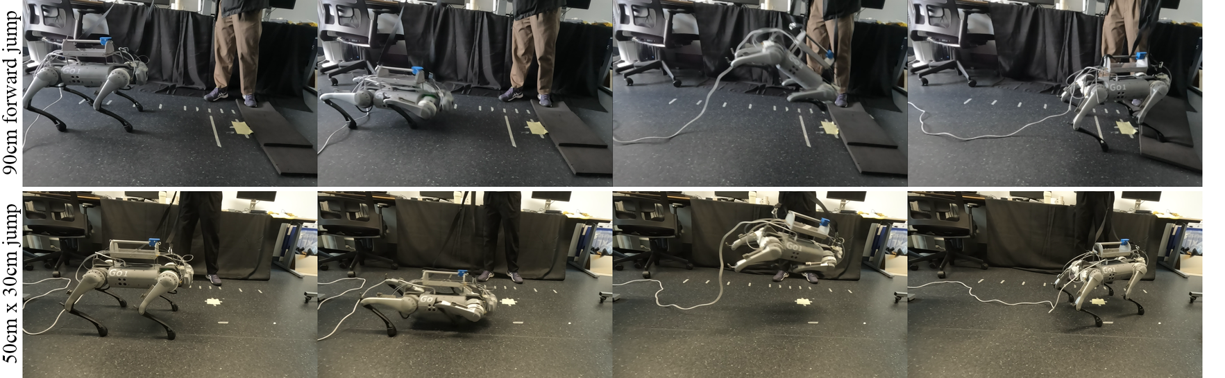
Figure 8: Hardware results for a 90cm forward jump (top) and a 50cm $\times$ 30cm diagonal jump with desired yaw of $30\degree$ (bottom).

We then tested the maximum distance it could jump across. Fig. 8(top) illustrates a 90 cm forward jump, with the target landing point shown by the yellow marker. Despite slipping on the soft pads as it lands, the robot recovers quickly, demonstrating its robustness against uncertainties. To the best of our knowledge, this is the largest jumping distance achieved by robots of similar size and similar actuators (see Table III).

TABLE III: Maximal jump length comparison with state-of-the-art.

Method	[21]	[12]	[22]	[23]	[18]	Ours
Jump length [m]	0.2	0.26	0.5	0.6	0.8	0.9

V-B2 Diagonal jumping

Fig. 8(bottom) shows a diagonal jump of 50 cm x 30 cm with a desired yaw of $30\degree$. Both the landing position and yaw are tracked accurately.

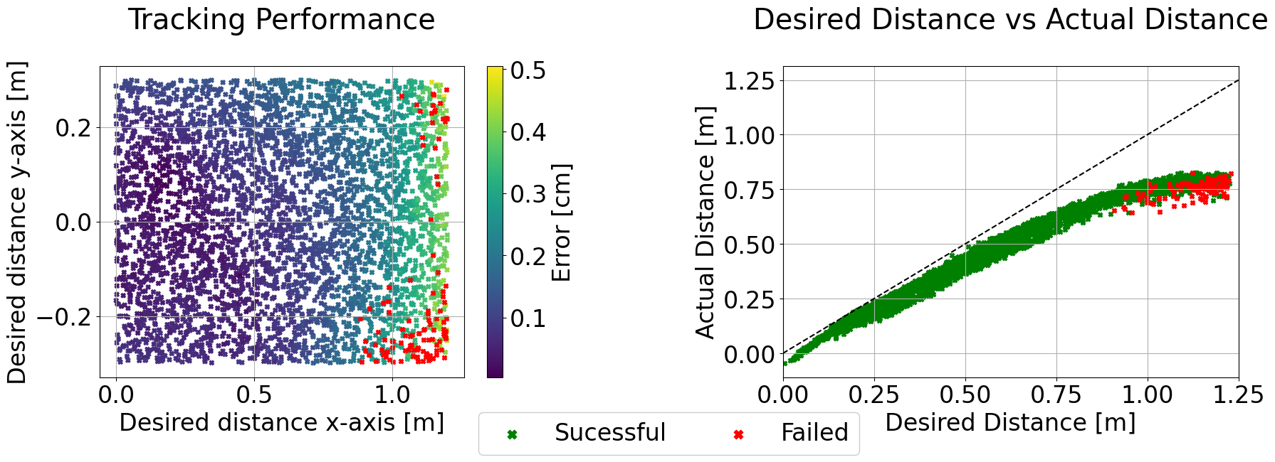
Figure 9: Tracking performance as a function of the desired X- and Y-axis jumping distances, with the error (in cm) shown by the colour gradient (left); and the tracking performance in terms of overall desired vs actual jumping distance (right). The environments that have been terminated (due to any non-foot collisions) are shown in red, and the black $45\degree$ dashed line indicates the ideal tracking performance. Data is gathered from 8000 trials across the whole jumping range $x\in[0,1.2],y\in[-0.3,0.3]$.

Furthermore, we evaluated the policy across the whole jumping range in simulation, of which the success rate and tracking metrics are presented in Fig. 9. As can be seen from the left plot, the tracking error is lowest for narrow jumps of forward distance up to 50 cm. As both the longitudinal and lateral distances increase, so does the final landing error. Interestingly, the majority of failed environments asymmetrically occur in the lower right corner of the plot. The right plot in Fig. 9 shows the same data but grouped by total desired distance vs actual achieved distance. We found that the data closely follow the $45\degree$ line (i.e. ideal performance) for the smaller jumps with the gradient slowly decreasing after 50 cm.

V-C Jumping onto/across rough terrain

We here evaluate how well the policy performs in the presence of environmental disturbances, despite not being trained on uneven or rough ground. In this section, we ran several experiments, including jumping with obstacles surrounding the robot, blindly jumping from and onto a box, and jumping from asphalt onto a soft grassy terrain. As shown by the top two time-lapses in Fig. 10, the policy enables robust jumping onto both soft and stiff objects that could (and did) slip under the feet of the robot. The third row demonstrates that the robot could jump from hard asphalt onto soft grass, despite training on flat ground only.

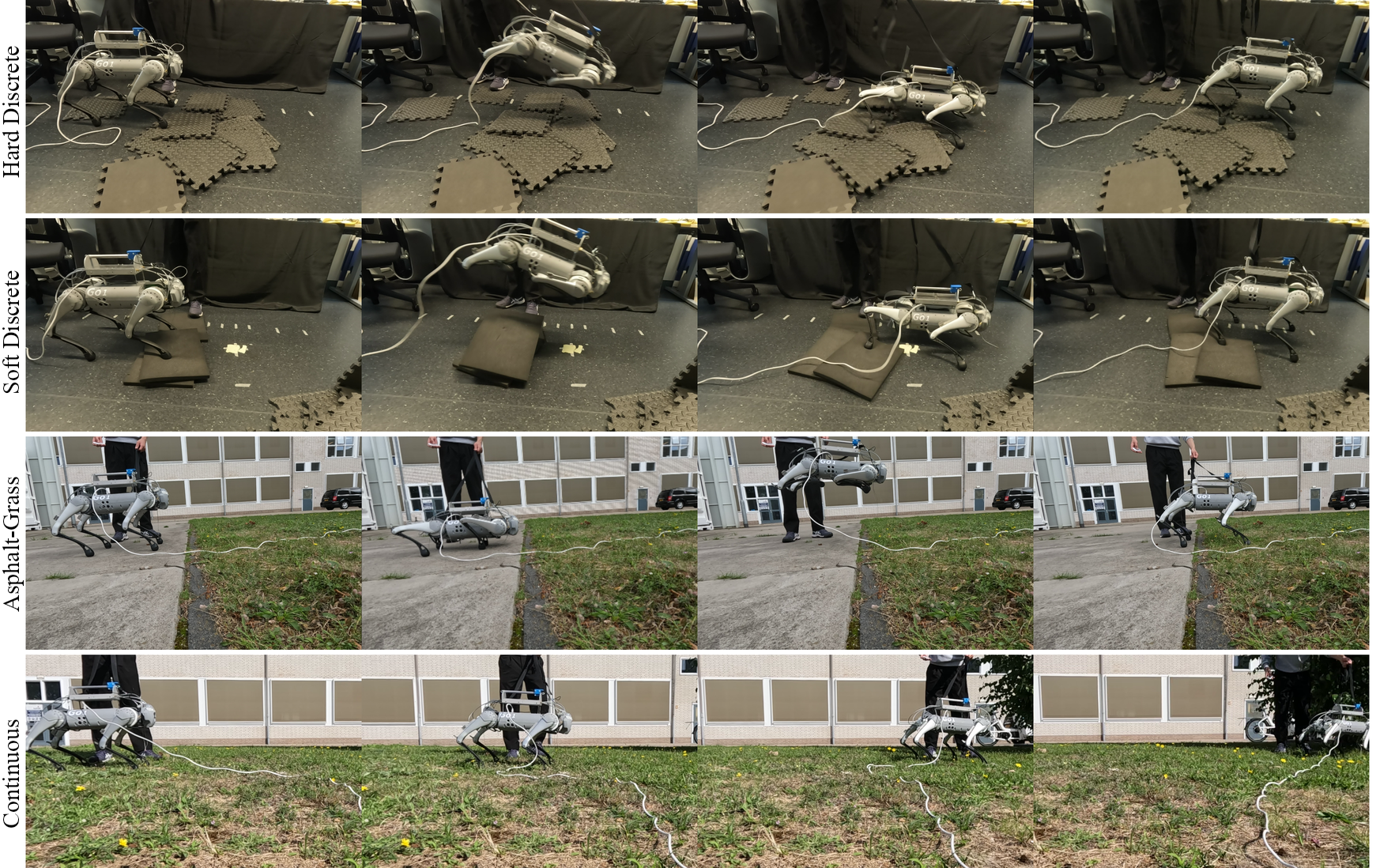
Figure 10: Several experiments showcasing the robustness of the policy $\pi_{II}$ to variations in the terrain: jumping across discrete hard and soft objects (rows 1 and 2), asphalt-to-grass jump (row 3), nine consecutive jump on grass (row 4).

Next, we tested the policy on a continuous jumping task, where a new command of a 40cm forward jump is given following each jump without resetting the robot states. As seen in the fourth row of Fig. 10, the policy is robust enough to execute a jump from a variety of different initial states. Despite the fact that the soft ground causes some hip angle deviation upon landing, the robot was able to execute at least nine consecutive jumps.

V-D Forward jumping with obstacles

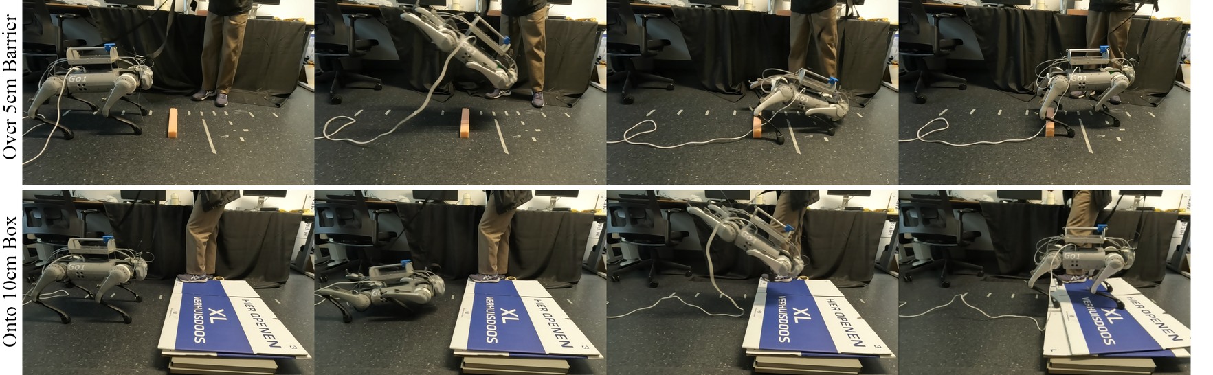
Figure 11: Jumping over a 5cm tall, 5cm wide obstacle (top row) and jumping onto a 10cm tall box (bottom).

To further demonstrate the versatility, we tested forward jumping with obstacles, using policy $\pi_{III}$. To be brief, only two scenarios are presented here, including jumping over a 5 cm tall thin obstacle and landing on a 10 cm box. In the first task, the robot had to jump across 80 cm to avoid collision. As seen in the top row of Fig. 11, the robot succeeded in jumping over the barrier and landed successfully. In the second case, the robot needed to leap over 70 cm while maintaining a large height. As a result, better performance was observed, considering that a shorter forward distance enabled the robot to achieve a larger height throughout the flight.

V-E Ablation study

To better understand the effect of our curriculum, we compared our approach to several baselines in Fig. 12:

• No RSI: Training Stage I without RSI, i.e. no height and upward velocity initialisation,

• No curriculum: Directly training Stage II without pre-training Stage I, but with RSI height and velocity initialisation. For fairness, we train this baseline for an additional 3k steps,

• No curriculum and no RSI: Same as above, but without any RSI.

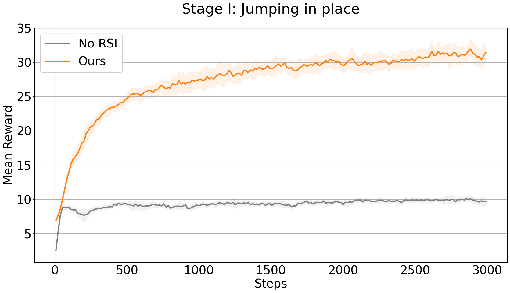
(a)

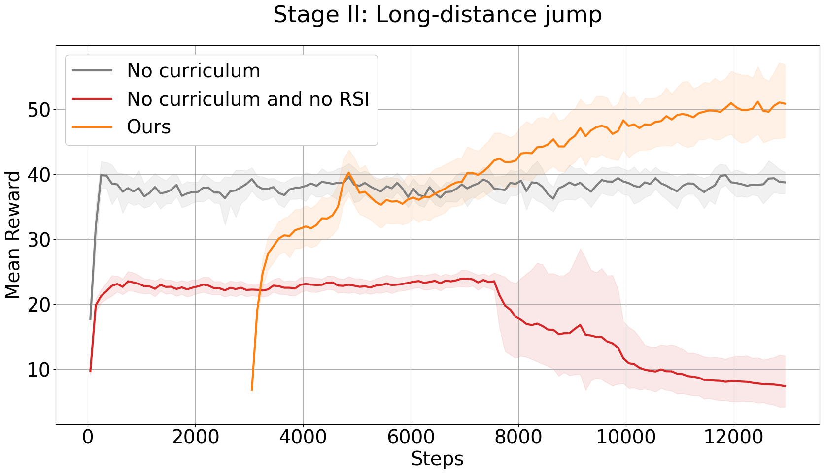
(b)

Figure 12: Mean reward throughout training for the (a) Stage I: Jumping in place, and (b) Stage II: Long-distance jump tasks.

As can be seen from Fig. 12a, the RSI is required for learning the jumping-in-place task. Without it, the agent converges to a local optimum and fails to complete the task. Despite the overall high reward, it can be seen in Fig. 12b that directly training the long-distance jump also results in an early convergence to a standing behaviour, which highlights the need for our curriculum strategy.

VI Discussion and conclusion

In this work, we present a curriculum-based end-to-end deep reinforcement learning approach, capable of learning a variety of precise short- and long-distance jumps, while also reaching the desired yaw upon landing. Unlike many existing methods, we have achieved this through a single policy, without the need for reference trajectories and additional imitation rewards. Furthermore, through domain randomisation, we successfully deployed the policy onto the real system and closely matched the expected behaviour from the simulation. The system was robust to the noisy sensor data, especially the foot contact sensors and the velocity state estimates. The jumps exhibited high accuracy, both in simulation and on the hardware, in terms of tracking the desired landing position and orientation. Furthermore, our policy achieved a 90 cm forward jump on the Unitree Go1 robot, a distance greater than those reported by other model- and learning-based controllers. We demonstrated additional outdoor tests, where the robot successfully performed nine consecutive jumps on soft grass, without previously encountering such environments in its training. In addition, we showed that simulating obstacles throughout training and conditioning the policy on their properties can enhance the mobility of the robot, allowing it to safely leap over or land on objects of up to 10cm.

When executing a long-distance jump, real animals exhibit a four-legged contact phase, followed by an upward pitch and pure rear-leg contact at take-off. During landing a mirrored behaviour is observed - the body is pitching downwards and contact is first gained with the front legs. Previous model-based control works [1, 2] have manually incorporated this contact schedule into their optimisers. It would be interesting to investigate how such behaviour can be learned through DRL without supplying a reference trajectory, and validate its benefits compared to the style of jumping exhibited here.

References

- [1] Quan Nguyen et al. “Optimized Jumping on the MIT Cheetah 3 Robot” In International Conference on Robotics and Automation, 2019, pp. 7448–7454
- [2] Chuong Nguyen and Quan Nguyen “Contact-timing and trajectory optimization for 3d jumping on quadruped robots” In IEEE/RSJ International Conference on Intelligent Robots and Systems, 2022, pp. 11994–11999
- [3] Jiatao Ding et al. “Robust Jumping with an Articulated Soft Quadruped via Trajectory Optimization and Iterative Learning” In IEEE Robotics and Automation Letters 9.1 IEEE, 2023, pp. 255–262
- [4] Nikita Rudin, David Hoeller, Philipp Reist and Marco Hutter “Learning to Walk in Minutes Using Massively Parallel Deep Reinforcement Learning” In Conference on Robot Learning, 2022, pp. 91–100
- [5] Joonho Lee et al. “Learning quadrupedal locomotion over challenging terrain” In Science Robotics 5.47, 2020, pp. eabc5986
- [6] Takahiro Miki et al. “Learning robust perceptive locomotion for quadrupedal robots in the wild” In Science Robotics 7.62, 2022, pp. eabk2822
- [7] Chenhao Li et al. “Learning Agile Skills via Adversarial Imitation of Rough Partial Demonstrations” In Conference on Robot Learning 205, 2022, pp. 342–352
- [8] Zhongyu Li et al. “Robust and Versatile Bipedal Jumping Control through Multi-Task Reinforcement Learning” In CoRR abs/2302.09450, 2023
- [9] Guillaume Bellegarda and Quan Nguyen “Robust Quadruped Jumping via Deep Reinforcement Learning” In CoRR abs/2011.07089, 2023
- [10] Yuni Fuchioka, Zhaoming Xie and Michiel Panne “OPT-Mimic: Imitation of Optimized Trajectories for Dynamic Quadruped Behaviors” In International Conference on Robotics and Automation, 2023, pp. 5092–5098
- [11] Fangzhou Yu et al. “Dynamic Bipedal Maneuvers through Sim-to-Real Reinforcement Learning” In CoRR abs/2207.07835, 2022
- [12] Gabriel B. Margolis et al. “Learning to Jump from Pixels” In Conference on Robot Learning 164 PMLR, 2021, pp. 1025–1034
- [13] Francecso Vezzi et al. “Two-Stage Learning of Highly Dynamic Motions with Rigid and Articulated Soft Quadrupeds” arXiv, 2023 arXiv:2309.09682
- [14] John Schulman et al. “Proximal policy optimization algorithms” In arXiv preprint arXiv:1707.06347, 2017
- [15] Yoshua Bengio, Jérôme Louradour, Ronan Collobert and Jason Weston “Curriculum learning” In International Conference on Machine Learning, 2009, pp. 41–48
- [16] Zhaoming Xie, Hung Yu Ling, Nam Hee Kim and Michiel Panne “ALLSTEPS: Curriculum-driven Learning of Stepping Stone Skills” In Computer Graphics Forum 39.8, 2020, pp. 213–224
- [17] Jemin Hwangbo et al. “Learning agile and dynamic motor skills for legged robots” In Science Robotics 4.26, 2019, pp. eaau5872
- [18] Xuxin Cheng, Kexin Shi, Ananye Agarwal and Deepak Pathak “Extreme Parkour with Legged Robots” arXiv, 2023 arXiv:2309.14341
- [19] Ziwen Zhuang et al. “Robot Parkour Learning” arXiv, 2023 arXiv:2309.05665
- [20] Xue Bin Peng, Pieter Abbeel, Sergey Levine and Michiel Panne “DeepMimic: example-guided deep reinforcement learning of physics-based character skills” In ACM Transactions on Graphics 37.4, 2018, pp. 143:1–143:14
- [21] Laura M. Smith et al. “Learning and Adapting Agile Locomotion Skills by Transferring Experience” In Robotics: Science and Systems XIX, 2023
- [22] Ken Caluwaerts et al. “Barkour: Benchmarking Animal-level Agility with Quadruped Robots”, 2023
- [23] Yuxiang Yang et al. “Continuous Versatile Jumping Using Learned Action Residuals” In Annual Learning for Dynamics and Control Conference, 2023, pp. 770–782