Condensation mass sink and intensification of tropical storms

Abstract

Intensification of tropical storms measured as the central pressure tendency represents a subtle imbalance, of the order of $10^{-3}$, between the inflow and outflow of air in the storm core. Factors driving this imbalance, especially in cases of rapid intensification, remain elusive. Here, using an analysis of intensification rates and precipitation in North Atlantic cyclones, it is shown that the storms on average deepen at a rate with which maximum local precipitation removes mass from the atmospheric column. Means for lifetime maximum intensification rate and maximum concurrent precipitation (multiplied by the acceleration of gravity) are, respectively, $23$ and $17$ hPa day^-1. This equivalence is not limited to average values: both intensification rates and precipitation have the same dependence on the inverse radius of maximum wind. It is further shown using a numerical model that with the mass sink switched off, storms driven by sensible and latent heat alone either do not develop at all or develop significantly more slowly reaching lower maximum intensities. It is discussed that the conclusions of previous studies about the relative insignificance of the mass sink arose from a long-standing misinterpretation of mass nonconservation assessments for assesments of the actual impact of the mass sink on storm dynamics. Condensation mass sink provides for a fundamental positive feedback between surface pressure and vertical velocity that was earlier shown to be instrumental in analytical descriptions of storm intensification. This feedback allows the storm circulation to get more compact during intensification in contrast to modeled heat-driven storms that increase their radius of maximum wind as they intensify. These findings indicate that the condensation mass sink is a dominant process governing the dynamics of tropical storms.

1 Introduction

Rapid intensification of tropical storms defies reliable forecasting, threatens human lives and property, and largely remains enigmatic. Holliday and Thompson (1979) analyzed maximum deepening rates (the largest daily drop in central surface pressure during the storm’s lifetime) for $305$ North Pacific typhoons and found a median of $24$ hPa day^-1. The $75$th percentile, $42$ hPa day^-1, was defined as the rapid intensification threshold. For North Atlantic cyclones, the threshold was defined in terms of daily velocity increment (Kaplan and DeMaria, 2003). Defining intensification rate via central pressure tendency has the merit of emphasizing that a low surface pressure is necessary to intensify the storm’s circulation (Rodgers and Adler, 1981).

Since the atmosphere is approximately hydrostatic, in order for the surface pressure to drop, the mass of the atmospheric column must decrease. From this perspective, rapid intensification represents a remarkably subtle imbalance between the inflow $F_{\rm in}$ and outflow $F_{\rm out}$ of air in the storm core. Consider an axisymmetric cyclone with radial velocity $u_{\rm in}$ in the vicinity of the radius of maximum wind $r_{m}$ within the boundary layer of depth $h_{\rm in}$. How fast does the inflow $F_{\rm in}=2\rho_{s}u_{\rm in}h_{\rm in}/r_{m}$ (see Appendix A) recycle matter within the cylinder of radius $r_{m}$? The turnover time is given by

$$\tau_{F}=\frac{\rho_{s}H}{F_{\rm in}}=\frac{r_{m}H}{2u_{\rm in}h_{\rm in}},$$ (1)

where $\rho_{s}$ is air density at the surface, $H$ is the exponential height of air density, and $\rho_{s}H$ (kg m^-2) is the total air mass of the atmospheric column. For characteristic values $u_{\rm in}=20$ m s^-1, $r_{m}=40$ km, $h_{\rm in}=1$ km, $H\sim 10$ km, and $\rho_{s}=1$ kg m^-3, we obtain $\tau_{F}=10^{4}$ s $\simeq 2.8$ hours.

Meanwhile with a typical maximum intensification rate of the order of $20$ hPa day^-1, the entire column with surface pressure $\leavevmode\nobreak\ 10^{3}$ hPa would have been depleted in $\tau_{P}=50$ day $\simeq 4\times 10^{6}$ s. This means that, even during maximum intensification, the inflow and outflow of air into and from the hurricane core must coincide with each other with a high precision of a fraction of percent, $\tau_{F}/\tau_{P}=0.002$. The outflow and inflow are apparently tightly “slaved” to one another (Smith and Montgomery, 2016a).

What determines this subtle imbalance between the outflow and inflow of atmospheric air that dictates how fast the storm intensifies? Is there a process inherent to tropical cyclones that would be characterized by a relevant magnitude? Yes, there is such a process. Tropical cyclones are well known for their extreme precipitation rates. In the North Atlantic hurricanes precipitation within $100$ km from the center reaches $P=200$ kg m^-2 day^-1 exceeding the local long-term climatological mean by a factor of forty (Lonfat et al., 2004; Makarieva et al., 2017a; Tu et al., 2021). If matter is removed from a hydrostatic air column at this rate, surface pressure will drop by $gP\simeq 20$ hPa day^-1 ($g$ is the acceleration of gravity). This is close to the characteristic maximum intensification rate as established by Holliday and Thompson (1979). In other words, during maximum intensification the mean surface pressure tendency in the storm’s core of radius $r$ is of the order of local precipitation times $g$ and can be written as (see Appendix A):

$$\frac{1}{g}\frac{\partial p}{\partial t}=F_{\rm in}-F_{\rm out}-P\sim-P.$$ (2)

Despite it being the leading term in the mass budget for the storm core, the condensation mass sink appears to have been completely excluded from theoretical investigations of storm intensification. Even when diagnosing the central pressure tendency from the continuity equation, the mass sink has recently been set to zero (see Eq. (1) and subsequent derivations of Sparks and Toumi, 2022a). This situation appears to have been grounded in a long-standing confusion, which we here intend to clarify.

Lackmann and Yablonsky (2004) estimated that precipitation in Hurricane Lili (2002) was sufficient to account for the storm’s intensification rate and used that as a motivation to investigate the potentially significant impact of the precipitation mass sink on storm intensity. Since water vapor is a minor atmospheric constituent, in the continuity (mass conservation) equation the mass sink is a minor term that is often neglected. Lackmann and Yablonsky (2004) restored the mass sink in the system of equations solved by a numerical model for Hurricane Lili (2002) and compared the output of thus modified model with the control (with no mass sink in the continuity equation).

The authors concluded that the mass sink was not negligible but not dominant either (increasing the maximum drop of surface air pressure by a few hectopascals and maximum intensity by a few meters per second, Table 1). However, this conclusion cannot be considered satisfactory for a reason that, surprisingly, has never been discussed: the mass sink was present in the control simulation as well. Lackmann and Yablonsky’s (2004) Fig. 10c shows the relatively modest difference in the accumulated precipitation between the simulation with the mass sink included (MSNK) and the control (CTRL). But if CTRL had not had a mass sink, how could it have generated precipitation? Apparently, Lackmann and Yablonsky’s (2004) control run, as well as control runs in other related studies (e.g., Qiu et al., 1993; van den Dool and Saha, 1993), did all include a mass sink.

Table 1: Selected studies of the condensation mass sink in tropical storms, and their findings.

Study	Cyclone	Mass	Condensation	Maximum
		conservation∗	mass sink	velocity (m s-1)
Lackmann and Yablonsky (2004)	Modeled Hurricane Lili (2002), run CTRL	No	Non-zero	$49$
	Modeled Hurricane Lili (2002), run MSNK	Yes	Non-zero	$57$
Bryan and Rotunno (2009),	Pseudoadiabatic, “traditional equation set”	No	Non-zero	$104$
their Fig. 10 and Table 4	Pseudoadiabatic, “conservative equation set”	Yes	Non-zero	$104$
	Reversible, “conservative equation set”	Yes	Zero	$40$
Wang and Lin (2020),	Control	Yes	Non-zero	$82$
their Table 3	Reversible	Yes	Zero	$41$

• ^∗ “No” – condensation mass sink is accounted for in the energy equation only; “Yes” – condensation mass sink is accounted for in both energy and continuity equations.

In a subsequent influential study, Bryan and Rotunno (2009, p. 1775) also stated that they studied the “precipitation mass sink” and found that it “had a small effect on $\upsilon_{\rm max}$”. This conclusion drawn from their Fig. 10 rests on the comparison of their “traditional equation set” (where mass sink is excluded from the continuity equation) with the “conservative equation set” (where mass sink is retained in the continuity equation). However, both equation sets do simulate a mass sink, i.e., they do generate precipitation that is governed by the condensate terminal velocity $V_{t}>0$ as shown in Bryan and Rotunno’s (2009) Fig. 10. Their comparison, therefore, does not say anything about the actual role of the mass sink in storm dynamics (Table 1).

Indeed, the mass sink term has a double presence in the full system of the equations of hydrodynamics for a moist atmosphere: in the energy conservation equation, where it governs the rate of latent heat release, and in the mass conservation (continuity) equation, where it contributes to the exact budget of the mass of moist air. A common feature in many models has been to omit the mass sink in the latter, while retaining it in the former. However, due to the equation of state, changes of pressure, temperature and mass of water vapor are unambiguously related and emerge as a solution of the full system. Therefore, previous studies comparing model outputs with and without the mass sink in the continuity equation did not study the dynamic impact of the mass sink per se. Instead, they evaluated the impact of the violation of mass conservation in the model equations (see Table 1, third column). How the non-conservation of mass impacts the model solutions (it does modestly) is by itself a legitimate question. But it is not equivalent to how the mass sink impacts storm dynamics.

To study the latter, one should include/exclude the mass sink into/from both the continuity and energy conservation equations while preserving latent heat release in the latter. A straightforward way of switching the mass sink off is by putting terminal velocity $V_{t}=0$. Then water vapor condenses and latent heat is realeased, but the condensate does not fall out and travels together with the air. Such cyclones were termed reversible as they follow reversible thermodynamics. Governed exclusively by heat, they develop slowly and reach lower intensities. Bryan and Rotunno (2009, their Table 4) showed that varying $V_{t}$ from zero to infinity (all condensate is immediately removed, the so-called pseudoadiabatic cyclones) changes maximum intensity from $40$ m s^-1 to over $100$ m s^-1 for cyclones initiated in a buyoantly neutral environment (Table 1).

With a reference to Emanuel (1988), Bryan and Rotunno (2009) hypothesized that the presence of condensate at lower $V_{t}$ causes an excessive negative buoyancy and hence lower intensity. However, Makarieva et al. (2023) showed that the impact of condensate lifting on storm intensity is minor. Bryan and Rotunno (2009, p. 1784) themselves implicitly admitted that the buoyancy explanation may not be fully satisfactory and, having noted that the change in $V_{t}$ can be relevant for predicting changes in intensity, relegated this problem to future studies.

Fourteen years later, the puzzle of the low intensity of reversible cyclones has not been resolved despite several studies explicitly addressed their energetics (e.g., Wang and Lin, 2020, 2021). Wang and Lin (2020) demonstrated significant similarities in the dynamics of dry and reversible storms and their sharp contrast with real storms. As we shall argue, the fundamental reason for both the similarities and difference is the condensation mass sink.

This paper presents two lines of evidence. First, we use the Tropical Cyclone Extended Best Track Dataset (EBTRK) (Demuth et al., 2006) and the Tropical Rainfall Measuring Mission (TRMM) (Huffman et al., 2007) to investigate the dependence between intensification rate and precipitation in North Atlantic cyclones. We show that Eq. (2) holds over a relevant range of conditions, with maximum precipitation setting the limit for maximum intensification rate. Second, we use a numerical Cloud Model 1 (CM1) (Bryan and Fritsch, 2002) to show that when the condensation mass sink is switched off, and the storm is solely driven by sensible and latent heat, intensification rates become an order of magnitude lower than in the presence of the mass sink. We then discuss how the condensation mass sink presence changes the storm dynamics. In the concluding section, we put the condensation mass sink into a broader atmospheric perspective.

2 Data and Methods

Table 2: EBTRK data for the Atlantic cyclones in $1998$–$2015$: number of data entries, mean intensification rates, precipitation, radius of maximum precipitation, and radius of maximum wind.

Dataset	$n$	$I$	$gP_{m}$	$g\overline{P}(r_{P})$	$gP(r_{m})$	$r_{P}$	$r_{m}$
		hPa day-1	hPa day-1	hPa day-1	hPa day-1	km	km
All intensifying storms	$3492$	$10$	$14$	$13$		$141$
Intensifying storms with known $r_{m}$	$2764$	$11$	$16$	$14$	$12$	$90$	$68$
Lifetime maximum intensification	$266$	$23$	$17$	$15$		$97$
Lifetime maximum intensification with known $r_{m}$	$213$	$25$	$18$	$17$	$13$	$83$	$65$

To analyze the dependence between intensification rate and precipitation we followed the approach of Makarieva et al. (2017a). We used the EBTRK dataset released on 27 July 2016 (Demuth et al., 2006) and the 3-hourly TRMM 3B42 (version 7) (spatial resolution $0.25^{\rm o}$ latitude $\times$ $0.25^{\rm o}$ longitude). EBTRK data are recorded every six hours. For the years $1998$–$2015$, for each $k$-th record in the EBTRK dataset (with $(k-1)$th and $(k+1)$th records referring to the same storm), we defined the intensification rate $I_{k}\equiv-2(p_{k+1}-p_{k-1})$ (hPa day^-1), where $p$ (hPa) is the minimum central pressure. This procedure yielded a total of $7848$ values of $I$, of which $1304$ were zero, $3052$ were negative (deintensifying storms) and $3492$ were positive (intensifying storms). We defined lifetime maximum intensification rate $I_{m}$ as the maximum $I$ value for a given storm. If there were several records with maximum $I$ for a given storm, we took the earliest one. This yielded $269$ values of $I_{m}$ for $269$ storms, of which three were zero and not used in the analyses.

Using the TRMM data, for each $k$-th position of the storm center in EBTRK, we established the dependence of precipitation $P(r)$ on distance $r$ from the storm center, with $P(r_{i})$ defined as the mean precipitation in all grid cells with $25(i-1)\leq r\leq 25i$ (km), $1\leq i\leq 120$, $r_{i}\equiv 25\times(i-1)+12.5$ km. Examples of $P(r)$ distributions for individual storms are given in Fig. 11 of Makarieva et al. (2017a). Maximum value of thus obtained $P(r_{i})$ and radius $r_{i}$ corresponding to this maximum were defined as $P_{m}\equiv P(r_{P})$ and $r_{P}$, respectively, for the $k$-th record. Mean precipitation within the circle $r\leq r_{P}$ was defined as $\overline{P}(r_{P})$. Additionally, $P(r_{i})$ for which $25(i-1)\leq r_{m}\leq 25i$ (km) was defined as precipitation $P(r_{m})$ at the radius of maximum wind $r_{m}$ (Table 2).

To enable numerical comparison between precipitation and intensification rates, we expressed precipitation in hPa day^-1 by multiplying precipitation by $g$ (one mm of water per hour (multiplied by $\rho_{l}g$) is equivalent to $2.4$ hPa per day). Alternatively, one could express pressure tendency in mm $\rm H_{2}O$ day^-1.

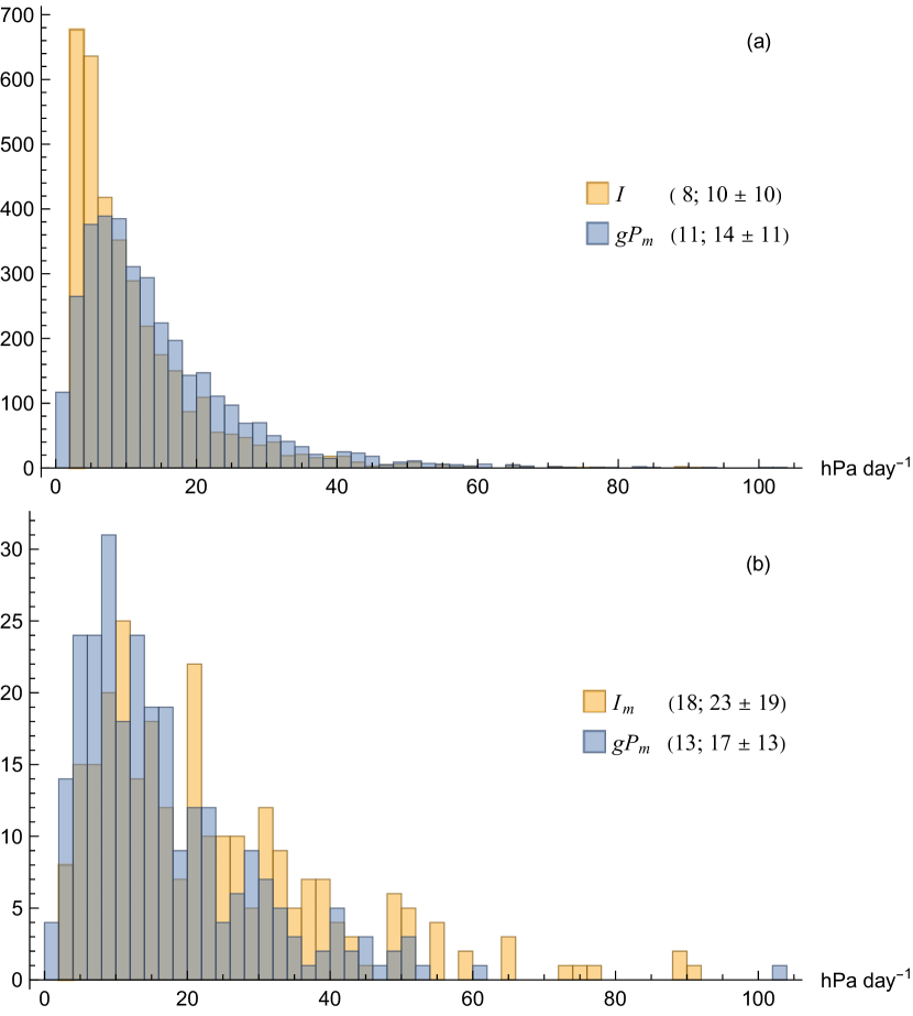
Figure 1: Frequency distribution of intensification rates $I$ (yellow) and concurrent maximum precipitation $gP_{m}$ (blue) in North Atlantic cyclones in $1998$–$2015$. Figures in brackets are (median; mean $\pm$ standard deviation) (hPa day^-1). (a) All $3492$ records for intensifying storms ($I>0$); (b) Lifetime maximum intensification rates $I_{m}$ and concurrent maximum precipitation $gP_{m}$ for $266$ individual storms. Two extreme values $I=I_{m}=166$ hPa day^-1 and $I=128$ hPa day^-1 recorded for hurricane Wilma $2005$ are not shown but included in the statistics.

For numerical modeling we used CM1 release 20.3 (Bryan and Fritsch, 2002). We used the default configuration for the axisymmetric runs (provided in the “hurricane_axisymmetric” directory of the model configuration) with the following minimal modifications. We used $\rm ptype=6$ for the “simple Rotunno-Emanuel (1987) water-only scheme” (Rotunno and Emanuel, 1987). We set terminal velocity $V_{t}=0$ for reversible (REV) and $V_{t}=-10$ for pseudoadiabatic (PSE) runs. In the CM1 model, negative $V_{t}$ with $\rm ptype=6$ correspond to the pseudoadiabatic regime when the condensate is immediately removed from the atmosphere.

Additionally, we used a model run termed NOEV, where condensate did not fall out and the evaporation of cloud water in the atmosphere was switched off by changing the line “IF(q3d(i,j,k,nqc).gt.1.0e-12 .or. q3d(i,j,k,nqv).gt.qvs)THEN” to “IF(q3d(i,j,k,nqv).gt.qvs)THEN” in the $\rm satadj$ subroutine.

As the initial temperature and moisture profiles, for REV and NOEV we used the reversible profile, and for PSE we used the control profile from Wang and Lin (2020, their Fig. 1) that both correspond to a surface air temperature $T_{a}=296.15$ K. Sea surface temperature was set to $T_{s}=306.15$ K and $T_{s}=301.15$ K for REV and NOEV and for PSE, respectively, such that the difference $\Delta T_{s}\equiv T_{s}-T_{a}$ was $10$ K for REV and NOEV and $5$ K for PSE.

We analyze the results of simulations for $400$ hours, which exceeds the lifetime of more than $95\%$ of real tropical cyclones (Lee et al., 2016, their Supplementary Fig. 2). All information necessary to replicate our simulations, as well as the $P(r)$ distributions for individual storm records, can be found at https://doi.org/10.5281/zenodo.10577109.

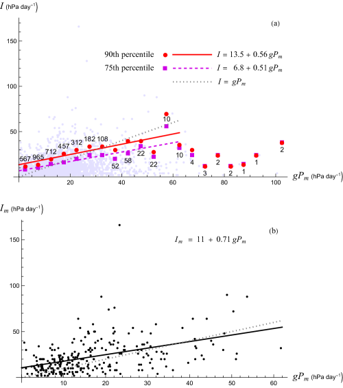
Figure 2: Dependence between intensification rates and maximum precipitation. (a) Linear regressions on $gP_{m}$ of the $90$th and $75$th percentiles of $I$ in $5$ hPa day^-1 bins of $gP_{m}$ with $n\geq 10$. Numbers $n$ of $I$ values in each bin are shown. Small dots are all $I$ values. (b) Linear regression of lifetime maximum intensification $I_{m}$ on $gP_{m}$. Dotted lines $I=gP_{m}$ (a) and $I_{m}=gP_{m}$ in (b) are shown for reference. In (b), one outlier (Hurricane Omar 2008 with $gP_{m}=102$ hPa day^-1 and $I_{m}=38$ hPa day^-1) is neither shown nor taken into account in the regression of $I_{m}$ on $gP_{m}$.

3 Intensification and precipitation in North Atlantic tropical cyclones

Intensification rates $I$ and maximum local precipitation $gP_{m}$ are on average close in magnitude being both of the order of $10$ hPa day^-1 (Fig. 1). Their frequency distributions differ in that $I$ has a higher peak at lower values (Fig. 1a): there are more cases of slowly intensifying storms than of intensifying storms with low precipitation. For lifetime maximum intensification rates $I_{m}$ this feature is not present, the means of $I_{m}$ and $gP_{m}$ are both close to $20$ hPa day^-1 (Fig. 1b). The median $I_{m}=18$ hPa day^-1 for $266$ intensifying North Atlantic storms that happened in $1998$–$2015$ is comparable to the median $I_{m}=24$ hPa day^-1 for $305$ North Pacific storms that happened in $1956$–$1976$ (Holliday and Thompson, 1979). Note, however, that our $I$ and $I_{m}$ were defined using a period of twelve hours rather than twenty four as in (Holliday and Thompson, 1979).

The quantitative similarity between $I$ and $gP_{m}$ is not limited to their means. In $5$ hPa day^-1 bins of $gP_{m}$, the $90$th and $75$th percentiles of $I$ grow with $gP_{m}$ (Fig. 2a). Lifetime maximum intensification rates $I_{m}$ also increase with $gP_{m}$ (Fig. 2b). The intercepts at zero precipitation are around $10$ hPa day^-1.

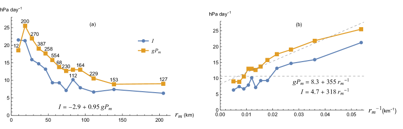
Figure 3: Dependence of intensification rate $I$ and maximum concurrent precipitation $gP_{m}$ on the radius of maximum wind (a) and inverse radius of maximum wind (b). Mean values of $I$ and $gP_{m}$ in each bin of $r_{m}$ are shown versus mean values of $r_{m}$ (a) and $r_{m}^{-1}$ (b) in each bin. Numbers $n$ of $I$ and $gP_{m}$ pairs of values in each bin are shown. Linear regression of the mean values of $I$ and $gP_{m}$ is shown in (a). In (b), the bin with the smallest $r_{m}$ and the smallest $n=12$ is neither shown nor taken into account in the regressions of $I$ and $gP_{m}$ on $r_{m}^{-1}$.

Figure 3 shows that both intensification rate and maximum concurrent precipitation depend similarly on the radius of maximum wind, with $gP_{m}$ being at all but the smallest $r_{m}$ larger than $I$ by approximately $4$ hPa day^-1.

We emphasize that we are not just dealing with a positive correlation between $I$ and $gP$, but with their numerical equivalence. Central pressure is diminishing approximately as it would if the inflow and outflow at the radius of maximum precipitation were exactly compensated, $F_{\rm in}=F_{\rm out}$, and surface pressure within this radius declined at a rate dictated by precipitation alone. This simplified picture certainly has its limitations, as surface pressure does not decline uniformly everywhere within the radius of maximum precipitation.

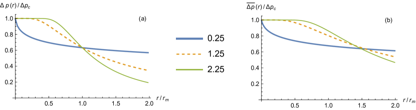
Figure 4: Dimensionless Holland’s pressure profile $\Delta p(r)$, Eq. (3), and the mean pressure drop $\overline{\Delta p}(r)=2r^{-2}\int^{r}_{0}\Delta p(r^{\prime})r^{\prime}dr^{\prime}$ within a circle of a given radius for three values of $b=0.25$, $1.25$, and $2.25$.

Using Holland’s pressure profile

$$\Delta p(r)\equiv p(\infty)-p(r)=\Delta p_{c}\left[1-\exp\left\{-\left(\frac{r_{m}}{r}\right)^{b}\right\}\right],$$ (3)

where $\Delta p(r)>0$ and $\Delta p_{c}>0$ are the surface pressure drop at radius $r$ and the storm center $r=0$, respectively, $b\sim 1$ is a scaling parameter (Holland, 1980; Vickery and Wadhera, 2008; Holland et al., 2010, their Eq. (2)). At the radius of maximum wind $r=r_{m}$, the pressure drop does not depend on $b$: $\Delta p_{m}\equiv\Delta p(r_{m})=(1-e^{-1})\Delta p_{c}\simeq 0.6\Delta p_{c}$ (Fig. 4a). Likewise, the mean pressure drop $\overline{\Delta p}$ does not depend on $b$ at $r\simeq 1.5r_{m}$ where it also constitutes about $0.6\Delta p_{c}$ (Fig. 4b).

If this relationship holds during intensification, one can expect that within the circle $r\leq 1.5r_{m}$ the mean pressure tendency $I(1.5r_{m})\equiv\partial\overline{\Delta p}(1.5r_{m})/\partial t$ will be by a factor of about $0.6$ smaller than $I\equiv\partial\Delta p_{c}/\partial t$, $I(1.5r_{m})\simeq 0.6I$.

The radius of maximum precipitation $r_{P}$ is close to $1.5r_{m}$ in tropical cyclones of category $1$-$3$ and about $r_{P}\simeq 1.2r_{m}$ in the more intense and in the less intense cyclones (Wang et al., 2024, their Fig. 2). If $I(1.5r_{m})$ is approximately determined by $g\overline{P}(r_{P})$, then we can expect $g\overline{P}(r_{P})\simeq 0.6I_{m}$. Figure 5 shows that the medians and means of $0.6I_{m}$ and $g\overline{P}(r_{P})$ are very close. These spatial patterns require further study.

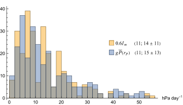
Figure 5: Frequency distribution of lifetime maximum intensification rates $I_{m}$ multiplied by a factor $0.6$ (yellow) and mean precipitation $g\overline{P}(r_{P})$ within the radius $r_{P}$ of maximum precipitation (blue) in $266$ North Atlantic cyclones in $1998$–$2015$. Figures in brackets are (median; mean $\pm$ standard deviation) (hPa day^-1). Two extreme values, $I_{m}=166$ hPa day^-1 for hurricane Wilma $2005$ and $g\overline{P}(r_{P})=102$ hPa day^-1 for Hurricane Omar $2008$, are not shown but taken into account in the statistics.

4 Intensification of model storms without a mass sink

While in real life latent heat release is not separable from the condensation mass sink, numerical models represent a convenient tool to study the two effects separately. Our approach was not to do any tampering with the model parameters, but to use the default values of the CM1 model that, under realistic atmospheric conditions, would produce a realistic axisymmetric storm. Figure 6 shows that when the mass sink is switched off and the condensate does not fall out, the resulting reversible storm develops significantly more slowly than the storm with a condensation mass sink despite the greater temperature difference with the ocean in the former. In $400$ hours, the reversible storm develops a central pressure drop of $\Delta p_{c}=10$ hPa and maximum velocity $\upsilon_{m}=36$ m s^-1 (and continues to intensify). The pseudoadiabatic storm develops $\Delta p_{c}=128$ hPa and maximum velocity $\upsilon_{m}=107$ m s^-1 in $54$ hours and begins to deintensify slowly after $t=100$ h (a possible cause for this deintensification is the depletion of atmospheric moisture in the subsidence region, see Rousseau-Rizzi et al., 2021). By varying model setups, it is possible to make reversible storms develop more rigorously than the one shown in Fig. 6, but a drastic difference in the intensification rates persists (cf. Fig. 2 of Wang and Lin, 2020). Moreover, storms without condensation mass sink increase their radius of maximum wind as they intensify (Fig. 6c).

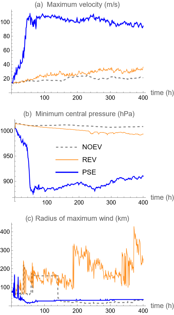
Figure 6: Intensification of a pseudoadabatic storm (PSE), reversible storm (REV) and a storm with evaporation in the air switched off (NOEV). The initial temperature difference with the ocean is $10$ K in REV and NOEV and $5$ K in PSE.

Let us consider a simplified qualitative picture of this intensification (Fig. 7a). The surface fluxes of water vapor and heat are parameterized as proportional to the absolute wind speed following Eqs. (34) and (35) of Rotunno and Emanuel (1987). Therefore, at the initial moment of time at the radius of maximum wind $r_{m}=80$ km of the initial tangential wind profile, the air is warming more intensely compared to the air at other radii. As this warmer air begins to rise, there forms an outflow governed by the pressure surplus caused by the higher temperature in the upper troposphere.

As the upper air flows away, surface pressure in the warmer region declines. This pressure drop causes an inflow in the lower atmosphere, which grows rapidly to match the outflow. The inflow is “slaved” to the outflow as it is a function of the pressure drop created by the outflow. Accordingly, intensification continues as long as the outflow and the surface pressure drop it creates increase. Intensification is related to increasing temperature (Schubert and Hack, 1982; Emanuel et al., 1994): the outflow grows as long as the ascending air warms ($\partial T/\partial t>0$). As soon as thermal equilibrium is reached and $\partial T/\partial t=0$, the intensification stops. Apparently, in the heat-driven storm shown in Fig. 6, the hypothetical feedback between a decrease in the radius of maximum wind and an increase of latent heat release to cause $\partial T/\partial t>0$ and drive further intensification (the so-called increased latent heat efficiency), is not realized (Schubert and Hack, 1982; Smith and Montgomery, 2016b).

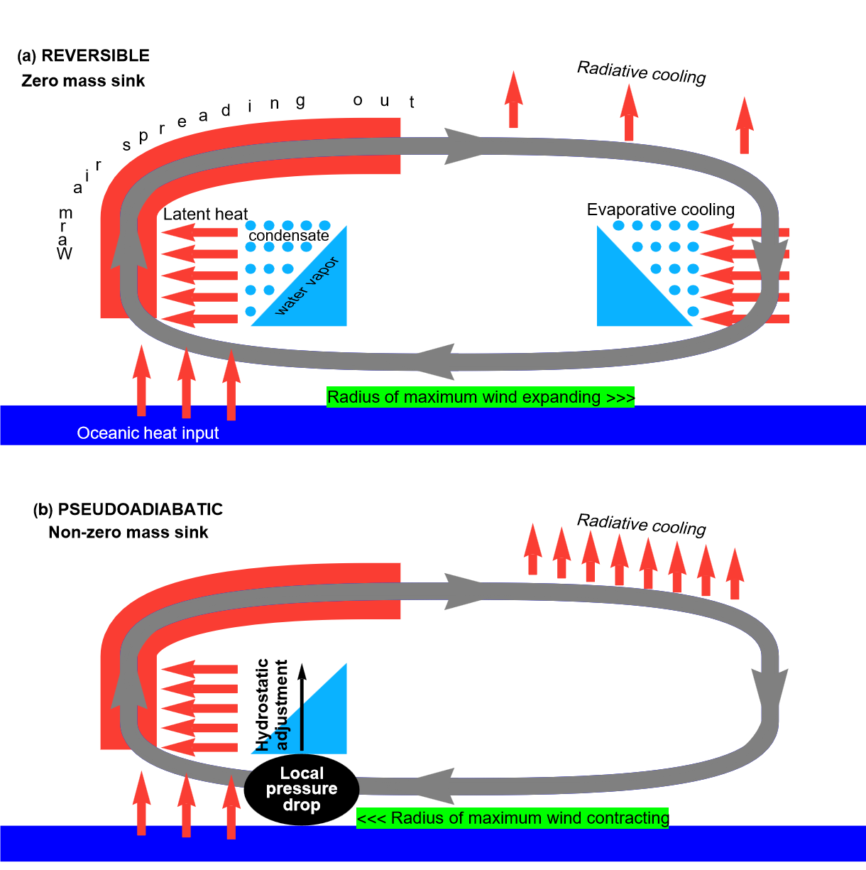
Figure 7: Key mechanisms at play during intensification of storms without (a) and with (b) condensation mass sink. In (b), since there is no condensate to evaporate, all latent heat released in the ascent region must be radiated to space in order for the air to descend.

What determines how slowly the storm intensifies? In this model setup, the atmosphere receives energy (in the form of latent and sensible heat) from the warmer ocean of constant temperature and loses energy via radiative cooling parameterized following Eq. (30) of Rotunno and Emanuel (1987):

$$Q_{r}=\frac{\theta-\overline{\theta}}{\tau_{r}}.$$ (4)

This relaxes the potential temperature profile $\theta(z,r)$ to the initial state $\overline{\theta}$. The time scale $\tau_{r}$ is chosen from the condition that the resulting cooling should approximately balance the subsidence region in realistic cyclones (such that $Q_{r}\simeq 2$ K day^-1).

Importantly, the descending air must lose all heat it has gained in the region of ascent. Otherwise it would end warmer at the surface than it started the ascent. The thermodynamic cycle would be characterized by negative work, as the air in the boundary layer would have to cool while moving from the subsidence region towards the region of ascent. This argument was comprehensively presented by Goody (2003). Accordingly, the subsidence must occur slowly enough for the air to dispatch all gained heat. But Kieu and Zhang (2009) showed that the intensification of tropical cyclones depends on how rapidly the secondary circulation intensifies. Thus, because secondary circulation (vertical velocity in the subsidence region) is limited by radiative cooling, the storm cannot develop faster than allowed by the cooling parameterization.

This limitation could be overcome, and the secondary circulation proceed more rapidly, if the storm core became more compact (the air can in principle ascend with an infinite velocity over an infinitely small area). But instead we can see that the radius of maximum wind grows (Fig. 6c). It grows because the horizontal profile of the pressure drop at the surface is determined by the warm outflow which naturally tends to expand rather than contract . As a result, in sharp contrast with real cyclones that generally reduce their $r_{m}$ during intensification (Willoughby, 1990; Li et al., 2021; Wu and Ruan, 2021), modeled cyclones without a mass sink increase their radius of maximum wind from the initial vortex with $r_{m}=80$ km to $r_{m}\gtrsim 200$ km (see Fig. 6c and Wang and Lin, 2020, their Fig. 2c).

5 Intensification of cyclones with a mass sink

5.a Latent heat handicap

Let us now consider how condensation mass sink modifies the intensification process (Fig. 7b). First, we note that in the subsidence region there is no condensate to evaporate. In the reversible storm, evaporative cooling in the descending air serves as a sink for the most part of the latent heat released in the region of ascent (Fig. 7a). In the absence of this heat sink, all this latent heat must now be radiated to space for the air to descend. This poses an even stricter limitation on the vertical velocity of subsiding air, which, for the same upward mass flow, should be several times less than in the reversible storm.

As we have already noted, the only way a storm can rapidly intensify under the strict limitation imposed by the need to get rid of the latent heat in the slowly descending air is by becoming more compact in the region of ascent. Wang and Lin (2021) expressed this idea by relating storm compactness to irreversibility (associated with the lack of evaporative cooling in the descending air). However, irreversibility by itself cannot make the storm more compact. An irreversible storm must be more compact if it is to develop. But it may not develop at all if there is no dynamic process that ensures its compaction.

To illustrate this simple idea, we introduced irreversibility by switching off the evaporation of condensate while keeping all condensate in the air (model run NOEV in Fig. 6). In this case there is no storm development. The circulation is unable to dispose of a huge amount of latent heat which therefore serves as a break on its intensification. Condensation mass sink absent, the storm cannot get more compact whether it is irreversible or not.

5.b Outflow by centrifugal force

Condensation mass sink apparently provides for the needed compaction. As the warmer air begins to rise and flow away from the cylinder of radius $r=r_{m}$, there is now a distinct additional process to remove mass from the column and lower surface pressure: precipitation. In contrast to the temperature-driven outflow that tends to equalize the temperature difference across the domain which results in storm expansion, the mass sink reduces surface pressure locally – where precipitation actually occurs.

As in all storms, the inflow is driven by the surface pressure drop. But the surface pressure drop is now driven not only by an increase in the outflow due to rising temperature, but also by the mass sink. For inflow and outflow to remain closely coupled, there must be an outflow process that correlates with the inflow driven by the mass sink. This outflow is caused by the centrifugal force, which ventilates away all the air that rises high enough. Indeed, in both models (Kurihara, 1975; Smith et al., 2018; Makarieva et al., 2023) and observations (He et al., 2018, 2019, their Fig. 7), the radial pressure gradient is positive in the upper outflow region (around $12$ km) and serves as a sink of kinetic energy generated in the boundary layer.

Whether the centrifugal force is able to ventilate the upper air can be assessed as follows. Kinetic energy per unit mass of air is $\upsilon_{m}^{2}/2$, where $\upsilon_{m}$ is the maximum tangential velocity. It is observed in the narrow inflow layer near the surface. Applying Bernoulli’s equation (e.g., Emanuel, 1991, his Eq. (1)) to the horizontal streamline, we can write

$$\frac{\upsilon_{m}^{2}}{2}=k\frac{\Delta p_{m}}{\rho_{s}},$$ (5)

where $\rho_{s}=1$ kg m^-3 is surface air density, $\Delta p_{m}>0$ is the surface pressure drop at the point of maximum wind and factor $k\lesssim 1$ reflects the kinetic energy loss due to friction. Taking into account that at the radius of maximum wind the surface air is in (approximate) gradient-wind balance:

$$\frac{\partial p}{\partial r}\Big{|}_{r=r_{m}}=\rho\frac{\upsilon_{m}^{2}}{r_{m}},$$ (6)

using Holland’s pressure profile, Eq. (3), and solving Eqs. (5) and (6) for $r=r_{m}$ and $k=k(b)$, we obtain (cf. Vickery and Wadhera, 2008, their Eq. (4)):

$$k=\frac{b}{2(e-1)}.$$ (7)

For the range of $0.25\leq b\leq 2.25$ as per Holland’s (1980) Fig. 2 we obtain $0.07\leq k\leq 0.65$. With a mean $b\simeq 1.25$ (Vickery and Wadhera, 2008), we have $k\simeq 0.4$. This means that more than one third of the potential energy of the pressure drop along the streamline from the storms outskirts to the radius of maximum wind is converted to kinetic energy. It is a big proportion. For Hadley cells, for example, with a typical pressure difference $\Delta p=10$ hPa and maximum velocity $\upsilon=7$ m s^-1, we would have $k\sim 0.02$.

The value $|\Delta p(z)|/\rho(z)$, where $\rho(z)$ is local air density and $\Delta p(z)\equiv p(\infty,z)-p(r,z)$ is the pressure difference between the unperturbed external environment and the local point, is equal to the minimum kinetic energy required to move air against this pressure difference from the eyewall to the external environment. If this energy is less than $\upsilon_{m}^{2}/2$, the outflow of air by the centrifugal force is energetically permitted. Maximum possible outflow $U(z)\rho(z)$ is obtained from the condition that all kinetic energy is spent on the radial motion with velocity $U(z)$:

$$U(z)=\sqrt{2k\frac{\Delta p_{m}}{\rho_{s}}-2\frac{\Delta p(z)}{\rho(z)}}.$$ (8)

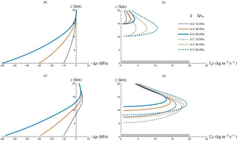
Figure 8: Vertical pressure differences $\Delta p(z)\equiv p_{0}(z)-p(z)$ (a,c) and the corresponding profiles $U(z)\rho(z)$ (b,d) calculated from Eq. (8), where $p(z)$ is the vertical pressure of moist saturated air columns with a pseudoadiabatic lapse rate, surface air temperature $T_{s}=298$ K and a surface pressure deficit of $\Delta p_{m}=10$, $30$ and $60$ hPa compared to the reference surface pressure $p_{0}(0)=10^{3}$ hPa. In (a), the reference pressure profile is a moist saturated air column with a pseudoadiabatic lapse rate and $T_{s}=298$ K; in (b) it is an air column with $T_{s}=300$ K and relative humidity $80\%$ at the surface; with dry adiabatic lapse rate up to the dew point at $z=474$ m and a moist pseudoadiabatic profile above.

Figure 8a,b describes a case when both the eyewall and the external environment have a moist pseudoadiabatic vertical temperature profile with the same surface temperature $T_{s}=298$ K, but the eyewall has a surface pressure deficit of $\Delta p_{m}=10$, $30$ or $60$ hPa compared to the external environment. In this case, the air pressure in the eyewall is lower than in the external environment at all heights below approximately $20$ km (Fig. 8a). The gray bar in Fig. 8b,d illustrates a typical magnitude of the low-level inflow $u_{\rm in}\rho_{s}h_{\rm in}$: height of the inflow layer $h_{\rm in}=1$ km, horizontal velocity $u_{\rm in}=20$ m s^-1, and air density $\rho_{s}=1$ kg m^-3.

For an equal outflow to be energetically permitted, the area to the left of the $U(z)\rho(z)$ curves in Fig. 8b,d should be equal to or greater than that of the gray bar. Figure 8a,b indicates that at the highest $k=0.7$ the centrifugal force is able to ensure an adequate outflow between $10$ and $15$ km. This is where the outflow predominantly occurs in both real and modeled cyclones (Miller, 1958; Frank, 1977; Smith et al., 2018). For a given $k$, this energetically permitted outflow increases with increasing pressure deficit at the surface $\Delta p_{m}$. At lower $k=0.3$ (less kinetic energy available for a given $\Delta p_{m}$) the air has to rise five kilometers higher and still there does not seem to be enough kinetic energy for it to be ventilated by the centrifugal force alone.

Figure 8c,d shows a case where the eyewall has a small pressure surplus aloft not exceeding $2$ hPa between $10$ and $20$ km similar to the height-resolving pressure profiles for tropical cyclones established by He et al. (2019, their Fig. 7). The external environment is represented by an atmospheric column with $T_{s}=300$ K (i.e., it is by $2$ K warmer at the surface than the eyewall) but is unsaturated at the surface at $80\%$ relative humidity. Even as the eyewall is colder at the surface (which may reflect the adiabatic expansion of inflowing air), its greater moisture content allows for a higher temperature aloft that is responsible for the pressure surplus shown in Fig. 8c. Accordingly, the energetically permitted outflow increases, cf. Fig. 8b,d. Now even at a lower $k=0.3$ the air can be ventilated if it rises to about $10$ km. Note that in this case for a given $k$ the higher the surface pressure deficit, the higher the air must rise to be ventilated. For example, with $k=0.7$ and $\Delta p_{m}=10$ hPa, the air can be ventilated from above $5$ km, while with $\Delta p_{m}=60$ hPa it must rise to above $8$ km. Figure 9 shows that during the storm development the pressure surplus aloft can be present at early stages but disappear later as the storm deepens.

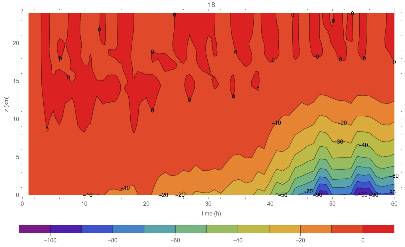
Figure 9: Time evolution of the difference $\Delta p(z)$ (hPa) between the vertical pressure profile at the radius of maximum wind and the outermost model radius in the PSE run during the first sixty hours of development. Note a small pressure surplus ($\lesssim 1$ hPa) in the upper troposphere at early stages of development and its disappearance later.

5.c Condensation, pressure adjustment and storm (de)-intensification

Figure 8 suggests that if the air rises sufficiently high, there is no problem for it to be ventilated from the eyewall under realistic atmospheric conditions. However, if the ascending motion is compromised, so will be the outflow. From this position – whatever rises flows away, and whatever does not rise does not flow away – we can conceptualize the role of pressure adjustment that occurs during condensation in generating negative and positive pressure tendencies (Fig. 10).

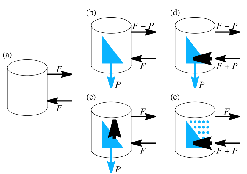
Figure 10: The role of pressure adjustment accompanying condensation in generating pressure tendencies. The triangle symbolizes the non-equilibrium vertical distribution of the partial pressure of water vapor that results from condensation; $P$ is precipitation, $F$ is the absolute steady-state magnitude of the inflow (the lower thin horizontal arrow) from the eyewall (cylinder) and outflow $F_{\rm out}$ (the upper thin horizontal arrow) that are assumed to be balanced in the absence of the condensation (a). Thick black arrows indicate the vertical (hydrostatic) pressure adjustment in (c) and the horizontal pressure adjustment in (d) and (e). The pressure tendency $(1/g)\partial p/\partial t=F_{\rm in}-F_{\rm out}-P$ is equal to zero in (a) and (b), to $-P$ in (c) and to $+P$ in (d) and (e), see text for details.

We consider condensation mass sink as a perturbation to the steady-state heat-driven circulation where the inflow and outflow are exactly balanced, $F_{\rm in}=F_{\rm out}=F$ and $\partial p/\partial t=0$ (Fig. 10a). A salient feature of the condensation mass sink is the formation of a strongly non-equilibrium vertical gradient of the partial pressure of water vapor. In a hypothetical case of no pressure adjustment to accompany condensation, this non-equilibrium would reduce the outflow by the magnitude of precipitating moisture, $F_{\rm out}=F-P$. Instead of rising to be ventilated, water vapor would be exiting the column by condensation and precipitation. As a result, the pressure tendency equal to $(1/g)\partial p/\partial t=F_{\rm in}-F_{\rm out}-P=0$ would remain zero (Fig. 10b).

Hydrostatic adjustment redistributes the air upwards such that the void caused by condensation is occupied by the air from below. If the hydrostatic adjustment pushes the air sufficiently high up (this vertical scale is governed by the mean precipitation height $H_{P}$, Makarieva et al., 2013a), then the outflow can regain its steady-state unperturbed value $F_{\rm out}=F$. Instead of rising to be ventilated, water vapor condenses and precipitates, but its place is occupied by the dry air pushed up by the hydrostatic adjustment. In this case, the pressure tendency is negative, $(1/g)\partial p/\partial t=F_{\rm in}-F_{\rm out}-P=-P$ (Fig. 10c). The storm intensifies.

But it is also possible, especially if the eyewall is narrow and/or the mean precipitation height is low, that the predominant direction of the pressure adjustment will be in the horizontal plane (Fig. 10d). This will increase the inflow $F_{\rm in}$ to $F+P$ (the absolute magnitude of radial velocity will grow by the so-called barycentric velocity, see discussion by Makarieva et al., 2013b) and can cause a positive pressure tendency of the same magnitude, $(1/g)\partial p/\partial t=F_{\rm in}-F_{\rm out}-P=+P$ (Fig. 10d). Horizontal adjustment can be compared to the “back pressure” as formulated by Lindzen and Nigam (1987) but probably on a shorter timescale. When the condensate does not fall out, the horizontal pressure adjustment is possible, while the vertical adjustment is not (Fig. 10e). This illustrates why it is difficult for the reversible storm to intensify.

This ability of water vapor condensation to generate both positive and negative pressure tendencies of (at maximum) the same absolute magnitude determined by precipitation, depending on the geometry of the pressure adjustment, is quite remarkable. It can provide a clue to the very peculiar pattern of intensification and de-intensification rates in real storms having approximately the same mean magnitudes (Fig. 11). They also depend similarly on the radius of maximum wind (Sparks and Toumi, 2022b) and by inference on precipitation (cf. Fig. 3).

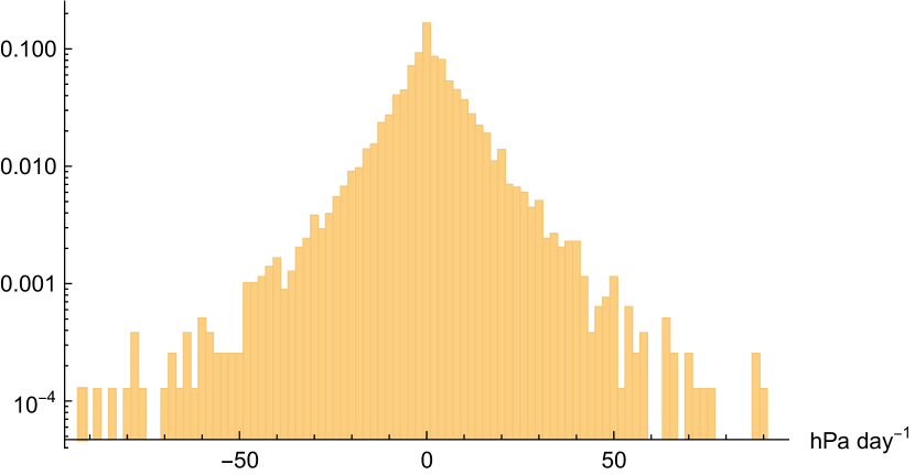
Figure 11: Frequency distribution of all $7848$ values of intensification rates including both intensifying (positive values) and de-intensifying (negative values) storms, mean value is $\overline{I}=0.7\pm 13$ hPa day^-1. Six outliers with $-112$ hPa day^-1 $\leq I\leq-96$ hPa day^-1 and two outliers with $I=166$ hPa day^-1 and $I=128$ hPa day^-1 are not shown.

This is peculiar, because model storms do not de-intensify at the same rate they intensify but tend to reach a steady state (e.g., see discussion by Rousseau-Rizzi et al., 2021). This agrees with the idea that such a state is a stable attractor (Kieu, 2015). Indeed, if intensification of tropical storms is governed by self-induced dynamics characterized by its own timescale that is comparable to the storm’s lifetime (e.g., as shown in Fig. 2 of Schubert and Hack, 1982), why would their de-intensification occur at a similar rate? The concept presented in Fig. 10 allows one to hypothesize that the intensification and de-intensification of the storm can be, in the zeroth approximation, viewed as a pulsation where the vertical pressure adjustment dominates during intensification and the horizontal adjustment during de-intensification. This said, we acknowledge the complexity of these matters and previous discussions (e.g., Kowch and Emanuel, 2015; Lee et al., 2016; Sparks and Toumi, 2022b) and emphasize the need for further studies.

How could the switch between the two regimes occur? The mean condensation height for complete condensation in the tropical atmosphere is about $6$ km (Makarieva et al., 2013a). As Figure 8d shows, with increasing surface pressure deficit in the eyewall $\Delta p_{m}$, height of the lower boundary of the outflow layer increases. As the storm deepens, when the lower boundary of the outflow significantly exceeds the condensation height, we can hypothesize that hydrostatic adjustment will be unable to push the air high enough to keep the outflow unperturbed. Thus as the cyclone intensifies, on the one hand, the radius of maximum wind $r_{m}$ decreases and precipitation increases, and this enhances intensification. On the other hand, as the surface pressure deficit in the eyewall becomes too high, the difference between precipitation height $H_{P}$ and the lower boundary of the outflow layer increases, and the intensification can stop. This may explain the fact that high-intensity cyclones like hurricanes of 3-5 category undergo rapid intensification several times less often than the less intense storms (Wang et al., 2024).

When the horizontal adjustment becomes dominant over the hydrostatic adjustment is a difficult theoretical question (Chagnon and Bannon, 2005; Spengler et al., 2011). However, it is clear that the horizontal scale of the maximum precipitation area should play a role. As the storm becomes more compact and the eyewall width becomes less than $H_{P}$, horizontal adjustment should come into play and de-intensification commence. This can determine the minimal eyewall radius (of a few kilometers) that the most intense storms can attain.

On the other hand, the more complete condensation, the higher the mean precipitaiton height (Makarieva et al., 2013a, their Fig. 1). This may explain why high convective bursts are known to be associated with rapid intensification (e.g., Chen and Zhang, 2013). If $H_{P}$ grows abruptly and becomes higher than the lower boundary of the outflow layer, this can initiate rapid intensification. The subtle interplay between $H_{P}$, $\Delta p_{m}$, $r_{m}$ and $r_{P}$ that can cause the switch between intensification and de-intensification makes prediction of rapid intensification a challenging matter (cf. "the subtle vertical structure issues" sensu Masunaga and Mapes, 2020, p. 1182).

6 Discussion and conclusions

We have shown that the lifetime maximum intensification rates in North Atlantic tropical cyclones approximately coincide with local maximum precipitation and that turning off precipitation in the CM1 model greatly reduces the intensification rates. If one is not ready to immediately accept a major role for the condensation mass sink in storm dynamics, one faces the challenge of providing alternative explanations. For example, if tropical cyclones intensify by WISHE (wind-induced surface heat exchange) or by vortical hot towers (Montgomery et al., 2009), what clues do the respective concepts provide to anticipate that reversible cyclones (i.e., those with maximum thermodynamic efficiency) will not develop at all when the temperature difference between the ocean and the air is less than $5$ K (Wang and Lin, 2020), and when they will slowly develop, they will expand rather than contract? Understanding why storms do not intensify can be inseparable from understanding why they do.

The correspondence between intensification rate and precipitation is not the first indication of condensation mass sink possibly playing a major role in tropical storm dynamics. Makarieva and Gorshkov (2007) proposed that the non-equilibrium vertical distribution of water vapor partial pressure, which is compressed sixfold as compared to the hydrostatic distribution, represents a source of potential energy to drive winds. This proposition (termed condensation-induced atmospheric dynamics) was later elaborated and found to be relevant in the context of hurricanes and tornadoes (Makarieva and Gorshkov, 2009, 2011; Makarieva et al., 2011; Gorshkov et al., 2012; Makarieva et al., 2015). In particular, the scale for the maximum velocity $\upsilon_{m}$ is given by $\rho\upsilon_{m}^{2}/2=p_{\upsilon}$, where $\rho$ is air density and $p_{\upsilon}$ is partial pressure of water vapor that is interpreted as the maximum available potential energy. For typical temperatures $T=300$ K and relative humidity $80\%$ we have $p_{\upsilon}\simeq 35$ hPa which, with $\rho=1$ kg m^-3, gives $\upsilon_{m}\simeq 80$ m s^-1 corresponding to a category 5 hurricane.

Furthermore, if condensation of water vapor releases $p_{\upsilon}/N_{\upsilon}=RT$ (J mol^-1) of potential energy ($R=8.3$ J mol^-1 K^-1 is the universal gas constant, $N_{\upsilon}=\rho_{\upsilon}/M_{\upsilon}$ is the molar density of water vapor), which is converted to kinetic energy and locally dissipates, then the local dissipation rate should be given by $PRT/M_{\upsilon}$ (Makarieva and Gorshkov, 2011; Makarieva et al., 2015). For $P=200$ kg m^-2 day^-1 this gives $320$ W m^-2. This coincides with the independently estimated dissipation rate $\rho C_{D}\upsilon_{m}^{3}\simeq 300$ W m^-2 of an average Atlantic hurricane with $\upsilon_{m}=50$ m s^-1, where $C_{D}=2\times 10^{-3}$ is a characteristic surface drag coefficient (Emanuel, 1999). Notably, for global precipitation $P=1$ m year^-1, the same expression $PRT/M_{\upsilon}=4$ W m^-2 yields a magnitude that is within $30\%$ of the global wind power, $3$ W m^-2, independently estimated from observed wind speeds and pressure gradients (Makarieva et al., 2013a, 2017b).

We believe that the new evidence in favor of a major role of the condensation mass sink in storm dynamics that we have presented justifies more attention to those arguments. We will conclude our discussion by placing the condensation mass sink into a broader atmospheric context.

Kieu (2004, 2006) showed that a realistic analytical solution for hurricane intensification could be obtained by postulating a positive feedback between the rate of latent heat release and vertical velocity. This is equivalent to assuming that the faster latent heat is released in the rising air, the warmer the atmospheric column, the greater the buoyancy, and as a result the air rises even faster (see Kieu, 2004, his Eq. 1.5’). However, Emanuel et al. (1994), see also discussion by Stevens et al. (1997) and Emanuel et al. (1997), pointed out that just because moisture condenses faster, it does not follow that the air gets warmer. In a subsequent publication, Kieu and Zhang (2009) showed that an analytical solution for hurricane intensification could be obtained by postulating an exponential growth of the vertical velocity, but at this point they already did not emphasize that this assumption could actually reflect a (problematic) positive feedback between latent heat release and vertical velocity [cf. Eq. (1.7) of Kieu (2004) and Eq. (6) of Kieu and Zhang (2009)].

A certain lack of clarity on this point apparently persists in the literature. For example, Chen and Zhang (2013, p. 147) opined that “clearly, the more intense the warm core, the greater will be the hydrostatically induced surface pressure falls”, with the core intensity quantified as the updraft velocity. This is despite Emanuel et al. (1994, p. 1140) warned that “disturbance growth requires a positive correlation of heating and temperature, and perturbations of the latter are usually very small, so that knowledge of the heating may be of little conceptual or predictive value.”

Some clues are provided by the earlier discussions of circulations driven by external differential heating or by latent heat release (e.g., Lindzen and Nigam, 1987; Neelin, 1989; An, 2011). External differential heating leads to a local increase in atmospheric scale height and vertical motion. There is a positive relationship: the greater the external heating, the greater the vertical motion due to increased temperature. As for latent heating, the positive relationship is different: the greater the vertical motion, the greater the latent heat release. This relationship has a different physical cause: it exists because the temperature gradient in the troposphere is approximately vertical, so condensation occurs predominantly as the air rises and cools. In neither case there is a positive feedback. In the first case, greater vertical velocity does not increase external differential heating (i.e., rising air does not make the sun brighter). In the second case, faster release of latent heat does not increase vertical velocity. But if the difference between latent heating and external heating is overlooked, it might appear that a positive feedback does exist.

Levermann et al. (2009, 2016) assumed a positive feedback between latent heat release and air motion to explain the enigmatic abrupt changes in the monsoon circulations of the past climates, but Boos and Storelvmo (2016b), see also Boos and Storelvmo (2016a), clarified, with a reference to Emanuel et al. (1994), that this assumption was not plausible. More recently, see Vallis and Penn (2020, their Eq. (2)), Davison and Haynes (2022) and Vallis (2022), showed that the same positive feedback between latent heat release and atmospheric warming can generate atmospheric patterns resembling the Madden-Julian Oscillation, a phenomenon that, like the rapid intensification of tropical storms, still defies a theoretical explanation.

Overall, it appears that positive feedback between condensation and atmospheric motion could be useful in elucidating several important problems in atmospheric science (besides tropical storms, monsoons and the Madden-Julian Oscillation, see also Masunaga and Mapes, 2020). However, theoretical studies in this direction are currently precluded by the valid objection that latent heat does not provide such feedback (Emanuel et al., 1994; Boos and Storelvmo, 2016b). But the condensation mass sink does. With the pressure tendency proportional to precipitation, it should be possible to show that the derivations that previously assumed a positive feedback between latent heat release and vertical velocity will largely retain their form but acquire a different, and plausible, physical meaning. This is immediately clear in the case of the shallow-water equations like Eq. (2) of Vallis and Penn (2020) which, in the framework of condensation-induced atmospheric dynamics, would be equivalent to $(1/g)\partial p/\partial t=-P$ (radiative cooling increasing the pressure tendency can play the role of horizontal pressure adjustment, cf. Fig. 10d).

The difference in intensification rates and maximum intensities of storms with and without the condensation mass sink shown in Fig. 6 can depend on model settings and especially on turbulence parameterization. In the CM1 model, turbulence parameters are determined from the condition that the resulting storm should be realistic. In the simulations of Wang and Lin (2020), who used a 3D model and different turbulence parameters than the default axisymmetric setup used in our study, the dry and reversible storms developed more rigorously than the reversible storm shown in Fig. 6. Using an older CM1 version and $\Delta T_{s}=13$ K, Rousseau-Rizzi et al. (2021) could obtain a dry storm that developed at a comparable rate with the control with a mass sink. Another observation is that storm intensity increases with increasing spatial resolution, both in CM1 (Bryan and Rotunno, 2009) and in global climate models (Daloz et al., 2015). Vallis and Penn (2020) likewise noted that for the self-sustained circulation mode to be preserved at shorter time steps, the horizontal resolution had to be increased (the grid size reduced). Conversely, Lindzen and Nigam (1987) noted that moisture convergence that was too high at a higher resolution came closer to observations when the grid size was increased.

Since efforts to increase the spatial resolution of global climate models go hand in hand with re-formulation of turbulence, the question is whether the right dynamics is preserved by these procedures. Vallis (2022) pointed out that condensation is a rapid process occurring on a shorter time and a smaller spatial scale than resolved by any model. Given that the time and spatial scales at which relevant dynamics arise remain unknown, not every combination of model parameters will be able to capture it.

Conceivably, there can be model setups (unknown combinations of grid size, time steps, turbulence parameters) that, to a certain degree, suppress condensation-induced dynamics and enhance heat-driven dynamics, or vice versa. Such model setups will have different behaviors and generate different predictions for atmospheric phenomena involving condensation. For example, there are first indications that higher resolution models predict a smaller decline in the Amazon rainfall upon deforestation because of enhanced air convergence due to more sensible heat over deforested land (Yoon, 2023). This could be an example of an artificially enhanced heat-driven circulation as compared to the model with a lower resolution. Indeed, recent studies suggest that global climate models could be overestimating the (heat-driven) moisture transport to the drier regions on land (Simpson et al., 2023).

One way of assessing to what degree condensation-induced dynamics is taken into account in a given atmospheric context is by using the reversible setup (switching precipitation off by putting the condensate velocity equal to zero). No difference would indicate that condensation-induced dynamics is not captured in the model. Another way would be to use an artificial model where condensation is programmed as a temperature-dependent chemical reaction that does not change the amount of gas while releasing the same amount of heat, and compare the output of this artificial model with the output of more realistic models.

The bottomline is that finding the right combination of model parameters that would capture real atmospheric dynamics is not possible without recognizing that besides heat there is a distinct driver of atmospheric motions, the condensation mass sink. What determines the change between regimes when precipitation reduces or increases surface pressure (Fig. 10)? Is invigoration of convection by aerosols (Abbott and Cronin, 2021) an example of such a switch? We believe that focused theoretical and empirical studies of condensation-induced atmospheric dynamics are indispensable and urgent.

Datastatement

The raw data utilised in this study are available at Zenodo https://doi.org/10.5281/zenodo.10577109. These data were derived from the following resources available in the public domain: https://disc.gsfc.nasa.gov/datasets/TRMM_3B42_7/summary and https://rammb2.cira.colostate.edu/research/tropical-cyclones/tc_extended_best_track_dataset/.

Appendix A Mass balance in the atmospheric air column

We consider the storm as an axisymmetric vortex. The air mass $M$(kg m^-2) per unit surface area is given by the integral over the volume $V=HS$ of a cylinder with a height $H$ and a base of area $S$:

$$M\equiv\frac{1}{S}\int_{V}\rho dV,$$ (A1)

where $\rho=\rho_{d}+\rho_{\upsilon}$ is the moist air density (dry air and water vapor).

The convergence $C$ of air in the considered region is determined as follows:

$$C\equiv-\frac{1}{S}\int_{V}\mathrm{div}(\rho\mathbf{u})dV=-\frac{1}{S}\oint_{\sigma}\rho u_{n}d\sigma\equiv F_{\rm in}-F_{\rm out},$$ (A2)

where $\mathbf{u}$ is the vector of air velocity. Its component $u_{n}=(\mathbf{u}\cdot\mathbf{n})$ is directed along the outward unit normal $\mathbf{n}$ to the closed surface $\sigma$, which encloses the volume $V$. Flux $F_{\rm in}$ corresponds to the case when the air flows into the region ($u_{n}<0$). Flux $F_{\rm out}$ corresponds to the case when the air flows out of the region ($u_{n}>0$). Since $\rho\simeq 0$ at the height $z=H$ and $u_{n}=0$ at the Earth’s surface, atmospheric air convergence $C$ describes the net flux of air across the lateral surface of the cylinder.

The difference between evaporation $E$ and precipitation $P$ is

$$E-P\equiv\frac{1}{S}\int\limits_{V}\dot{\rho}_{\upsilon}dV\simeq-P,$$ (A3)

where $\dot{\rho}_{\upsilon}$ is the mass source/sink of water vapor. The contribution of evaporation ($\dot{\rho}_{\upsilon}>0$) is assumed to be negligibly small compared to that of condensation ($\dot{\rho}_{\upsilon}<0$), i.e., $E\ll P$.

The surface pressure tendency is determined by the rate of change of air mass (A1):

$$\frac{1}{g}\frac{\partial p}{\partial t}=\frac{\partial M}{\partial t}=C-P=F_{\rm in}-F_{\rm out}-P,$$ (A4)

where $g$ is the acceleration of gravity. In eq. (A4), the second equality takes into account the mass balance in the atmospheric column.

We assume that flux $F_{\rm in}$ flows into the volume through a surface $\sigma_{\rm in}$ of area $S_{\rm in}=2\pi rh_{\rm in}$, while flux $F_{\rm out}$ flows out of the volume through a surface $\sigma_{\rm out}$ of area $S_{\rm out}=2\pi rh_{\rm out}$. Here $h_{\rm in}$ and $h_{\rm out}$ denote the depth of the corresponding layers and $r$ is the radius of cylinder. Surfaces $\sigma_{\rm in}$ and $\sigma_{\rm out}$ can be spatially separated. The average values of the air fluxes can be written as follows

$$F_{\rm in}=\rho u_{\rm in}\frac{S_{\rm in}}{S}=2\rho u_{\rm in}\frac{h_{\rm in}}{r},\quad F_{\rm out}=\rho u_{\rm out}\frac{S_{\rm out}}{S}=2\rho u_{\rm out}\frac{h_{\rm out}}{r},$$ (A5)

where $S=\pi r^{2}$ and average velocities $u_{\rm in}=-u_{n}>0$ and $u_{\rm out}=u_{n}>0$.

References

- Abbott and Cronin (2021) Abbott, T. H. and Cronin, T. W.: Aerosol invigoration of atmospheric convection through increases in humidity, Science, 371, 83–85, 10.1126/science.abc5181, 2021.
- Aberson et al. (2006) Aberson, S. D., Montgomery, M. T., Bell, M., and Black, M.: Hurricane Isabel (2003): New insights into the physics of intense storms. Part II: Extreme localized wind, Bull. Amer. Meteor. Soc., 87, 1349–1354, 10.1175/BAMS-87-10-1349, 2006.
- An (2011) An, S.-I.: Atmospheric responses of Gill-type and Lindzen-Nigam models to global warming, J. Climate, 24, 6165–6173, 10.1175/2011JCLI3971.1, 2011.
- Boos and Storelvmo (2016a) Boos, W. R. and Storelvmo, T.: Near-linear response of mean monsoon strength to a broad range of radiative forcings, Proc. Natl. Acad. Sci. USA, 113, 1510–1515, 10.1073/pnas.1517143113, 2016a.
- Boos and Storelvmo (2016b) Boos, W. R. and Storelvmo, T.: Reply to Levermann et al.: Linear scaling for monsoons based on well-verified balance between adiabatic cooling and latent heat release, Proc. Natl. Acad. Sci. USA, 113, E2350–E2351, 10.1073/pnas.1603626113, 2016b.
- Bryan and Fritsch (2002) Bryan, G. H. and Fritsch, J. M.: A benchmark simulation for moist nonhydrostatic numerical models, Mon. Wea. Rev., 130, 2917–2928, 10.1175/1520-0493(2002)130<2917:ABSFMN>2.0.CO;2, 2002.
- Bryan and Rotunno (2009) Bryan, G. H. and Rotunno, R.: The maximum intensity of tropical cyclones in axisymmetric numerical model simulations, Mon. Wea. Rev., 137, 1770–1789, 10.1175/2008MWR2709.1, 2009.
- Chagnon and Bannon (2005) Chagnon, J. M. and Bannon, P. R.: Adjustment to injections of mass, momentum, and heat in a compressible atmosphere, J. Atmos. Sci., 62, 2749–2769, 10.1175/JAS3503.1, 2005.
- Chen and Zhang (2013) Chen, H. and Zhang, D.-L.: On the rapid intensification of Hurricane Wilma (2005). Part II: Convective bursts and the upper-level warm core, J. Atmos. Sci., 70, 146–162, 10.1175/JAS-D-12-062.1, 2013.
- Daloz et al. (2015) Daloz, A. S., Camargo, S. J., Kossin, J. P., Emanuel, K., Horn, M., Jonas, J. A., Kim, D., LaRow, T., Lim, Y.-K., Patricola, C. M., Roberts, M., Scoccimarro, E., Shaevitz, D., Vidale, P. L., Wang, H., Wehner, M., and Zhao, M.: Cluster analysis of downscaled and explicitly simulated North Atlantic tropical cyclone tracks, J. Climate, 28, 1333–1361, 10.1175/JCLI-D-13-00646.1, 2015.
- Davison and Haynes (2022) Davison, M. and Haynes, P.: Excitable Madden-Julian Oscillation like behaviour of a simple model of equatorial moist dynamics results from a time step that is too large, Quart. J. Roy. Meteor. Soc., 148, 770–777, 10.1002/qj.4229, 2022.
- Demuth et al. (2006) Demuth, J. L., DeMaria, M., and Knaff, J. A.: Improvement of advanced microwave sounding unit tropical cyclone intensity and size estimation algorithms, J. Appl. Meteor. Climatol., 45, 1573–1581, 10.1175/JAM2429.1, 2006.
- Emanuel (1988) Emanuel, K. A.: The maximum intensity of hurricanes, J. Atmos. Sci., 45, 1143–1155, 10.1175/1520-0469(1988)045<1143:TMIOH>2.0.CO;2, 1988.
- Emanuel (1991) Emanuel, K. A.: The theory of hurricanes, Annu. Rev. Fluid Mech., 23, 179–196, 10.1146/annurev.fl.23.010191.001143, 1991.
- Emanuel (1999) Emanuel, K. A.: The power of a hurricane: An example of reckless driving on the information superhighway, Weather, 54, 107–108, 10.1002/j.1477-8696.1999.tb06435.x, 1999.
- Emanuel et al. (1994) Emanuel, K. A., Neelin, J. D., and Bretherton, C. S.: On large-scale circulations in convecting atmospheres, Quart. J. Roy. Meteor. Soc., 120, 1111–1143, 10.1002/qj.49712051902, 1994.
- Emanuel et al. (1997) Emanuel, K. A., Neelin, J. D., and Bretherton, C. S.: Reply to comments by Bjorn Stevens, David A. Randall, Xin Lin and Michael T. Montgomery on ‘On large-scale circulations in convecting atmospheres’ (July B, 1994, 120, 1111–1143), Quart. J. Roy. Meteor. Soc., 123, 1779–1782, 10.1002/qj.49712354217, 1997.
- Frank (1977) Frank, W. M.: The structure and energetics of the tropical cyclone I. Storm structure, Mon. Wea. Rev., 105, 1119–1135, 10.1175/1520-0493(1977)105<1119:TSAEOT>2.0.CO;2, 1977.
- Goody (2003) Goody, R.: On the mechanical efficiency of deep, tropical convection, J. Atmos. Sci., 60, 2827–2832, 10.1175/1520-0469(2003)060<2827:OTMEOD>2.0.CO;2, 2003.
- Gorshkov et al. (2012) Gorshkov, V. G., Makarieva, A. M., and Nefiodov, A. V.: Condensation of water vapor in the gravitational field, J. Exp. Theor. Phys., 115, 723–728, 10.1134/S106377611209004X, 2012.
- He et al. (2018) He, Y. C., Chan, P. W., and Li, Q. S.: Observational study on thermodynamic and kinematic structures of Typhoon Vicente (2012) at landfall, J. Wind Eng. Ind. Aerodyn., 172, 280–297, 10.1016/j.jweia.2017.11.008, 2018.
- He et al. (2019) He, Y. C., Li, Y. Z., Chan, P. W., Fu, J. Y., Wu, J. R., and Li, Q. S.: A height-resolving model of tropical cyclone pressure field, J. Wind Eng. Ind. Aerodyn., 186, 84–93, 10.1016/j.jweia.2018.12.020, 2019.
- Holland (1980) Holland, G. J.: An analytic model of the wind and pressure profiles in hurricanes, Mon. Wea. Rev., 108, 1212–1218, 10.1175/1520-0493(1980)108<1212:AAMOTW>2.0.CO;2, 1980.
- Holland et al. (2010) Holland, G. J., Belanger, J. I., and Fritz, A.: A revised model for radial profiles of hurricane winds, Mon. Wea. Rev., 138, 4393–4401, 10.1175/2010MWR3317.1, 2010.
- Holliday and Thompson (1979) Holliday, C. R. and Thompson, A. H.: Climatological characteristics of rapidly intensifying typhoons, Mon. Wea. Rev., 107, 1022–1034, 10.1175/1520-0493(1979)107<1022:CCORIT>2.0.CO;2, 1979.
- Huffman et al. (2007) Huffman, G. J., Adler, R. F., Bolvin, D. T., Gu, G., Nelkin, E. J., Bowman, K. P., Hong, Y., Stocker, E. F., and Wolff, D. B.: The TRMM Multisatellite Precipitation Analysis (TMPA): Quasi-global, multiyear, combined-sensor precipitation estimates at fine scales, J. Hydrometeor., 8, 38–55, 10.1175/JHM560.1, 2007.
- Kaplan and DeMaria (2003) Kaplan, J. and DeMaria, M.: Large-scale characteristics of rapidly intensifying tropical cyclones in the North Atlantic basin, Wea. Forecasting, 18, 1093–1108, 10.1175/1520-0434(2003)018<1093:LCORIT>2.0.CO;2, 2003.
- Kieu (2015) Kieu, C.: Hurricane maximum potential intensity equilibrium, Quart. J. Roy. Meteor. Soc., 141, 2471–2480, 10.1002/qj.2556, 2015.
- Kieu (2004) Kieu, C. Q.: An analytical theory for the early stage of the development of hurricanes: Part I, URL https://doi.org/10.48550/arXiv.physics/0407073, eprint arXiv:physics/0407073v2[physics.ao-ph], 2004.
- Kieu (2006) Kieu, C. Q.: On the roles of the secondary circulation in the formation of hurricanes, URL https://doi.org/10.48550/arXiv.physics/0610273, eprint arXiv:physics/0610273 [physics.ao-ph], 2006.
- Kieu and Zhang (2009) Kieu, C. Q. and Zhang, D.-L.: An analytical model for the rapid intensification of tropical cyclones, Quart. J. Roy. Meteor. Soc., 135, 1336–1349, 10.1002/qj.433, 2009.
- Kowch and Emanuel (2015) Kowch, R. and Emanuel, K.: Are special processes at work in the rapid intensification of tropical cyclones?, Mon. Wea. Rev., 143, 878–882, 10.1175/MWR-D-14-00360.1, 2015.
- Kurihara (1975) Kurihara, Y.: Budget analysis of a tropical cyclone simulated in an axisymmetric numerical model, J. Atmos. Sci., 32, 25–59, 10.1175/1520-0469(1975)032<0025:BAOATC>2.0.CO;2, 1975.